Developing Pseudo Continuous Pedotransfer Functions for International Soils Measured with the Evaporation Method and the HYPROP System: II. The Soil Hydraulic Conductivity Curve

Abstract

Direct measurement of unsaturated hydraulic parameters is costly and time-consuming. Pedotransfer functions (PTFs) are typically developed to estimate soil hydraulic properties from readily available soil attributes. For the first time, in this study, we developed PTFs to estimate the soil hydraulic conductivity (log(K)) directly from measured data. We adopted the pseudo continuous neural network PTF (PC_NN-PTF) approach and assessed its accuracy and reliability using two independent data sets with hydraulic conductivity measured via the evaporation method. The primary data set contained 150 international soils (6963 measured data pairs), and the second dataset consisted of 79 repacked Turkish soil samples (1340 measured data pairs). Four models with different combinations of the input attributes, including soil texture (sand, silt, clay), bulk density (BD), and organic matter content (SOM), were developed. The best performing international (root mean square error, RMSE = 0.520) and local (RMSE = 0.317) PTFs only had soil texture information as inputs when developed and tested using the same data set to estimate log(K). However, adding BD and SOM as input parameters increased the reliability of the international PC_NN-PTFs when the Turkish data set was used as the test data set. We observed an overall improvement in the performance of PTFs with the increasing number of data points per soil textural class. The PC_NN-PTFs consistently performed high across tension ranges when developed and tested using the international data set. Incorporating the Turkish data set into PTF development substantially improved the accuracy of the PTFs (on average close to 60% reduction in RMSE). Consequently, we recommend integrating local HYPROP^TM (Hydraulic Property Analyzer, Meter Group Inc., USA) data sets into the international data set used in this study and retraining the PC_NN-PTFs to enhance their performance for that specific region.

1. Introduction

Direct measurements of soil hydraulic properties in the field and laboratory can be tedious, laborious, and often expensive due to their significant inherent spatial variability. Therefore, pedotransfer functions (PTFs) are often developed and used to indirectly estimate these properties by establishing empirical relationships based on the readily available soil properties such as soil texture, bulk density (BD), and soil organic matter content (SOM) [1]. The primary soil hydraulic properties include the soil water retention and hydraulic conductivity curves (SWRC and SHCC) that define the volumetric water content’s nonlinear relationships with the soil tension and the soil hydraulic conductivity, respectively. The hydraulic conductivity decreases as the volumetric water content decreases because of a reduction in the cross-sectional area of water flow and increased tortuosity and drag forces [2,3].

The experimental determination of the SHCC is more complicated than the SWRC. Therefore, the SHCC is often derived from the SWRC and saturated hydraulic conductivity (K_s) information. A popular four-parameter expression developed by van Genuchten [4] is widely used for SWRC parametrization, which coupled with Mualem-van Genuchten model [4,5] is often used for SHCC parametrization using the K_s as a scaling factor. The SHCC can also be described by Gardner’s empirical expression [6], which in some cases works similarly or even better than the Mualem-van Genuchten model [6].

The PTFs are mainly developed to only estimate K_s (point PTF) and parameters of the van Genuchten water retention model (parametric PTF), which are subsequently used for estimating the SHCC using the abovementioned approach [7,8,9,10]. For example, Schaap and Leij [11] used PTF-based SWRC parameters of van Genuchten equation to estimate the SHCC. They observed that the best results are obtained when the parameters K_s and L (a term for the interaction between pore size and tortuosity) were flexible and not fixed as is the case in the classical Mualem–van Genuchten model. PTFs estimating unsaturated hydraulic conductivity at specific moisture tensions also exist (e.g., Moosavi and Sepaskhah [12]). However, little is known about the development and application of PTFs to directly estimate the SHCC [13].

Multiple sources of error interact in a complicated manner when PTF-driven SWRC and K_s are used to estimate the SHCC. The first type of error is associated with estimating the parameters of the van Genuchten model and K_s using parametric and point PTFs, respectively. The second type of error is related to the Mualem–van Genuchten parameterization of the SWRC and SHCC, which is often fitted only using a few water retention data pairs measured by equilibrium approaches. The SHCC estimations via Mualem-van Genuchten model can result in poor performance near saturation because of the inability to account for water flow through macropores [10,14,15]. Furthermore, K_s is a highly variable soil hydraulic property dependent upon the pore geometry at the scale of interest [14] and seasonal variability [15]. Significant variabilities in K_s estimations might occur when using different PTFs modeling approaches [16] and measurement techniques [17], ultimately reflected in the SHCC estimations.

The pseudo-continuous PTF (PC-PTF) was introduced by Haghverdi et al. [18] as a PTF development strategy for continuous estimation of the SWRC using machine learning approaches such as artificial neural networks (NN) and support vector machines [19]. Using high resolution measured data is recommended for developing robust PC-PTFs since PC-PTF learns the shape of the SWRC directly from the actual measured water retention data [19].

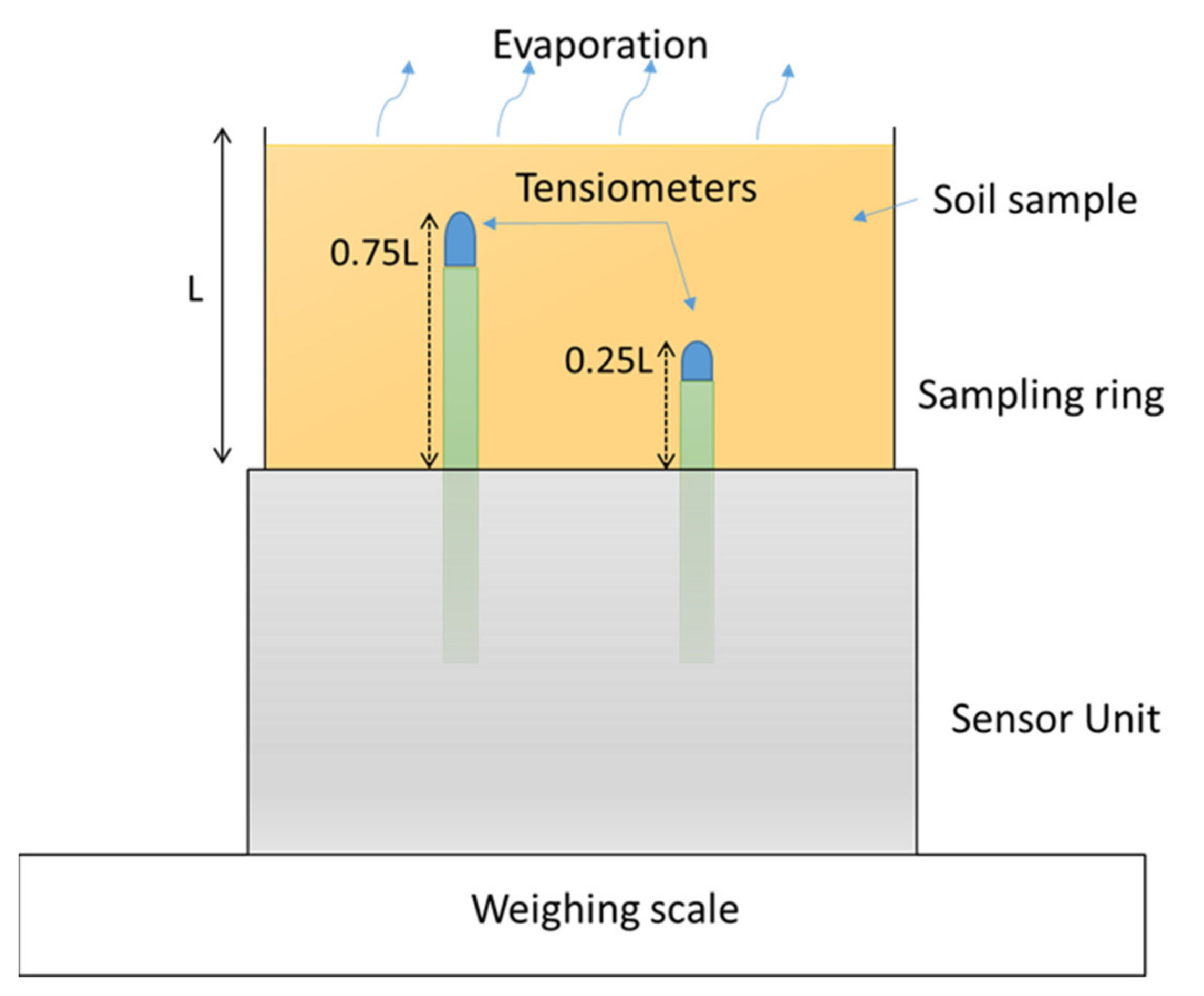
Schindler and Müller [20] published a soil hydraulic international dataset using the Evaporation method and HYPROP^TM (Hydraulic Property Analyzer, Meter Group Inc., USA) system. The HYPROP system (Figure 1) is an automated evaporation-based benchtop laboratory system that works based on the extended evaporation method [21,22]. The HYPROP has a relatively fast measurement cycle and provides high resolution reliable simultaneous measurements of soil water content and unsaturated hydraulic conductivity within a few days or weeks [23,24,25]. Haghverdi et al. [26] used an HYPROP measured Turkish soil data set to develop water retention PC_NN-PTFs and reported promising results. In a companion paper (Singh et al. [27]), we utilized the Schindler and Müller [20] dataset to develop water retention PC_NN-PTFs. However, no PC_NN-PTF has been developed to estimate the SHCC using high-resolution data measured via the evaporation method. Consequently, this study was carried out to (I) develop PC_NN-PTFs for SHCC estimations by utilizing the abovementioned international [20] and Turkish [26] data sets measured via the evaporation method, (II) determine the accuracy and reliability of the PC_NN-PTFs, and (III) assess the performance of the developed models across soil textures and different ranges of soil tension.

2. Materials and Methods

2.1. Soil Data Sets

In this study, two soil data sets were used to develop hydraulic conductivity PC_NN-PTFs and evaluate their accuracy and reliability. The measured hydraulic conductivity data and the soil textural classification of the samples for both data sets are shown in Figure 2. The primary data set, hereafter referred to as the international data set, was published by Schindler & Müller [20] and consisted of 173 soils collected from 71 sites from all over the world. This data set contains the measurements of water retention, unsaturated hydraulic conductivity, K(h), and several basic soil properties, including textural data, organic matter content (SOM), and dry bulk density (BD). The soil hydraulic properties were measured using the evaporation experiments or the extended evaporation method via the HYPROP method. A majority of the soil samples in the data set were collected from arable lands, yet few samples from other land use types such as urban land, grassland, forests, fallow lands and riverbanks were also present. After screening the international data set, a subset of samples (i.e., 150 soils with 6963 total K(h) data pairs) was selected to develop PC_NN-PTFs. The characteristics of the selected soils are shown in

Table 1. Characteristics of soils from international and Turkish data sets used in this study to develop and test pseudo continuous neural network pedotransfer functions (PC_NN-PTFs).

	International Data (150 Soil Samples with 6963 Data Pairs)			Turkish Data (79 Soil Samples with 1340 Data Pairs)
Attribute	Mean	Range	SD	Mean	Range	SD
Clay (%)	20.0	0.0–60.0	12.5	34.1	9.4–62.2	15.1
Silt (%)	56.4	0.2–86.8	17.1	30.7	5.2–57.6	8.7
Sand (%)	23.6	3.9–99.8	17.4	35.3	6.0–84.0	17.4
Bulk density (g cm−3)	1.3	0.6–1.7	0.2	1.0	0.7–1.3	0.1
Organic matter content (%)	3.1	0.0–12.0	2.5	1.2	0.0–3.1	0.6

SD: Standard deviation.

. The most dominant texture was silt loam; comprising 78 soil samples (52% of the data set), followed by loam; consisting of 18 soil samples (12% of the data set). Values of K(h) were log-transformed because hydraulic conductivity data are generally log-normally distributed [11]. The measured log(K(h)) values ranged from −6.64 to 0.98 (0 to 9.65 cm d⁻¹), with an average of −2.26 (0.073 cm d⁻¹). The pF (logarithmic transformation of soil tension in cm of water) values ranged from 0.22 to 4.21, with an average of 2.47.

The second data set (referred to as the Turkish data set herein) was mainly collected from areas surrounding Ankara, Turkey, and consisted of 79 repacked soil samples with 1340 K(h) data pairs that were measured via the HYPROP system [26]. In this dataset, the K_s data (pF 0) were measured using the falling head method with the KSAT instrument (Meter Group Inc., Pullman, WA, USA). The K(h) points were measured for each sample with pF ranging from 1.80 to 3.91, with an average of 2.51, and log(K) ranging from −4.75 to 3.27 (0 to 1862 cm d⁻¹), with an average of −1.6 (0.03 cm d⁻¹). Clay was the dominant texture (38 soil samples or 48.1% of the data set), followed by sandy loam (13 samples or 16.5% of the data set). Further details about the laboratory procedures used to develop this data set are available in Haghverdi et al. [21,28,29,30]. More information about HYPROP’s measurement principles is available in Schindler et al. [28].

A statistical analysis conducted in the companion manuscript [27] using Mahalanobis distance [29] revealed that these two data sets were independent and most Turkish samples fall outside the domain of applicability of the international dataset.

2.2. Unsaturated Hydraulic Conductivity Calculations

During HYPROP measurements, saturated soil samples (closed from the base) were placed on a balance. Two tensiometers were positioned such that the tensiometers’ tips were at depths of 0.25 L cm and 0.75 L cm, where L was the soil column height (which is typically 5 cm in laboratory evaporation experiments). The soil surface was open to the ambient atmosphere so that the soil water could evaporate. The medial pF value of the sample was calculated based on the average value of the two tensions measured by two tensiometers and corresponding water content was calculated based on the mass change of the soil sample.

The hydraulic conductivity was calculated using the water flow velocity (q_i[cm/d]) between time points t_i-1 and t_i through a horizontal plane that laid exactly in the middle of the two tension-tips:

$$q_i= \frac{1}{2} \frac{\left(\mathsf{\Delta }{V}_i/\mathsf{\Delta }{t}_i\right)}{A}$$

(1)

where, ΔV_i is the change in water volume in the whole sample (cm³), Δt_i is the time interval between two consecutive measurement points, and A the cross-sectional area (cm²) of the column.

The data points for the hydraulic conductivity function were calculated by inverting Darcy’s equation as:

$$K_i\left(h_i\right)=\frac{-q_i}{\{\left(\frac{\mathsf{\Delta }{h}_i}{\mathsf{\Delta }z}\right)-1\}}$$

(2)

where, h_i (cm) is the time- and space-averaged tension, Δh_i is the difference of tensions between the two tensiometer tips, and Δz (cm) is the distance between the tensiometer tips. The calculations assume that moisture tension and water content distribute linearly through the column and, therefore, the arithmetic mean of the tensions at two points was used. This simplified assumption was shown to provide accurate results because linearity errors in fluxes and tensions cancel each other out. [23]. The effect of hysteresis on water flow and transport is well understood [30]. However, since HYPROP measurements are taken during natural evaporation-based drying of soil samples, only drying hydraulic path was considered in this study.

2.3. PC_NN-PTFs Development

A three-layer feed-forward perceptron model was developed using MATLAB R2019a (Mathworks, 2019). The transfer functions were the “hyperbolic tangent sigmoid” and “linear” for the hidden and the output layers, respectively. The Levenberg–Marquardt algorithm [31] was used for training the models. The maximum epoch (one complete pass of the training data set through the learning process) was set to 1000 and the best weights were loaded automatically for testing.

Soil samples were randomly partitioned into 5 folds such that 80% of the data were used for the development of the PC_NN-PTF models and 20% for testing the models. The bootstrap technique was used on the development set to generate 100 replica datasets, each containing approximately 67% of the data. The rest of the development data (~33%) were used for cross-validation of the NN models. The training process was terminated when the root mean square error (RMSE) of the cross-validation subset began to increase or remain unchanged. To find the optimal topology of the neural network, the number of neurons of the hidden layer was iteratively changed from 1 to 14. This process was repeated five times leaving aside a different fold as the test set each time, such that all samples in the data set were used for testing the models. The outputs of the 100 PC_NN-PTFs with optimum topology were averaged to obtain the hydraulic conductivity estimations.

2.4. Modeling Scenarios

We evaluated the accuracy and reliability of the PC_NN-PTFs (developed using the international and the Turkish data sets) with four combination models of the input attributes, including textural constituents—sand, silt, and clay (SSC), BD, and SOM (

Table 2. Combinations of input attributes used in this study to develop PC_NN-PTFs.

Model	Input Attributes
1	SSC, BD, SOM, pF
2	SSC, pF
3	SSC, BD, pF
4	SSC, SOM, pF

SSC: sand, silt, and clay percentages (%), BD: bulk density (cm³ cm⁻³), SOM: soil organic matter content (%), pF: the logarithmic transformation of soil tension in cm of water.

). Model 1 constituted all the input attributes and the logarithmic transformation of soil suction (pF). Model 2 included SSC and pF. Model 3 included SSC, BD, and pF. Model 4 included SSC, SOM, and pF. The log(K (cm/d)) was the output parameter corresponding to the input pF value.

Four data partitioning scenarios, as shown in

Table 3. Different data partitioning scenarios used in the study to train, test, and validate PC_NN-PTFs.

Scenario	Data Sets
S1	Training: International, Test: International.
S2	Training: Turkish, Test: Turkish.
S3	Training: International, Test: Turkish.
S4	Training: International + Turkish, Test: Turkish.

, were considered when the international data set was used for training and testing (scenario 1), the Turkish data set was used for training and testing (scenario 2), the international data were used for training and the Turkish data for validation (scenario 3), and a combination of the two data sets was used for training and the Turkish dataset for testing (scenario 4). The accuracy of PTFs was assessed using a randomly selected subset of the development data set that was not used to derive the PTF. The reliability was evaluated based on the performance of PTFs on an independent data set beyond the statistical training limits and the geographical training area of the development dataset. For example, we estimated the log(K) of the Turkish soil samples to assess the reliability of the PC_NN-PTFs derived using the international data set. The results of the modeling scenarios were assessed to (i) quantify the improvements in international PC_NN-PTFs for a specific region after incorporating local samples into the training data set and (ii) determining whether the international PC_NN-PTFs trained using the integrated data works as accurately as the local PC_NN-PTFs.

2.5. Model Evaluation

The root mean square error (RMSE, Equation (1)), mean absolute error (MAE, Equation (2)), mean bias error (MBE, Equation (3)), and correlation coefficient (R, Equation (4)) were calculated for the test data to evaluate the performance of PC_NN-PTFs:

$$RMSE=\sqrt{\frac{1}{n}{\displaystyle \sum }_{i=1}^n{\left(E_i-M_i\right)}^2}$$

(3)

$$MAE=\frac{1}{n}{\displaystyle \sum }_{i=1}^n\left|E_i-M_i\right|$$

(4)

$$MBE=\frac{1}{n}{\displaystyle \sum }_{i=1}^n\left(E_i-M_i\right)$$

(5)

$$R=\frac{{{\displaystyle \sum }}_{i=1}^n\left(E_i-\overline{E})(M_i-\overline{M}\right)}{{{\displaystyle \sum }}_{i=1}^n{\left(E_i-\overline{E}\right)}^2{{\displaystyle \sum }}_{i=1}^n{\left(M_i-\overline{M}\right)}^2}$$

(6)

where, E and M are the estimated and measured log(K), respectively; $\overline{E}$ and $\overline{M}$ are the mean estimated and measured log(K), respectively; and n is the total number of measured water retention points for each model. In addition, the error statistics were calculated separately for dominant soil textures at the wet (pF ≤ 2), intermediate (2 < pF ≤ 3), and dry ranges (pF > 3) of the SHCC.

3. Results

3.1. Importance of the Input Predictors

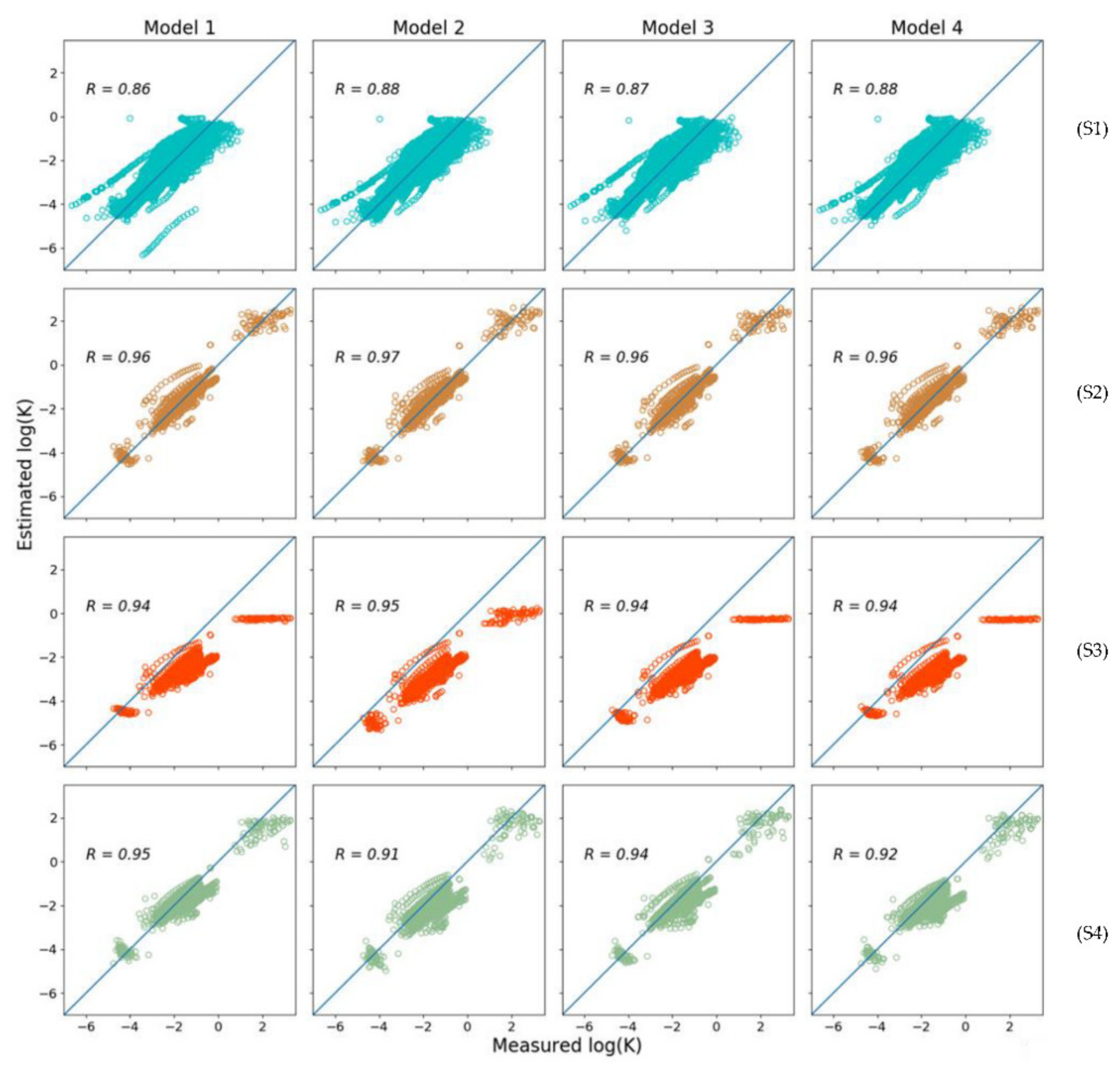
Figure 3 shows the scatterplots of measured versus estimated log(K) values for the PC_NN-PTFs developed in this study using different combinations of input predictors. All models showed acceptable performance, demonstrated by the well-scattered data around the 1:1 reference line except for the K_s estimations in scenario 3 (training: the international dataset, test: Turkish datasets).

Table 4. Performance of the PC_NN-PTFs estimating log-transformed soil hydraulic conductivity data (cm d⁻¹) across four modeling scenarios.

	Training and Test: I				Training and Test: T				Training: I.; Test: T				Training: I + T; Test: T
M	RMSE	MAE	MBE	R	RMSE	MAE	MBE	R	RMSE	MAE	MBE	R	RMSE	MAE	MBE	R
1	0.571	0.428	0.013	0.855	0.343	0.227	0.023	0.959	1.097	0.971	−0.959	0.935	0.429	0.312	−0.139	0.947
2	0.520	0.406	0.027	0.881	0.317	0.217	0.011	0.965	1.317	1.254	−1.249	0.954	0.613	0.456	−0.335	0.906
3	0.547	0.418	0.033	0.868	0.336	0.219	0.017	0.961	1.235	1.142	−1.133	0.942	0.453	0.308	−0.165	0.938
4	0.529	0.417	0.022	0.877	0.350	0.243	0.043	0.958	1.243	1.144	−1.132	0.943	0.554	0.400	−0.280	0.920

M: Model, RMSE: Root mean square error, MAE: mean absolute error, MBE: mean biased error, R: correlation coefficient. I: international data set, T: Turkish data set.

summarizes the performance statistics of the models for all the scenarios. For scenario 1 (training: International, test: International), Model 2 (inputs: SSC, pF) resulted in the best performance with an RMSE of 0.520 and MAE of 0.406, followed by Model 4 (SSC, SOM, pF) where RMSE was 0.529 and MAE was 0.417. The lowest performance was observed in model 1 where RMSE was 0.571 and MAE was 0.428. MBE varied from 0.013 to 0.033, demonstrating no substantial under or overestimation of log(K) for all models. The R values varied from 0.855 to 0.881, showing a high agreement between measured and estimated log(K) in all models.

For scenario 2 (training: Turkish dataset, test: Turkish dataset), Model 2 (inputs: SSC, pF) resulted in the best performance with RMSE of 0.317 and MAE of 0.217, followed by Model 3 (inputs: SSC, BD) where RMSE was 0.336 and MAE was 0.219. MBE varied from 0.011 for model 2 to 0.043 for model 4, demonstrating no considerable under or overestimation of log(K). The R values were high (between 0.958 and 0.965) and similar among all models.

For scenario 3 (training: the international data set, test: the Turkish data set), model 1 with RMSE of 1.097 and MAE of 0.971 performed the best. Model 2 with RMSE of 1.317 and MAE of 1.254 showed lower accuracy compared to the other models. The estimated log(K) values were highly correlated with the measured data (R: 0.935–0.954), yet all models showed an underestimation tendency (MBE ranging from −1.249 to −0.959). This is evident in Figure 3 as well, where data points are well scattered but located mainly below the 1:1 line.

For scenario 4 (training: combined international and Turkish data sets, test: the Turkish data set), the best performance was observed for Model 3 with RMSE of 0.453 and MAE of 0.308. Model 1 also had a similar performance. Slight underestimation of log(K) was observed with MBE ranging from −0.335 for model 2 to −0.139 for Model 1. Correlation between observed and estimated log(K) was high and similar among all models, with R values ranging from 0.906 to 0.947.

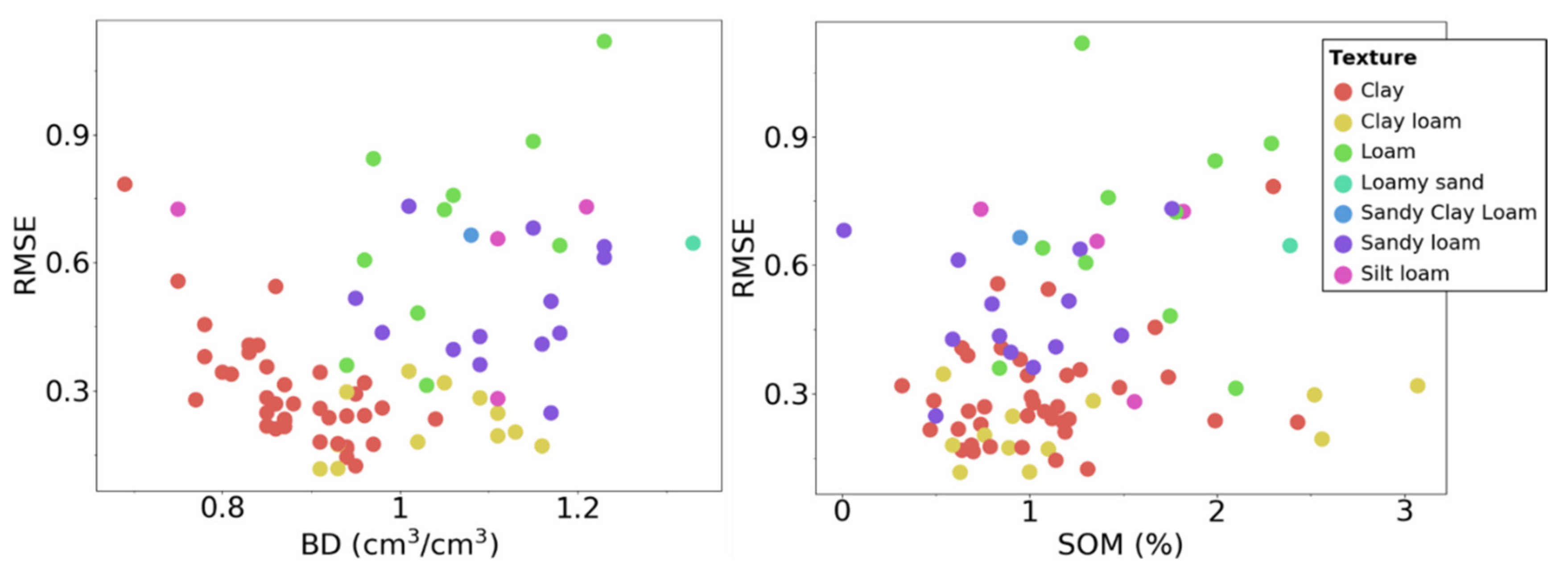
No distinct relationship was observed between BD and SOM with RMSE values except for the Turkish clay soils where RMSE declined as BD increased (Figure 4).

3.2. Performance across Soil Textures

The following analysis was only conducted using model 1 as the best performing PTF in the test phase.

Table 5. Performance of PC-PTFs on main textural classes of the international and Turkish data sets for estimating log(K).

Data Sets	Texture	RMSE	MAE	MBE	R
Training: I; Test: I	SiL	0.517	0.421	0.026	0.881
	L	0.612	0.485	−0.180	0.789
	SiCL	0.433	0.342	0.144	0.870
	CL	1.124	0.748	0.288	0.603
	SL	0.593	0.522	0.042	0.700
Training: T, Test: T	C	0.252	0.174	0.006	0.978
	SL	0.366	0.277	−0.096	0.966
	CL	0.206	0.146	0.018	0.982
	L	0.395	0.312	−0.048	0.926
Training: I, validation: T	C	0.986	0.863	−0.860	0.961
	SL	1.353	1.241	−1.223	0.96
	CL	0.964	0.894	−0.894	0.978
	L	1.444	1.377	−1.370	0.917
Training: I and T, Test: T	C	0.303	0.218	−0.013	0.972
	SL	0.535	0.446	−0.317	0.963
	CL	0.230	0.173	−0.094	0.985
	L	0.745	0.683	−0.614	0.915

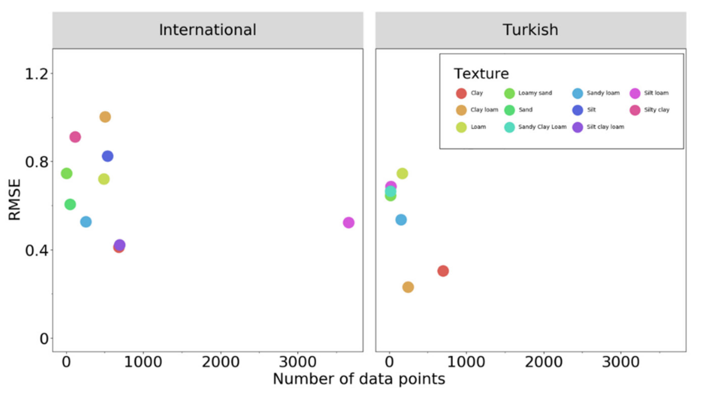
RMSE: Root mean square error, MAE: mean absolute error, MBE: mean biased error, R: correlation coefficient. I: international data set, T: Turkish data set. SiL: Silt Loam: L: Loam, SiCL: Silty Clay Loam, CL: Clay loam, SL: Sandy Loam, C: Clay.

shows the performance of the PC_NN-PTF models for the dominant soil textures, representing about 89% and 92% of the international and Turkish data sets, respectively. When the international data set was used as the training set (scenario 1), clay loam had higher RMSE and MAE values than other soil textures. RMSE values ranged from 0.517 to 1.124, MAE values ranged from 0.342 to 0.748, and MBE values ranged from 0.026 to 0.288 for all textures. Furthermore, the model showed a tendency to overestimate log(K) for all soil textures, except loam, where underestimation of log(K) was observed. The correlation coefficient (R) values varied between 0.603 in clay loam to 0.881 for silt loam.

When only Turkish data were used for training (scenario 2), RMSE and MAE values varied from 0.206 to 0.395 and 0.146 to 0.312, respectively. MBE values ranged from −0.096 for sandy loam to 0.018 for clay loam, and no substantial underestimation or overestimation of log(K) was observed. The agreement between the measured and estimated log(K) values was very high, indicated by high and similar R values (between 0.926 and 0.982) for all the models within each soil texture.

When the international data set was used for training and the Turkish data set for validation (scenario 3), RMSE and MAE values varied from 0.964 to 1.444 and 0.863 to 1.377, respectively. Underestimation of log(K) was observed for all the soil textures with MBE values ranging from −1.370 to −0.860. Loam had the highest error relative to other soil textures, while clay had the lowest. High and similar correlation coefficient values (between 0.917 and 0.978) were observed for all the models and soil textures.

When the Turkish data set was used as a test and a combination of international and Turkish data sets were used for the training (scenario 4), the RMSE and MAE values varied from 0.230 to 0.745 and 0.173 to 0.683, respectively. The loam and sandy loam had higher RMSE and MAE values, while the errors for clay loam and clay were similar to when just the Turkish data were used for training (scenario 2). The MBE values ranged from −0.614 to −0.013, showing slight underestimation of log (K) for most soil textures except clay and clay loam where underestimation was not substantial. The agreement between the estimated and observed log(K) was high, as depicted by the high R values (ranging from 0.915 to 0.985) for all the models.

3.3. Performance at the Wet, Intermediate and Dry Parts of the SHCC

Table 6. Performance of the PC_NN-PTFs (inputs: SSC, BD, OM, and pF) developed to estimate the log(K) at wet (pF ≤ 2) intermediate (2 < pF ≤ 3) and dry (pF > 3) parts of the SHCC.

	Training and Test: I			Training and Test: T			Training: I, Validation: T			Training: I and T, Test: T
	Wet	Mid	Dry	Wet	Mid	Dry	Wet	Mid	Dry	Wet	Mid	Dry
RMSE	0.548	0.570	0.603	0.588	0.317	0.375	2.285	1.002	0.466	0.757	0.400	0.396
MAE	0.420	0.440	0.381	0.471	0.206	0.298	2.158	0.936	0.342	0.602	0.291	0.322
MBE	−0.060	0.007	0.140	0.031	0.016	0.109	−2.158	−0.926	−0.292	−0.520	−0.134	0.154
R	0.509	0.640	0.522	0.809	0.860	0.831	0.768	0.785	0.860	0.805	0.791	0.818

RMSE: Root mean square error, MAE: mean absolute error, MBE: mean biased error, R: correlation coefficient. I: International data set, T: Turkish data set.

shows the performance of different PC_NN-PTFs over three moisture ranges of the SHCC for the four data partitioning scenarios evaluated in this study. When the international data set was used for the training and testing of the models (scenario 1), the RMSE of Model 1 varied from 0.548 in the wet range to 0.603 in the dry range. The MAE values varied from 0.420 in the wet range to 0.440 in the intermediate range of the SHCC. The MBE values varied between −0.060 in the wet range to 0.140 in the dry range. The R values ranged from 0.509 for the wet to 0.640 in the intermediate range.

When only Turkish data were used for the training and testing of the PC_NN-PTF models (scenario 2), the lowest error was observed in the intermediate range (RMSE = 0.317, MAE = 0.206, and MBE = 0.016) and the highest error belonged to the wet range (RMSE = 0.588, MAE = 0.471, and MBE = 0.031). The agreement between the observed and estimated log(K) was comparable among models with R ranging from a minimum of 0.809 in the wet range to a maximum of 0.860 in the intermediate range.

When the Turkish data were used as the validation data set (scenario 3), the PTFs showed their highest performance in the dry range (RMSE = 0.466 and MAE = 0.342) and their lowest performance in the wet range (RMSE = 2.285 and MAE = 2.158). Despite high R values (0.768–0.860), a tendency to underestimate log(K) was observed in all regions, as indicated by negative MBE ranging from −0.292 to −2.158.

When both international and Turkish data sets were used for the training of the models (scenario 4), the lowest error values were observed in the dry range (RMSE = 0.396 and MAE = 0.322) and the highest error in the wet range (RMSE = 0.757 and MAE = 0.602). RMSE values varied from 0.396 in the dry range to 0.757 in the wet range. Negative MBE values of −0.52 and −0.134 indicated a tendency to underestimate log(K) in the wet and intermediate ranges, respectively. The R values were high across all soil tension ranges.

4. Discussion

4.1. Accuracy and Reliability of the Developed PTFs

In our study, the best international hydraulic conductivity PC_NN-PTF showed the accuracy (same data set for development and test) and reliability (independent data sets for development and test) of RMSE = 0.520 and 1.097, respectively. The local PC_NN-PTF developed and tested using the Turkish dataset showed even higher performance, as expected, with an RMSE of 0.317. Parasuraman et al. (2006) stated that better performance in estimating K_s is observed when a NN model is trained even on a small set of relevant data rather than a larger general dataset. Our study emphasizes that a local data set, when available, should be included in the training of PC_NN-PTF for a more accurate estimation of the SHCC.

Schaap and Leij [6] reported RMSE values ranging from 1.12 to 1.76 for calibration subset and from 1.18 to 1.77 for an independent validation data set for their hydraulic conductivity PTFs, indicating lower accuracy and reliability than the PC_NN-PTF developed in this study. Børgesen et al. [7] reported a reasonable accuracy for their hydraulic conductivity PTFs with RMSE ranging from 0.598 to 1.196, yet most of the models showed underestimation. The above mentioned studies used the typical procedure to estimate the SHCC, which relies on estimated or measured K_s values and parametric SWRC PTFs using NN approach combined with bootstrap. Therefore, the PC_NN-PTFs approach developed and tested for the first time in this study could be used as an alternative high-performance approach to estimate the SHCC.

Large data sets being used to develop international PTFs typically consist of smaller data sets, employing different techniques to measure soil hydraulic properties. The commonly used devices have discrepancies in K_s measurements because of factors such as sample size, soil conditions, flow geometry and installation procedures [32]. The same is true for the various devices used for unsaturated hydraulic conductivity measurements such as the steady-state pressure membrane method, tension disc infiltrometer, hot-air methods, and the widely used multistep outflow method [33,34,35]. We recommend using HYPROP data sets for developing hydraulic conductivity PC_NN-PTFs. PC_NN-PTF takes advantage of the high resolution measured data provided by the HYPROP system to learn the shape of the SHCC directly from the actual measured data points, unlike the parametric PTFs where the relationships between the parameters and their predictors have to be known a priori. Furthermore, using only one method (evaporation experiment) for obtaining hydraulic conductivity data in the laboratory is expected to improve the performance of the PC_NN-PTFs by eliminating the variance related to employing multiple measurement techniques.

4.2. Importance of Input Variables

Studies have shown that the systematic variation in K_s is explained by properties like soil texture, porosity, SOM, and BD [36,37]. According to Zhang and Schaap [38], adding BD and SOM as input predictors improved the performance of PTFs in most studies estimating the K_s. Moosavi and Sepaskhah [12] observed that the combination of inputs SSC, BD, SOM (Model 1 in this study) and SSC (Model 2 in this study) produced the best accuracy in estimating unsaturated hydraulic conductivity. In our study, considering SOM and BD as extra input attributes in addition to soil texture did not improve the accuracy of the international and local PTFs (scenarios 1 and 2). However, adding BD and SOM as input attributes noticeably enhanced the performance of the PC_NN-PTF in scenarios 3 and 4. This result differs from our observation in the companion paper (Singh et al. [27]), where adding SOM as an extra input did not improve the performance of the water retention PC_NN-PTFs.

Except for scenario 1, BD was a more effective additional attribute than SOM in all modeling scenarios. Improvements in the estimation of log(K) were observed in other studies too when BD was included as an additional PTF input predictor [6,39]. The BD, however, only provides limited information about soil structure as different preferential flow pathways may result in substantially different soil hydraulic conductivities [40]. Hao et al. [41] reported that K_s is influenced primarily by porosity and macro water-stable aggregates, which are not among typical PTF inputs. Further studies are needed to determine the impact of considering additional soil structural input parameters on the performance of hydraulic conductivity PC_NN-PTF.

4.3. Performance across Textural Classes and Tension Ranges

The PC_NN-PTFs showed better performance for fine-textured (Clay and Clay Loam) than more coarse-textured (Loam and Sandy Loam) Turkish soils (scenarios 2, 3, and 4), which is attributed to a relatively higher number of fine-textured Turkish soil samples. We observed an overall improvement in the performance of PTFs with the increasing number of data points per soil textural class (Figure 5). These results concur with the results we reported in the companion paper (Singh et al. [27]), where high performance was observed for the dominant soil textures for the SWRC estimations. Since PC_NN-PTFs are machine learning-based models, their performance is expected to improve as more data become available for training.

The performance of PC_NN-PTFs was consistent across tension ranges when developed and tested using the international data set, which concurs with the results observed in the companion paper for soil water retention estimations [27]. Moosavi and Sepaskhah [12] reported a relatively lower accuracy of the NN-based PTFs to estimate hydraulic conductivity at the saturated and/or near-saturated tensions. We observed a somewhat higher error in the wet tension region (pF ≤ 2) for the Turkish data set, primarily when PC_NN-PTFs were developed using the international data set. In our companion paper, however, the performance of water retention PC_NN-PTFs was similar in three tension regions. The relatively higher error in the wet range in this study was because the Turkish data set only contained K_s data in the wet part (measured via the KSAT instrument), while K_s measurements were not available for the international data set.

5. Conclusions

We developed and evaluated PC_NN-PTFs to estimate the SHCC measured using the evaporation experiments, mainly via the HYPROP system. The PC_NN-PTF approach showed promising performance for continuous hydraulic conductivity estimation over a wide range of soil tensions. The HYPROP system offers the advantage of producing high-resolution soil hydraulic conductivity data over a wide range of soil tensions (pF = 1.5 to 3.5), which is critical for developing robust PC_NN-PTF models since this approach learns the shape of the SHCC directly from measured data. The KSAT instrument can be employed to measure the saturated hydraulic conductivity (K_s) that can be used along with HYPROP data. The water retention PC_NN-PTFs developed and validated in the first part of this study (Singh et al. [27]) also performed very well. Consequently, we recommend the PC_NN-PTF approach to derive the next generation of water retention and hydraulic conductivity models using high-resolution data measured via the HYPROP system.

References

1. Bouma, J. Using Soil Survey Data for Quantitative Land Evaluation. In Advances in Soil Science; Stewart, B., Ed.; Springer: New York, NY, USA, 1989; Volume 9, ISBN 978-1-4612-3532-3. [Google Scholar]
2. Vereecken, H.; Schnepf, A.; Hopmans, J.W.; Javaux, M.; Or, D.; Roose, T.; Vanderborght, J.; Young, M.H.; Amelung, W.; Aitkenhead, M.; et al. Modeling Soil Processes: Review, Key Challenges, and New Perspectives. Vadose Zo. J. 2016, 15, 1–57. [Google Scholar] [CrossRef] [Green Version]
3. Assouline, S.; Or, D. Conceptual and Parametric Representation of Soil Hydraulic Properties: A Review. Vadose Zo. J. 2013, 12. [Google Scholar] [CrossRef]
4. Van Genuchten, M.T. A Closed-form Equation for Predicting the Hydraulic Conductivity of Unsaturated Soils1. Soil Sci. Soc. Am. J. 1980, 44, 892. [Google Scholar] [CrossRef] [Green Version]
5. Mualem, Y. A new model for predicting the hydraulic conductivity of unsaturated porous media. Water Resour. Res. 1976, 12, 513–522. [Google Scholar] [CrossRef] [Green Version]
6. Schaap, M.G.; Leij, F.J. Using neural networks to predict soil water retention and soil hydraulic conductivity. Soil Tillage Res. 1998, 47, 37–42. [Google Scholar] [CrossRef]
7. Børgesen, C.D.; Iversen, B.V.; Jacobsen, O.H.; Schaap, M.G. Pedotransfer functions estimating soil hydraulic properties using different soil parameters. Hydrol. Process. 2008, 22, 1630–1639. [Google Scholar] [CrossRef]
8. Parasuraman, K.; Elshorbagy, A.; Si, B.C. Estimating Saturated Hydraulic Conductivity In Spatially Variable Fields Using Neural Network Ensembles. Soil Sci. Soc. Am. J. 2006, 70, 1851–1859. [Google Scholar] [CrossRef] [Green Version]
9. Schaap, M.G.; Leij, F.J.; van Genuchten, M.T. Neural Network Analysis for Hierarchical Prediction of Soil Hydraulic Properties. Soil Sci. Soc. Am. J. 1998, 62, 847. [Google Scholar] [CrossRef]
10. Weynants, M.; Vereecken, H.; Javaux, M. Revisiting Vereecken Pedotransfer Functions: Introducing a Closed-Form Hydraulic Model. Vadose Zo. J. 2009, 8, 86–95. [Google Scholar] [CrossRef] [Green Version]
11. Schaap, M.G.; Leij, F.J. Improved Prediction of Unsaturated Hydraulic Conductivity with the Mualem-van Genuchten Model. Soil Sci. Soc. Am. J. 2000, 64, 843–851. [Google Scholar] [CrossRef] [Green Version]
12. Moosavi, A.A.; Sepaskhah, A. Artificial neural networks for predicting unsaturated soil hydraulic characteristics at different applied tensions. Arch. Agron. Soil Sci. 2012, 58, 125–153. [Google Scholar] [CrossRef]
13. Wagner, B.; Tarnawski, V.R.; Hennings, V.; Muller, U. Evaluation of pedo-transfer functions for unsaturated soil hydraulic conductivity using an independent data set. Geoderma 2001, 102, 275–297. [Google Scholar] [CrossRef]
14. Niemann, W.L.; Rovey, C.W. A systematic field-based testing program of hydraulic conductivity and dispersivity over a range in scale. Hydrogeol. J. 2009, 17, 307–320. [Google Scholar] [CrossRef]
15. Bormann, H.; Klaassen, K. Seasonal and land use dependent variability of soil hydraulic and soil hydrological properties of two Northern German soils. Geoderma 2008, 145, 295–302. [Google Scholar] [CrossRef]
16. Baroni, G.; Facchi, A.; Gandolfi, C.; Ortuani, B.; Horeschi, D.; Van Dam, J.C. Uncertainty in the determination of soil hydraulic parameters and its influence on the performance of two hydrological models of different complexity. Hydrol. Earth Syst. Sci. 2010, 14, 251–270. [Google Scholar] [CrossRef] [Green Version]
17. Fodor, N.; Sándor, R.; Orfanus, T.; Lichner, L.; Rajkai, K. Evaluation method dependency of measured saturated hydraulic conductivity. Geoderma 2011, 165, 60–68. [Google Scholar] [CrossRef]
18. Haghverdi, A.; Cornelis, W.M.; Ghahraman, B. A pseudo-continuous neural network approach for developing water retention pedotransfer functions with limited data. J. Hydrol. 2012, 442–443, 46–54. [Google Scholar] [CrossRef]
19. Haghverdi, A.; Öztürk, H.S.; Cornelis, W.M. Revisiting the pseudo continuous pedotransfer function concept: Impact of data quality and data mining method. Geoderma 2014, 226–227, 31–38. [Google Scholar] [CrossRef]
20. Schindler, U.; Müller, L. Soil hydraulic functions of international soils measured with the Extended Evaporation Method (EEM) and the HYPROP device. Open Data J. Agric. Res. 2017, 3, 10–16. [Google Scholar] [CrossRef] [Green Version]
21. Schindler, U.; Durner, W.; von Unold, G.; Mueller, L.; Wieland, R. The evaporation method: Extending the measurement range of soil hydraulic properties using the air-entry pressure of the ceramic cup. J. Plant Nutr. Soil Sci. 2010, 173, 563–572. [Google Scholar] [CrossRef]
22. Schindler, U.; Durner, W.; von Unold, G.; Müller, L. Evaporation Method for Measuring Unsaturated Hydraulic Properties of Soils: Extending the Measurement Range. Soil Sci. Soc. Am. J. 2010, 74, 1071. [Google Scholar] [CrossRef]
23. Peters, A.; Iden, S.C.; Durner, W. Revisiting the simplified evaporation method: Identification of hydraulic functions considering vapor, film and corner flow. J. Hydrol. 2015, 527, 531–542. [Google Scholar] [CrossRef]
24. Peters, A.; Durner, W. Simplified evaporation method for determining soil hydraulic properties. J. Hydrol. 2008, 356, 147–162. [Google Scholar] [CrossRef]
25. Bezerra-Coelho, C.R.; Zhuang, L.; Barbosa, M.C.; Soto, M.A.; Van Genuchten, M.T. Further tests of the HYPROP evaporation method for estimating the unsaturated soil hydraulic properties. J. Hydrol. Hydromech. 2018, 66, 161–169. [Google Scholar] [CrossRef] [Green Version]
26. Haghverdi, A.; Öztürk, H.S.; Durner, W. Measurement and estimation of the soil water retention curve using the evaporation method and the pseudo continuous pedotransfer function. J. Hydrol. 2018, 563, 251–259. [Google Scholar] [CrossRef]
27. Singh, A.; Haghverdi, A.; Öztürk, H.S.; Durner, W. Developing Pseudo Continuous Pedotransfer Functions for International Soils Measured with the Evaporation Method and the HYPROP System: I. The Soil Water Retention Curve. Water 2020, 12, 3425. [Google Scholar] [CrossRef]
28. Schindler, U.; Mueller, L.; von Unold, G.; Durner, W.; Fank, J. Emerging Measurement Methods for Soil Hydrological Studies. In Novel Methods for Monitoring and Managing Land and Water Resources in Siberia; Springer: Cham, Switzerland, 2016; pp. 345–363. ISBN 978-3-319-24409-9. [Google Scholar]
29. Tranter, G.; McBratney, A.B.; Minasny, B. Using distance metrics to determine the appropriate domain of pedotransfer function predictions. Geoderma 2009, 149, 421–425. [Google Scholar] [CrossRef]
30. Yang, H.; Khoshghalb, A.; Russell, A.R. Fractal-based estimation of hydraulic conductivity from soil-water characteristic curves considering hysteresis. Geotech. Lett. 2014, 4, 1–10. [Google Scholar] [CrossRef]
31. Marquardt, D.W. An Algorithm for Leat-Squares Estimation of Nnonlinear Parameters. J. Soc. Indust. Appl. Math. 1963, 11, 431–441. [Google Scholar] [CrossRef]
32. Morbidelli, R.; Saltalippi, C.; Cifrodelli, M. In situ measurements of soil saturated hydraulic conductivity: Assessment of reliability through rainfall—runoff experiments. Hydrol. Process. 2017, 3084–3094. [Google Scholar] [CrossRef]
33. Stolte, J.; Freijer, J.I.; Bouten, W.; Dirksen, C.; Halbertsma, J.M.; Van Dam, J.C.; Van den Berg, J.A.; Veerman, G.J.; Wösten, J.H.M. Comparison of Six Methods To Determine Unsaturated Soil Hydraulic Conductivity. Soil Sci. Soc. Am. J. 1994, 58, 1596–1603. [Google Scholar] [CrossRef]
34. Benson, C.H.; Gribb, M.M. Measuring unsaturated hydraulic conductivity in the laboratory and field. Geotech. Spec. Publ. 1997, 113–168. [Google Scholar]
35. Durner, W.; Lipsius, K. Determining Soil Hydraulic Properties. In Encyclopedia of Hydrological Sciences; Anderson, M.G., Mcdonnell, J., Eds.; John Wiley & Sons, Ltd.: Chichester, UK, 2005; Volume 2, pp. 1121–1144. [Google Scholar]
36. Cosby, B.J.; Hornberger, G.M.; Clapp, R.B.; Ginn, T.R. A Statistical Exploration of the Relationships of Soil Moisture Characteristics to the Physical Properties of Soils. Water Resour. Res. 1984, 20, 682–690. [Google Scholar] [CrossRef] [Green Version]
37. Wösten, J.H.M.; Lilly, A.; Nemes, A.; Le Bas, C. Development and use of a database of hydraulic properties of European soils. Geoderma 1999, 90, 169–185. [Google Scholar] [CrossRef]
38. Zhang, Y.; Schaap, M.G. Estimation of saturated hydraulic conductivity with pedotransfer functions: A review. J. Hydrol. 2019, 575, 1011–1030. [Google Scholar] [CrossRef]
39. Minasny, B.; Hopmans, J.W.; Harter, T.; Eching, S.O.; Tuli, A.; Denton, M.A. Neural Networks Prediction of Soil Hydraulic Functions for Alluvial Soils Using Multistep Outflow Data. Soil Sci. Soc. Am. J. 2004, 68, 417–429. [Google Scholar] [CrossRef]
40. Romero-Ruiz, A.; Linde, N.; Keller, T.; Or, D. A Review of Geophysical Methods for Soil Structure Characterization. Rev. Geophys. 2018, 56, 672–697. [Google Scholar] [CrossRef] [Green Version]
41. Hao, M.; Zhang, J.; Meng, M.; Chen, H.Y.H.; Guo, X.; Liu, S.; Ye, L. Impacts of changes in vegetation on saturated hydraulic conductivity of soil in subtropical forests. Sci. Rep. 2019, 9, 1–9. [Google Scholar] [CrossRef] [Green Version]
Figure 1. Experimental setup of the extended evaporation experiment using HYPROP system.
Water 13 00878 g001
Figure 2. The soil hydraulic conductivity and tension pairs (a), and soil textural distribution for the datasets (b). Dark orange circles depict the international data set [20] and blue circles represent the Turkish dataset [21,28,29,30]. pF is the logarithmic transformation of soil tension in cm of water and K is the unsaturated hydraulic conductivity.
Water 13 00878 g002
Figure 3. Scatterplots of measured versus estimated log(K) using PCNN-PTFs. S1: training and test: the international dataset, S2: Training and test: Turkish dataset, S3: training: the international dataset, test: Turkish dataset, S4: training: international + Turkish dataset, test: Turkish dataset. Model 1 inputs: sand, silt and clay percentages (SSC), bulk density (BD), and soil organic matter content (SOM); Model 2 inputs: SSC; Model 3 inputs: SSC, BD; Model 4 inputs: SSC and SOM.
Water 13 00878 g003
Figure 4. The root of mean squared error (RMSE) as a function of bulk density (BD) and organic matter content (SOM) for the PCNNPTF Model 1 with SSC, BD, SOM as inputs. The model was developed using combined international and Turkish data sets and tested using the Turkish data set (scenario 4). The error was calculated for each soil sample separately.
Water 13 00878 g004
Figure 5. The root of mean squared error (RMSE) as a function of the number of measured hydraulic conductivity data pairs for each textural class for the PCNN-PTF Model 1 with SSC, BD, SOM as inputs. The model was developed using combined international and Turkish data sets.
Water 13 00878 g005