Risk Assessment of Coastal Flooding under Different Inundation Situations in Southwest of Taiwan (Tainan City)

Abstract

The Pacific island countries are particularly vulnerable to the effects of global warming including more frequent and intense natural disasters. Seawater inundation, one of the most serious disasters, could damage human property and life. Regional sea level rise, highest astronomic tide, vertical land motions, and extreme sea level could result in episodic, recurrent, or permanent coastal inundation. Therefore, assessing potential flooding areas is a critical task for coastal management plans. In this study, a simulation of the static flooding situation in the southwest coast of Taiwan (Tainan city) at the end of this century was conducted by using a combination of the Taiwan Digital Elevation Model (DEM), regional sea level changes reconstructed by tide gauge and altimetry data, vertical land deformation derived from leveling and GPS data, and ocean tide models. In addition, the extreme sea level situation, which typically results from high water on a spring tide and a storm surge, was also evaluated by the joint probability method using tide gauge records. To analyze the possible static flood risk and avoid overestimation of inundation areas, a region-based image segmentation method was employed in the estimated future topographic data to generate the flood risk map. In addition, an extreme sea level situation, which typically results from high water on a spring tide and a storm surge, was also evaluated by the joint probability method using tide gauge records. Results showed that the range of inundation depth around the Tainan area is 0–8 m with a mean value of 4 m. In addition, most of the inundation areas are agricultural land use (60% of total inundation area of Tainan), and two important international wetlands, 88.5% of Zengwun Estuary Wetlands and 99.5% of Sihcao Wetlands (the important Black-faced Spoonbills Refuge) will disappear under the combined situation. The risk assessment of flooding areas is potentially useful for coastal ocean and land management to develop appropriate adaptation policies for preventing disasters resulting from global climate change.

1. Introduction

Sea level rise (SLR), one of the most severe disasters induced by global warming, could damage human property and life, especially for the inundation in low-lying coastal areas. The increase in mean sea level (MSL) may pose a higher risk of flooding in coastal zones, the intrusion of seawater, loss of wetlands, and inundation of low-lying areas [1,2,3].

Many of the coastal areas are densely populated and growing rapidly, including lots of metropolises in the world. While low elevation coastal zones below 10 m sea level only cover 2% of the global land area, they accommodate 10% of the world’s population and 13% of the world’s urban inhabitants [4,5]. The Pacific island countries are particularly vulnerable to the effects of global warming such as more frequent and intense natural disasters [6,7]. As observed by satellite altimetry, sea level has risen three times faster in the western Pacific Ocean than the global average since 1993, which mainly resulted from the non-uniform water volume changes due to the ocean temperature and salinity variations [8,9]. In addition, non-climatic factors of SLR such as geological processes and vertical land motions (VLM) usually amplify the relative SLR. Moreover, human-induced activities, including groundwater extraction or reduced sediment supply to river deltas caused by dam building, increase the vulnerability of the susceptible coastal zone and most low-lying river deltas in Asia [10,11]. Tides also affect sea level and cause severe damages when coinciding with storm surges. Tides are usually the largest sources of short-term sea level fluctuations [12].

Taiwan is a densely populated island country where most of the people live in plain and western lowlands with very small topographic gradient [13]. Compared to the other western Pacific countries, Taiwan is more vulnerable to global SLR, with consequently higher socio-economic impacts on human property and life. Both tide gauges and satellite altimetry data show the larger SLR trend in Taiwan than the global trend in 1961–2003 [6,7,8,9,10,11,12,13]. In addition, significant subsidence rates (3–31 mm/year) were observed by the Global Positioning System (GPS) and altimeter–tide gauge in the southwestern plains of Taiwan [14,15]. The amplitude of ocean tides in the west coast of Taiwan is larger than that in the east coast of Taiwan [16]. Taiwan is located in the path of the subtropical cyclone, typhoon. Taiwan is struck by typhoon disasters almost every summer, and the abundant rainfall brought by typhoons causes severe flooding [7].

While several coastal inundation analysis has been conducted [17,18], most studies have mainly focused on storm surge and rainfall contribution.

Torres et al. [19] analyzed the effects of storm surge and inland rainfall using a flow model and generated floodplain maps under hurricane situations. Passeri et al. [20] reported that tidal amplitudes within the bays increased by 67% under the highest SLR situation, while the ratio of the maximum flood to maximum ebb velocity decreased in the future situations by 26% and 39%. Meanwhile, Bilskie et al. [21] showed that the storm surge response to SLR is dynamic and sensitive to changes in the landscape, Doong et al. [22] developed a new generation of flood inundation maps at the city scale to demonstrate the effectiveness of such maps in the case of the coastal city of Tainan, Taiwan. Their study demonstrated that land elevation, tidal phase, and storm surge are the three dominant factors that influence flooding in Tainan.

Even though flood risk has been studied for a long time with the development of numerous approaches, several aspects have not yet been completely investigated such as the influence of the combined effect of contribution factors for long-term inundation prediction, considering the co-existence of SLR and VLM, which requires further analyses.

To analyze the possible static flood risk, the region growing algorithm method has been developed by imaging scientists [23,24]. Region growing, also called the flood-fill algorithm, is a region-based image segmentation algorithm to partition the image into regions that represent the same attribute by spatial continuity used in pixel-based image-segmentation on the selected initial seed point [25]. This image segmentation method has been widely applied to extract the water boundary from satellite and aerial images when generating the flood risk map to avoid overestimation [24].

Region growing combined with a Digital Elevation Model (DEM) can be used to assess the flood inundation extent. The region growing algorithm is a useful tool for estimating the long-term flooding, which depends primarily on elevation rather than short-term flooding attributed to the duration of flooding and surface roughness coefficients. This algorithm has been successfully applied to assess the inundation area of the static flood in other studies. Bins et al. [23] used the region growing algorithm to detect the land-use changes associated with water resources from the true color satellite image. Matgen et al. [26] employed the radiometric region growing, combining threshold to extract the flood extent from a Synthetic-Aperture Radar (SAR) image. In another study by Poulter and Halpin [27], a light detection and ranging (LiDAR) DEM was used to estimate the effects of SLR at North Carolina, USA. The modified DEM of future land subsidence and the prediction of flood water level was studied by Ward et al. [10] to estimate the future coastal flood hazard. Sea level was assumed constant in the above studies, so the model operated in a relatively simple way of determining the flooded area by subtracting the SLR constant from the elevation of DEM cell and performing the algorithm from an arbitrarily given seed point at open sea.

In addition to studying static flood inundation in the near future, assessment of the probability of extreme sea levels is necessary for modern coastal infrastructure designing. To estimate the extreme sea level and flood risk, several methods were developed for extra-tropical regions, where the extreme sea levels usually result from a combination of astronomical high tides and extreme weather effects [28]. One of the reliable probabilities of extreme levels is the joint tide-surge probability method (JPM), which significantly improves the extreme sea level analysis by splitting the measured sea level signal into tidal and surge components and performing statistical analysis for each component [29]. This approach has been successfully applied to the deep-water coastal area. However, in the shallow coastal regions, the factors contributing to sea level, such as tides and surges, cannot be treated as independent variables because of the interaction between surges and tides [30]. Therefore, Liu et al. [31] proposed the Direct Joint Probability Method (DJPM) to solve this problem, which requires a few assumptions regarding the amount and nature of the data and enables application to cases where dependent factors contributed to sea level fluctuation. DJPM provides a more statistically sound approach with a higher level of confidence.

Thus, the objective of this study is to assess the total coastal flooding area in the southwest coast of Taiwan during this century considering the regional sea level data derived from tide gauges and satellite altimeters, the crustal deformation from leveling and GPS, and the highest astronomical tide (HAT) from the regional tide model. In addition, the extreme sea level is evaluated by performing the DJPM on tide gauge records. Then, the probability of flooding risk around the coastal area is assessed using the recurrence level obtained from the DJPM. To avoid overestimation of the inundation zone, we develop a modification of the region-based image segmentation algorithm. Analysis of the coastal flooding trend of Taiwan and the risk assessment of these areas is potentially useful for the nearshore ocean and land management plan, and to develop appropriate adaptation policies for preventing disasters resulting from global climate change.

2. Study Area and Datasets

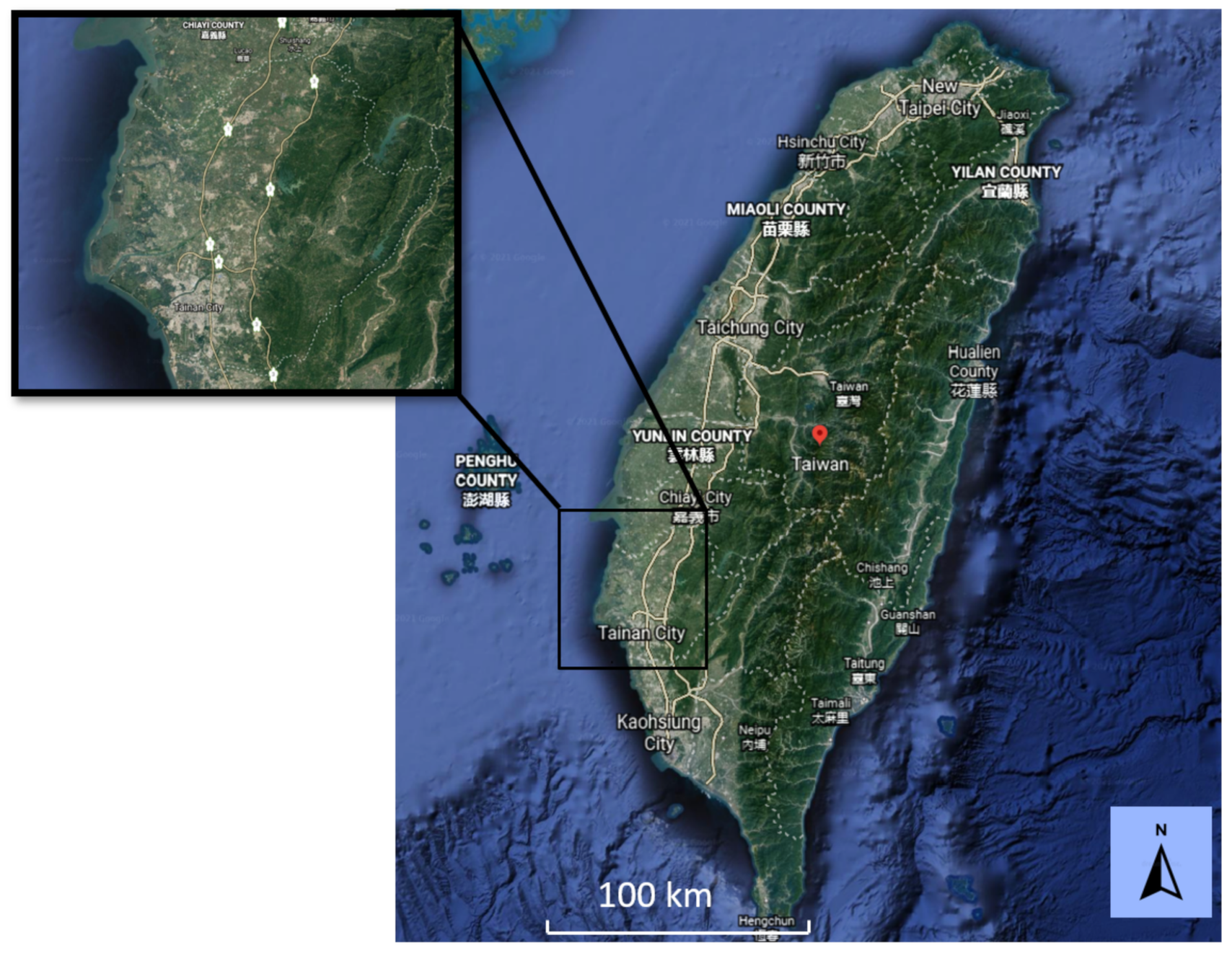
2.1. Taiwan, Tainan City

Taiwan is a densely populated island country lying about 180 km off the southeast of mainland China, which is located across the Taiwan Strait, with an area of 36,000 km². The topography of Taiwan is classified into two parts: the flat to gently rolling plains in the west, where 90% of the population lives, and the mostly rugged forest-covered mountains in the eastern two-thirds [32].

Therefore, the western floodplain in Taiwan is very vulnerable to SLR and extreme flood events from the perspective of population exposure [33]. In addition, anthropogenic land subsidence caused by excessive groundwater utilization at the western coastal plain cannot be neglected. According to the Government Report on Water Resources, more and more farmers in the southwestern coastal areas of Yunlin, Chiayi, and Tainan have expanded their business into aquaculture because of the profits and economical matter. Aquaculturists have dug many unregistered wells and pumped excessive amounts of groundwater, taking advantage of a cheap source of water with stable temperature. Moreover, land subsidence increases the vulnerability of inundation of the low-lying area, saltwater intrusion, and soil salinization, which results in the groundwater contamination and the loss of coastal wetlands [13].

Tainan city is located in southwestern Taiwan, which is a special municipality facing the Formosan Strait or Taiwan Strait in the west and south. Tainan is the oldest city on the island of Taiwan. Once reliant on traditional manufacturing industries, the region became a major high-tech industrial hub after the establishment of the Southern Taiwan Science Park in 1995. Agriculture is important to the city, especially the river north region. While fisheries and fish farming signify the coastal districts, and rice and fruit farms shaped the landscape of the inland agriculture region (Figure 1) [34].

Several important wetlands in Taiwan located near the southwest coast are listed in

Table 1. The list of important Taiwan coastal wetlands. ¹

Name	Location	Importance Level	Area (ha)
Zengwun Estuary Wetland	Tainan City	International importance	3218
Sihcao Wetland	Tainan City	International importance	547
Beimen Wetland	Tainan City	National importance	2447
Cigu Salt Pan Wetland	Tainan City	National importance	2997
Yanshuei Estuary Wetland	Tainan City	National importance	635
Bajhang Estuary Wetland	Chiayi County and Tainan City	National importance	634

¹ Vertical land motions.

. Taiwan has two wetlands of international importance according to Asian Wetland’s report from the International Union for Conservation of Nature (IUCN), including Zengwun Estuary Wetland and Sihcao Wetland, both of which are located in Tainan City (Figure 2). The Zengwun Estuary Wetland, situated at the mouth of the Zengwun River, is a bio-diversified habitat that attracts hundreds of Black-faced Spoonbills. The Sihcao Wetland is located in the intersection area where the Zengwun River, Luermen River, Yanshuei River, and Chianan Big Ditch meet, southwest of Provincial Highway 17. The wetland has more than 300 Black-faced Spoonbills visiting during winter, and around one hundred pairs of Black-winged Stilts breeds there. In addition, Sihcao meets the standards and guidelines of an important bird area (IBA). Furthermore, Sihcao has mangroves at the intersection area of seawater and land. It is considered as one of the most important and best-preserved habitats for mangrove growth, with the highest biodiversity along the Taiwan coastline.

2.2. Datasets

2.2.1. Digital Elevation Model

The Digital Elevation Model (DEM) is a 3D representation of the ground’s surface in a regular grid scale. With the intention of separating the simplest form of terrain relief modeling from more complex forms of digital surface representation, the term DEM was introduced in the 1970s. DEMs are a primary input to any modeling or process quantification that includes the topography of the earth, and they are used in many development areas [36]. The Taiwan DEM produced by the Satellite Survey Center, Department of Land Administration, Ministry of the Interior is applied in this study. The DEM in 5 m spatial resolution was generated in 2004 by aerial photography on 1:20,000 scale from the Aerial Survey Office, Forestry Bureau, Taiwan. The horizontal datum of DEM refers to Taiwan Datum 97 2-degree Transverse Mercator (TWD97 TM2) Projection System, and the vertical datum of DEM is related to Taiwan Vertical Datum 2001 (TWVD2001) [36].

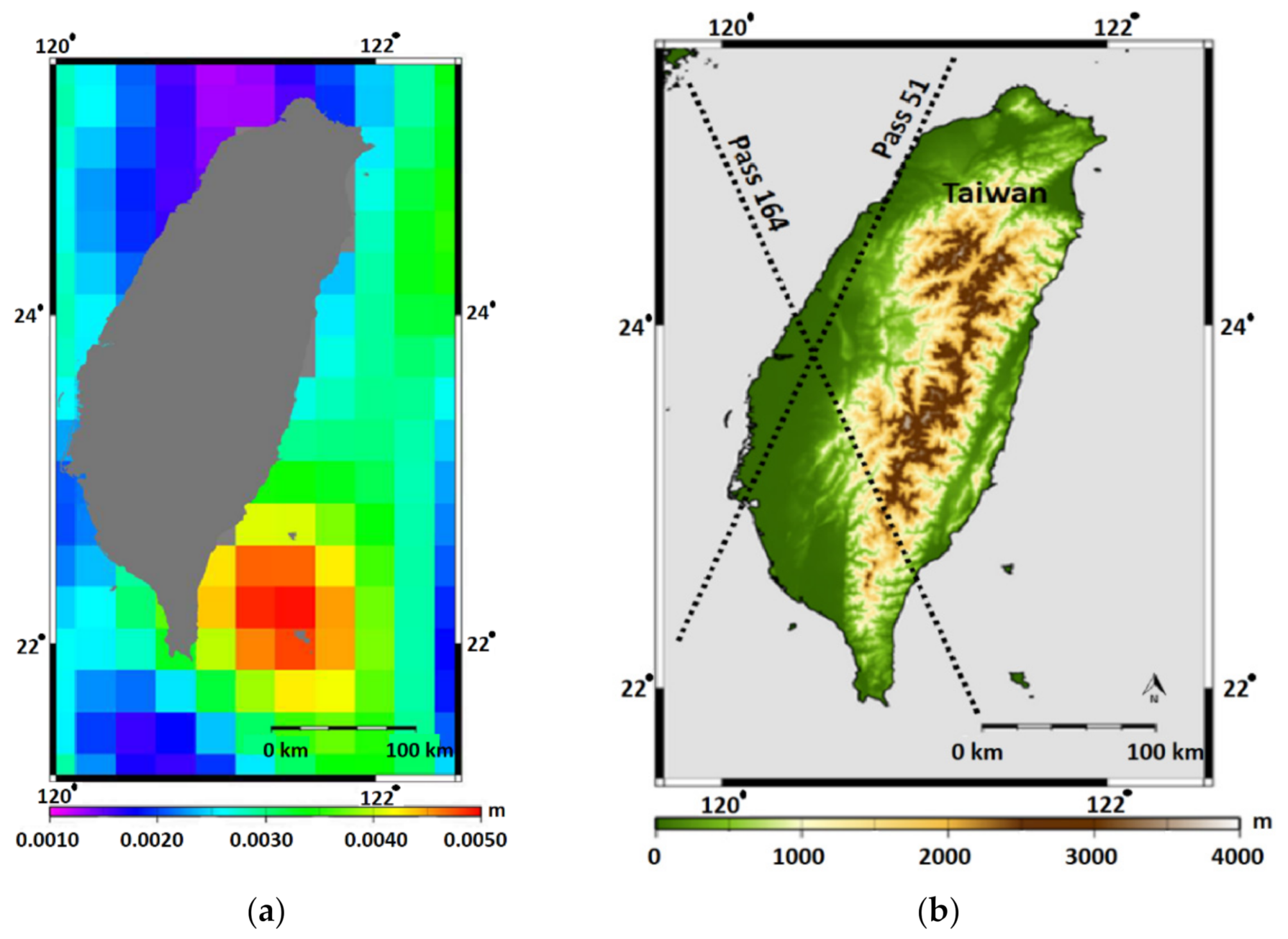
2.2.2. Satellite Altimetry

In this study, the global climatological monthly ¼° × ¼°gridded mean sea level anomalies from Archiving, Validation, and Interpretation of Satellite Oceanographic (AVISO) is applied (Figure 3) [37]. The data are underlying the delayed time and all-sat merged process. The time span covers from January 1993 to December 2012. The altimeter grid product has been processed with all standard corrections, including orbit, instrument, geophysical, and medium corrections. To assess the impact of SLR on the southwestern coastal areas of Taiwan, we use the six-parameter regression analysis method to estimate the gridded sea level trend around Taiwan, which is expressed as [38]:

$$SLA\left(t\right)=a+bt+c\sin 2\pi t+c\cos 2\pi t+e\sin 4\pi t+f\cos 4\pi t$$

(1)

where SLA is the monthly altimeter data and t is time; a is offset; b represents the sea level trend; c and d are the sine and cosine amplitude of the annual cycle signal; and e and f are the amplitude of semi-annual cycle signals. The sea level increase in the future at a given time, t_x, can be obtained by multiplying the sea level trend and prediction time period, which can be expressed as:

$$SL{R}_{t\left(x\right)}=b\times \left(t_x+t_0\right)$$

(2)

where $SL{R}_{t\left(x\right)}$ represents the predicted sea level height at time t_x (i.e., year), b is the sea level trend, t₀ is the baseline year (present), and t_x is set to 100 years.

The reference ellipsoid of Mean Sea Surface (MSS-CLS2011) is in respect to the Topex/Poseidon ellipsoid. However, the reference ellipsoid of the Taiwan Geoid Model is World Geodetic System 1984 (WGS84), which means there is a discrepancy between sea level data and DEM data. Therefore, in order to assess the impact of local sea level rise on the land, their reference surface should be converted into the same vertical datum of Taiwan DEM, the Taiwan Hybrid Geoid Model. The SLR at 2112 relative to the Taiwan Geoid Model could be expressed as:

$$SL{R}_{Geoid}=SL{R}_{t\left(x\right)}+MS{L}_{2012}+MS{S}_{2011}-\left(\Delta e_{ellips}+Geoid\right)$$

(3)

where $SL{R}_{t\left(x\right)}$ represents the predicted sea level height at prediction time t_x with respect to a 20-year mean; MSL₂₀₁₂ is the sea level at the baseline year 2012, which is the annual average of the monthly sea level anomaly in 2012; MSS₂₀₁₁ is the reference mean sea surface, which is associated with the vertical datum of the Topex/Poseidon ellipsoid, of MSL₂₀₁₂; $\Delta e_{ellips}$ is the difference between the Topex/Poseidon and WGS84 ellipsoids, and Geoid is the Taiwan Hybrid Geoid Model 2014. The Hybrid Geoid Model 2014 published by the National Land Surveying and Mapping Center, M.O.I. is applied in this study to represent the difference of orthometric height and ellipsoid height (geoid undulation).

2.2.3. Tide Gauge Data and Regional Ocean Tide Model

The assessment of extreme sea level change around Tainan is performed with the 6-min tide-gauge data provided by the Central Weather Bureau (CWB), Taiwan.

Table 2. Information of tide-gauge stations.

No.	Station	Record	Period	Lon	Lat	Instrument Type
1156	Boziliao	6 min	August 2004–May 2014	120°08′15″ E	23°37′07″ N	Aquatrak Acoustic Tide Gauge
1176	Jiangjun	6 min	January 2002–May 2014	120°04′59″ E	23°12′45″ N	Aquatrak 4100 series Acoustic Tide Gauge
1486	Kaohsiung	6 min	March 2004–December 2013	120°17′18″ E	22°36′52″ N	Aquatrak Acoustic Tide Gauge

depicts the tide-gauge stations used in this study. Three stations that are uniformly distributed around the southwest coastal area were selected from the CWB tide-gauge database. In addition, the HAT around Taiwan is generated by searching the highest tide in the 18.6 tidal-period from TWN5T in this study. TWN5T is a regional Taiwan tidal model constructed by the Industrial Technology Research Institute using the Princeton Ocean Model (POM).

2.2.4. Vertical Land Motions Data

Vertical land motions (VLMs) are a key component of understanding how sea levels have changed and how coastal areas may be affected by future sea levels [39]. In studies of sea level rise over the past multidecadal to century time scales, VLM has become a prominent concern [40,41]. In this study, vertical land motions data were derived from 50 GPS continuous station [13] and 510 precise leveling data [42] covering the period of 2000–2008 to characterize the present-day vertical displacement field of Taiwan.

3. Method

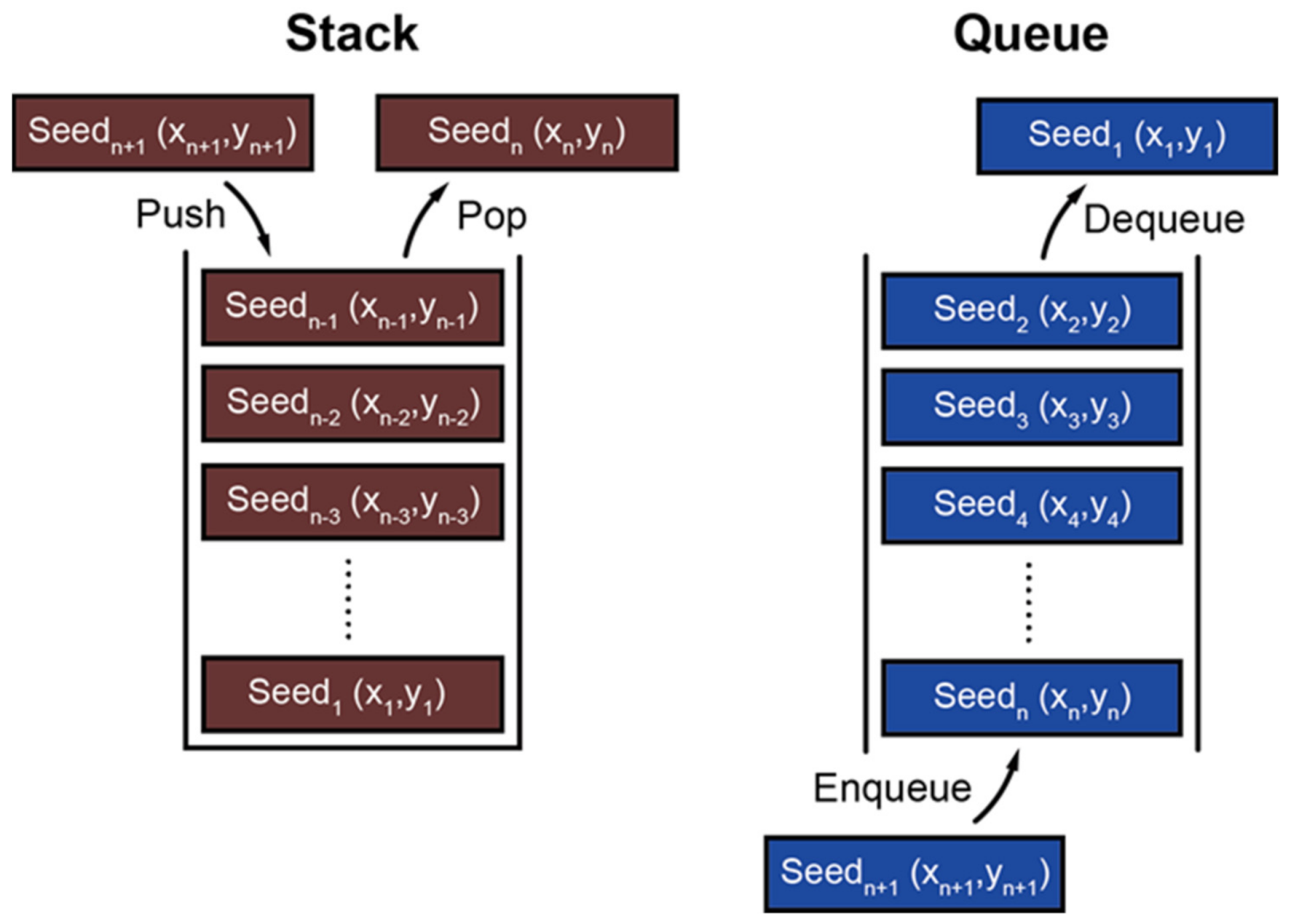
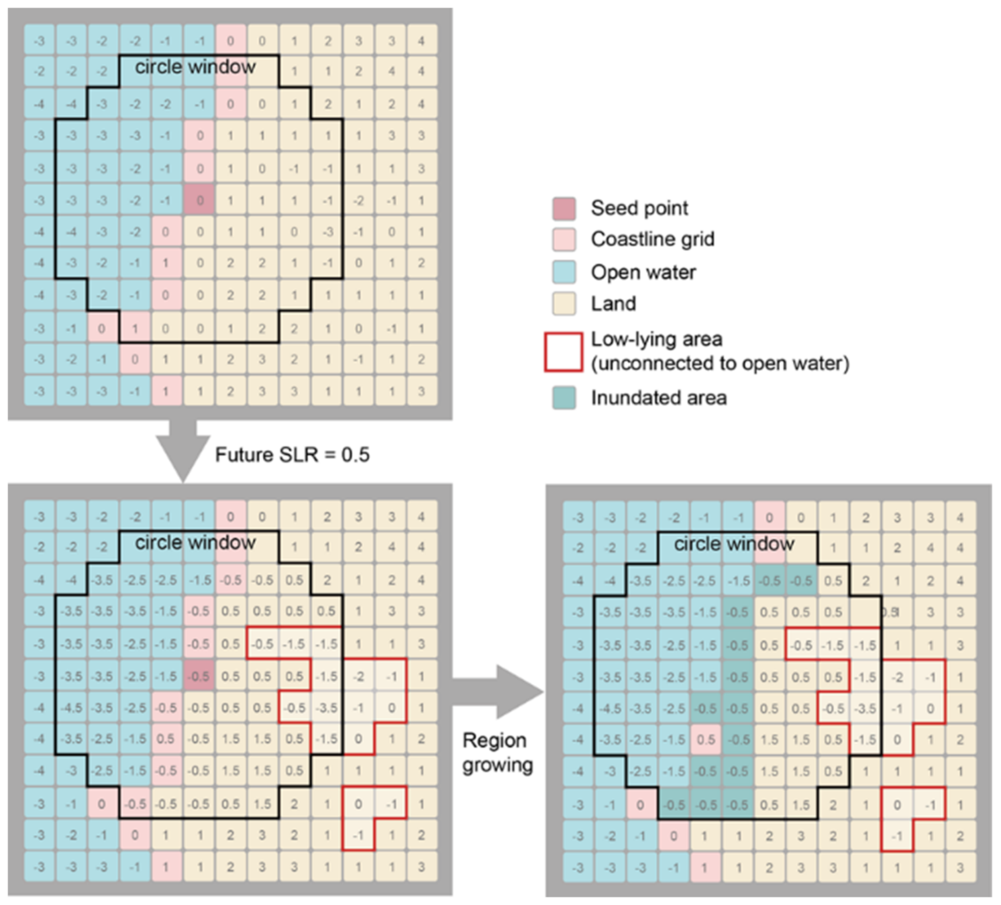
3.1. Region Growing Algorithm

Region growing, also called the flood-fill algorithm, is a region-based image segmentation algorithm to partition the image into regions that represent the same attribute by spatial continuity [25]. The region growing algorithm is an algorithm based on the expansion of the spatial position of the pixel, so the local color histogram is introduced in the region growing algorithm, so that statistical characteristics of the local color of the pixel can be effectively combined with spatial pixel location information. In the case of image segmentation, the general criteria for achieving good segmentation results are that the similarity of pixels in the same region is greater than the similarity between different pixel regions. Seeds of regional growth should, on the basis of this criteria, comply with highly similar features between the pixels and their neighbors [43]. This algorithm has been widely used in the “bucket” fill-tool of raster graphics editor programs (photoshop, paint, etc.). The region growing algorithm takes three parameters: a seed point, a started value, and a replacement value. The basic approach is to select a set of initial seed points based on the user’s preferences; then, the extent of the region is grown from these seed points to adjacent points by checking whether the attribute of that point meets the criteria. If the point is eligible for growing, we classify it into the seed points and change the value to the replacement value. Then, the process is iterated, which looks for all points that are connected to the initial seed point until every point in the region containing the seed point is visited.

To implement this approach, the waiting list of pixels makes use of a queue or stack data structure. Both queue and stack are abstract data types, which serves as a collection of elements and the operations to add and remove the elements. The main difference between these two data structures are the direction to access the element that removes the element from the same side or another side of the input element (as shown in Figure 4), which are called the Last-In-First-Out (LIFO) and First-In-First-Out (FIFO) structure, respectively [23].

Therefore, the region growing algorithm highly depends on the criteria used to decide whether a cell should be contained in the region or not, the connectivity type used to determine the neighbors, and the strategy to visit the adjacent cells.

However, sea level varies by location, as well as HAT changes with location owing to currents, winds, and bathymetry. Therefore, the modified region growing algorithm was developed in response to the variations of sea level by operating the algorithm on every coastline grid in the loop. The following equation describes how the approach is used to estimate the coastal flooding, which is modified from [27]:

$$F_{x,y}^i=\{\begin{array}{c}{S}_i, E_{x,y}\le S_i and F_{x,y}^{i-1}\le S_i\\ F_{x,y}^{i-1},E_{x,y}\le S_i and F_{x,y}^{i-1}>S_i,C\\ 0,E_{x,y}> S_i\end{array}$$

(4)

where F_x,y is a real number, representing the inundation depth of flood at location (x, y), either a positive number depicts the new flooded depth (S_i) or previous flood depth c, or not flooded (0), E_x,y is DEM elevation at location (x, y), S_i is the water level of coastline cell i, and C is connectivity, which is (1) for connected and (0) for unconnected. F⁰_x,y are set as 0 and Fⁱ_x,y is updated when each S_i is applied.

The algorithm runs over all coastline grids as the seed points, operating in the particular circle extent, which is set to a 50-km radius as the farthest spreading area of the flood from a given seed point. In the circle windows of specific coastline grid i, the DEM cell (x, y) will be considered as flooded only if the elevation of this cell is lower than the projected sea level at coastline grid i and is connected to this seed point according to the connectivity rules. The flooded depth will be renewed if the sea level at this seed is higher than the inundation result from the growing process of previous seeds.

Figure 5 shows the procedure of the modified region growing algorithm proposed in this study. The future SLR is subtracted from the DEM cell within the circle window extent of the seed point to generate the possible flooding map. After performing the region growing algorithm, we can get the inundated area in dark blue. The new inundated area is selected as seed points, and we use the region growing algorithm to search the inundated area until no change occurs. The DEM cells with values under elevation 0 in the red polygon are not considered as the inundation area, because these pixels are not connected to previously inundated cells.

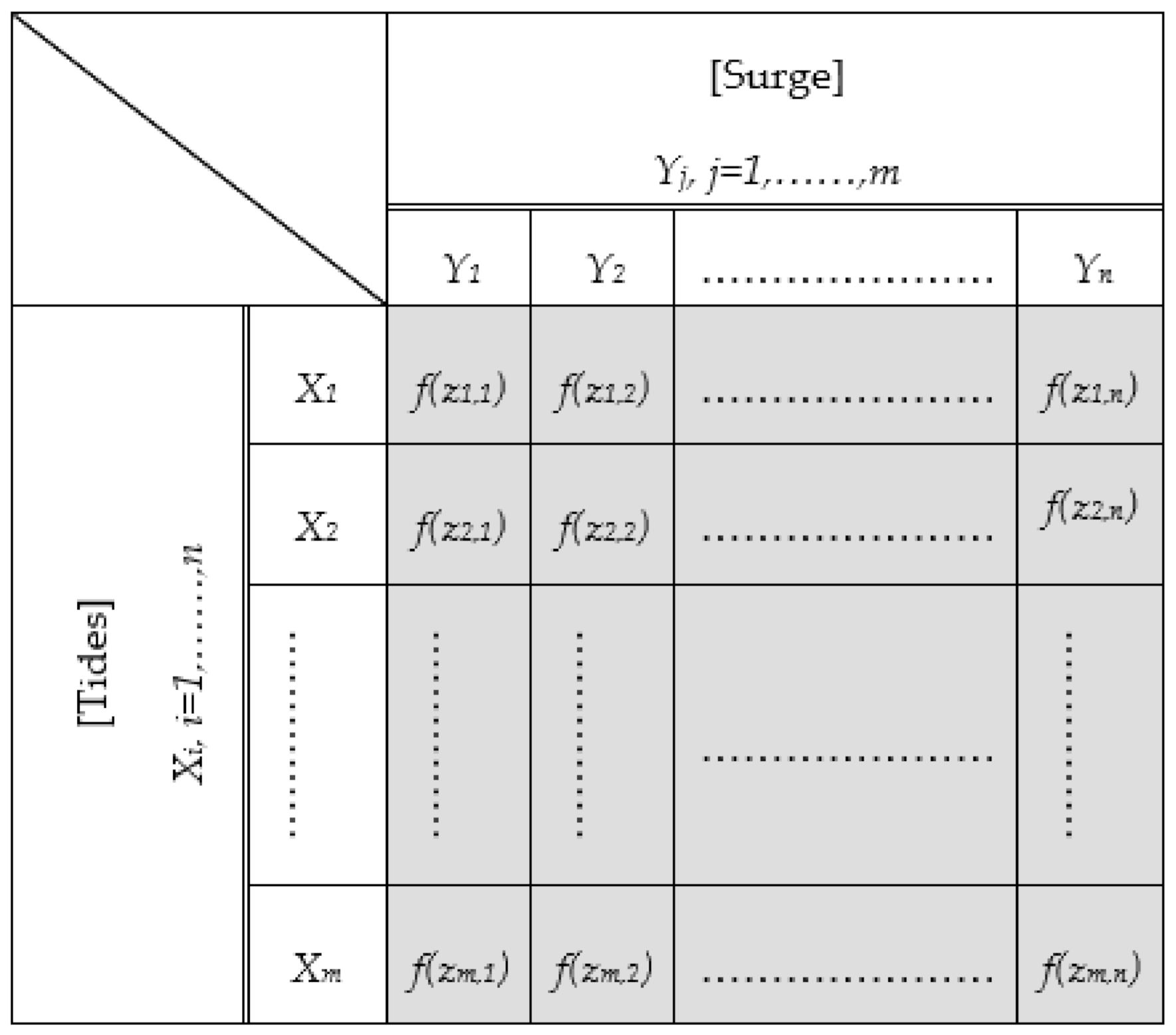
3.2. Probability of Exceedance and Return Periods

The primary goal of extreme flood level analysis is to predict the likelihood of an event occurring in the future. The probability of exceedance (p), which is the chance of a flood level being exceeded in any one time period, or the return period (T_R), which is the average number of time intervals between the occurrence of events equal to or greater than a given flood level, can be used to estimate the predicted probability of occurrence of an event. Then, T_R is the opposite of p.

To obtain p and T_R, f(x) is assumed to be the probability density function for the variable of interest (x). Then, f(x) represents the cumulative distribution function for this variable. The probability that x will not exceed an extreme event (z) in any one time period is presented by:

$$\mathrm{F}\left(\mathrm{z}\right)={{\displaystyle \int }}_{-\infty }^{\mathrm{z}}\mathrm{f}\left(\mathrm{x}\right)\mathrm{dx}.$$

(5)

The probability of z being exceeded in any given year, or the probability of exceedance (p(z)) is also described as:

$$\mathrm{p}\left(\mathrm{z}\right)=1-\mathrm{F}\left(\mathrm{z}\right)={{\displaystyle \int }}_{\mathrm{z}}^{\infty }\mathrm{f}\left(\mathrm{x}\right)\mathrm{dx}.$$

(6)

Furthermore, the return period of z, denoted as T_R(z), is the opposite of p(z) [29,41]:

$${\mathrm{T}}_{\mathrm{R}}\left(\mathrm{z}\right)=\frac{1}{\mathrm{p}\left(\mathrm{z}\right)}=\frac{1}{1-\mathrm{F}\left(\mathrm{z}\right)}.$$

(7)

The variable, x, could reflect either sea level or wave height. As a consequence, the value z reflects the extreme flood level or extreme wave height. The magnitude of the extreme flood or extreme wave situation, z, is associated with a specific exceedance probability p(z) and return time T_R(z).

The importance of providing reliable forecasts of extreme sea levels increased the need for more accurate estimations as well as the potential to use shorter data series [30]. The JPM was developed by Pugh and Vassie [29] to fulfill these two objectives.

The three main components of sea level variations considered in the JPM are the mean sea level Z₀(t), tidal level X(t), and meteorologically induced level Y(t). The mean sea level corresponds to long-term fluctuations caused by climatologic and geologic impacts, and it can be defined using standard regression of the long-term record of observed sea level. However, this term is usually assigned a constant or a zero value, because it is generally small compared with tidal and meteorologically induced levels [12].

$$\mathsf{\zeta }\left(\mathrm{t}\right)={\mathrm{Z}}_0\left(\mathrm{t}\right)+\mathrm{X}\left(\mathrm{t}\right)+\mathrm{Y}\left(\mathrm{t}\right)$$

(8)

With the availability of observed sea level $\mathsf{\zeta }\left(\mathrm{t}\right)$ and tide data (X(t)), and an assumption of Z₀(t) = 0, the storm surge can be described as:

$$\mathrm{Y}\left(\mathrm{t}\right)=\mathsf{\zeta }\left(\mathrm{t}\right)-\mathrm{X}\left(\mathrm{t}\right).$$

(9)

If the probability density function of storm surges is f(y), the probability density function of tides can be represented by ${\mathrm{f}}_{\mathrm{T}}\left(\mathsf{\zeta }-\mathrm{y}\right)$. Since the JPM assumes that tides and storm surges are independent, the probability density function of the total sea level can be expressed as [29]:

$$\mathrm{f}\left(\mathsf{\zeta }\right)={{\displaystyle \int }}_{-\infty }^{\infty }{\mathrm{f}}_{\mathrm{T}}\left(\mathsf{\zeta }-\mathrm{y}\right){\mathrm{f}}_{\mathrm{s}}\left(\mathrm{y}\right)\mathrm{dy}.$$

(10)

Then, the cumulative density function, $\mathrm{F}\left(\mathsf{\zeta }\right)$, for a given extreme sea level, z, is expressed as:

$$\mathrm{F}\left(\mathrm{z}\right)={{\displaystyle \int }}_{-\infty }^{\mathrm{z}}\mathrm{f}\left(\mathsf{\zeta }\right)\mathrm{d}\mathsf{\zeta }.$$

(11)

Given the cumulative density function of the sea level, any probability of exceedance and return period can be obtained by applying Equations (7) and (8).

In the case of 6 min data records, the JPM is used to estimate the sample probability density functions for each contributing factor in Equation (11), to estimate the 6 min joint probability of exceedance based on these, and to use the 6 min joint probability of exceedance to estimate the annual joint probability of exceedance. The corresponding return period may also be determined based on Equation (8). Since the JPM can be applied for data collected for short time intervals, it can be used in cases with short data records, on the order of years, provided that there are sufficient and accurate data records within those years.

Assuming availability of 6 min tides and observed sea levels, the process of estimating the 6 min joint probability of exceedance begins with compiling the time series of 6 min tides and storm surges.

Then, the time series of tides X(t) and storm surges Y(t) are used to construct histograms for the tides and storm surges. With reference to Figure 6, for N data points, n intervals for tides (X), and m intervals for storm surges (Y), the relative frequencies, f, in the highlighted cells represent the probabilities of occurrence of tides and storm surges for the given intervals.

Applying Equation (11), the product of the sample probability density functions of tides and storm surges yields the sample joint probability density function of tides and storm surges, which are used in Equation (12) to determine the sample joint cumulative density function and the sample joint probability of exceedance based on Equation (7). Denoting the sample joint probability of exceedance as ${\mathrm{P}}_{\mathrm{N}}\left(\mathrm{z}\right)$, the joint probability of exceedance, ${\mathrm{P}}_1\left(\mathrm{z}\right)$, is determined as:

$${\mathrm{P}}_{\mathrm{N}}\left(\mathrm{z}\right)=1-{[1-{\mathrm{P}}_1\left(\mathrm{z}\right)]}^{\mathrm{N}}$$

(12)

where z is total sea level, and N is the total number of data recorded over time. If N is a large number, Equation (13) can be approximated as:

$${\mathrm{P}}_{\mathrm{N}}\left(\mathrm{z}\right)\approx 1-\exp \left[-{\mathrm{Np}}_1\left(\mathrm{z}\right)\right].$$

(13)

If the values of sea levels exhibit persistence (i.e., dependence between values in adjacent time periods), the 6 min probability of exceedance may be adjusted. The JPM has been adapted based on the assumption of one-dependence, which implies that the probability density function of each sea level depends only on the value of the previous sea level [29]. Here, the 6 min joint probability of exceedance in a set of N samples can be determined by solving the following equation:

$${\mathrm{P}}_{\mathrm{N}}\left(\mathrm{z}\right)=1-\exp [-{\mathrm{Np}}_1\left(\mathrm{z}\right)\left(1-\frac{P_2\left(z\right)}{P_1\left(z\right)}\right)$$

(14)

where ${\mathrm{P}}_2\left(\mathrm{z}\right)$ is the probability of exceeding z in two successive time periods and can be determined by constructing the histograms based on two-6 min intervals. The ultimate goal of the JPM is to determine the annual joint probability of exceedance and return period in years. Thus, the relationship between the annual joint probability of exceedance and the 6 min joint probability of exceedance needs to be established. If $p_{\gamma }\left(z\right)$ is defined as the annual joint probability of exceedance, $p_{\gamma }\left(z\right)$ can be described as a function of ${\mathrm{p}}_1\left(\mathrm{z}\right)$ [29]:

$$p_{\gamma }\left(z\right)=1-\exp \left[-87,660{\mathrm{p}}_1\left(\mathrm{z}\right)\alpha \right]$$

(15)

where $\alpha =1$ for independent 6 min sea level and $\alpha$ = $\left(1-\frac{P_2\left(z\right)}{P_1\left(z\right)}\right)$ for dependent 6 min sea levels. Tawn and Vassie [30] found that the assumption might be false but led only to a small overestimation of return levels. In other words, the short-term intervals of water levels may not be fully independent, as assumed in the joint probability method, but extreme levels may be only weakly dependent. Pugh and Vassie [29] also indicate that the adjustment for correlation $\left(1-\frac{P_2\left(z\right)}{P_1\left(z\right)}\right)$ is so small compared with the uncertainties from other causes that in view of the accuracy required in practice, it is not required.

The JPM application is valid under a few assumptions. Except in shallow water where there is a significant tide and storm surge interaction, the assumption of the independent relationship between tides and storm surges is usually true [30]. In order to satisfy this assumption, Pugh and Vassie [29] suggested finding the storm surge distributions for each interval of tides, which increases the computation time, and is not applicable in the cases with more than two dependent variables. The other assumption is that the density function of storm surges over a given period should represent the probability density function for all of the storm surges. This is the key to the stability of the JPM and must hold if the tidal and storm surge probabilities are to be combined to calculate the probabilities of total sea levels as described by Equation (11) [29,41].

4. Results and Analysis

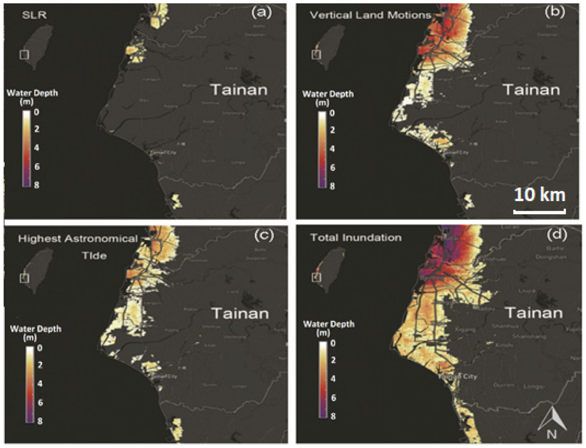
4.1. Flood Risk Map

Several important regional factors that may result in the coastal inundation of Tainan city have been selected, including future sea level rise, vertical land motions, HAT, and the flood risk estimation. The water depths (or inundation height) along the coastline are estimated by the sea level data derived from satellite altimetry, uplift and subsidence rate from leveling and GPS, and tide height from the regional tidal model, respectively. The basic concept of generation of flooding area is using DEM and the predicted water depth in the future by the region growing algorithm. By subtracting the inundation height from the DEM, the DEM cells with negative elevation value represent the area that will be inundated in the future.

The coastal inundation situations in this study are as follows: (1) Sea level rise situation: The water depth in the future of the SLR situation is simulated by applying Equation (4), which combines the values of MSL at 2012, the discrepancy between two reference ellipsoids, and the amount of SLR in 100 years. Figure 7a presents the sea level at 2112, demonstrating that the long-term SLR over 100 years is higher at the Beimen coastline than in other regions. (2) VLM situation: In this situation, instead of predicting the future sea level along the coastline, the DEM at 2112 was generated by subtracting the VLM from the present DEM_t(0). The VLMs are also derived from multiplying the annual subsidence rates in meters and 100-year predictions. So, the DEM at 2112 in response to vertical land motions can be expressed as:

$$DE{M}_{t\left(x\right)}=DE{M}_{t\left(0\right)}-\left(s\times \left(t_x-t_0\right)\right)$$

(16)

DEM_t(x) is the DEM in reference year t_x, DEM_t(0) is the DEM in reference year t₀, and “s” is the VLM trend in meters, and it is considered as constant in a grid but spatially different. We assume that the VLM is linear and computed using 50 GPS continuous stations and 510 precise leveling point data from 2000 to 2008.

Figure 7b presents the terrain elevation at 2012 and shows high VLM in the Beimen, Jiangiu, and Qiqu districts. (3) HAT situation: The HAT is generated by the Taiwan tidal model TWN5N proposed by The Industrial Technology Research Institute, Taiwan. The model outputs the HAT height referring to MSL over the 18.6-year tidal cycle along the Taiwan coastline, which could act as the input data of the region growing algorithm directly, as shown in Figure 7c. (4) Total situation: With sea level and land elevation data shown above, the coastal inundation at 2012 under different situations is estimated and results are depicted in Figure 7d. In the total inundation situation, all inundation factors are taken into account. However, the inundation area is not simply estimated by adding the simulation result (inundation water depth) of three factors on every cell together.

Compared to other situations, VLMs have the largest inundation area with the maximum inundation depth (4–5 m) and mean depth (≈3 m), implying the most severe situation. On the other hand, SLR situation shows the least serious situation in three simulated conditions.

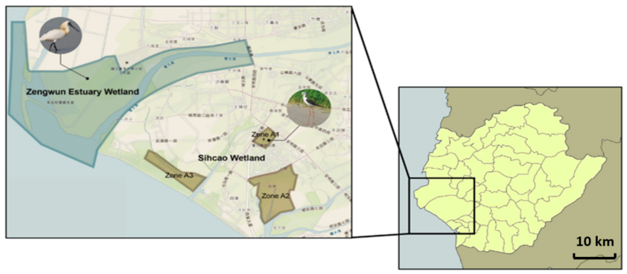
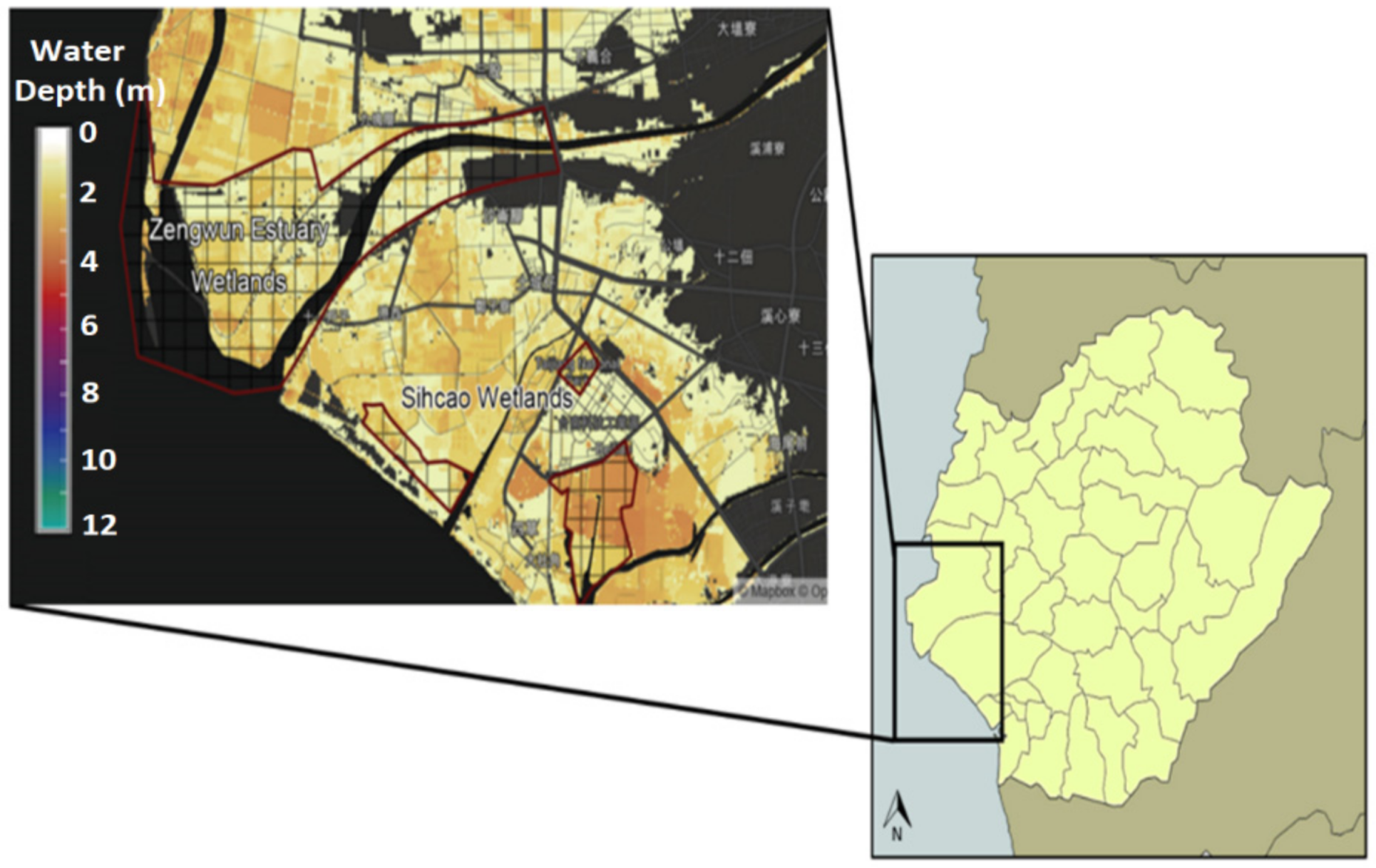
4.2. Wetlands Loss in Tainan

The southeastern coastal region encompasses vast areas of wetland habitat important to wildlife and other economically valuable natural resources.

Table 3. The percentages of wetland loss under different drivers of risk over 100 years.

Name	SLR(%)	VLM 1 (%)	HAT(%)	Total Inundation (%)
Zengwun Estuary	6.42	21.50	19.90	88.51
Sihcao	0.32	89.16	58.77	99.47
Bajhang Estuary	5.10	99.99	91.66	100
Beimen	69.45	99.33	97.82	99.77
Cigu Salt Pan	0.60	66.46	73.59	98.98
Yanshuei Estuary	5.32	90.57	87.82	96.97

¹ Vertical land motions.

demonstrates the percentages of the wetland loss of national and international importance in Tainan. Almost all the Tainan wetlands are exposed to be inundated. Based on Table 3, the percentage of total wetlands loss under SLR situations is about 14.5%, while there is 77.8% loss under the VLMs situation, 71.6% loss under the HAT situation, and 97.35% loss of wetlands under the combined situation. That is to say, if three hypothetical situations all happen in the future, coastal wetlands of national importance in Taiwan will almost disappear, including two wetlands of international importance (Figure 8). It is noted that while the wetland loss due to the HAT is recurrent, wetland loss as a result of SLR and VLM could be permanent. The mean sea level and VLM changes could result in a higher risk of flooding in coastal zones, the intrusion of seawater, and loss of important wetlands, industrial parks and several residential areas near old Tainan City with social, economic, and environmental consequences.

4.3. Extreme Sea Levels

In addition to the analysis of static flooding in the near future, an evaluation of the possibility of extreme sea levels is important for the design of modern coastal infrastructure systems. Scientists analyzed flooding risks from observations using probability and statistical approaches to predict the effects of extreme sea levels.

By performing the tidal analysis, we can obtain the separated tide with considering the long-term SLR and surge components. Then, the DJPM is applied to the tide and surge level data to obtain the joint probability distribution. Therefore, the extreme flood estimation is derived from the integration of joint probability function and the conversion of time unit of probabilities. Figure 9 and

Table 4. The estimation of extreme sea level of tide-gauge stations.

		Extreme Sea Level [m]
Return Period (year)	Boziliao	Jiangjun	Kaohsiung
100	1.43	0.76	0.55
500	1.62	0.90	0.70
1000	1.70	0.95	0.75
		Extreme Sea Level with Long-Term SLR (m)
100	1.67	0.97	0.77
500	1.86	1.10	0.92
1000	1.93	1.15	0.97

represent the estimation of extreme sea level of tide-gauge stations selected in this study. The extreme sea level at the north part of Tainan is relatively larger than those at the others.

The 100-year flood risk at the end of 21st century in Tainan city was also assessed in this study. The seed points are selected from the lowest point of each city by using the DEM that is considering vertical land motion. The initial inundation depth of seed points are the extreme sea level with considering local long-term SLR from the nearest tide-gauge station. Figure 10 represents the flood risk map of the Tainan. The north part of Tainan has the largest inundation area percentage in this city with 379.94 km depicting, which means about 16.82% of the city is flooded by a 1 in 100-year level (and this 1 in 100-year level may become a 1 in 20-year flood due to SLR and other combined effects).

To present the land use categories that will be influenced by the total inundation situation, we applied the land use data provided by the National Land Surveying and Mapping Center (NLSC), Ministry of the Interior, Taiwan on the inundation area of the extreme flood in Tainan. The data are investigated and produced from 2006 to 2015. Lands are classified into nine land use categories, including agriculture, forest, transportation, water conservation, building, government, recreation, mine, and others.

Figure 11 shows the land use map of the inundated area. Most of the inundation areas are agricultural land use (60% of total inundation area of Tainan). The second largest land use type is water conservation (about 13% of total inundation area of Tainan), including several rivers and oyster farming at Cigu Lagoon. The third largest type is “others”, because wetlands were classified into this category, including two important wetlands, Zengwun Estuary Wetland and Sihcao Wetland, which are almost flooded. The building land use type colored in red is mainly located at Tainan Technology Industrial Park and Anping Industrial Park with several residential areas.

5. Discussion and Conclusions

Coastal flooding poses serious risks to coastal areas and, owing to environmental and socio-economic changes, the vulnerability of coastal communities and economic sectors to flooding will increase in the coming decades. It is widely recognized that city vulnerability estimates are critical for the preparation of adaptation steps. The simulation of static flooding situation and the estimation of extreme sea level of the southwest coast of Taiwan (Tainan city) at 2112 was conducted in this study. By using the DEM, regional sea level changes reconstructed from altimetry data, VLMs derived from leveling and GPS data, and ocean tides from the regional Taiwan tidal Model TWN5T, we evaluated several factors contributing to the risk of flooding in Tainan, including SLR, VLMs, HAT, and the combined situations.

The results suggest that Tainan suffers from severe floods with an inundation area that includes about 16.8% of the city. Budai and Beimen districts (northern districts) are very susceptible to coastal inundation. The maximum inundation depth occurs at these two districts reclaimed land (≈8 m depth), which is due to the negative elevation below sea level, and the subsidence rate of −90 mm/yr is also larger than other places in Tainan. The main reason why this area is suffering from coastal flooding is the serious subsidence rate, where similar results can be seen in the inundation map under the situation of VLMs. The range of inundation depth around Tainan area is 0–8 m depth with a mean value of 4 m. At the municipal scale, Tainan city suffers from serious coastal inundation where sea level intrudes 18 km inland through Beimen, Xuejia, and Madou Dist. In addition, important wetlands, industrial parks, and several residential areas near old Tainan City are flooded under the combined situation.

Seawater inundation especially leads to the loss of western coastal wetland. As shown in Figure 8, 88.5% of Zengwun Estuary Wetlands and 99.5% of Sihcao Wetlands, the important Black-faced Spoonbills (Platalea minor) Refuge, will disappear. During the winter season, over half of the black-faced spoonbill population migrates to these two wetlands. Therefore, the loss of Zengwun Estuary Wetlands and Sihcao Wetlands could cause habitat loss and subsequently the extinction of this endangered species of migratory birds.

To have a better understanding of risk zones, land use data of Tainan on the inundation area was applied. Most of the inundation area are agricultural land use (60% of total inundation area of Tainan). Except for the combined situations, the vertical land motions situation has the largest inundation area as well as maximum inundation depth and mean depth, which implies it is the most severe situation.

The extreme sea level was evaluated by the direct joint probability method using records of three tide-gauge stations around Tainan where the result suggests that the extreme sea level at the northern coastal area of Tainan is relatively larger. The overall findings indicate that not only the combined effect of SLR, VLMs, and tides but also the extreme sea level would impact on the vulnerability of the coastal area dramatically. A broad range of area will suffer from inundation in future.

Limitations and Future Work

A reliable rapid assessment methodology is useful for the development of coastal flood adaptation, as it helps planners determine the efficacy of interventions against projections of flood impacts. The approach proposed in this study enables us, in the face of uncertainty, to quantify the impacts of combined environmental changes and to promote the identification of critical points above which significant increases in exposure to harm can be expected. In addition, the evaluation of the situation enables us to analyze the effect of changes in various factors relative to each other in the case of Tainan City, thereby illustrating the need for more study and adaptation in the field of land subsidence.

The risk assessment of flooding areas is also potentially useful for the coastal ocean and land management plans to develop an appropriate adaptation policy for preventing disasters resulting from global climate change. In order to build robust adaptation pathways, policy makers and local authorities need to have a clear view of systemic risks affecting human health and safety, the environment, the economy, and society at large. However, the flooding risk assessment in the current study was performed by only considering the physical factors and their linear trend. In order to estimate the exposure to the hazard, more social–economic data such as the population and economic value of the land use should be included in the analysis. Furthermore, the effect of wave run-up should be considered when estimating the extreme sea levels in the western coastal area because wave run-up will cause a significant rise of sea level at the shallow shoreline area. Moreover, even if subsidence is an important factor for the assessment of future inundation risk, especially for the low-lying coastal plains of western Taiwan, this factor could not be considered in the present analysis due to the lack of homogeneous data mapping the phenomenon for the overall coast of study area.

Additionally, the actual damage that would occur as a result of each inundation situation might not be exactly the same as predicted, since it is also depends on other factors, such as flow velocity, flood mitigation measures, and sediment load.

A more accurate understanding of the distribution of the elements at risk across space and time (e.g., land use, population, and infrastructure dynamics) and of their vulnerability should be established for future improvements to the proposed approach. Future research should consider how different management options will contribute to reducing the overall multi-risk score and cascading uncertainties in space and time, in order to provide comprehensive science-based outputs for decision-making from a multi-risk perspective and better support decision-making processes to evaluate the effectiveness of various adaptation pathways.

References

1. Gesch, D.B. Analysis of Lidar Elevation Data for Improved Identification and Delineation of Lands Vulnerable to Sea-Level Rise. J. Coast. Res. 2009, 10053, 49–58. [Google Scholar] [CrossRef]
2. Rahmstorf, S. Sea-level rise: Towards understanding local vulnerability. Environ. Res. Lett. 2012, 7, 021001. [Google Scholar] [CrossRef]
3. Jevrejeva, S.; Grinsted, A.; Moore, J.C. Upper limit for sea level projections by 2100. Environ. Res. Lett. 2014, 9, 104008. [Google Scholar] [CrossRef] [Green Version]
4. McGranahan, G.; Balk, D.; Anderson, B. The rising tide: Assessing the risks of climate change and human settlements in low elevation coastal zones. Environ. Urban. 2007, 19, 17–37. [Google Scholar] [CrossRef]
5. Prasetyo, Y.; Bashit, N.; Sasmito, B.; Setianingsih, W. Impact of Land Subsidence and Sea Level Rise Influence Shoreline Change in The Coastal Area of Demak. IOP Conf. Ser. Earth Environ. Sci. 2019, 280, 012006. [Google Scholar] [CrossRef]
6. Tseng, Y.-H.; Breaker, L.C.; Chang, E.T.-Y. Sea level variations in the regional seas around Taiwan. J. Oceanogr. 2010, 66, 27–39. [Google Scholar] [CrossRef]
7. Hu, C.-K.; Chiu, C.-T.; Chen, S.-H.; Kuo, J.-Y.; Jan, S.; Tseng, Y.-H. Numerical Simulation of Barotropic Tides around Taiwan. Terr. Atmos. Ocean. Sci. 2010, 21, 71. [Google Scholar] [CrossRef] [Green Version]
8. IPCC. Climate Change: The Physical Science Basis: Working Group I Contribution to the Fourth Assessment Report of the IPCC; Cambridge University Press: Cambridge, UK; New York, NY, USA, 2007. [Google Scholar]
9. Wunsch, C.; Ponte, R.M.; Heimbach, P. Decadal Trends in Sea Level Patterns: 1993–2004. J. Clim. 2007, 20, 5889–5911. [Google Scholar] [CrossRef]
10. Ward, P.J.; Marfai, M.A.; Yulianto, F.; Hizbaron, D.R.; Aerts, J.C.J.H. Coastal inundation and damage exposure estimation: A case study for Jakarta. Nat. Hazards 2010, 56, 899–916. [Google Scholar] [CrossRef] [Green Version]
11. Davis, K.F.; Bhattachan, A.; D’Odorico, P.; Suweis, S. A universal model for predicting human migration under climate change: Examining future sea level rise in Bangladesh. Environ. Res. Lett. 2018, 13, 064030. [Google Scholar] [CrossRef]
12. Tsimplis, M.N.; Woodworth, P.L. The global distribution of the seasonal sea level cycle calculated from coastal tide gauge data. J. Geophys. Res. Space Phys. 1994, 99, 16031–16039. [Google Scholar] [CrossRef]
13. Teng, W.-H.; Hsu, M.-H.; Wu, C.-H.; Chen, A.S. Impact of Flood Disasters on Taiwan in the Last Quarter Century. Nat. Hazards 2006, 37, 191–207. [Google Scholar] [CrossRef] [Green Version]
14. Ching, K.-E.; Hsieh, M.-L.; Johnson, K.M.; Chen, K.-H.; Rau, R.-J.; Yang, M. Modern vertical deformation rates and mountain building in Taiwan from precise leveling and continuous GPS observations, 2000–2008. J. Geophys. Res. Space Phys. 2011, 116, 116. [Google Scholar] [CrossRef]
15. Lan, W.-H.; Kuo, C.-Y.; Kao, H.-C.; Lin, L.-C.; Shum, C.K.; Tseng, K.-H.; Chang, J.-C. Impact of Geophysical and Datum Corrections on Absolute Sea-Level Trends from Tide Gauges around Taiwan, 1993–2015. Water 2017, 9, 480. [Google Scholar] [CrossRef]
16. Ge, X.; Li, T.; Zhang, S.; Peng, M. What causes the extremely heavy rainfall in Taiwan during Typhoon Morakot (2009)? Atmos. Sci. Lett. 2010, 11, 46–50. [Google Scholar] [CrossRef]
17. Krestenitis, Y.N.; Androulidakis, Y.S.; Kontos, Y.N.; Georgakopoulos, G. Coastal inundation in the north-eastern mediterra-nean coastal zone due to storm surge events. J. Coast. Conserv. 2011, 15, 353–368. [Google Scholar] [CrossRef]
18. Perini, L.; Calabrese, L.; Salerno, G.; Ciavola, P.; Armaroli, C. Evaluation of coastal vulnerability to flooding: Comparison of two different methodologies adopted by the Emilia-Romagna region (Italy). Nat. Hazards Earth Syst. Sci. 2016, 16, 181–194. [Google Scholar] [CrossRef] [Green Version]
19. Torres, J.M.; Bass, B.; Irza, N.; Fang, Z.; Proft, J.; Dawson, C.; Kiani, M.; Bedient, P.B. Characterizing the hydraulic interactions of hurricane storm surge and rainfall–runoff for the Houston–Galveston region. Coast. Eng. 2015, 106, 7–19. [Google Scholar] [CrossRef] [Green Version]
20. Passeri, D.L.; Hagen, S.C.; Plant, N.G.; Bilskie, M.V.; Medeiros, S.C.; Alizad, K. Tidal hydrodynamics under future sea level rise and coastal morphology in the Northern Gulf of Mexico. Earth’s Futur. 2016, 4, 159–176. [Google Scholar] [CrossRef] [Green Version]
21. Bilskie, M.V.; Hagen, S.C.; Medeiros, S.C.; Passeri, D.L. Dynamics of sea level rise and coastal flooding on a changing land-scape. Geophys. Res. Lett. 2014, 41. [Google Scholar] [CrossRef]
22. Doong, D.-J.; Lo, W.; Vojinovic, Z.; Lee, W.-L.; Lee, S.-P. Development of a New Generation of Flood Inundation Maps—A Case Study of the Coastal City of Tainan, Taiwan. Water 2016, 8, 521. [Google Scholar] [CrossRef] [Green Version]
23. Bins, L.S.a.; Fonseca, L.M.G.; Erthal, G.J.; Ii, F.M. Satellite imagery segmentation: A region growing approach. Simpósio Bra-Sileiro Sens. Remoto 1996, 8, 677–680. [Google Scholar]
24. Dalvand, M.; Fathi, A.; Kamran, A. Flooding region growing: A new parallel image segmentation model based on membrane computing. J. Real-Time Image Process. 2021, 18, 37–55. [Google Scholar] [CrossRef]
25. Adams, R.; Bischof, L. Seeded region growing. Pattern Analysis and Machine Intelligence. IEEE Trans. 1994, 16, 641–647. [Google Scholar]
26. Matgen, P.; Hostache, R.; Schumann, G.; Pfister, L.; Hoffmann, L.; Savenije, H. Towards an automated SAR-based flood mon-itoring system: Lessons learned from two case studies. Phys. Chem. Earth Parts A/B/C 2011, 36, 241–252. [Google Scholar] [CrossRef]
27. Poulter, B.; Halpin, P.N. Raster modelling of coastal flooding from sea-level rise. Int. J. Geogr. Inf. Sci. 2008, 22, 167–182. [Google Scholar] [CrossRef]
28. Bittermann, K.; Rahmstorf, S.; Perrette, M.; Vermeer, M. Predictability of twentieth century sea-level rise from past data. Environ. Res. Lett. 2013, 8, 014013. [Google Scholar] [CrossRef]
29. Pugh, D.; Vassie, J. Applications of the joint probability method for extreme sea level computations. Proc. Inst. Civ. Eng. 1980, 69, 959–975. [Google Scholar] [CrossRef]
30. Tawn, J.; Vassie, J.; Gumbel, E. Extreme sea levels: The joint probabilities method revisited and revised. Proc. Inst. Civ. Eng. 1989, 87, 429–442. [Google Scholar] [CrossRef]
31. Liu, J.C.; Lence, B.J.; Isaacson, M. Direct Joint Probability Method for Estimating Extreme Sea Levels. J. Waterw. Port. Coastal. Ocean Eng. 2010, 136, 66–76. [Google Scholar] [CrossRef] [Green Version]
32. Lin, K.-C.; Hu, J.-C.; Ching, K.-E.; Angelier, J.; Rau, R.-J.; Yu, S.-B.; Tsai, C.-H.; Shin, T.-C.; Huang, M.-H. GPS crustal deformation, strain rate, and seismic activity after the 1999 Chi-Chi earthquake in Taiwan. J. Geophys. Res. Space Phys. 2010, 115, 115. [Google Scholar] [CrossRef] [Green Version]
33. Yin, J.; Yin, Z.; Wang, J.; Xu, S. National assessment of coastal vulnerability to sea-level rise for the Chinese coast. J. Coast. Conserv. 2012, 16, 123–133. [Google Scholar] [CrossRef]
34. Tainan Government Boreau. Available online: https://www.tainan.gov.tw/en/News_Content.aspx?n=13207&s=1395588 (accessed on 22 March 2021).
35. Taiwan’s wetland. Available online: https://wetland-tw.tcd.gov.tw/en/index.php (accessed on 14 September 2016).
36. Liu, C.-S.; Liu, S.-Y.; Lallemand, S.E.; Lundberg, N.; Reed, D.L. Digital Elevation Model Offshore Taiwan and Its Tectonic Implications. Terr. Atmos. Ocean. Sci. 1998, 9, 705–738. [Google Scholar] [CrossRef]
37. The altimeter products were produced by Ssalto/Duacs and distributed by Aviso+, with support from Cnes. Available online: https://www.aviso.altimetry.fr (accessed on 14 April 2015).
38. Sue, W.S.; Kuo, C.Y.; Shum, C.K. Monitoring of Sea Level Rise around Taiwan using Satellite Altimetry and Tide Gauge. In Proceedings of the EGU General Assembly 2010, Vienna, Austria, 2–7 May 2010. [Google Scholar]
39. Wöppelmann, G.; Marcos, M. Vertical land motion as a key to understanding sea level change and variability. Rev. Geophys. 2016, 54, 64–92. [Google Scholar] [CrossRef] [Green Version]
40. Church, J.A.; Clark, P.; Cazenave, A.; Gregory, J.; Jevrejeva, S.; Levermann, A.; Merrifield, M.; Milne, G.; Nerem, R.S.; Nunn, P.; et al. Sea level change. In Climate Change 2013: The Physical Science Basis; Stocker, T.F., Qin, D., Plattner, G.-K., Tignor, M., Allen, S., Boschung, J., Nauels, A., Xia, Y., Bex, V., Midgley, P., et al., Eds.; Cambridge University Press: Cambridge, UK; New York, NY, USA, 2014. [Google Scholar]
41. Pugh, D.; Woodworth, P. Sea-Level Sciencei; Cambridge University Press: Cambridge, UK, 2014. [Google Scholar]
42. Chen, K.-H.; Yang, M.; Huang, Y.-T.; Ching, K.-E.; Rau, R.-J. Vertical Displacement Rate Field of Taiwan From Geodetic Levelling Data 2000–2008. Surv. Rev. 2011, 43, 296–302. [Google Scholar] [CrossRef]
43. Qiong, P. An Image Segmentation Algorithm Research Based on Region Growth. J. Softw. Eng. 2015, 9, 673–679. [Google Scholar] [CrossRef] [Green Version]
Figure 1. Map of Taiwan, Tainan (Google Earth Pro 7.3.3.7786 (2021)).
Water 13 00880 g001
Figure 2. Wetlands of international importance (Zengwun Estuary Wetland and Sihcao Wetland (Zones A1–3)) in Tainan city with their important habitats for Black-faced Spoonbills in Zengwun and Black-winged Stilts in Sihcao wetland (retrieved from [35]).
Water 13 00880 g002
Figure 3. The sea level rise (SLR) trend around Taiwan over a 20-year period (a) and Digital Elevation Model (DEM) of Taiwan along with satellite altimetry crossovers (b).
Water 13 00880 g003
Figure 4. Representation of a Last-In-First-Out (LIFO) stack (left) and a First-In-First-Out (FIFO) queue (right).
Water 13 00880 g004
Figure 5. The procedure of the modified region growing algorithm.
Water 13 00880 g005
Figure 6. A two-dimensional histogram for the joint tide-surge probability method (JPM).
Water 13 00880 g006
Figure 7. Inundation map (m) for Tainan under different inundation situations: SLR (a), Vertical Land Motion (b), Highest Astronomical (c), and Total Inudation (d).
Water 13 00880 g007
Figure 8. Inundation risk map of wetlands of international importance.
Water 13 00880 g008
Figure 9. The spatial distribution of tide-gauge stations around Tainan and their extreme flood estimation (a) Kaohsiung station, (b) Boziliao station and (c) Jiangjun station.
Water 13 00880 g009
Figure 10. The 100-year flood map of Tainan under combined situations of vertical land motions (VLM), extreme SLR, and highest astronomical tide (HAT).
Water 13 00880 g010
Figure 11. Land use map of inundation area of Tainan.
Water 13 00880 g011