
Assessing the Impact of Partitioning on Optimal Installation of Control Valves for Leakage Minimization in WDNs


1
Dipartimento di Ingegneria Civile ed Architettura, Università di Pavia, Via Ferrata 3, 27100 Pavia, Italy
2
Dipartimento di Ingegneria Civile e Architettura, Università di Catania, Via Santa Sofia 64, 95123 Catania, Italy
*
Author to whom correspondence should be addressed.
Water 2021, 13(7), 1003; https://doi.org/10.3390/w13071003
Submission received: 16 February 2021
/
Revised: 25 March 2021
/
Accepted: 4 April 2021
/
Published: 6 April 2021
(This article belongs to the Special Issue Innovative Approaches in the Optimization of Water Distribution Networks)
Abstract
:This paper aims to assess the impact of partitioning on optimal installation of control valves for leakage minimization in water distribution networks (WDNs). The methodology used includes two main elements. The first element is a deterministic algorithm operating through the sequential addition of control valves, producing a Pareto front of optimal solutions in the trade-off between number of control valves installed and daily leakage volume, to be both minimized. The second element is a WDN partitioning algorithm based on the minimization of the transport function, for the partitioning of the WDN into a number of partitions equal to the number of WDN sources. The methodology is applied to two Italian WDNs with different characteristics. Due to variations in flow distribution induced by the partitioning, the valve locations optimally selected in the partitioned WDN prove slightly different from those in the unpartitioned WDN. Furthermore, the number of control valves being the same, better leakage reduction effects (up to 8%) are obtained in the partitioned WDN.
1. Introduction
Leakage from water distribution networks (WDNs) has various undesired effects [1,2], starting from the waste of potable water and including:
- Waste of energy used to pump and treat water that does not reach customers.
- Potential deterioration of small breaks to pipe bursts.
- Potential intrusion of pollutants through pipe breaks when negative pressure occurs.
To mitigate these effects, water utilities have started implementing practices to attenuate leakage, including active leakage detection, maintenance of deteriorated pipes, and management of service pressure. The management of service pressure has proven very beneficial in WDNs, in that it enables reducing undesired leakage as well as decreasing the frequency of pipe bursts and extending the infrastructure life [1,2]. When the WDN has pressure surplus in comparison with the desired value for full satisfaction of user demands, the management of service pressure can be performed using pressure reducing valves, turbines, or pumps used as turbines. In the case of pressure deficit, instead, the management of service pressure can be performed using variable speed pumps.
Two main lines of research exist in the framework of service pressure management by means of pressure regulating devices, i.e., the optimal location/regulation and real-time control. As for the real-time control, which is out of scope of this paper, an exhaustive review of this topic is available in [3]. The optimal location/regulation of pressure-reducing devices, with a focus on control valves, has been instead studied since the 1990s. The first works, i.e., [4,5], only addressed the issue of the optimal regulation of control valves, taking device locations as pre-assigned. To tackle this issue, the works [4,5] made use of iterated linear and sequential quadratic programming, respectively, to optimize valve settings at various time slots in the day with the aim to minimize the total daily leakage volume. Strict satisfaction of targeted pressure requirements is enforced in [4], while minor violations are admitted in [5].
Both problems of optimal regulation and location were considered in the subsequent works, [6,7,8,9,10,11]. In [6], this problem was tackled through a hybrid algorithm, made up of the combination of genetic algorithm and linear programming, in which the latter was used to optimize daily valve settings for valve locations proposed by the former. In [7,8], a genetic algorithm was used for both optimal location and regulation of control valves. This approach was also considered in the work [9], in which the physical knowledge of the WDN was incorporated to improve the algorithm efficiency. Other algorithms than genetic algorithms and linear programming were also used, such as the two-step procedure proposed in [10], in which candidate sets for the location of valves are first restricted to pipes defined based on hydraulic analysis. Then, the best solution in the location and regulation problems is identified through meta-heuristic Scatter Search routines, which were applied to optimize a weighted multi-objective function that considers the cost of inserting valves and the penalty for node pressures that do not meet requirements. Furthermore, the harmony search approach was used in [11] to optimize both control valve locations and settings.
While the algorithms described above are single-objective, examples of multi-objective optimization in the context of optimal location/regulation of control valves are also available in the scientific literature [12,13,14,15]. In the multi-objective optimization, the daily leakage volume and the cost of the control valves, or a surrogate function for the cost, are simultaneously minimized. While the work [12] made exclusive use of a genetic algorithm, the algorithms used in [13,14,15] are hybrid. Like the works [4,6], the iterated linear programming was used to search for optimal valve regulation, while different techniques were used for optimal valve location. In fact, a fully deterministic procedure based on the sequential addition of beneficial valves up to a maximum number was used in [13], while a multi-objective genetic algorithm was used in [14,15]. An interesting comparison of the performance of the sequential addition algorithm [13] and of the multi-objective genetic algorithm [14,15] was presented in [16], showing that the two techniques yield identical results for small number of control valves. When this number grows, due to the reduced exploration of the research space of the algorithm [13], the better performance of the multi-objective genetic algorithm [14,15] emerges. However, an undisputed merit of the algorithm [13] lies in its low computational burden.
Though the problem of optimal location/regulation of control valves has been investigated in numerous papers, it has been poorly investigated how it interacts with the practice of WDN partitioning, which consists in the subdivision of WDNs into smaller and more easily manageable systems [17]. This subdivision is generally carried out for obtaining managerial benefits, in that it enables improving:
- Monitoring and control of consumption and leakage in the network.
- Implementation of pressure management.
- Identification of pipe bursts.
- Protection of the network from contamination events.
- Management practices in intermittent WDNs.
- Placement of sensors for the identification of contamination events.
Even if several algorithms have been proposed in the scientific literature for WDN partitioning, a recent work of review [18] has pointed out that most algorithms are based on the graph theory. Following the clustering phase, in which the shape and size of the partitions are established, the dividing phase enables separating the partitions either physically or virtually, by means of closed isolation valves or through installation of flow meters to monitor flow exchange at the boundaries, respectively.
To bridge the research gap mentioned above, the present work aims to analyze the impact of partitioning on optimal installation of control valves for leakage minimization in WDNs. In the remainder of the paper, first the materials and methods are described, followed by the applications, in which the case studies and results are presented. The paper ends with a discussion on the results.
2. Materials and Methods
In the following Sections, first the methodology used for optimizing control valves, in terms of settings and locations, is described. Then, the methodology used for WDN partitioning into a number of partitions equal to the number of WDN sources follows.
2.1. Optimization of Control Valves
2.1.1. Optimization of Valve Settings
For a generic combination of control valves installed in the WDN, the valve resistance settings must be varied during the day, to impose the downstream service pressure, which must be as low as possible to minimize leakage, without violating the desired pressure constraints for full demand satisfaction.
The extended period simulation of a WDN is based on the solution of a system of equations expressing energy balance at links and continuity equations at demanding nodes and sources. After assuming the typical daily operation to be subdivided into a certain number NΔt of temporal steps, the solution at each time step enables estimation of nodal heads and water discharges at demanding nodes and links, respectively, starting from nodal demand and source head values. In this context, the presence of Nval control valves can be simulated by suitably modifying the resistance of the Nval valve-fitted pipes [14,15]. To this end, the resistance of the generic valve fitted pipe and at the generic time step can be divided by a valve setting coefficient ranging between 0 and 1, corresponding to fully closed and fully open valve, respectively. If the final aim is to attenuate leakage, the NΔt × Nval valve settings can be optimized to minimize the daily leakage volume , expressed as follows:
where WL,i the leakage volume at the generic time step of the day, obtained as the sum of leakage from demanding nodes, evaluated as a function of service pressure using the same formulation as [4], multiplied by the time step.
2.1.2. Optimization of Control Valve Locations
The sequential addition was proposed in [13] for tackling the installation of control valves as a bi-objective optimization problem, in which the number Nval of control valves and the daily leakage volume WL in the WDN are simultaneously minimized. This algorithm carries out the deterministic exploration of the research space of possible combinations of control valves in the WDN by adding one control valve at each step. This results in the significant reduction in combinations in comparison with the total enumeration. Despite the inherent simplifications, the algorithm can yield well-performing solutions with a small computational overhead, especially when the effects of installed control valves do not interfere. The effectiveness of this algorithm was analyzed and compared with that of a multi-objective genetic algorithm well established in the scientific literature in the work [16].
Before executing the algorithm, the maximum number Nmax of installable control valves and the np candidate locations for control valve installation in the WDN must be fixed. In most cases, np is equal to the total number of pipes. However, in some cases, some pipes must be excluded from the list of candidates, e.g., those belonging to the connection line between a pump station and a tank. The operation of this algorithm can then be summarized as follows.
At step 0, the WDN is without control valves and features a certain value of daily leakage volume WL.
At step 1, the first optimal location is searched for, among all, the np potential locations in the WDN. For each location, a control valve is simulated in the WDN model and its settings in the typical day of operation are optimized to minimize the daily leakage volume WL, as explained in Section 2.1.1. The performance of the various locations is compared in terms of WL, enabling identification of that with the lowest value. Therefore, at the end of step 1, the optimal configuration with one present control valve is obtained.
At step 2, the optimal location identified in step 1 is kept and the second optimal location is searched for, among the remaining np − 1 candidate locations. Therefore, np − 1 combinations of two control valves, the first valve of which has been found in step 1, are considered. For each combination, valve settings are optimized to minimize WL, as explained in Section 2.1.1. At the end of step 2, the WL performance of the np − 1 combinations are compared, enabling identification of the optimal combination with the lowest WL. Therefore, at the end of step 2, the optimal configuration with two present control valves is obtained.
The algorithm proceeds with the subsequent steps, in such a way that, at the generic step Nval, the Nval-th optimal location to be added to the Nval − 1 optimal locations identified in the previous steps is searched for, to minimize WL. Therefore, at the generic step Nval, the optimal configuration with Nval control valves is obtained.
After Nmax steps, the Pareto front of optimal solutions can be easily derived, by plotting the WL values obtained as a function of Nval.
2.2. WDN Partitioning Based on Minimum Transport
The transport function T in WDNs takes on the following form:
where Li and Qi are the length and water discharge of the generic pipe, respectively.
This function was proven to be very meaningful in the context of WDN design [19] since its fast minimization through the linear programming [20] yields the distribution of pipe water discharges serving users through the shortest path length. Function T must be minimized under the constraint of mass conservation at the n1 demanding nodes, which is guaranteed by enforcing continuity equation such as the following:
in which qj and np,j are the demand at the generic j-th demanding node and the number of pipes connected to it, respectively.
For the minimization of T, the simplex algorithm [21] can be used taking, as starting values of Qi, the pipe water discharges occurring under daily average or peak demand conditions. In the starting condition, the topological positive direction is set in each pipe in such a way that all the Qi values are nonnegative. If peak values of nodal demands are obtained by applying multiplicative coefficients to daily average values, considering either daily average or peak demand leads to the same topological positive directions for the starting condition. Furthermore, the results of the linear programming under peak demand conditions are simply proportional to those obtained under daily average demand conditions.
If n0 and nl are the number of sources and geometric loops present in the WDN configuration, respectively, the solution of the linear programming problem yields nl + n0 − 1 values equal to 0 and nt − (nl + n0 − 1) values larger than 0. The number nl + n0 − 1 is equal to the number of loops, including both geometric loops and source interconnection paths. Indeed, it represents the maximum number of pipes that can be removed while guaranteeing that all demanding nodes remain connected to one source. The removal of the nl + n0 − 1 pipes transforms a looped network configuration into a system of branched networks, each of which is fed by a single source. Each branched network can be considered an independent partition. As a result, the minimization of T enables clustering the nodes of the WDN into a number of partitions equal to the number n0 of sources. However, the partitions with all pipes removed cannot be selected as the ultimate solution since their branched structure would guarantee a too low level of redundance. To make up for this drawback, the pipes removed that do not belong to any source interconnection paths can be re-introduced. The other removed pipes represent, instead, the boundary pipes between the partitions.
Though being very fast and computationally light, this WDN partitioning algorithm features the following limitations:
- It is a topological procedure that considers explicitly neither altimetric aspects, which may impact on service pressure in resulting partitions, nor practical engineering criteria, such as the uniformity of partitions in terms of total demand or other variables.
- In this basic formulation, it cannot be applied when the desired number of partitions is different from the number of sources.
However, as far as the first point is concerned, it must be noted that the minimization of the transport function is, by itself, a meaningful engineering criterion that has beneficial effects in terms of rapid delivery of water to consumers.
As for the second, it must be noted that the scientific literature reports examples of WDN partitioning based on the number of sources [22]. This kind of partitioning enables obtaining a more reliable and controllable system, possibly enhancing the quality of delivered water and reducing the risk of contaminant spread.
3. Applications
3.1. Case Studies
Two case studies with different characteristics were considered in this work.
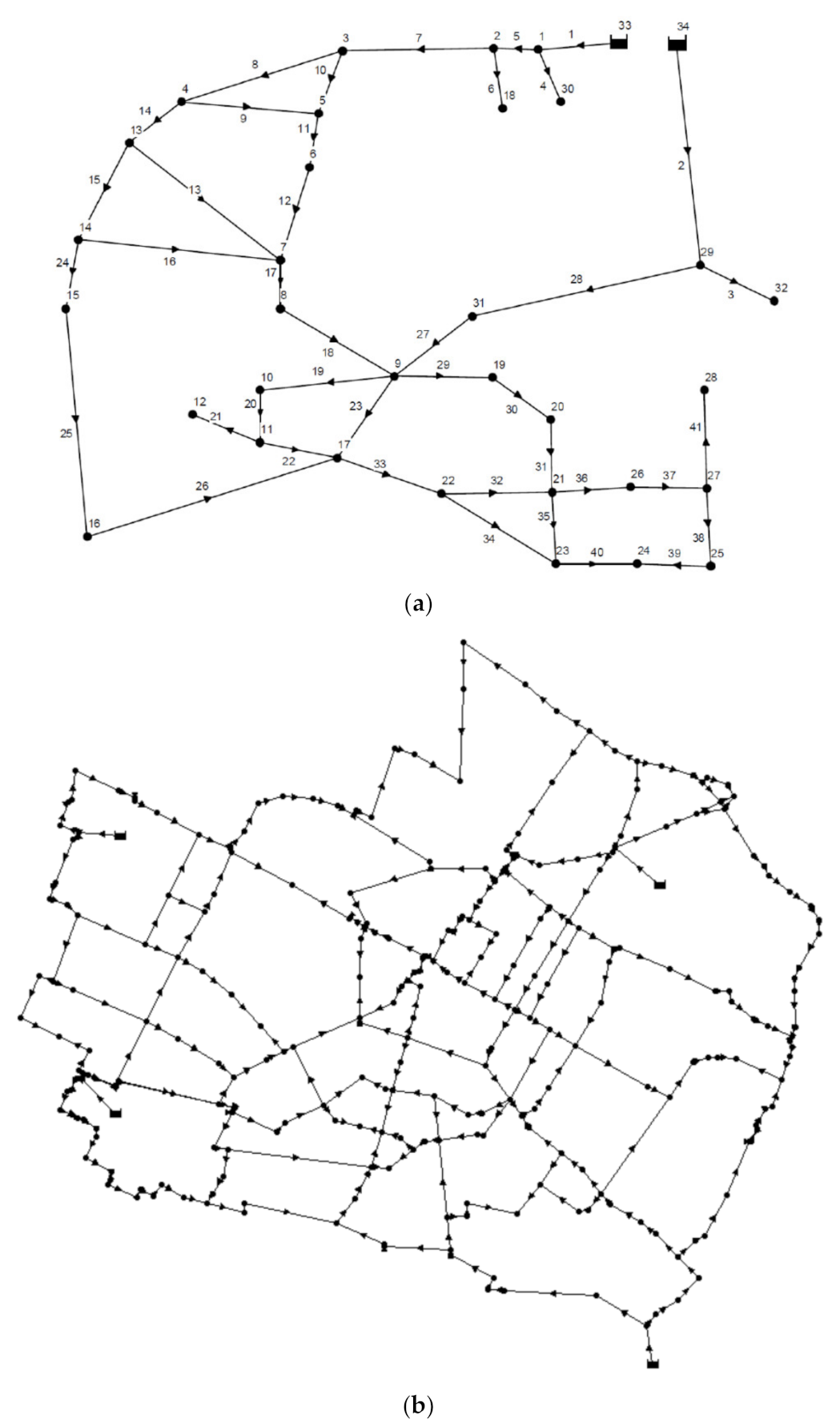
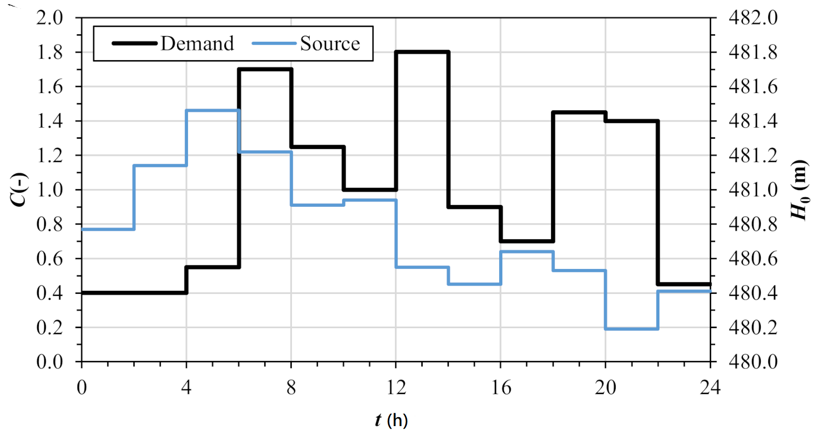
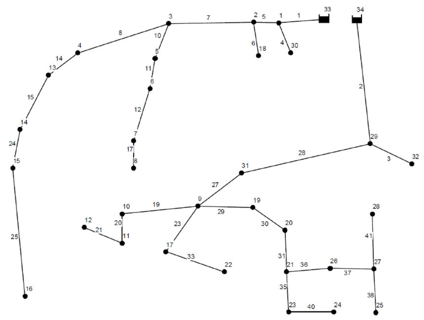
The first case study of this work is the skeletonized WDN serving Santa Maria di Licodia [15,23], a town in Sicily, southern Italy (Figure 1a). This WDN is made up of n = 34 nodes (of which n1 = 32 with unknown head and n0 = 2 source nodes with fixed head, i.e., nodes 33 and 34) and np = 41 pipes. The daily average demand of all WDN users is around 18.5 L/s with nodal demands at demanding nodes ranging from 0.1156 to 1.156 L/s. This WDN features a quite large variability in terms of ground elevations, ranging between 394.8 m above sea level and 465 m above sea level for the demanding nodes. As for leakage, the ratio of daily leakage volume (WL = 1243 m3) to total daily consumption (user consumption + leakage) volume (2841 m3) in the WDN was modelled to be equal to 44%. The main features of the WDN nodes and pipes were derived from the referenced works [15,23]. The daily patterns for the nodal demand multiplicative coefficient C and for the head H0 at the sources are shown in twelve 2 h-long time slots in Figure 2.
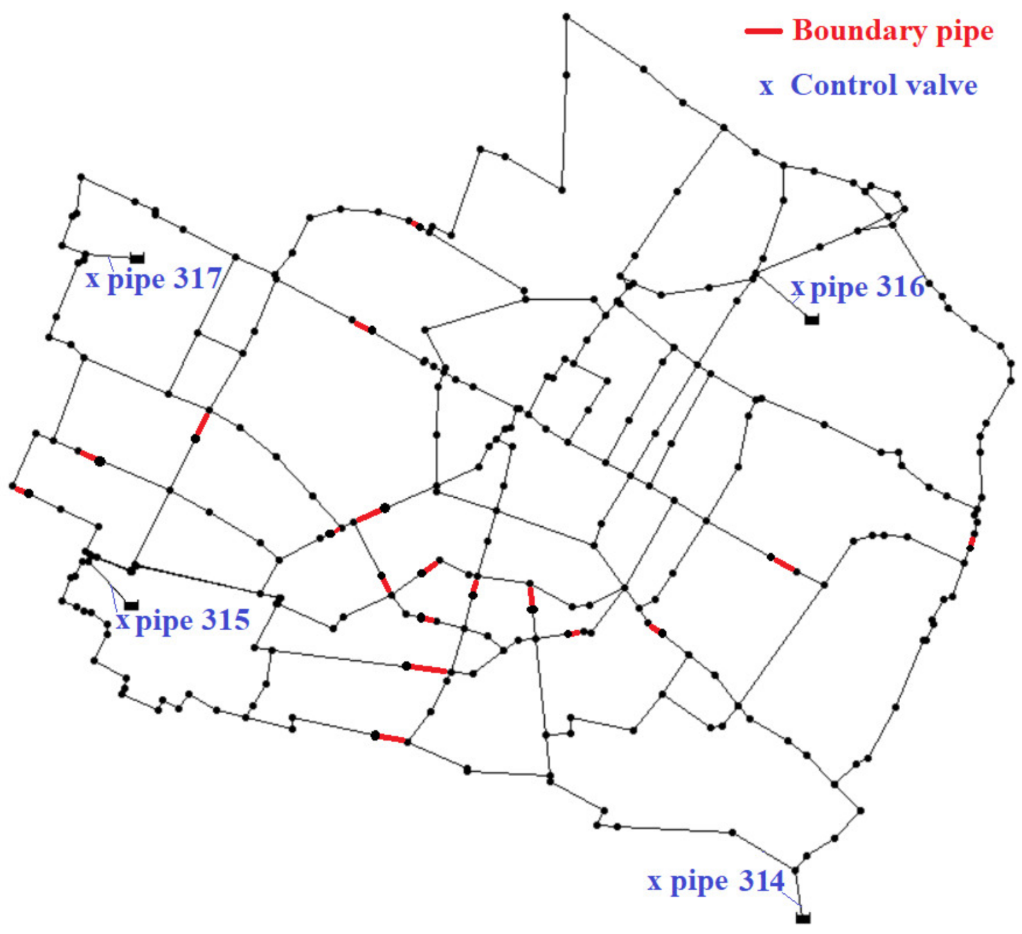
The second case study is the skeletonized WDN of Modena, an Italian city in northern Italy, with n1 = 272 demanding nodes, n0 = 4 sources with fixed head, and np = 317 pipes. In the work of Bragalli et al. [24], the peak demand of about 407 L/s is considered and no pressure-dependent leakage is implemented. In the present work, the yearly average demand was obtained by halving the peak demand. In the context of the average demand, a typical day of operation was considered with three representative time slots, associated with values of the multiplying demand coefficient C equal to 0.7, 1.0, and 1.3, respectively. Nodal emitters were set to obtain a leakage percentage equal to 15%. While this case study has been used in various works [24] for the application of WDN design algorithms, a redundant configuration of diameters in comparison with the minimum cost was considered in the present work, to make this case study feasible partitioning and pressure regulation. The variability in ground elevation at demanding nodes in the second case study, from 30.39 to 74.5 m above sea level, is smaller than in the first case study.
In the applications, after analyzing the pressure conditions in the unpartitioned WDNs, the algorithm based on the sequential addition of control valves was applied. Then, the WDNs were partitioned into a number of partitions equal to the number of the sources, i.e., 2 and 4 partitions for the two case studies, respectively, each of which is fed by a single source. Finally, the sequential addition of control valves was carried out on the partitioned WDN. The results of these applications are reported below.
3.2. Results for the WDN of Santa Maria di Licodia
3.2.1. Analysis of Service Pressure in the Unpartitioned WDN
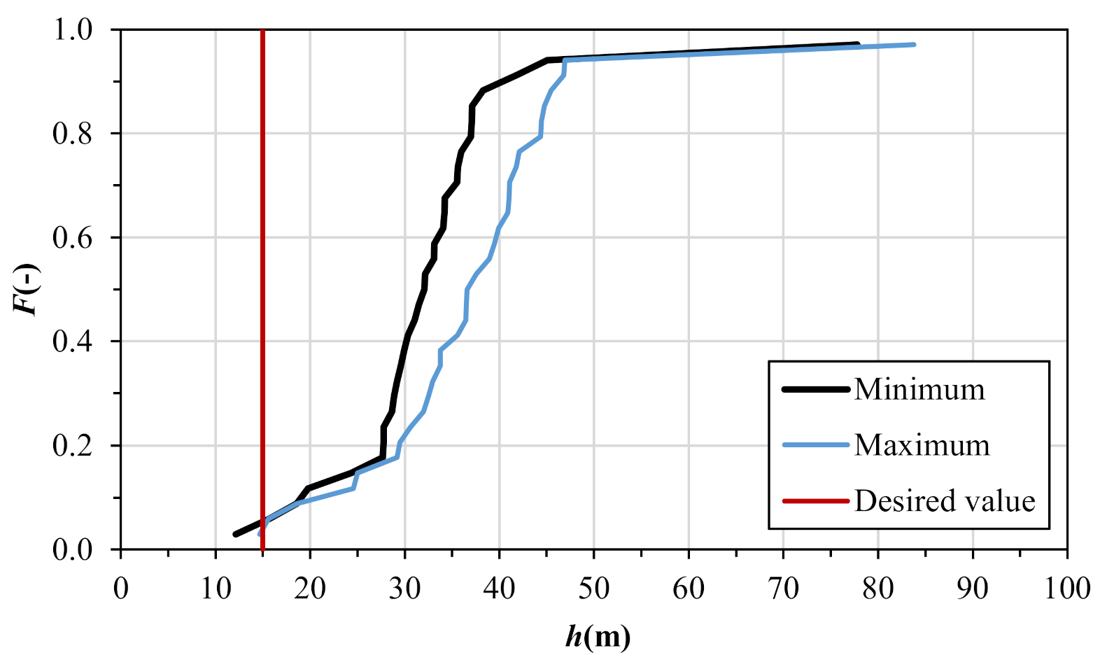
The extended period simulation through a solver based on the pressure-driven extension of EPANET [25,26,27,28] led to daily pressure heads ranging from about 12 to about 45 m for most of the WDN nodes. Due to a much lower ground elevation than its neighbors, node 16 is an outlier, featuring pressure heads in between about 78 and about 84 m. The results of this analysis are summarized in the graph in Figure 3, which reports the cumulated frequency F of the daily maximum and minimum nodal pressure heads.
In a town like Santa Maria di Licodia, in which there are mainly single or double floor households, the minimum desired hdes value for full demand satisfaction can be assumed equal to 15 m. Therefore, as is evident from Figure 3, there is a very large excess of service pressure compared to the desired value hdes for full demand satisfaction.
3.2.2. Application of the Sequential Addition Algorithm to the Unpartitioned WDN
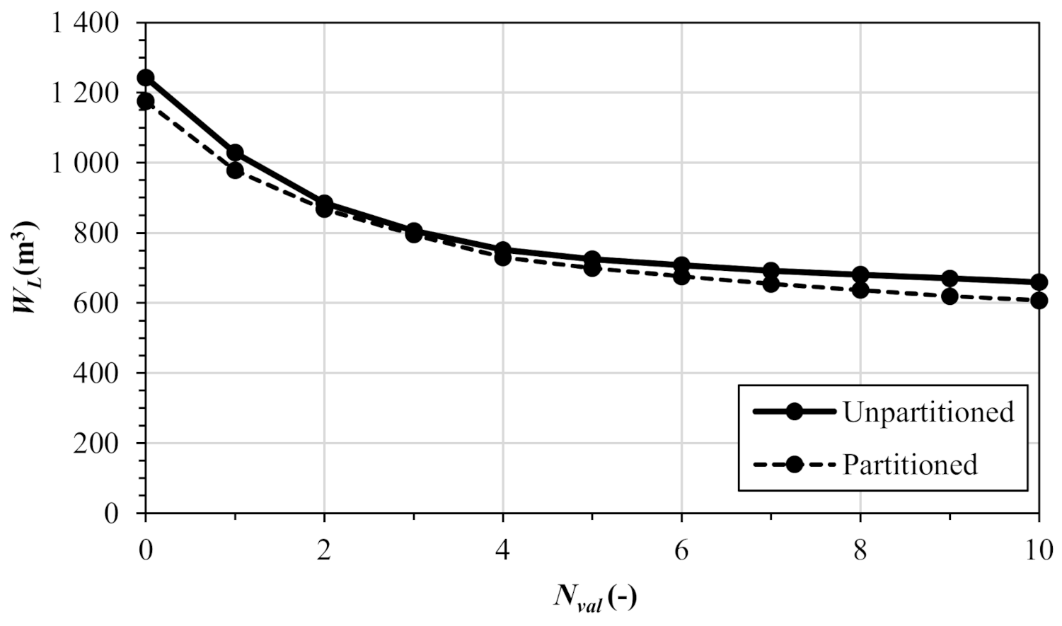
The algorithm for the sequential addition of control valves was applied to the unpartitioned WDN. Taking as benchmark the results in Figure 3, the minimum pressure head constraint considered at the generic demanding node was set at hdes or at the minimum daily pressure head value in the case of pressure excess or deficit, respectively, in comparison with hdes. The results of the sequential addition algorithm up to Nmax = 10 valves are shown in Table 1, showing that significant leakage reductions (by 17%) can be obtained with a single control valve installation in pipe 27. The results improve sensibly up to Nval = 4 valves in pipes 27, 7, 3, and 14, for which the leakage reduction compared to the no-control scenario adds up to about 40%. The Pareto front of optimal solutions in the trade-off between Nval and WL is reported in Figure 4, showing expectedly decreasing values of WL as Nval increases.
3.2.3. WDN Partitioning
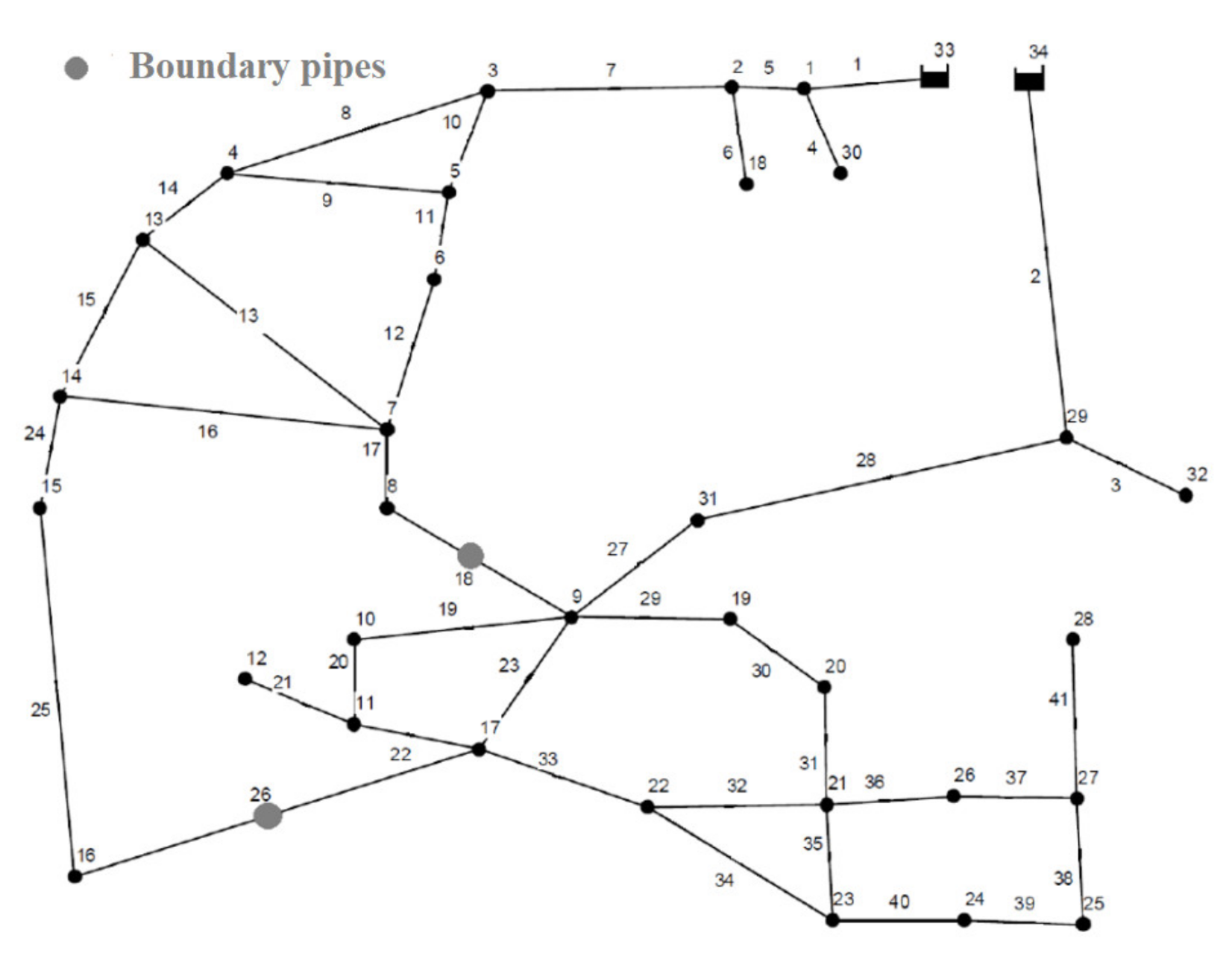
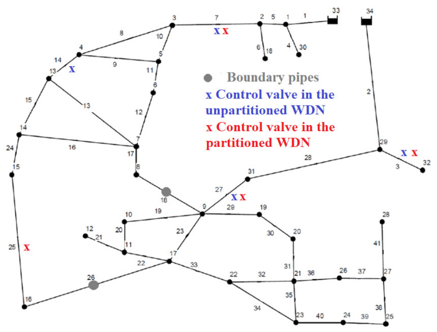
The WDN partitioning algorithm was then applied considering as benchmark the flow directions obtained in the modelling of the WDN (see Figure 1a). Since the WDN features nl = 9 loops, i.e., 8 geometric loops + 1 source interconnection path, the minimization of the transport function led to the removal of 9 pipes, namely, pipes 9, 13, 16, 18, 22, 26, 32, 34, and 39, for opening the loops. As expected, the resulting WDN configuration was a system of two branched networks, each of which was fed by a single source (Figure 5). In fact, the minimization of the transport function enabled clustering the nodes of the WDN into two partitions. To restore a suitable level of reliability in terms of number of closed loops, which help water supply in scenarios of mechanical failure in the WDN, while keeping two separate partitions, all the removed pipes except for pipes 18 and 26 were re-introduced. In fact, pipes 9, 13, 16, 22, 32, 34, and 39 do not contribute to WDN partitioning, while pipes 18 and 26 do. These two pipes were then considered the boundary pipes between the left and right partitions of the WDN (see Figure 6).
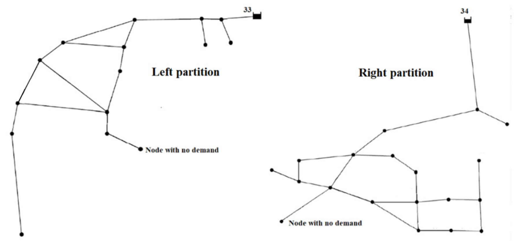
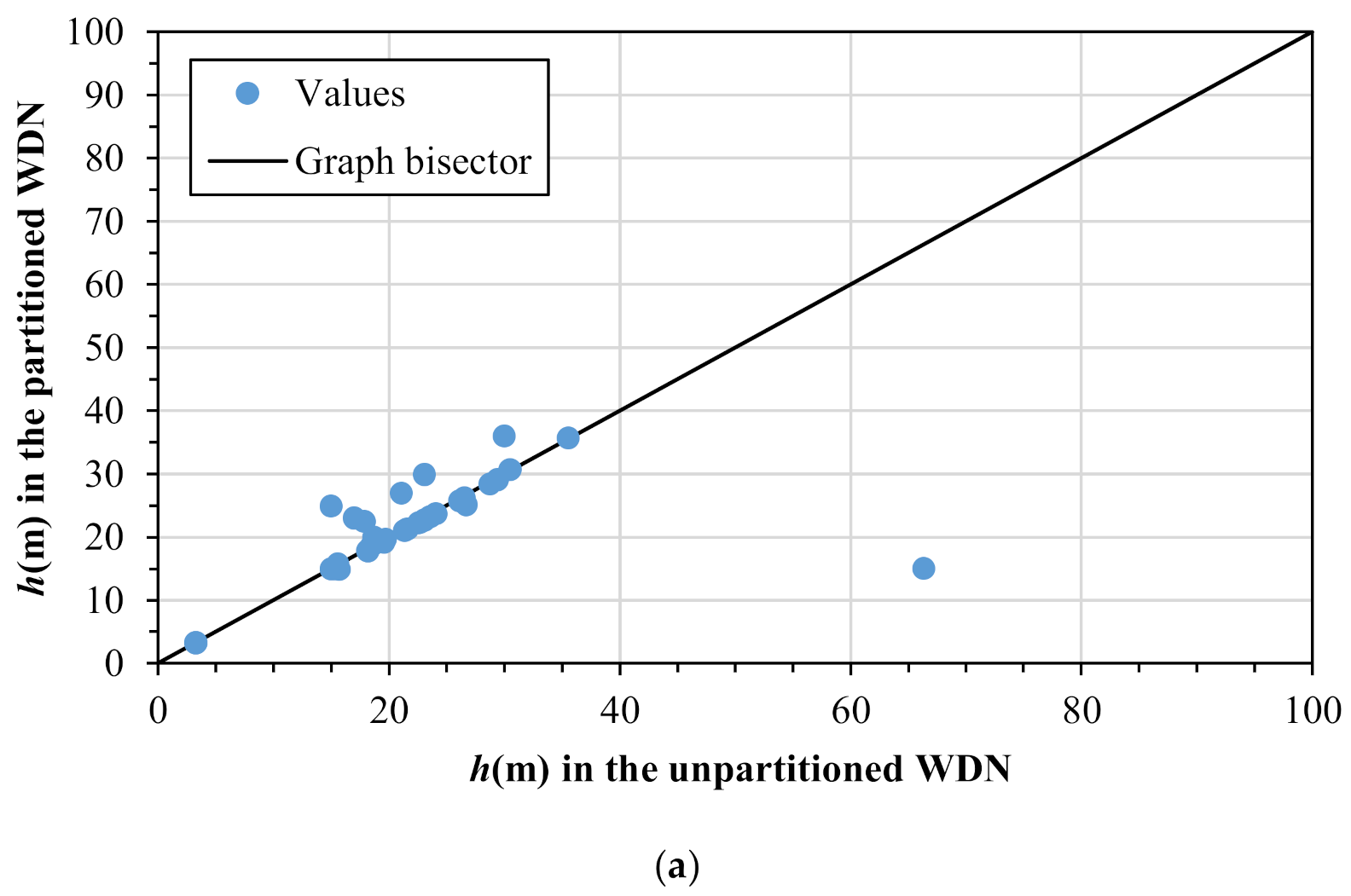
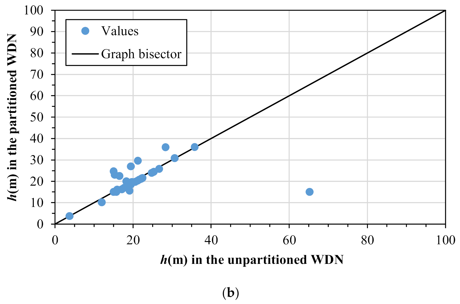
The physical separation of the partitions was verified to be feasible and sustainable in terms of service pressure. The physical separation was obtained by closing the isolation valves in pipe 18 and in pipe 26, in proximity to node 9 and to node 16, respectively, resulting in the WDN configuration with 2 partitions shown in Figure 7. The feasibility check of the partitioning is carried out in Figure 8, showing the comparison of daily maximum (graph a) and minimum (graph b) values between the unpartitioned and partitioned WDN. Globally, this Figure shows that the physical separation of the two partitions causes pressure decreases at some nodes and pressure increases at others. Though the number of nodes with pressure decreases prevails, no inacceptable decreases were observed considering hdes = 15 m, attesting to the feasibility of the physical separation.
By itself, the partitioning of the WDN led to a WL reduction from 1243 to 1176 m3.
3.2.4. Application of the Sequential Addition Algorithm to the Partitioned WDN
The sequential addition algorithm was then applied to the partitioned WDN, leading to the results shown in Table 2. As was expected, the sequential addition yields the lowering of leakage volume from the initial value WL = 1176 m3 also in the partitioned WDN. The valve locations considered in the sequential addition were slightly different from the case of the unpartitioned WDN, due to the flow variations induced by the partitioning. These differences arose starting from the fourth valve installed in the WDN, after the first three valves were installed in pipes 27, 7, and 3 in both cases. While the sequential addition suggested pipe 14 as the location for the fourth valve in the unpartitioned WDN, it suggested pipe 25 after partitioning. In fact, the optimal 4-valve solution obtained in the unpartitioned WDN, including valve locations 27, 7, 3, and 14, yielded a suboptimal leakage volume WL = 780 m3 in the partitioned WDN, in comparison with the solution 27, 7, 3, and 25, which features WL = 730 m3. The choice of pipe 25 instead of pipe 14 as the fourth valve location is motivated as follows. First, the node downstream of pipe 25, i.e., node 16, features very large values of service pressure and leakage, due to its small ground elevation. However, the abatement of service pressure at this node was discouraged in the unpartitioned WDN, since it would have required installation of two control valves, i.e., at pipes 25 and 26, respectively. Therefore, the sequential addition algorithm preferred to choose another location for the fourth valve in the unpartitioned WDN. In the case of the partitioned WDN, instead, the disconnection of pipe 26 from node 16 due to the partitioning made pipe 25 branched, and, therefore, a suitable site for control valve installation and pressure regulation.
The number Nval of control valves being equal, the partitioning was observed to yield benefits in terms of WL reduction. These benefits were estimated to be ranging from about 1% to about 8% (last column in Table 2). This is the result of the lower service pressure existing in the partitioned WDN, starting from the initial scenario with no control valves installed.
The comparison in terms of Pareto front Nval-WL between unpartitioned and partitioned WDN is shown in Figure 4, highlighting lower values of WL in the partitioned WDN for each value of Nval.
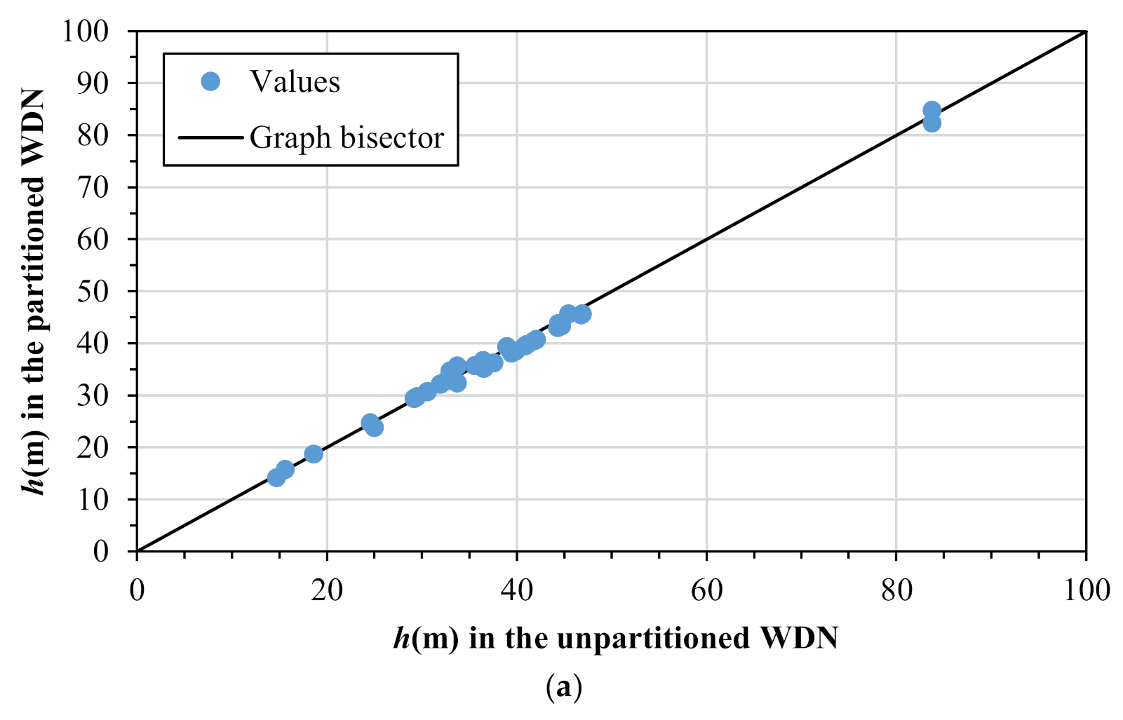
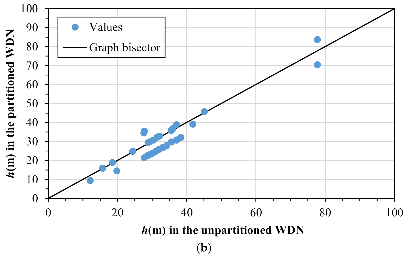
The following Figure 9 reports the comparison of daily maximum and minimum pressure heads h (m) between the unpartitioned and partitioned WDN, in the case of four control valves (locations 27, 7, 3, and 14 and locations 27, 7, 3, and 25 for the unpartitioned and partitioned WDN, respectively, see Figure 10).
The four-valve scenario was chosen because it lies on the knee of the Pareto front Nval-WL for both the unpartitioned and partitioned WDNs (Figure 4). This attests to the fact that, up to Nval = 4, the addition of a control valve is effectively paid back in terms of leakage reduction. For both the unpartitioned and partitioned WDNs, the valve settings expressed in terms of pressure head at the downstream node are quite constant in the day and very close to hdes = 15 m, due to the altimetry of the urban center. Most nodes in the unpartitioned WDN have slightly lower pressure heads than those in the partitioned WDN. The only evident exception is the situation of node 16, for which a large difference exists between the pressure head in the unpartitioned WDN (around 65 m) and in the partitioned WDN (around 15 m). This is the result of what was highlighted about the optimal addition of the fourth control valve in unpartitioned and partitioned WDN. However, this significant difference of service pressure at node 16 enables lower daily leakage volume to be obtained for the partitioned WDN (730 vs. 751 m3). Overall, as expected, lower pressure heads are observed in the presence of four control valves than in the absence of control valves (compare Figure 9 with Figure 8).
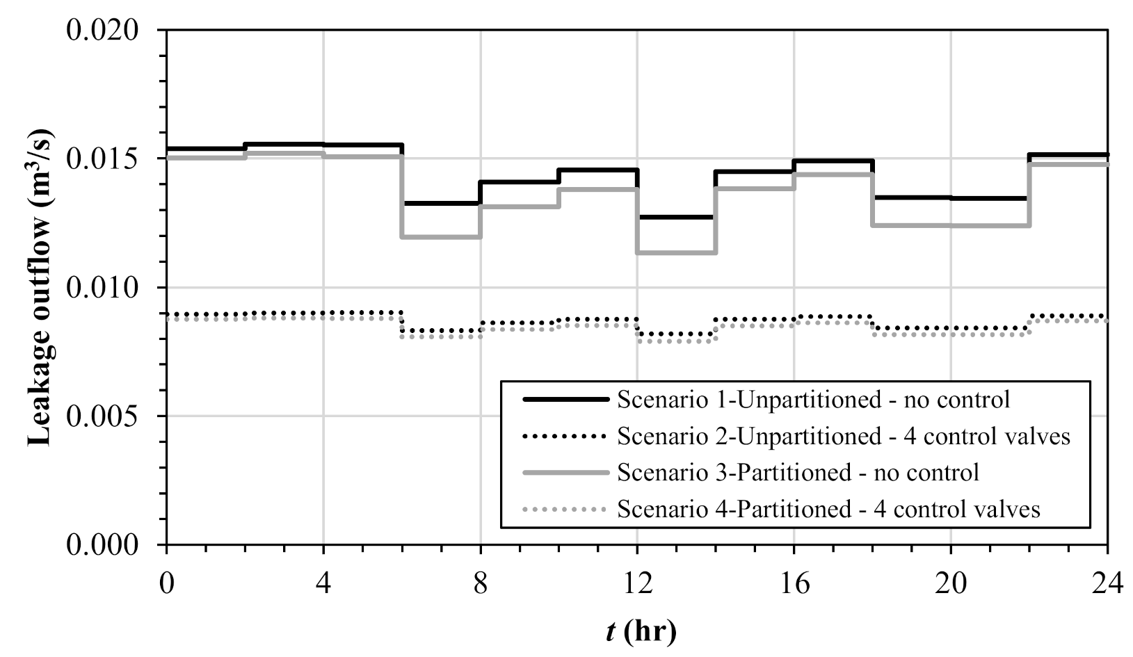
A last analysis was carried out concerning the daily pattern of the total leakage outflow, which is a result of the service pressure in the WDN. For this analysis, four scenarios were selected, namely the unpartitioned WDN in the absence of control valves (scenario 1); the unpartitioned WDN with four optimal valves installed at pipes 27, 7, 3, and 14, respectively (scenario 2); the partitioned WDN in the absence of control valves (scenario 3); and the partitioned WDN with four optimal control valves installed (scenario 4) at pipes 27, 7, 3, and 25. As the following Figure 11 shows, this pattern features sensible fluctuations around the average value of about 0.0144 m3/s in scenario 1, with overshooting and undershooting present mainly at nighttime and daytime, respectively. The partitioning causes the lowering of the pattern to the average value of 0.0136 m3/s (compare scenario 3 with scenario 1). The distance of the pattern in scenario 3 from the pattern in scenario 1 is larger at daytime than at nighttime. In the scenarios with control valves, i.e., scenarios 2 and 4, the patterns are much flatter than in the no control scenarios 1 and 3. In fact, they feature very small fluctuations around their average values of 0.0087 and 0.0084 m3/s, respectively, resulting from poorly variable service pressure conditions in the day.
3.3. Results for the WDN of Modena
3.3.1. Analysis of Service Pressure in the Unpartitioned WDN
The extended period simulation through a solver based on the pressure-driven extension of EPANET [25,26,27,28] led to daily pressure heads ranging from about 28 to about 40 m for all the WDN nodes. The results of this analysis are summarized in the graph in Figure 12, which reports the cumulated frequency F of the daily maximum and minimum nodal pressure heads.
In this case study, the minimum desired hdes value for full demand satisfaction is assumed equal to 20 m. Therefore, as is evident from Figure 12, there is a very large excess of service pressure compared to the desired value hdes for full demand satisfaction.
3.3.2. Application of the Sequential Addition Algorithm to the Unpartitioned WDN
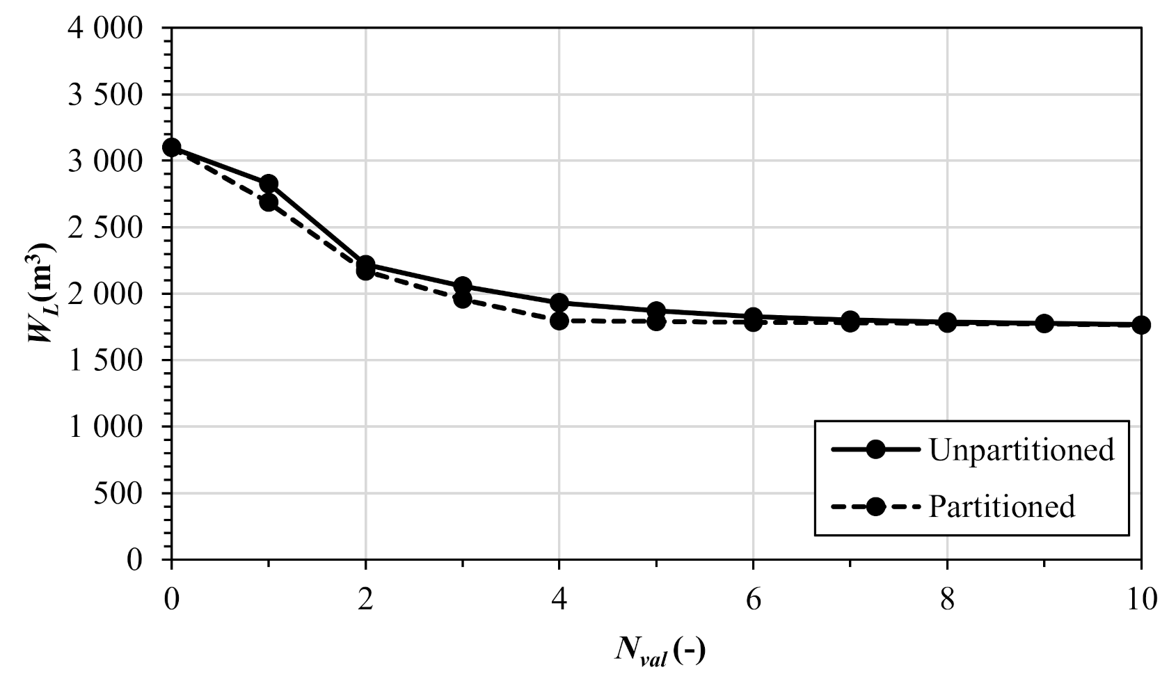
The algorithm for the sequential addition of control valves was applied to the unpartitioned WDN, taking hdes = 20 m as the minimum pressure head constraint at the generic demanding node. The Pareto front of optimal solutions obtained in the trade-off between Nval and WL is reported in Figure 13, showing expectedly decreasing values of WL as Nval increases. Like for the first case study, the decrease is significant up to Nval = 4, for which a reduction in WL by about 38% is observed in comparison with the no control scenario.
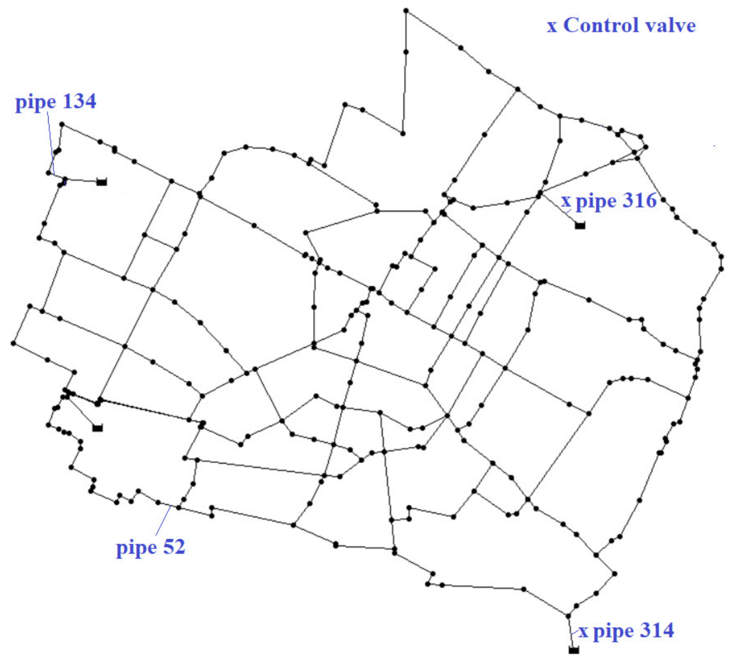
As an example, Figure 14 shows the optimal location of the control valves at pipes 52, 134, 314, and 316, quite close to the exit of the four sources.
3.3.3. WDN Partitioning
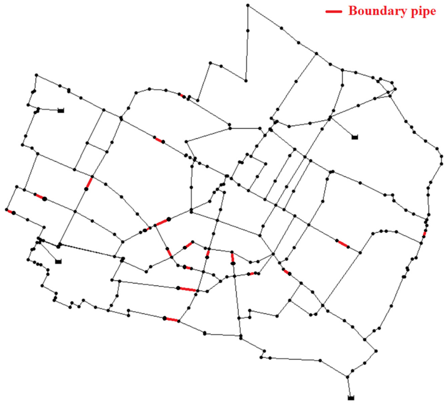
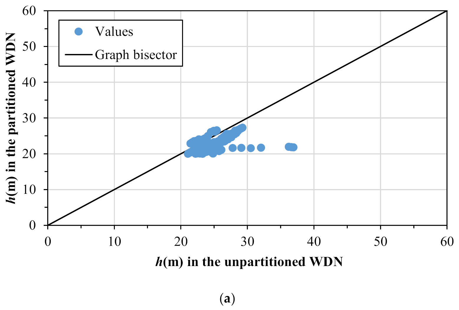
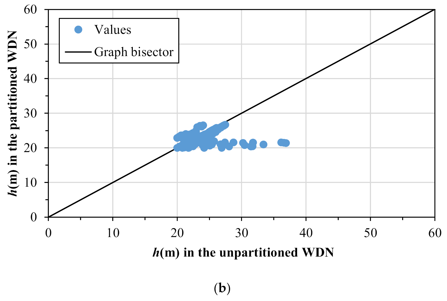
The WDN partitioning algorithm was then applied considering as benchmark the flow directions obtained in the modelling of the WDN (see Figure 1b). Since the WDN features nl = 49 loops, i.e., 46 geometric loops + 3 source interconnection paths, the minimization of the transport function led to the removal of 49 pipes, resulting in a system of 4 branched partitions each of which fed by a single source. To restore a suitable level of reliability in terms of loops while keeping four separate partitions, 31 of the removed pipes were re-introduced. The other 18 pipes were then considered the boundary pipes between the partitions of the WDN (see Figure 15). Like in the first case study, the physical separation of the partitions was verified to be feasible and sustainable in terms of service pressure. The physical separation was obtained by closing the isolation valves at one end of each pipe. The feasibility check of the partitioning is carried out in Figure 16, showing the comparison of pressure head values between the unpartitioned and partitioned WDN. Globally, this Figure shows that the physical separation of the four partitions causes pressure decreases at some nodes and pressure increases at others. Though the number of nodes with pressure decreases prevails, no inacceptable decreases were observed considering hdes = 20 m, attesting to the feasibility of the physical separation.
By itself, the partitioning of the WDN led to a slight WL reduction from 3101 to 3100 m3.
3.3.4. Application of the Sequential Addition Algorithm to the Partitioned WDN
The sequential addition algorithm was then applied to the partitioned WDN. The Pareto front WL(Nval) is shown in the graph in Figure 13 in comparison with the front obtained in the unpartitioned WDN. Like in the first case study, all the dots of the Pareto front of the partitioned WDN are slightly below those of the unpartitioned WDN, highlighting lower leakage volumes by up to about 7%, the number of installed control valves being the same. To have better insight into this aspect, the optimal location of four control valves in the partitioned WDN can be analyzed (see Figure 17) and compared with the four-valve scenario in the unpartitioned WDN (Figure 14). As Figure 14 and Figure 17 show, the valve locations obtained in the case of the partitioned WDN (pipes 314, 315, 316, and 317) are different from the case of the unpartitioned WDN, due to the flow variations induced by the partitioning, though being all close to the WDN sources. Furthermore, the downstream pressure settings at the control valves are equal to 22.93, 22.50, 25.04, and 21.58 m, with an average value of 23.01 m. The settings are smaller than those equal to 25.72, 29.28, 23.13 and 25.72 m (average value of 25.97 m), obtained for the control valves installed in pipes 52, 134, 314, and 316, respectively, in the unpartitioned WDN. This proves that the partitioning improves regulation of service pressure in the WDN. Therefore, leakage volume is lower in the partitioned WDN (WL= 1796.61 m3) than the unpartitioned WDN (WL= 1931.91 m3). The lower leakage volume is consistent with the results in Figure 18, globally pointing out lower pressure heads for the partitioned WDN.
A last analysis concerns the pattern of leakage outflows from the WDN in the three time slots in the four scenarios analyzed, i.e., unpartitioned WDN—no control, unpartitioned WDN—4 valves, partitioned WDN—no control, and partitioned WDN—4 valves. As Table 3 shows, similarly to the first case study, the installation of control valves reduces the variability of leakage outflow rates during the day, in both the unpartitioned and partitioned WDN.
4. Discussion
In this work, the combined effects of WDN partitioning and optimal location of control valves for leakage reduction were evaluated on the skeletonized model of the WDN serving two Italian urban centers. The partitioning and the optimal location of control valves were carried out using a methodology based on the minimization of the transport function and an algorithm based on the sequential addition of valves, respectively. The analysis was carried out based on the following sequence of steps:
- Analysis of service pressure in the unpartitioned WDN.
- Optimal location of control valves in the unpartitioned WDN.
- WDN partitioning in the absence of control valves.
- Optimal location of control valves in the partitioned WDN.
The main findings of the work are the following:
- When involving physical separation between partitions, WDN partitioning can result per se in the slight lowering in service pressure and, therefore, in leakage attenuation.
- Due to variations in flow distribution, the valve locations optimally selected in a partitioned WDN may differ from those in the unpartitioned WDN.
- The number of optimally installed being the same, the partitioned WDN enables achievement of better leakage reduction performance than the unpartitioned WDN.
- In both the unpartitioned and partitioned WDNs, the installation of control valves makes the daily pattern of leakage outflows flatter, by reducing the variability of service pressure in the day.
Overall, the results of this work proved that the partitioning performed based on the minimization of the transport function helps in improving the effectiveness of control valves in reducing service pressure and leakage. However, different results could be obtained applying other partitioning algorithms to other case studies. Future work will be dedicated to the comparison of various WDN partitioning algorithms present in the scientific literature, to analyze the extent to which the change in partitioning algorithm may impact on the optimal location of control valves. This will enable identification of the partitioning algorithm that performs best in combination with algorithms for optimal valve installation/regulation.
Author Contributions
Conceptualization, E.C. and G.P.; methodology, E.C. and G.P.; investigation, D.C.; writing—original draft preparation, E.C.; writing—review and editing, G.P. All authors have read and agreed to the published version of the manuscript.
Funding
This research received no external funding.
Institutional Review Board Statement
Not applicable.
Informed Consent Statement
Not applicable.
Data Availability Statement
The data necessary for the calculations are all reported in the paper.
Acknowledgments
This work was done using funds and resources available from the Universities of Catania and Pavia.
Conflicts of Interest
The authors declare no conflict of interest.
References
- Farley, M.; Trow, S. Losses in Water Distribution Networks; IWA: London, UK, 2003. [Google Scholar]
- Vicente, D.; Garrote, L.; Sánchez, R.; Santillán, D. Pressure Management in Water Distribution Systems: Current Status, Proposals, and Future Trends. J. Water Resour. Plan. Manag. 2016, 142, 04015061. [Google Scholar] [CrossRef]
- Creaco, E.; Campisano, A.; Fontana, N.; Marini, G.; Page, P.R.; Walski, T. Real time control of water distribution networks: A state-of-the-art review. Water Res. 2019, 161, 517–530. [Google Scholar] [CrossRef] [PubMed]
- Jowitt, P.W.; Xu, C. Optimal Valve Control in Water-Distribution Networks. J. Water Resour. Plan. Manag. 1990, 116, 455–472. [Google Scholar] [CrossRef]
- Vairavamoorthy, K.; Lumbers, J. Leakage reduction in water distribution systems: Optimal valve control. J. Hydraul. Eng. 1998, 124, 1146–1154. [Google Scholar] [CrossRef]
- Reis, L.; Porto, R.; Chaudhry, F. Optimal location of control valves in pipe networks by genetic algorithm. J. Water Resour. Plan. Manag. 1997, 123, 317–326. [Google Scholar] [CrossRef]
- Araujo, L.; Ramos, H.; Coelho, S. Pressure control for leakage minimisation in water distribution systems management. Water Resour. Manag. 2006, 20, 133–149. [Google Scholar] [CrossRef]
- Covelli, C.; Cozzolino, L.; Cimorrelli, L.; Della Morte, R.; Pianese, D. Optimal Location and Setting of PRVs in WDS for Leakage Minimization. Water Resour. Manag. 2016, 30, 1803–1817. [Google Scholar] [CrossRef] [Green Version]
- Ali, M.E. Knowledge-Based Optimization Model for Control Valve Locations in Water Distribution Networks. J. Water Resour. Plan. Manag. 2015, 141, 04014048. [Google Scholar] [CrossRef]
- Liberatore, S.; Sechi, G.M. Location and Calibration of Valves in Water Distribution Networks Using a Scatter-Search Meta-heuristic Approach. Water Resour. Manag. 2009, 23, 1479–1495. [Google Scholar] [CrossRef]
- De Paola, F.; Galdiero, E.; Giugni, M. Location and Setting of Valves in Water Distribution Networks Using a Harmony Search Approach. J. Water Resour. Plan. Manag. 2017, 143, 04017015. [Google Scholar] [CrossRef]
- Nicolini, M.; Zovatto, L. Optimal Location and Control of Pressure Reducing Valves in Water Networks. J. Water Resour. Plan. Manag. 2009, 135, 178–187. [Google Scholar] [CrossRef]
- Pezzinga, G.; Gueli, R. Discussion of “Optimal Location of Control Valves in Pipe Networks by Genetic Algorithm”. J. Water Resour. Plan. Manag. 1999, 125, 65–67. [Google Scholar] [CrossRef]
- Creaco, E.; Pezzinga, G. Multi-objective optimization of pipe replacements and control valve installations for leakage attenuation in water distribution networks. J. Water Resour. Plan. Manag. 2015, 141, 04014059. [Google Scholar] [CrossRef]
- Creaco, E.; Pezzinga, G. Embedding Linear Programming in Multi Objective Genetic Algorithms for Reducing the Size of the Search Space with Application to Leakage Minimization in Water Distribution Networks. Environ. Model. Softw. 2015, 69, 308–318. [Google Scholar] [CrossRef]
- Creaco, E.; Pezzinga, G. Comparison of Algorithms for the Optimal Location of Control Valves for Leakage Reduction in WDNs. Water 2018, 10, 466. [Google Scholar] [CrossRef] [Green Version]
- UK Water Industry Research Limited. A Manual of DMA Practice; Water Industry Research: London, UK, 1999. [Google Scholar]
- Bui, X.K.; Marlim, M.S.; Kang, D. Water Network Partitioning into District Metered Areas: A State-Of-The-Art Review. Water 2020, 12, 1002. [Google Scholar] [CrossRef] [Green Version]
- Ciaponi, C.; Creaco, E.; Franchioli, L.; Papiri, S. The importance of the minimum path criterion in the design of water distribution networks. Water Sci. Technol. Water Supply 2017, 17, 1558–1567. [Google Scholar] [CrossRef]
- Stephenson, D. Pipeflow Analysis; Elsevier: Amsterdam, The Netherlands; New York, NY, USA, 1984. [Google Scholar]
- Dantzig, G.B. Linear Programming and Extensions; Princeton U P: Princeton, NJ, USA, 1963. [Google Scholar]
- Scarpa, F.; Lobba, A.; Becciu, G. Elementary DMA Design of Looped Water Distribution Networks with Multiple Sources. J. Water Resour. Plan. Manag. 2016, 142, 04016011. [Google Scholar] [CrossRef] [Green Version]
- Pezzinga, G. Procedure per la riduzione delle perdite mediante il controllo delle pressioni. In Ricerca e Controllo Delle Perdite Nelle reti di Condotte. Manuale per una Moderna Gestione Degli Acquedotti; Brunone, B., Ferrante, M., Meniconi, S., Eds.; Città Studi Edizioni: Novara, Italy, 2008. [Google Scholar]
- Bragalli, C.; D’Ambrosio, C.; Lee, J.; Lodi, A.; Toth, P. On the optimal design of water distribution networks: A practical MINLP approach. Optim. Eng. 2012, 13, 219–246. [Google Scholar] [CrossRef]
- Ciaponi, C.; Creaco, E. Comparison of Pressure-Driven Formulations for WDN Simulation. Water 2018, 10, 523. [Google Scholar] [CrossRef] [Green Version]
- Cheung, P.B.; Van Zyl, E.; Reis, L.F.R. Extension of EPANET for pressure driven demand modelling in water distribution system. In Proceedings of the Eighth International Conference on Computing and Control for the Water Industry; University of Exeter: Exeter, UK, 2005; ISBN 0-9539140-2-X. [Google Scholar]
- Morley, M.S.; Tricarico, C. Pressure Driven Demand Extension for EPANET (EPANETpdd). Technical Report 2008/02: (Revised 26/03/2014). University of Exeter. Available online: http://hdl.handle.net/10871/14721 (accessed on 5 April 2021).
- Boryczko, K.; Tchorzewska-Cieslak, A. Analysis and assessment of the risk of lack of water supply using the EPANET program. In Environmental Engineering IV; Pawlowski, D., Ed.; Taylor & Francis Group: London, UK, 2013; pp. 63–68. [Google Scholar]
Figure 1.
Water distribution networks (WDNs) of (a) Santa Maria di Licodia and (b) Modena. Arrows indicate flow direction after the preliminary analysis.
Figure 1.
Water distribution networks (WDNs) of (a) Santa Maria di Licodia and (b) Modena. Arrows indicate flow direction after the preliminary analysis.

Figure 2.
WDN of Santa Maria di Licodia. Daily patterns of demand multiplicative coefficient C and head H0 at sources.
Figure 2.
WDN of Santa Maria di Licodia. Daily patterns of demand multiplicative coefficient C and head H0 at sources.

Figure 3.
WDN of Santa Maria di Licodia. Cumulative frequency F(−) of maximum and minimum daily pressure heads h (m), in comparison with the minimum desired value hdes.
Figure 3.
WDN of Santa Maria di Licodia. Cumulative frequency F(−) of maximum and minimum daily pressure heads h (m), in comparison with the minimum desired value hdes.

Figure 4.
WDN of Santa Maria di Licodia. Pareto fronts of optimal solution in the trade-off between Nval and WL.
Figure 4.
WDN of Santa Maria di Licodia. Pareto fronts of optimal solution in the trade-off between Nval and WL.

Figure 5.
WDN of Santa Maria di Licodia. WDN with loops opened based on the results of the optimization.
Figure 5.
WDN of Santa Maria di Licodia. WDN with loops opened based on the results of the optimization.

Figure 6.
WDN of Santa Maria di Licodia. Identification of the boundary pipes for the partitioning.

Figure 7.
WDN of Santa Maria di Licodia. Partitioning of the WDN into two partitions.

Figure 8.
WDN of Santa Maria di Licodia. In the absence of control valves, comparison of daily maximum (a) and minimum (b) pressure heads h (m) between the unpartitioned and partitioned WDN.
Figure 8.
WDN of Santa Maria di Licodia. In the absence of control valves, comparison of daily maximum (a) and minimum (b) pressure heads h (m) between the unpartitioned and partitioned WDN.


Figure 9.
WDN of Santa Maria di Licodia. In the case of four control valves, comparison of daily maximum (a) and minimum (b) pressure heads h (m) between the unpartitioned and partitioned WDN.
Figure 9.
WDN of Santa Maria di Licodia. In the case of four control valves, comparison of daily maximum (a) and minimum (b) pressure heads h (m) between the unpartitioned and partitioned WDN.


Figure 10.
WDN of Santa Maria di Licodia. Location of control valves in the unpartitioned and partitioned WDNs.
Figure 10.
WDN of Santa Maria di Licodia. Location of control valves in the unpartitioned and partitioned WDNs.

Figure 11.
WDN of Santa Maria di Licodia. Daily pattern of leakage outflows in no control and control scenarios, for both the unpartitioned and partitioned WDN.
Figure 11.
WDN of Santa Maria di Licodia. Daily pattern of leakage outflows in no control and control scenarios, for both the unpartitioned and partitioned WDN.

Figure 12.
WDN of Modena. Cumulative frequency F(−) of daily maximum and minimum pressure heads h (m), in comparison with the minimum desired value hdes.
Figure 12.
WDN of Modena. Cumulative frequency F(−) of daily maximum and minimum pressure heads h (m), in comparison with the minimum desired value hdes.

Figure 13.
WDN of Modena. Pareto fronts of optimal solution in the trade-off between Nval and WL.

Figure 14.
WDN of Modena. In the case of four control valves, positions of the valves in the unpartitioned WDN.
Figure 14.
WDN of Modena. In the case of four control valves, positions of the valves in the unpartitioned WDN.

Figure 15.
WDN of Modena. Positions of the boundary pipes in WDN partitioning.

Figure 16.
WDN of Modena. In the absence of control valves, comparison of daily maximum (a) and minimum (b) pressure heads h (m) between the unpartitioned and partitioned WDN.
Figure 16.
WDN of Modena. In the absence of control valves, comparison of daily maximum (a) and minimum (b) pressure heads h (m) between the unpartitioned and partitioned WDN.

Figure 17.
WDN of Modena. Positions of the control valves in the partitioned WDN.

Figure 18.
WDN of Modena. In the presence of four control valves, comparison of daily maximum (a) and minimum (b) pressure heads h (m) between the unpartitioned and partitioned WDN.
Figure 18.
WDN of Modena. In the presence of four control valves, comparison of daily maximum (a) and minimum (b) pressure heads h (m) between the unpartitioned and partitioned WDN.


Table 1.
Water distribution network (WDN) of Santa Maria di Licodia. Results of the sequential addition of control valves in the unpartitioned WDN. Locations and leakage volumes.
Table 1.
Water distribution network (WDN) of Santa Maria di Licodia. Results of the sequential addition of control valves in the unpartitioned WDN. Locations and leakage volumes.
| Nval | Valve Locations on Unpartitioned WDN | WL (m3) on Unpartitioned WDN |
|---|---|---|
| 0 | – | 1243 |
| 1 | 27 | 1029 |
| 2 | 27, 7 | 885 |
| 3 | 27, 7, 3 | 805 |
| 4 | 27, 7, 3, 14 | 751 |
| 5 | 27, 7, 3, 14, 33 | 725 |
| 6 | 27, 7, 3, 14, 33, 4 | 708 |
| 7 | 27, 7, 3, 14, 33, 4, 2 | 692 |
| 8 | 27, 7, 3, 14, 33, 4, 2, 41 | 680 |
| 9 | 27, 7, 3, 14, 33, 4, 2, 41, 6 | 670 |
| 10 | 27, 7, 3, 14, 33, 4, 2, 41, 6, 30 | 659 |
Table 2.
WDN of Santa Maria di Licodia. Results of the sequential addition of control valves in the partitioned WDN. Locations, leakage volumes, and benefits of the partitioning.
Table 2.
WDN of Santa Maria di Licodia. Results of the sequential addition of control valves in the partitioned WDN. Locations, leakage volumes, and benefits of the partitioning.
| Nval | Valve Locations on Partitioned WDN | WL (m3) on Partitioned WDN | WL (m3) on Unpartitioned WDN | Benefits (%) of Partitioning |
|---|---|---|---|---|
| 0 | - | 1176 | 1243 | 5.42 |
| 1 | 27 | 978 | 1029 | 4.94 |
| 2 | 27, 7 | 867 | 885 | 2.00 |
| 3 | 27, 7, 3 | 795 | 805 | 1.24 |
| 4 | 27, 7, 3, 25 | 730 | 751 | 2.82 |
| 5 | 27, 7, 3, 25, 26 | 699 | 725 | 3.54 |
| 6 | 27, 7, 3, 25, 26, 2 | 676 | 708 | 4.56 |
| 7 | 27, 7, 3, 25, 26, 2, 33 | 654 | 692 | 5.45 |
| 8 | 27, 7, 3, 25, 26, 2, 33, 4 | 637 | 680 | 6.37 |
| 9 | 27, 7, 3, 25, 26, 2, 33, 24 | 619 | 670 | 7.58 |
| 10 | 27, 7, 3, 25, 26, 2, 33, 24, 17 | 607 | 659 | 7.85 |
Table 3.
WDN of Modena. Leakage outflow rates (m3/s) in the three time slots of the day in different scenarios.
Table 3.
WDN of Modena. Leakage outflow rates (m3/s) in the three time slots of the day in different scenarios.
| Time Slot | Scenario 1 Unpartitioned WDN, no Control | Scenario 2 Unpartitioned WDN, 4 Valves | Scenario 3 Partitioned WDN, no Control | Scenario 4 Partitioned WDN, 4 Valves |
|---|---|---|---|---|
| 1 | 0.0363 | 0.0233 | 0.0365 | 0.0207 |
| 2 | 0.0359 | 0.0218 | 0.0359 | 0.0208 |
| 3 | 0.0354 | 0.0220 | 0.0352 | 0.0209 |
Publisher’s Note: MDPI stays neutral with regard to jurisdictional claims in published maps and institutional affiliations. |
© 2021 by the authors. Licensee MDPI, Basel, Switzerland. This article is an open access article distributed under the terms and conditions of the Creative Commons Attribution (CC BY) license (https://creativecommons.org/licenses/by/4.0/).
Share and Cite
MDPI and ACS Style
Creaco, E.; Castagnolo, D.; Pezzinga, G. Assessing the Impact of Partitioning on Optimal Installation of Control Valves for Leakage Minimization in WDNs. Water 2021, 13, 1003. https://doi.org/10.3390/w13071003
AMA Style
Creaco E, Castagnolo D, Pezzinga G. Assessing the Impact of Partitioning on Optimal Installation of Control Valves for Leakage Minimization in WDNs. Water. 2021; 13(7):1003. https://doi.org/10.3390/w13071003
Chicago/Turabian StyleCreaco, Enrico, Dario Castagnolo, and Giuseppe Pezzinga. 2021. "Assessing the Impact of Partitioning on Optimal Installation of Control Valves for Leakage Minimization in WDNs" Water 13, no. 7: 1003. https://doi.org/10.3390/w13071003
Note that from the first issue of 2016, this journal uses article numbers instead of page numbers. See further details here.