
Setting Priorities in River Management Using Habitat Suitability Models


1
Aquatic Ecology Research Unit, Department of Animal Sciences and Aquatic Ecology, Ghent University, 9000 Ghent, Belgium
2
Fluves, 9000 Ghent, Belgium
3
Flanders Marine Institute, 8400 Ostend, Belgium
*
Author to whom correspondence should be addressed.
Water 2021, 13(7), 886; https://doi.org/10.3390/w13070886
Submission received: 25 January 2021
/
Revised: 19 March 2021
/
Accepted: 22 March 2021
/
Published: 24 March 2021
(This article belongs to the Special Issue Assessment of Species Community Structure and Ecological Water Quality)
Abstract
:Worldwide river systems are under pressure from human development. River managers need to identify the most important stressors in a stream basin, to propose effective management interventions for river restoration. In the European Union, the Water Framework Directive proposes the ecological status as the management endpoint for these interventions. Many decision support tools exist that use predictive water quality models to evaluate different river management scenarios, but only a few consider a river’s ecological status in this analysis explicitly. This paper presents a novel method, which combines abiotic monitoring data and biological monitoring data, to provide information and insight on why the ecological status does not reach the good status. We use habitat suitability models as a decision support tool, which can identify the most important stressors in river systems to define management scenarios. To this end, we disassemble the ecological status into its individual building blocks, i.e., the community composition, and we use habitat suitability models to perform an ecological gap analysis. In this paper, we present our method and its underlying ecological concepts, and we illustrate its benefits by applying the method on a regional level for Flanders using a biotic index, the Multimetric Macroinvertebrate Index Flanders (MMIF). To evaluate our method, we calculated the number of correctly classified instances (CCI = 47.7%) and the root-mean-square error (RMSE = 0.18) on the MMIF class and the MMIF value. Furthermore, there is a monotonic decreasing relationship between the results of the priority classification and the ecological status expressed by the MMIF, which is strengthened by the inclusion of ecological concepts in our method (Pearson’s R2 −0.92 vs. −0.87). In addition, the results of our method are complementary to information derived from the legal targets set for abiotic variables. Thus, our proposed method can further optimize the inclusion of monitoring data for the sake of sustainable decisions in river management.
1. Introduction
Worldwide river systems are under pressure from human development [1]. Pollution from agriculture, households or industry changes water quality, and urban development or navigation often require hydromorphological alterations [2]. To preserve freshwater biodiversity and maintain the ecosystem services that rivers provide, pollution mitigation and river restoration are necessary [3]. River managers have taken various actions to restore rivers to their original status, but often river water quality remains low [4].
To increase the success of river restoration actions, it is necessary to understand which aspects of a river system, physical–chemical or hydromorphological, contribute to the impairment of water quality. Elosegi et al. [5] argue that river managers should perform a differential diagnosis, as a doctor would diagnose a patient. This means not only that they should monitor individual quality elements and compare them to their legal targets, but they should also interpret these results using a systems perspective [6]. These targets are typically only background values representing the minimum requirements [7]. For example, the legal target for dissolved oxygen concentration in river ecosystems can be interpreted as a minimal allowable lower limit. They thus serve as an orientation for what aspects of the river system are changed and could be considered stressors, but it is not necessarily so that river aspects that deviate from their legal targets always pose a stress on the river system. Therefore, Voulvoulis et al. [6] argue that river management should not focus on regulating individual monitored pollutants and hydromorphological changes, but that individual aspects of river system should be regulated from a systems perspective. For this, the ecological status needs to be central to an analysis that focuses on the causes of impairment [6]. However, at this stage it is unclear whether the classification of the ecological status provides enough information to identify the causes of river impairment. Within the European Water Framework Directive (WFD), a river’s ecological status is classified based on the ecological quality ratio. The ecological quality ratio consists of a set of biotic indices that show how far river water quality deviates from the so-called reference condition. Several authors argue that the ecological quality ratios, albeit being powerful quality assessment tools, do not provide the explanatory power to identify the causes of river impairment [5,8,9,10]. Rather, they are qualitative indicators [6] that indicate how large the need is for restoring water quality. This means it is not always clear on which aspect river managers should focus, given the observed ecological status.
The ecological status classification provides data on the ecological status and how much it deviates from the reference condition, the ecological gap [6], but little information and insight into what causes the impairment of river systems. A “moderate” status can represent many conditions in the field. Furthermore, many European countries use multimetric indices to calculate the ecological quality ratio [11]. These indices aggregate different metrics into one index. Due to this, they have a risk of information loss when aggregating multiple dimensions into one metric [12]. Although they have proven to be more robust than single metric indices to assess quality status, they may be subject to systematic bias from the conversion of raw data into categorical scores [12,13]. However, the building blocks of the biotic indices that measure ecological quality, being the taxonomic and functional composition of the biotic communities in a water body, do provide information and insight into what aspects of the river system have a negative impact on the ecological status and can thus be considered stressors [14]. By considering the relationship between the abiotic condition and the presence of individual taxa, rather than the aggregated index, river managers can better understand what the cause of the impairment is [15,16]. To this end, simulation models can be used. Many decision support tools will consider the ecological status as the endpoint for the models [17,18,19] in a predictive framework with which the effect of management scenarios can be evaluated. These frameworks are very valuable, but often they cannot be used as the explanatory tools [20] that we need for the diagnostic analysis that we want to perform. To date, there is a need for a novel an analysis that uses the ecological status and its building blocks as a starting point.
To evaluate the ecological status and the community composition, habitat suitability models can be used. Typically, data-driven and/or expert based habitat suitability modeling is used to express the relationship between species presence and stressors. The integration of these models into an analysis of the ecological status is a challenge, as the data requirements for describing the habitat suitability of large biotic communities are very high. Specifically, sensitive taxa that typically have a low occurrence in existing datasets [21] can be hard to model. This is a key issue, as they are often the taxa of interest for remediating water quality. However, recent improvements in the development of habitat suitability models, such as the integration of ecological theory in modeling frameworks, now make it possible to build species specific methods for many species, including rarer taxa [15,22,23,24]. Yet, the question remains how results from habitat suitability models can serve as reliable and applicable information for a decision maker [25]. To increase the potential of these models for use as diagnostic tools, it is necessary to relate their results to the ecological quality status.
In this paper, we present a method to perform an ecological gap analysis using a system’s thinking approach, as suggested by Voulvoulis et al. [6]. The objective is to combine data on the biological status and the state of the supporting elements, being the physical–chemical status and hydromorphological status, to provide information for river managers on what aspects of a river system are stressors and have a need for management to restore the ecological status. The presented method can be used as part of a pressure and impact analysis following the requirements of the Water Framework Directive. To this end, the method analyses the state of a water body in terms of its ecological gap. This ecological gap can be interpreted as the deviation of the current biological status to its desired situation, being the good ecological status. This can be represented by a classification of the ecological status, but in this method, we go a step further and disassemble the ecological gap into its individual building blocks, being the community composition. The method thus compares the current community composition to an operational Leitbild [26] (good ecological state) to identify taxa that represent the ecological gap to the good ecological status. For each missing taxon, the method then evaluates the potential impact of elements of the abiotic state of the river system using habitat suitability models as presented in Bennetsen et al. [22]. This results in a classification of each abiotic variable in terms of their need for management to restore the ecological status. The objective of the paper is to present the method and its individual elements as developed for water bodies in Flanders, Belgium. We illustrate our method with an application on macroinvertebrate monitoring data from Flanders, using the Multimetric Macroinvertebrate Index Flanders (MMIF) [27]. We demonstrate that our method is sensitive enough to detect different types of impairments, that there is a good relationship with the quality status as defined by the MMIF and that our method allows flexibility when defining targets for river restoration.
2. Materials and Methods
2.1. Overview of the Method
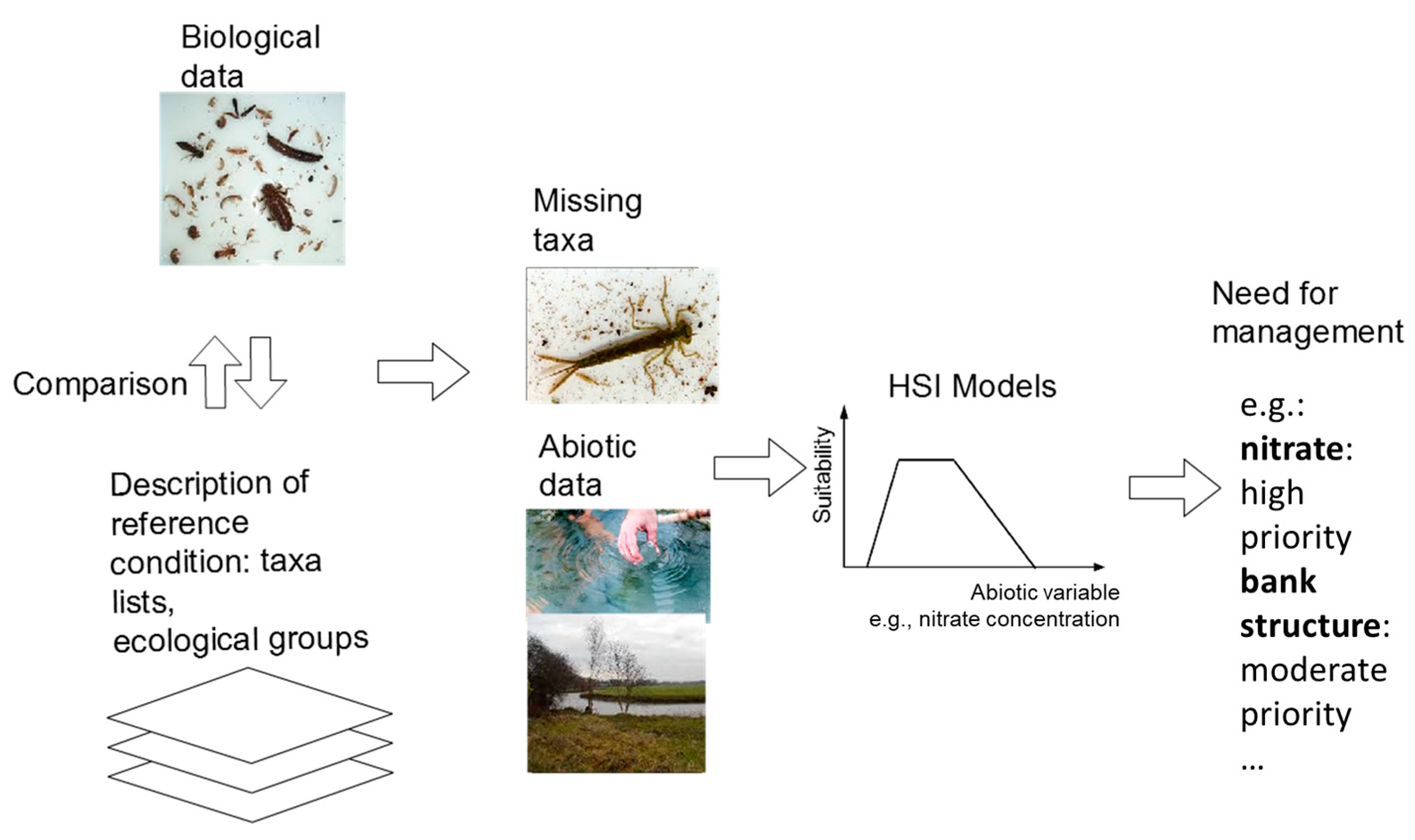
In our method, we use a set of suitability models for 92 macroinvertebrates as developed in Bennetsen et al. [22] in combination with biotic monitoring data, to classify aspects of river system according to their priority for management to restore the ecological status (Figure 1).
In a first step, we compared the biological community observed in a river to a list of taxa describing the operational Leitbild [26] to identify missing taxa that represent the ecological gap. Secondly, for all taxa in the operational Leitbild that are not present in the community currently observed, we calculate the suitability of the current abiotic conditions with their respective habitat suitability models. Input data for these models are physical–chemical and hydromorphological variables (Table SA3). All variables describe different aspects of a river system of which alterations of the natural condition could potentially pose a negative impact on the state of the water body. We then classify the resulting habitat suitabilities of each abiotic variables into different priority classes according to their need for management actions and to what degree they can be considered stressors.
In what follows, we first describe the construction of the operational Leitbild (Section 2.2) that the method uses to select the habitat suitability models to perform the analysis. This Leitbild represents a description of the desired situation per water body type, being the good ecological status. It consists of two elements: a description of the expected community in terms of ecological groups (Section 2.2.1), and a taxa list containing taxa that are members of these ecological groups (Section 2.2.2). We describe this operational Leitbild in terms of ecological groups because it allows one to reduce the number of Type I errors, where a taxon is classified as missing, even though another taxon sharing a similar ecological niche is present (thus indicating that the habitat is suitable for the taxon considered). For example, if a taxon A on the reference list is missing from the community observed and no other taxon from its ecological group is found in a sample, this taxon A is considered missing.
Next, we present the algorithm to apply the method (Section 2.3) and its evaluation (Section 2.4). We then describe the example application for the region of Flanders, Belgium (Section 2.5).
2.2. Defining an Operational Leitbild
2.2.1. Defining Ecological Groups
As the goal of our method is to provide information on the need for action to reach a good ecological status, it is not necessary that a current community exactly matches the ecological assemblage on our taxa lists. We consider these lists to be descriptions of an assemblage of species archetypes, in which each taxon on the list represents a specific ecological niche. Our goal was to reduce the number of Type I errors, where a taxon would be classified as missing, even though another taxon sharing a similar ecological niche was present. This could, for example, be the case as a different taxon sharing a similar niche would have a larger presence in the stream basin of the water body, than the taxon on our taxa list. Functionally, they would represent the same group of taxa, but taxonomically they differ. Using this method, we also avoided focusing on taxonomical composition alone. It can be seen as an approximation of functional diversity [28,29]. For this purpose, we defined a set of ecological groups, using data on ecological preferences from Verberk and Nijboer [30]. We therefore conducted a data-driven cluster analysis to identify clusters of taxa, similar to the analysis presented in Usseglio-Polatera et al. [31]. The aim of these clusters was to define ecological groups of taxa that have similar ecological preferences. The dataset contained autecological information for 2325 species for the following variables: trophic state, saprobic state, depth, velocity, substrate, salinity, water surface area, intermittent flow and acidity. This selection of ecological traits also align with the suggested categories presented by Mueller et al. [28]. Only taxa that are part of the taxa list considered in the MMIF calculation [27] were taken into consideration. We used divisive analysis clustering with a Gower coefficient as the dissimilarity index to construct a hierarchical clustering tree of species [32]. We specifically selected the Gower coefficient, as it can handle mixed data. The data on ecological traits are ordinal (fuzzy-coded). We set the maximum number of clusters to 20.
As the data in Verberk and Nijboer [30] were defined on the species level, and our data were defined on the genus or the family level, we had to aggregate the results to a higher taxonomic level. For each genus or family on our list of taxa, we determined the relative proportion of species in this taxon that was part of each group. We then assigned each taxon to the group with the highest proportion. To account for a loss of information in transforming these groups from a species level to a higher taxonomic level, we consulted three macroinvertebrate experts for Flanders. They were asked to check the proposed groups against the first criterion: similar ecological needs, but no assumed co-occurrence. The Flemish experts could also propose corrections to the original group compositions. We checked their propositions against the evidence that was provided by the cluster analysis (cfr. above). During the discussion, taxa were assigned to different groups by consensus.
2.2.2. Constructing the Taxa Lists Describing the Operational Leitbild
The reference condition for macroinvertebrates in Flanders has been defined based on expert judgment on the expected values of each metric in the MMIF by Gabriëls et al. [27]. Due to this, there are no taxa lists describing the expected community composition in each river type under reference conditions. Therefore, there are also no taxa lists describing the expected community at a good ecological status of each water body type. To overcome this, we developed lists of taxa for seven river types in Flanders, which describe the expected community composition under a good ecological status as defined by the MMIF. As the WFD requires member states the good ecological status the statutory requirement for water bodies, this is the desired situation and management endpoint for practitioners. Our taxa reference lists make a distinction between “base taxa”—generalist taxa that are generally present in this water body even at a lower than good ecological status—and “critical taxa”—sensitive taxa that only occur when a good ecological status is reached. The idea is that a good ecological status can only be reached with specific management that will lead to the (re)introduction of certain critical taxa in addition to these base taxa. These critical taxa are assumed to mainly occur in the good and high ecological status water bodies. This means that our benchmark describes a “least disturbed” or “best attainable condition” [33] rather than a “natural” or “historical” condition.
We developed the taxa lists using a dataset from the biological monitoring network of the Flanders Environment Agency. It contains 2910 samples between 2003 and 2012 describing the community composition observed at 714 sites in seven river types in Flanders. It also contains a classification of each sample according to the MMIF. Macroinvertebrate monitoring data were collected by kick sampling following De Pauw and Vanhooren [34]. The identification of the macroinvertebrates was carried out according to the taxonomic levels defined by Gabriels et al. [27], i.e., according to family, genus or another intermediate taxonomic level. A standardized list of taxa is provided in Gabriels et al. [27]. A full description of the datasets and the water quality status in the study area can be found in Tables SA1 and SA2.
We developed the taxa lists in two steps (Algorithm 1) to overcome the bias towards bad and poor ecological status in the dataset (Table SA1) and to avoid classifying sites focused on taxonomical composition alone. In the first step, we described the operational Leitbild by the species groups as were defined in Section 2.2.1. For this, we calculated the median and the mode of the number of individual taxa that were present per group at each sample with good or high ecological status. The median represents the typical number of taxa within each group that would be present at good ecological status. We then developed a list of candidate taxa with a data-driven analysis. To develop the initial list of candidate taxa, we calculated the fidelity score of each taxon to sites of a river type with a good or high ecological status. Fidelity is the degree to which a taxon prefers a water body type with a good or high ecological status, defined as the ratio of the relative frequency of a taxon in the subset of samples of sites in a river type with a good or high ecological status and their overall relative frequency [35]. We ranked the taxa according to their fidelity score, and for each river type we added the number of taxa per group as was calculated in the first step, starting with the taxon with the highest fidelity. This resulted in a first draft of the taxa list.
| Algorithm 1 Defining an operational Leitbild |
| Data: dataset with macroinvertebrate samples and their respective MMIF score from 2003 to 2012 |
| Result: taxa list describing the good ecological status per water body type |
| initialization; |
| FOREACH water body type W |
| FOREACH taxon t |
| Calculate number of occurrences O |
| IF O > 40 |
| Calculate Fidelity F for taxon t in all samples with MMIF ≥ 0.7 |
| END |
| END |
| FOREACH species group G |
| Calculate median M and mode Mo of the number of representatives of group G in all samples with MMIF ≥0.7 Select M taxa with the highest F from G and add to taxa list |
| END |
| Calculate MMIF mmifcal with taxa list using RA |
| WHILE mmifcal <0.7 |
| FOREACH metric that is too low for a good status |
| Select species group Gm that contributes to metric with the highest Mo and of which the number of taxa on the existing list is lower than its respective Mo |
| Select taxon t with the next highest F from Gm and add to taxa list |
| END |
| Calculate MMIF mmifcal with taxa list using RA |
| END |
| END |
In a second step, we made sure that the taxa lists actually described a good ecological status, by calculating the expected MMIF with these taxa present (Section SB1). The MMIF is calculated using 5 submetrics: the number of taxa, the number of sensitive taxa, the mean tolerance score, the Shannon–Wiener index and the number of taxa from the group of Ephemeroptera, Plecoptera or Trichoptera [27]. If the MMIF for the proposed list of taxa did not reach 0.7 (the cutoff for a good ecological status) for a water body type, we reviewed the submetric values to assess which metric caused the lower MMIF value. If necessary we added one extra taxon from an ecological group to the list for that water body type, which would correct this submetric. When multiple groups were possible, we chose the group for which the mode of this group in this water body type was higher than the median as calculated above. We then iteratively went through this procedure until the MMIF associated with the taxa list for each water body type reached minimally 0.7. Furthermore, only taxa that had more than 40 occurrences in the dataset were considered, as there were no models for taxa with lower occurrences [22].
Taxa with a tolerance score lower than 6 (not very sensitive to pollution) were considered base taxa. Taxa with a tolerance score of 6 or higher were considered critical taxa. This threshold coincides with the threshold related to the submetric number of sensitive taxa in the MMIF calculation [27].
2.3. Classifying Aspects of a River System into Priority Classes
Our method uses a set of suitability models as presented in Bennetsen et al. [22]. We based the model development on ecological theory and calibrated the models using Flemish monitoring data and databases with ecological knowledge. We quantified the added value of incorporating ecological theory and knowledge on ecological preferences. One model for one taxon consists of different non-symmetric unimodal trapezoid functions describing the univariate suitability per abiotic variable. This simplification of the typical bell-shaped curve makes it possible to describe various types of distributions with different degrees of skewness and kurtosis [36]. For a detailed description of the model development, we refer to Bennetsen et al. [22]. A list of all input variables can be found in Table SA3. All input variables are variables describing the state of a water body. All variables included in the models have legal targets defined. When they deviate from the legal target and can be related to pressures in the water body system, they can potentially be considered a stressor. All hydromorphological variables included are defined as ordinal variables describing the degree of alteration of its state from the expected natural condition [22].
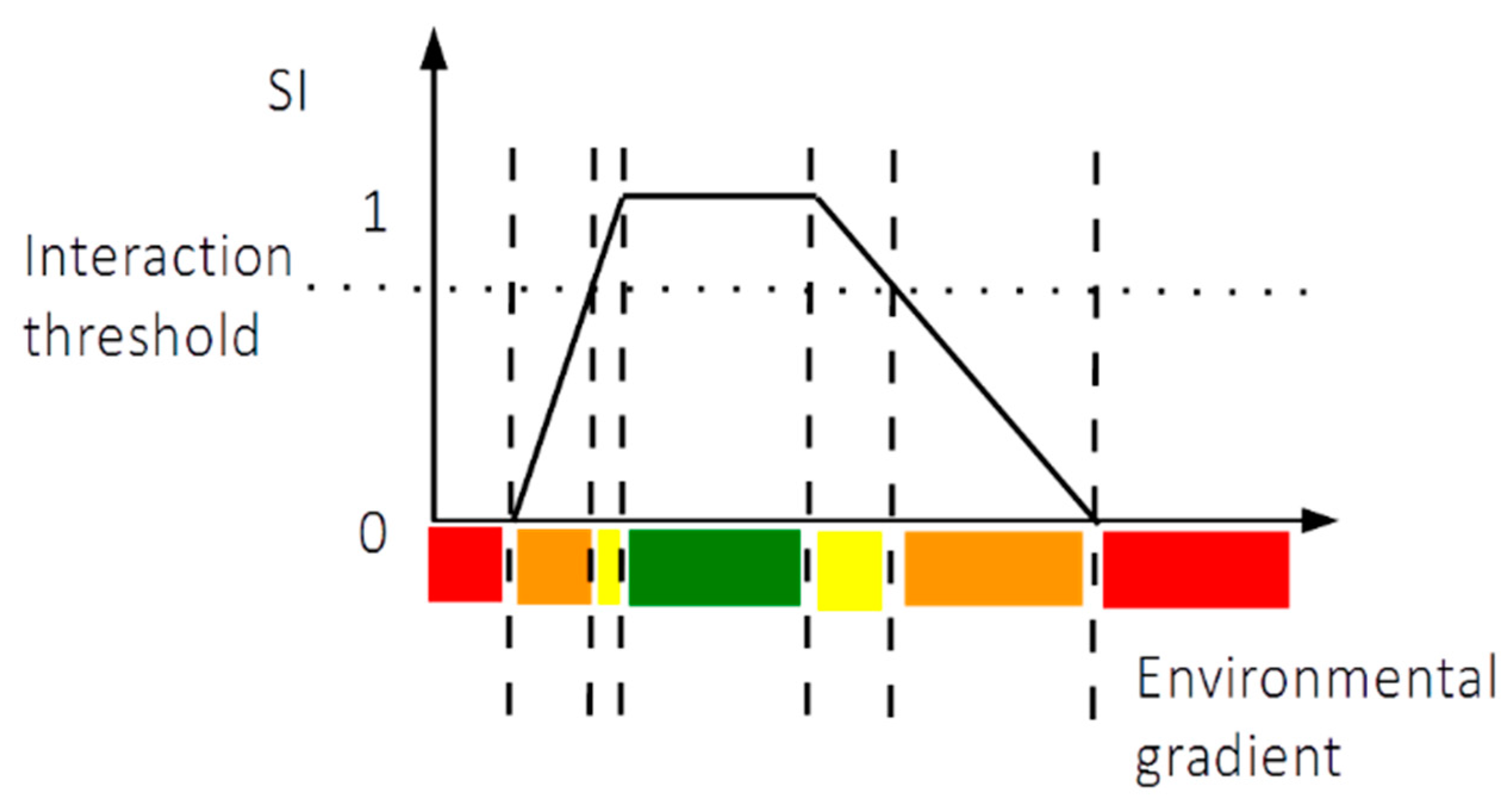
To define the priority class for each stressor (Algorithm 2), the current community is first compared to the taxa lists defined in Section 2.2. To identify a taxon as missing, we first compare the community observed in terms of ecological groups. If in the community observed the number of taxa in an ecological group is lower than the number of taxa in this ecological group on the reference list, this amount of taxa is considered missing. This number represents the ecological gap. In a second step, we selected from the taxa list this number of taxa per ecological group. These are referred to as the missing taxa. These will be the taxa for which we used the suitability models in the priority classification. These selected taxa cannot be present in the community observed. For each missing taxon, we then calculated the suitability index SI for each abiotic variable. This SI was quantified as a score between 0 and 1, which we divided into four priority classes. Each of these classes represents the need for management for each abiotic variable (Figure 2). In the first class (SI = 0, “Out of range, needs action”), a variable is out of range of suitability for a taxon, meaning that it poses an important pressure on the biological status and can be considered a stressor. The good ecological status cannot be reached unless this stressor is addressed. In the second class (0 < SI ≤ cutoff value, “Consider action”), the site has low habitat suitability for this abiotic variable. In this range, the degree to which this aspect of a river system can be considered a stressor depends on the interaction between different variables of lower suitability for this taxon. The cutoff for this suitability value is derived from the so-called interaction threshold as calibrated in Bennetsen et al. [22]. This interaction threshold represents the idea that if the suitability is low according to many variables, the likelihood that a taxon can be present decreases. In the third class (cutoff value < SI < 1, “Flagged”), a variable is suboptimal, which indicates that this variable probably does not pose an important stressor and should not be addressed with a high priority even if it deviates from its legal target. Still, there may be a risk for rapid deterioration when its value changes due to an incident or unexpected effected of management interventions. In the fourth case (SI = 1, “No action needed”), the habitat, according to this variable, is considered as suitable, which means that it is not a stressor and that it should not be taken into account when planning management actions in this river for macroinvertebrates.
| Algorithm 2 Defining priority classes for individual abiotic variables |
| Data: dataset with macroinvertebrate samples, their respective abiotic conditions and their respective MMIF score from 2010–2012 D; taxa list describing a reference condition per water body type TL; a set of habitat suitability models HSM |
| Result: description of missing taxa; classification of priorities |
| initialization; |
| FOREACH sample S in D |
| IF MMIF ≥ 0.7 |
| Set number of missing taxa to 0 NMT Set priority P for all abiotic variables to 0 |
| ELSE |
| Identify missing taxa TM Count number of missing taxa NMT |
| FOREACH TM and abiotic variable AV |
| Calculate suitability index SI |
| IF SI = 0 |
| Set priority P to 0 |
| ELSE IF SI < cutoff value CV & CV! = 1 |
| Set priority P to 1 |
| ELSE IF SI < 1 |
| Set priority P to 2 |
| ELSE IF SI = 1 |
| Set priority P to 3 |
| END |
| END |
| FOREACH abiotic variable AV |
| Priority Class PC = floor(weighted harmonic mean (P)) with weight = 1|2 for respectively base and critical taxa |
| END |
| END |
| END |
To obtain a priority class for each variable per water body, we aggregated the priority classes per variable and per missing taxon using a weighted harmonic mean. Critical taxa receive double the weight of base taxa. As we used the harmonic mean, taxa for which the variable has a lower suitability would have more impact on the final value for classification [37]. The aggregated priority scores were rounded to their lowest integer value and were coded into the same four classes as the individual classes. This results in a classification of each aspect of the river system of each water body in the dataset.
2.4. Evaluation of Our Method
Each individual suitability model was validated and tested as described in Bennetsen et al. [22]. We further tested our method, by calculating the expected MMIF by executing a simulation of the models developed in Bennetsen et al. [22] for the taxa that were included in the reference list, using a test dataset that was not used in model development, with data gathered from 2003 to 2012. For this we used the method described in Section B1 in supportive information. We compared this simulated MMIF value with the true MMIF, by constructing the confusion matrix on the classified MMIF and calculating Cohen’s Kappa and the accuracy. We also compared the accuracy to the no information rate (NIR), which is the proportion of the most prevalent class in the test dataset. The accuracy should be higher than this NIR to be acceptable [38]. For the MMIF value, we also calculated the RMSE.
We also calculated the Pearson correlation of the number of missing taxa and the number variables with a priority class of 0 or 1 to the MMIF score.
2.5. Example Application: The Case of Flanders
We illustrate our method by applying it to a dataset of sampling data from 381 monitoring points collected between 2010 and 2012 in Flemish water bodies and local water bodies of the 1st order. To compile the abiotic input dataset, we coupled the biotic monitoring data to the statistical derivative of the physical–chemical abiotic data, as used for assessing water quality against the water quality norms in Flanders (Table SA2) and the hydromorphological observations reported for each water body. The statistical derivatives represent an overall view of the water quality per water body for the full year. All data were obtained from the WFD monitoring network run by the Flanders Environment Agency [39]. A full description of the dataset and the water quality status in the study areas can be found in Table SA2.
3. Results
3.1. Defining the Operational Leitbild
3.1.1. Ecological Groups
The ecological groups represents groups of taxa that have similar habitat needs, but do not necessarily co-occur. Based on the hierarchical cluster analysis and the expert consultation, we identified 16 ecological groups (Table SC1). Table 1 gives an overview of the final taxonomic composition of each group, and how many taxa were assigned to each group. The groups are mainly clustered on the ecological preferences, and the tolerance scores as defined in Gabriëls et al. [27]. However, some taxonomical clustering is also observed.
3.1.2. Taxa Lists
The final taxa lists (Table SC2) describe community assemblages with 25–30 taxa. Of these taxa, between 35% and 45% of taxa were identified as critical taxa, with a high fidelity score to the good water quality class. The distinction between critical taxa and base taxa is reflected in the tolerance scores as defined by Gabriëls et al. [27]. Critical taxa have a tolerance score of 6 and above, indicating high sensitivity to pollution.
3.2. Evaluation of the Method
Using the suitability models defined in Bennetsen et al. [22] for the taxa on the lists describing the operational Leitbild, we validated the predictive power of the models for the MMIF classification and score on a dataset independent from the dataset used in model development. Of all samples 47.7% were correctly classified, Cohen’s Kappa was 0.26 (p = 0.05) and the RMSE value on the MMIF score was 0.18. This accuracy was higher than the no information rate 32.96% (p = 0.008).
There is a monotonic decreasing relationship between the results of the priority classification and the ecological status expressed as the MMIF. The number of variables that have a low to high priority was negatively correlated with the MMIF score of the water body (r = −0.72, p < 0.001). The number of missing taxa (median count 14) was negatively correlated (r = −0.92, p < 0.001) with the MMIF value of the water body. If no ecological groups were considered, more missing taxa (median count 18) were identified. In this case the correlation of the number of missing taxa to the MMIF score would drop to −0.86 (Pearson correlation coefficient, p < 0.001).
3.3. Example Application: The Case of Flanders
The application of our method on the regional level of Flanders illustrates how the ecological status can serve as a classifier to determine the priority of management of different aspects of a river system (Table 2). Overall, hydromorphological variables were almost never classified as being out of range, except variables related to the profile (width and depth) and the presence of sediment banks. Physical–chemical variables were classified in on average 15% of cases as being out of range. The variables with the highest priority in Flanders are electrical conductivity (28%), Kjeldahl nitrogen concentration (25%) and nitrate concentration (19%). Some variables are mostly classified as “consider action”, because of lower suitability, such as the presence of plants (46%) and width variation (50%). The variables that are most often classified as suboptimal are: presence of dead wood (84%), variables related to stream patterns (pool-riffle pattern (69%) and stream variation (64%)). Only depth is to a high degree classified as having no need for action (60%).
The legal targets set for physical–chemical and hydromorphological variables can differ from the results of the priority classification (Table 2). For example, in 25% of samples the biological oxygen demand complies with its legal target, but according to our model results, there is still a need for action. On the other hand, there are water bodies whose profile has been modified, resulting in a non-compliance for the width-to-depth ratio with the legal target, yet the width and depth of these water bodies do not require action in respectively 19% and 29% of those samples for macroinvertebrates.
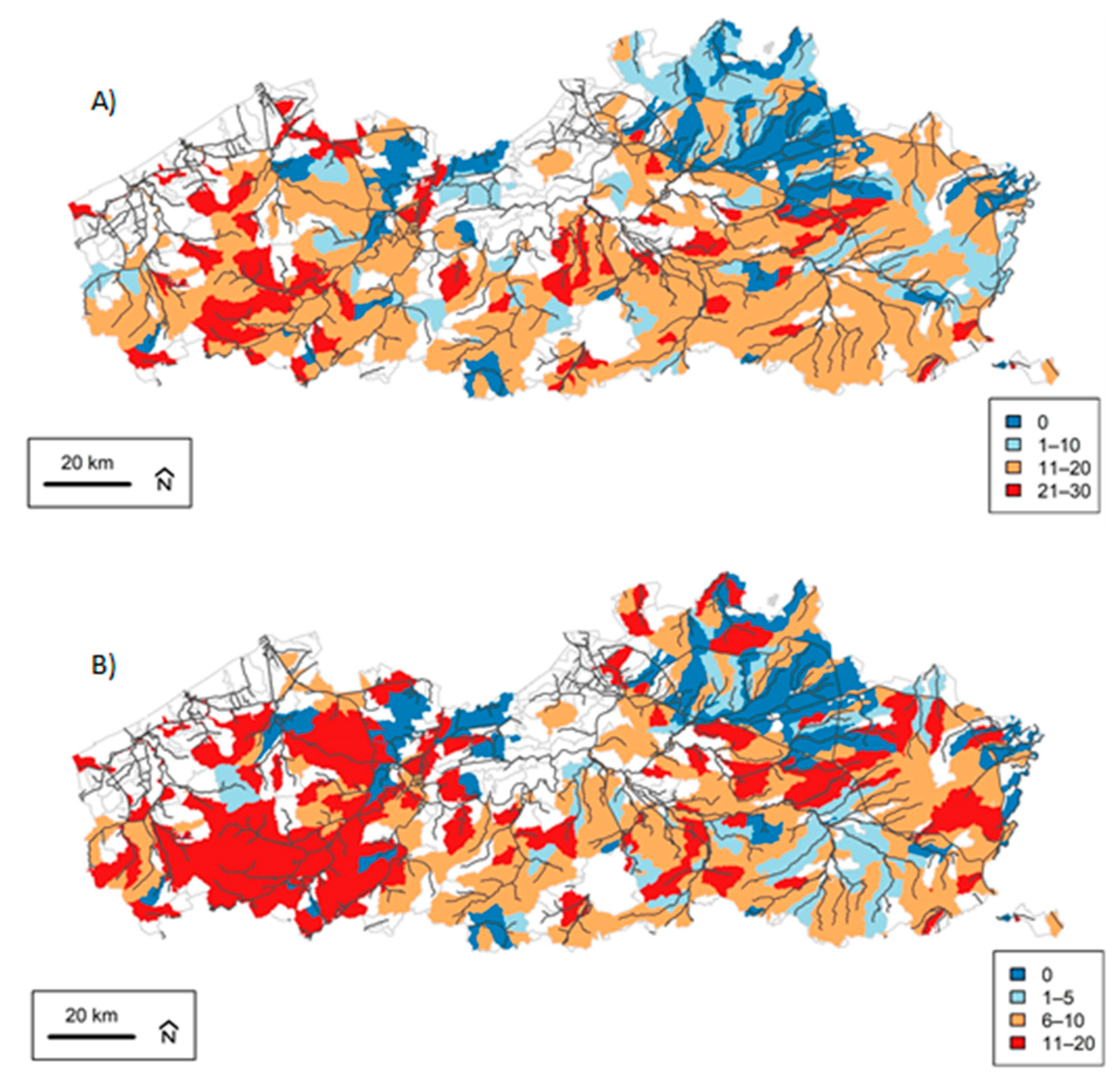
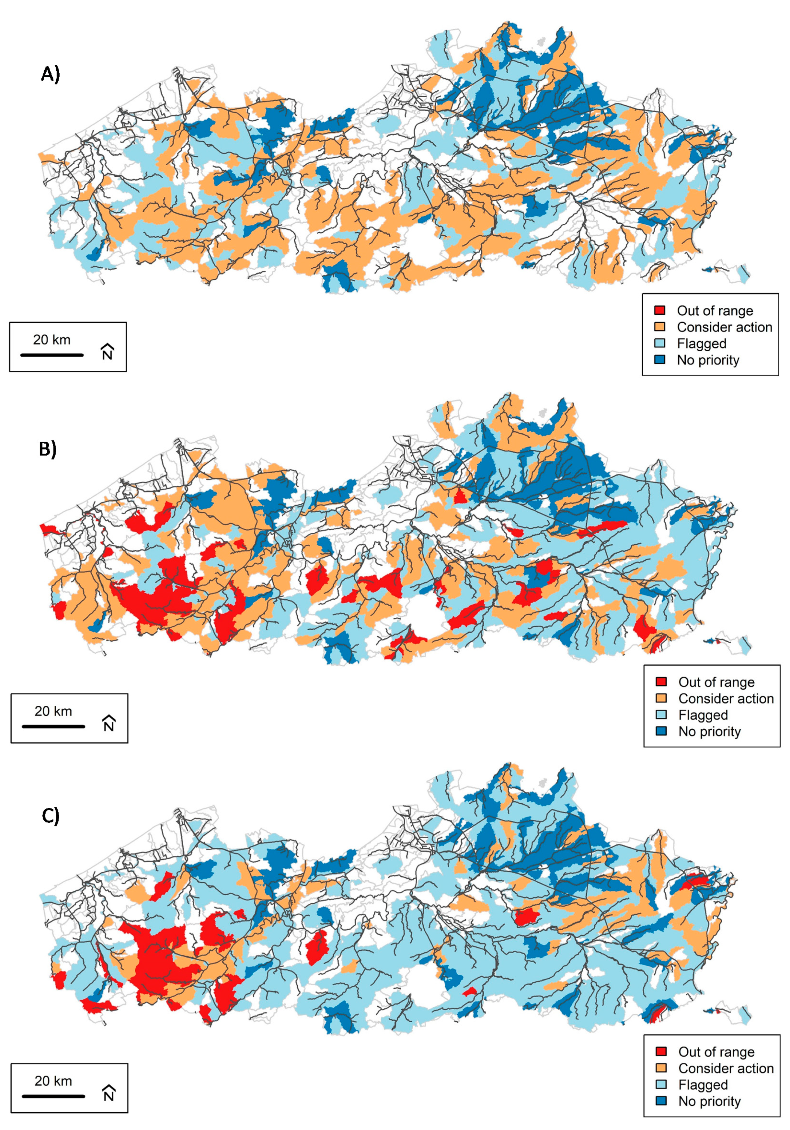
On average, 13 missing taxa were identified, and 9 variables were classified as in need of action (Figure 3A,B). There is a gradient in the number of missing taxa and in the number of limiting variables from west to east, which coincides with the gradient of the MMIF from west to east (Figure SD1). There are regional differences between the ways in which each stressor is classified according to their need for management (Figure 4A–C). Width variation is classified as “consider action” in smaller subsidiaries of larger water bodies. Biological oxygen demand can be of high priority all throughout Flanders, while orthophosphate phosphorus concentration specifically needs to be addressed in the westside of the region.
4. Discussion
4.1. Method Development
In this paper, we presented a method for classifying individual aspects of a river system according to their need for management, combining insights from biological monitoring and ecological modeling. The goal was to increase the value of individual biological measurements as explanatory tools, when planning for management actions in river restoration. To this end, we disassembled the biotic index for macroinvertebrates, the MMIF, into its individual building blocks.
The results of our method had a good correlation with MMIF values. Both the number of missing taxa identified from the reference lists, and the number of stressors identified have a good correlation with the MMIF. The monotonic negative correlation of the MMIF with the number of missing taxa identified strengthens from −0.86 to −0.92 when ecological groups are included in this step. Hence, the inclusion of ecological groups reduces the number of type I errors in our classification exercise. This reduces the risk of considering an aspect of a river system as a stressor, when no management action is needed, a reduction that can result in more cost-effective management [40]. Furthermore, the composition of the ecological groups is consistent with ecological preferences and to a lesser extent with taxonomical composition, but the latter is not a prerequisite for the purpose of this tool [41]. The combination of the taxa reference lists with the ecological groups can be linked to the idea of species surrogates for a good ecological status [42]. For inclusion of candidate taxa on the taxa lists describing the operational Leitbild, we considered both samples with a good and high ecological status in the dataset. This increased the applicability of the integrated model, as, in practice, a good ecological status will be considered the first management endpoint for seeking compliance with the WFD [6].
Bennetsen et al. [22] indicate that there is a good relationship between the performance of the suitability models used and the inclusion of ecological knowledge in the construction of the models. For example, compared to the use of threshold indicator taxa analysis (TITAN) to detect change points [43], both the average sensitivity (0.57 vs. 0.48) and specificity (0.87 vs. 0.67) for the prediction of species occurrence are higher. Furthermore, using the habitat suitability models from Bennetsen et al. [22], we assessed the predictive power for the MMIF of the models used. The accuracy of our models (47.7%) is within of the interval of accuracy (45–57%) presented when classifying the MMIF score directly with classification trees [44]. Major advantages of the presented method are the insights that are gained in the shifts in community aspects (diversity, tolerance and specific groups), which types of invertebrates are likely to occur or disappear as a consequence of changes in abiotic conditions and moreover an improved insight related to the uncertainty in the models and their predictions.
4.2. Example Application: The Case of Flanders
Our method is successful in identifying the most important stressors in water bodies. It also allows the detection of regional differences. For example, the importance of orthophosphate concentration decreases when going from west to east in Flanders. This could be explained by a decreasing proportion of agricultural and urban land use from the west to the east (Section SA). Furthermore, the results also show a distinction between small and large water bodies in terms of priorities. In smaller water bodies, hydromorphological variables such as the presence of width variation have a higher importance than in larger water bodies. The presence of width variation can be considered an indicator of the presence of diversity in microhabitats, like in, for example, a sequence of slow and fast flowing segments, and is expected to be higher in smaller water bodies, than in larger ones [45]. The diversity in microhabitats has been shown to be important for macroinvertebrates in streams [46]. Overall, physical–chemical variables seem to require a higher priority than hydromorphological variables, which coincides with insights in the literature [9,47,48]. Yet, many hydromorphological variables, such as the presence of water-related elements, the presence of macrophytes, the presence of natural erosion processes and the profile of a stream (width-to-depth ratio and width variation) are classified as “consider action” in between 30 and 50% of all water bodies. Many water bodies in Flanders are artificial or have been heavily modified, which is reflected in the moderate priority of channel processes that reflect habitat diversity in a watercourse, such as erosion processes and bedding vegetation.
4.3. Relationship of Our Method to Legal Targets
The results of our integrated model indicate that taxon specific responses have a different sensitivity to identify stressors than indicated by the legal targets set for physical–chemical and hydromorphological variables. The norms for these quality elements are based on supporting the ecological status [6], but the number of sites that are selected as being priority sites for management differ from the number of sites that do not comply with the norms in the WFD [39]. Hence, for reaching a good ecological status, river managers should not only focus on the compliance of individual elements, but rather consider a systems approach to the catchment [6]. This is possible as there are 48 sites that have a “good” MMIF status, whose physical–chemical status is poor to moderate, and there are 10 sites whose physical–chemical status is “good” and MMIF is only moderate. This is corroborated by studies such as Sundermann et al. [7], who argue that these norms should be considered ecological background values, not change point values for biological groups. This does not mean that these legal targets have no basis, as they are supportive of more biological groups than macroinvertebrates alone.
Our method is not the only method with which taxon-specific tipping points could be defined, there are examples with taxon-specific analyses using the TITAN algorithm [7]. Even the breakpoints in the classification trees relating directly to the MMIF [44,49] could inform on change points specific to macroinvertebrates. Our method differs from these other change point detecting method by assigning a fuzzy classification to these change points. When a suitability index is either 0 or 1, the classification for the need of management is clear-cut, but when habitat suitability is between 0 and 1, this makes for a grayer zone. There might or might not be a need for management. We introduce a more risk-based approach in which aspects of a river system that are altered to a degree that they result in a lower habitat suitability, are designated as “consider action”, and variables with a higher suitability are “flagged”. This informs river managers on uncertainty and allows for expert judgment on these aspects in local cases, using knowledge of stakeholders and river managers that cannot easily be captured in desktop analyses. This could increase the acceptance of our method by stakeholders and river managers [50]. Yet it still makes it possible to screen different aspects of river systems on regional differences in terms of their negative impact on the biological status, without further expert judgment.
4.4. Possible Applications of the Method
The most important application of our method is that of turning a bulk of measurement data into structured information for river managers. This allows for setting regional priorities and local priorities: which areas should we address first, and what aspects? Our method has similarities to that proposed by De Zwart et al. [51]. A more typical use of the habitat suitability models as presented in Bennetsen et al. [22] would be to assess the effect of different water quality management scenarios, by integrating them as the last set of models in an integrated modeling chain with other water quality models. However, we think that such an integrated modeling framework overlooks a crucial step in planning and decision support: how can we design management scenarios? To test a great number of different scenarios with water quality models can be very time-consuming, either owing to computational time and requirements, or to the sheer complexity of preparing the various input data. To reduce the number of scenarios that should be tested with water quality models, a crucial first step is something that can be referred to as solution scanning [52]. By first analyzing the system and making a diagnosis [5] of the impairment at hand, river managers can specify a limited set of management options [53] that could be tested in scenario calculations with perhaps more complex water quality models. Due to this, we argue to not only put the ecological models as the last model in an integrated modeling framework, but to use them also as a first step in these frameworks. There is of course logic to putting these models last, as they typically represent the management endpoint within integrated water management. However, as other authors and we [7] have illustrated, ecological responses do not always align with information derived from legal targets. Performing an ecological data analysis first makes it possible to perform a gap analysis sensitive to ecological responses. Thus, by putting the ecological models first, our method aligns with the argument for a true systems approach in integrated water management [6].
4.5. Outlook and Future Development
Our method is able to identify different types of stressors, has a good relationship with the ecological status and is flexible in terms of target setting for river restoration. As each individual aspect of a river system is classified individually, it would for example also be possible to run these models on incomplete data, with the indication that on these aspects no information is available.
Yet its univariate character is a potential disadvantage of our method, as no interaction between stressors is identified in our calculations. However, as the interaction value, used to designate variables either as “consider action” or “flagged”, is based on the multivariate interaction between different stressors [22], interactions are nevertheless considered, albeit indirectly. Yet a possible improvement to the method would be an input variable selection, for example using genetic algorithms [36], to reduce the number of input variables, which would make the consideration of interactions between stressors a less complex problem.
The method presented in this paper used an operational Leitbild developed using data from 2003 to 2012 for an application on a dataset from 2010 to 2012. To apply the method in the future on more recent data, or in different regions, it is advised to update this Leitbild with more recent biological data or data from that specific region to ensure that it describes the expected community under a good ecological status in terms of taxa that have a strong presence in the region and period considered. This will ensure that the results of the classification are the most relevant to the most important taxa in the area at that time.
Furthermore, dispersal or the recolonization potential is not considered in the method presented in this paper. Yet model performance improved significantly when a simple dispersal metric was included in the initial model development [22]. Recently, several authors have indicated the importance of recolonization potential in planning ecological river restoration [54,55]. There are also water bodies in our example application with large ecological gaps, indicating many missing taxa for a good water ecological status, but where water quality is nevertheless good. Perhaps a better explanation than individual stressors would be the absence of source populations for these water bodies [55]. Furthermore, by combining our method with that proposed in Dahm et al. [56], water bodies that have a high potential of reaching good water quality status immediately after river restoration could be identified, and thus prioritized spatially.
5. Conclusions
In this study, we aimed to combine suitability models with information on the ecological status to classify aspects of a river system as potential stressors according to their need for management. We showed that disassembling the ecological status into its individual building blocks has great potential to integrate the ecological status from a systems perspective into models supporting the WFD implementation and integrated water management in general. Specifically, our method considers the ecological status not only as an endpoint in decision support modeling to evaluate scenarios, but also considers it the starting point for a diagnostic analysis related to the pressure and impact analysis. More in particular, we found that the results of our method correlate well with other biotic index studies, and that our method adds new knowledge on the following points: (1) our explicit inclusion of ecological theory and knowledge makes it possible to disassemble biotic indices into their individual building blocks and (2) this approach allows a fuzzy classification of aspects of a river system as potential stressors and their priority for management, which allows expert judgment in local cases. Thus, our method is beneficial to currently used methods directly relating information to the biotic index.
The method presented results in a solid classification of individual aspects of a river system according to their priority for management. It can be supporting of the pressure-impact analyses of water bodies and in the design of a river restoration plan. The inclusion of ecological knowledge and expert insight improves the ecological soundness of the individual elements and the reliability of the method. It also results in good confidence in the prioritization of stressors, despite a moderate predictive performance of the underlying models. We presented the application of our model for Flanders and only for macroinvertebrates, but the principles of the method can be implemented in any region and with other underlying models.
Supplementary Materials
The following are available online at https://www.mdpi.com/article/10.3390/w13070886/s1. Table SA1: Number of samples per river type and per ecological quality class, Table SA2: Percentage of samples per quality class for the ecological status based on macroinvertebrates, the physical-chemical status and the hydromorphological status, Table SA3: Overview of the input variables of the suitability models, Figure SB1: Macroinvertebrate taxa in Flanders ranked according to their 95th percentile abundance value in the monitoring data, Table SB1: Overview of the abundance classes, Table SC1: Composition of ecological groups, Table SC2: Taxa reference lists with base (B) and critical (C) taxa, Figure SD: Spatial visualization of all the priority classes of all variables considered in the case study of Flanders.
Author Contributions
Conceptualization, E.B., S.G., G.E. and P.G.; methodology, E.B., S.G., G.E. and P.G.; software, S.G. and E.B.; validation, E.B., S.G. and P.G.; formal analysis, E.B. and S.G.; writing—original draft preparation, E.B.; writing—review and editing, P.G., S.G., G.E. and E.B.; visualization, E.B. and S.G.; supervision, P.G.; project administration, P.G.; funding acquisition, P.G. All authors have read and agreed to the published version of the manuscript.
Funding
This research was funded by the Flanders Environment Agency, study, N° VMM/SGB/002/2012.
Institutional Review Board Statement
Not applicable.
Informed Consent Statement
Not applicable.
Data Availability Statement
Restrictions apply to the availability of these data. Data was obtained from the Flanders Environment Agency and are available at https://www.integraalwaterbeleid.be/nl/geoloket/geoloket-stroomgebiedbeheerplannen with the permission of the Flanders Environment Agency.
Acknowledgments
The authors would like to acknowledge Rob Laethem and Tom D’heygere for the fruitful discussions during the research project.
Conflicts of Interest
The authors declare no conflict of interest. The funders had no role in the design of the study; in the collection, analyses, or interpretation of data; in the writing of the manuscript, or in the decision to publish the results.
References
- Vorosmarty, C.J.; McIntyre, P.B.; Gessner, M.O.; Dudgeon, D.; Prusevich, A.; Green, P.; Glidden, S.; Bunn, S.E.; Sullivan, C.A.; Liermann, C.R.; et al. Global Threats to Human Water Security and River Biodiversity. Nature 2010, 467, 555–561. [Google Scholar] [CrossRef]
- Allan, J.D. Landscapes and Riverscapes: The Influence of Land Use on Stream Ecosystems. Annu. Rev. Ecol. Evol. Syst. 2004, 35, 257–284. [Google Scholar] [CrossRef]
- Jansson, R.; Nilsson, C.; Malmqvist, B. Restoring Freshwater Ecosystems in Riverine Landscapes: The Roles of Connectivity and Recovery Processes. Freshw. Biol. 2007, 52, 589–596. [Google Scholar] [CrossRef]
- Bernhardt, E.S.; Palmer, M.A. River Restoration: The Fuzzy Logic of Repairing Reaches to Reverse Catchment Scale Degradation. Ecol. Appl. 2011, 21, 1926–1931. [Google Scholar] [CrossRef]
- Elosegi, A.; Gessner, M.O.; Young, R.G. River Doctors: Learning from Medicine to Improve Ecosystem Management. Sci. Total Environ. 2017, 595, 294–302. [Google Scholar] [CrossRef] [PubMed]
- Voulvoulis, N.; Arpon, K.D.; Giakoumis, T. The EU Water Framework Directive: From Great Expectations to Problems with Implementation. Sci. Total Environ. 2017, 575, 358–366. [Google Scholar] [CrossRef]
- Sundermann, A.; Leps, M.; Leisner, S.; Haase, P. Taxon-Specific Physico-Chemical Change Points for Stream Benthic Invertebrates. Ecol. Indic. 2015, 57, 314–323. [Google Scholar] [CrossRef]
- Bouleau, G.; Pont, D. Did You Say Reference Conditions? Ecological and Socio-Economic Perspectives on the European Water Framework Directive. Environ. Sci. Policy 2015, 47, 32–41. [Google Scholar] [CrossRef]
- Dahm, V.; Hering, D.; Nemitz, D.; Graf, W.; Schmidt-Kloiber, A.; Leitner, P.; Melcher, A.; Feld, C.K. Effects of Physico-Chemistry, Land Use and Hydromorphology on Three Riverine Organism Groups: A Comparative Analysis with Monitoring Data from Germany and Austria. Hydrobiologia 2013, 704, 389–415. [Google Scholar] [CrossRef]
- Friberg, N.; Bonada, N.; Bradley, D.C.; Dunbar, M.J.; Edwards, F.K.; Grey, J.; Hayes, R.B.; Hildrew, A.G.; Lamouroux, N.; Trimmer, M.; et al. Biomonitoring of Human Impacts in Freshwater Ecosystems. In Advances in Ecological Research; Elsevier: Amsterdam, The Netherlands, 2011; Volume 44, pp. 1–68. ISBN 978-0-12-374794-5. [Google Scholar]
- Birk, S.; Bonne, W.; Borja, A.; Brucet, S.; Courrat, A.; Poikane, S.; Solimini, A.; van de Bund, W.; Zampoukas, N.; Hering, D. Three Hundred Ways to Assess Europe’s Surface Waters: An Almost Complete Overview of Biological Methods to Implement the Water Framework Directive. Ecol. Indic. 2012, 18, 31–41. [Google Scholar] [CrossRef]
- Brown, E.D.; Williams, B.K. Ecological Integrity Assessment as a Metric of Biodiversity: Are We Measuring What We Say We Are? Biodivers. Conserv. 2016, 25, 1011–1035. [Google Scholar] [CrossRef]
- Carré, C.; Meybeck, M.; Esculier, F. The Water Framework Directive’s “Percentage of Surface Water Bodies at Good Status”: Unveiling the Hidden Side of a “Hyperindicator”. Ecol. Indic. 2017, 78, 371–380. [Google Scholar] [CrossRef]
- Verberk, W.; van Noordwijk, C.; Hildrew, A. Delivering on a Promise: Integrating Species Traits to Transform Descriptive Community Ecology into a Predictive Science. Freshw. Sci. 2013, 32, 531–547. [Google Scholar] [CrossRef]
- Schuwirth, N.; Reichert, P. Bridging the Gap between Theoretical Ecology and Real Ecosystems: Modeling Invertebrate Community Composition in Streams. Ecology 2013, 94, 368–379. [Google Scholar] [CrossRef] [PubMed]
- Clews, E.; Ormerod, S.J. Improving Bio-Diagnostic Monitoring Using Simple Combinations of Standard Biotic Indices. River Res. Appl. 2009, 25, 348–361. [Google Scholar] [CrossRef]
- Holguin Gonzalez, J.E.; Everaert, G.; Benedetti, L.; Amerlinck, Y.; Goethals, P.L.M. Use of Habitat Suitability Modeling in the Integrated Urban Water System Modeling of the Drava River (Varazdin, Croatia). In Proceedings of the 9th International Symposium on Ecohydraulics (ISE 2012), Vienna, Austria, 17–21 September 2012. [Google Scholar]
- Klauer, B.; Rode, M.; Schiller, J.; Franko, U.; Mewes, M. Decision Support for the Selection of Measures According to the Requirements of the EU Water Framework Directive. Water Resour. Manag. 2012, 26, 775–798. [Google Scholar] [CrossRef]
- Villeneuve, B.; Souchon, Y.; Usseglio-Polatera, P.; Ferréol, M.; Valette, L. Can We Predict Biological Condition of Stream Ecosystems? A Multi-Stressors Approach Linking Three Biological Indices to Physico-Chemistry, Hydromorphology and Land Use. Ecol. Indic. 2015, 48, 88–98. [Google Scholar] [CrossRef]
- Bizzi, S.; Surridge, B.W.J.; Lerner, D.N. Structural equation modelling: A novel statistical framework for exploring the spatial distribution of benthic macroinvertebrates in riverine ecosystems: Benthic macroinvertebrate distributions through SEM. River Res. Appl. 2013, 29, 743–759. [Google Scholar] [CrossRef]
- Kuemmerlen, M.; Stoll, S.; Sundermann, A.; Haase, P. Long-Term Monitoring Data Meet Freshwater Species Distribution Models: Lessons from an LTER-Site. Ecol. Indic. 2016, 65, 122–132. [Google Scholar] [CrossRef]
- Bennetsen, E.; Gobeyn, S.; Goethals, P.L.M. Species Distribution Models Grounded in Ecological Theory for Decision Support in River Management. Ecol. Model. 2016, 325, 1–12. [Google Scholar] [CrossRef]
- Jähnig, S.C.; Kuemmerlen, M.; Kiesel, J.; Domisch, S.; Cai, Q.; Schmalz, B.; Fohrer, N. Modelling of Riverine Ecosystems by Integrating Models: Conceptual Approach, a Case Study and Research Agenda. J. Biogeogr. 2012, 39, 2253–2263. [Google Scholar] [CrossRef]
- D’Amen, M.; Mateo, R.G.; Pottier, J.; Thuiller, W.; Maiorano, L.; Pellissier, L.; Ndiribe, C.; Salamin, N.; Guisan, A. Improving Spatial Predictions of Taxonomic, Functional and Phylogenetic Diversity. J. Ecol. 2018, 106, 76–86. [Google Scholar] [CrossRef]
- Guisan, A.; Tingley, R.; Baumgartner, J.B.; Naujokaitis-Lewis, I.; Sutcliffe, P.R.; Tulloch, A.I.T.; Regan, T.J.; Brotons, L.; McDonald-Madden, E.; Mantyka-Pringle, C.; et al. Predicting Species Distributions for Conservation Decisions. Ecol. Lett. 2013, 16, 1424–1435. [Google Scholar] [CrossRef] [PubMed]
- Jungwirth, M.; Muhar, S.; Schmutz, S. Re-Establishing and Assessing Ecological Integrity in Riverine Landscapes. Freshw. Biol. 2002, 47, 867–887. [Google Scholar] [CrossRef]
- Gabriels, W.; Lock, K.; De Pauw, N.; Goethals, P.L.M. Multimetric Macroinvertebrate Index Flanders (MMIF) for Biological Assessment of Rivers and Lakes in Flanders (Belgium). Limnol. Ecol. Manag. Inland Waters 2010, 40, 199–207. [Google Scholar] [CrossRef]
- Mueller, M.; Pander, J.; Geist, J. Taxonomic Sufficiency in Freshwater Ecosystems: Effects of Taxonomic Resolution, Functional Traits, and Data Transformation. Freshw. Sci. 2013, 32, 762–778. [Google Scholar] [CrossRef]
- Péru, N.; Dolédec, S. From Compositional to Functional Biodiversity Metrics in Bioassessment: A Case Study Using Stream Macroinvertebrate Communities. Ecol. Indic. 2010, 10, 1025–1036. [Google Scholar] [CrossRef]
- Verberk, W.C.; Nijboer, R.C. Milieu-En Habitatpreferenties van Nederlandse Zoetwatermacrofauna; STOWA: Engelsbrand, Germany, 2012. [Google Scholar]
- Usseglio-Polatera, P.; Bournaud, M.; Richoux, P.; Tachet, H. Biological and Ecological Traits of Benthic Freshwater Macroinvertebrates: Relationships and Definition of Groups with Similar Traits. Freshw. Biol. 2000, 43, 175–205. [Google Scholar] [CrossRef]
- Pavoine, S.; Vallet, J.; Dufour, A.-B.; Gachet, S.; Daniel, H. On the Challenge of Treating Various Types of Variables: Application for Improving the Measurement of Functional Diversity. Oikos 2009, 118, 391–402. [Google Scholar] [CrossRef]
- Stoddard, J.L.; Larsen, P.; Hawkins, C.P.; Johnson, R.K.; Norris, R.H. Setting Expectations for the Ecological Condition of Running Waters: The Concept of Reference Condition. Ecol. Appl. 2006, 16, 1267–1276. [Google Scholar] [CrossRef]
- De Pauw, N.; Vannevel, R.; Beyens, J.; Dobbelaere, F.; Gardeniers, J.-P.; Goddeeris, B.; Mercken, L.; Neven, B.; Stroot, P.; Tolkamp, H.; et al. Macro-Invertebraten En Waterkwaliteit: Determineersleutels Voor Zoetwatermacro-Invertebraten En Methoden Ter Bepaling van de Waterkwaliteit; Stichting Leefmilieu: Antwerpen, Belgium, 1991. [Google Scholar]
- Nijboer, R.C.; Verdonschot, P.F.M.; Van Der Werf, D.C. The Use of Indicator Taxa as Representatives of Communities in Bioassessment. Freshw. Biol. 2005, 50, 1427–1440. [Google Scholar] [CrossRef]
- Gobeyn, S.; Volk, M.; Dominguez-Granda, L.; Goethals, P.L.M. Input Variable Selection with a Simple Genetic Algorithm for Conceptual Species Distribution Models: A Case Study of River Pollution in Ecuador. Environ. Model. Softw. 2017, 92, 269–316. [Google Scholar] [CrossRef]
- Langhans, S.D.; Hermoso, V.; Linke, S.; Bunn, S.E.; Possingham, H.P. Cost-Effective River Rehabilitation Planning: Optimizing for Morphological Benefits at Large Spatial Scales. J. Environ. Manag. 2014, 132, 296–303. [Google Scholar] [CrossRef] [PubMed]
- Kuhn, M.; Johnson, K. Applied Predictive Modelling; Springer: New York, NY, USA; Heidelberg, Germany; Dordrecht, The Netherlands; London, UK, 2013. [Google Scholar]
- Flanders Environment Agency Geoloket Stroomgebiedbeheerplannen. Available online: https://www.integraalwaterbeleid.be/nl/geoloket (accessed on 24 January 2021).
- Psaltopoulos, D.; Wade, A.J.; Skuras, D.; Kernan, M.; Tyllianakis, E.; Erlandsson, M. False Positive and False Negative Errors in the Design and Implementation of Agri-Environmental Policies: A Case Study on Water Quality and Agricultural Nutrients. Sci. Total Environ. 2017, 575, 1087–1099. [Google Scholar] [CrossRef]
- Bevilacqua, S.; Terlizzi, A.; Claudet, J.; Fraschetti, S.; Boero, F. Taxonomic Relatedness Does Not Matter for Species Surrogacy in the Assessment of Community Responses to Environmental Drivers. J. Appl. Ecol. 2012, 49, 357–366. [Google Scholar] [CrossRef]
- Rodrigues, A.S.; Brooks, T.M. Shortcuts for Biodiversity Conservation Planning: The Effectiveness of Surrogates. Annu. Rev. Ecol. Evol. Syst. 2007, 38, 713–737. [Google Scholar] [CrossRef]
- Leps, M.; Leisner, S.; Haase, P.; Sundermann, A. Prediction of Taxon Occurrence: A Test on Taxon-Specific Change Point Values of Stream Benthic Invertebrates. Freshw. Biol. 2016, 61, 1773–1786. [Google Scholar] [CrossRef]
- Everaert, G.; Pauwels, I.; Bennetsen, E.; Goethals, P.L.M. Development and Selection of Decision Trees for Water Management: Impact of Data Preprocessing, Algorithms and Settings. AI Commun. 2016, 29, 711–723. [Google Scholar] [CrossRef]
- Flanders Environment Agency. Meetstrategie En Methodiek Hydromorfologie (Measurement Strategy and Methodology for Hydromorphology); Vlaamse Milieumaatschappij: Aalst, Belgium, 2015. [Google Scholar]
- Verdonschot, R.C.M.; Kail, J.; McKie, B.G.; Verdonschot, P.F.M. The Role of Benthic Microhabitats in Determining the Effects of Hydromorphological River Restoration on Macroinvertebrates. Hydrobiologia 2016, 769, 55–66. [Google Scholar] [CrossRef]
- Kail, J.; Brabec, K.; Poppe, M.; Januschke, K. The Effect of River Restoration on Fish, Macroinvertebrates and Aquatic Macrophytes: A Meta-Analysis. Ecol. Indic. 2015, 58, 311–321. [Google Scholar] [CrossRef]
- Verdonschot, P.F. Impact of Hydromorphology and Spatial Scale on Macroinvertebrate Assemblage Composition in Streams. Integr. Environ. Assess. Manag. 2009, 5, 97–109. [Google Scholar] [CrossRef]
- Everaert, G.; Pauwels, I.S.; Goethals, P.L.M. Development of Data-Driven Models for the Assessment of Macroinvertebrates in Rivers in Flanders. In Proceedings of the 5th International Congress on Environmental Modelling and Software, Ottawa, ON, Canada, 5–8 July 2010. [Google Scholar]
- Junier, S.; Mostert, E. A Decision Support System for the Implementation of the Water Framework Directive in the Netherlands: Process, Validity and Useful Information. Environ. Sci. Policy 2014, 40, 49–56. [Google Scholar] [CrossRef]
- de Zwart, D.; Posthuma, L.; Gevrey, M.; von der Ohe, P.C.; de Deckere, E. Diagnosis of Ecosystem Impairment in a Multiple-Stress Context—How to Formulate Effective River Basin Management Plans. Integr. Environ. Assess. Manag. 2009, 5, 38–49. [Google Scholar] [CrossRef] [PubMed]
- Sutherland, W.J.; Gardner, T.; Bogich, T.L.; Bradbury, R.B.; Clothier, B.; Jonsson, M.; Kapos, V.; Lane, S.N.; Möller, I.; Schroeder, M.; et al. Solution Scanning as a Key Policy Tool: Identifying Management Interventions to Help Maintain and Enhance Regulating Ecosystem Services. Ecol. Soc. 2014, 19, 3. [Google Scholar] [CrossRef]
- von der Ohe, P.C.; de Zwart, D.; Semenzin, E.; Apitz, S.E.; Gottardo, S.; Harris, B.; Hein, M.; Marcomini, A.; Posthuma, L.; Schäfer, R.B.; et al. Monitoring Programmes, Multiple Stress Analysis and Decision Support for River Basin Management. In Risk-Informed Management of European River Basins; Brils, J., Brack, W., Müller-Grabherr, D., Négrel, P., Vermaat, J.E., Eds.; Springer: Berlin/Heidelberg, Germany, 2014; Volume 29, pp. 151–182. ISBN 978-3-642-38597-1. [Google Scholar]
- de Vries, J.; Kraak, M.H.S.; Verdonschot, P.F.M. A Conceptual Model for Simulating Responses of Freshwater Macroinvertebrate Assemblages to Multiple Stressors. Ecol. Indic. 2020, 117, 106604. [Google Scholar] [CrossRef]
- Tonkin, J.D.; Stoll, S.; Sundermann, A.; Haase, P. Dispersal Distance and the Pool of Taxa, but Not Barriers, Determine the Colonisation of Restored River Reaches by Benthic Invertebrates. Freshw. Biol. 2014, 59, 1843–1855. [Google Scholar] [CrossRef]
- Dahm, V.; Hering, D. A Modeling Approach for Identifying Recolonisation Source Sites in River Restoration Planning. Landsc. Ecol. 2016, 31, 2323–2342. [Google Scholar] [CrossRef]
Figure 1.
Overview of our method. The method classifies aspects of a river system in 4 priority classes by identifying missing taxa from the reference lists and revealing their most important stressors through the calculation of the suitability of the abiotic environment for these taxa. The abiotic state is classified into priority classes according to their respective need for action for obtaining a good ecological status.

Figure 2.
Visual representation of the translation of the suitability index (SI) into priority classes. The variable (e.g., oxygen concentration) is shown on the x-axis. The y-axis shows the suitability index ranging from 0 to 1, for a missing taxon. In case the suitability is 0, the variable is classified as “out of range” (red). In case suitability is between 0 and the interaction threshold, the variable is classified as “consider action” (orange). If the suitability is between the interaction threshold and 1, the variable is classified as “flagged” (yellow) and in case the suitability equals 1 it is classified as “no action required” (green).

Figure 3.
Geographical representation of the number of missing taxa (A) and the number of limiting variables (B). The visualizations are made on the stream basins of each individual water body in Flanders.
Figure 3.
Geographical representation of the number of missing taxa (A) and the number of limiting variables (B). The visualizations are made on the stream basins of each individual water body in Flanders.

Figure 4.
Geographical representation of the priority classification of width variation (A), biological oxygen demand (B) and orthophosphate phosphorus concentration (C). The visualizations are made on the stream basins of each individual water body in Flanders.
Figure 4.
Geographical representation of the priority classification of width variation (A), biological oxygen demand (B) and orthophosphate phosphorus concentration (C). The visualizations are made on the stream basins of each individual water body in Flanders.


Table 1.
Overview of the composition of the ecological groups in terms of species order (%) and number of taxa per group
Table 1.
Overview of the composition of the ecological groups in terms of species order (%) and number of taxa per group
| 1 | 2 | 3 | 4 | 5 | 6 | 7 | 8 | 9 | 10 | 11 | 12 | 13 | 14 | 15 | 16 | |
|---|---|---|---|---|---|---|---|---|---|---|---|---|---|---|---|---|
| Coleoptera | 0 | 0 | 0 | 56 | 0 | 7 | 0 | 0 | 0 | 0 | 0 | 0 | 0 | 0 | 0 | 0 |
| Crustacea | 0 | 0 | 0 | 0 | 8 | 0 | 0 | 0 | 7 | 9 | 0 | 0 | 100 | 0 | 0 | 0 |
| Diptera | 0 | 0 | 0 | 0 | 75 | 21 | 0 | 0 | 0 | 18 | 0 | 0 | 0 | 100 | 0 | 0 |
| Ephemeroptera | 0 | 0 | 0 | 0 | 0 | 7 | 38 | 67 | 0 | 0 | 0 | 0 | 0 | 0 | 0 | 0 |
| Hemiptera | 0 | 0 | 0 | 31 | 0 | 0 | 8 | 0 | 86 | 0 | 0 | 0 | 0 | 0 | 0 | 0 |
| Hirudinea | 0 | 0 | 0 | 0 | 0 | 0 | 0 | 0 | 0 | 0 | 0 | 67 | 0 | 0 | 0 | 0 |
| Megaloptera | 0 | 0 | 0 | 0 | 0 | 0 | 0 | 0 | 0 | 0 | 0 | 0 | 0 | 0 | 50 | 0 |
| Mollusca | 100 | 100 | 100 | 0 | 0 | 0 | 0 | 0 | 0 | 55 | 0 | 0 | 0 | 0 | 50 | 0 |
| Odonata | 0 | 0 | 0 | 6 | 0 | 0 | 15 | 0 | 0 | 0 | 100 | 0 | 0 | 0 | 0 | 0 |
| Oligochaeta | 0 | 0 | 0 | 6 | 8 | 0 | 0 | 0 | 0 | 18 | 0 | 0 | 0 | 0 | 0 | 0 |
| Plathelminthes | 0 | 0 | 0 | 0 | 0 | 0 | 0 | 0 | 0 | 0 | 0 | 33 | 0 | 0 | 0 | 0 |
| Plecoptera | 0 | 0 | 0 | 0 | 0 | 29 | 0 | 0 | 0 | 0 | 0 | 0 | 0 | 0 | 0 | 0 |
| Polychaeta | 0 | 0 | 0 | 0 | 8 | 0 | 0 | 0 | 0 | 0 | 0 | 0 | 0 | 0 | 0 | 0 |
| Trichoptera | 0 | 0 | 0 | 0 | 0 | 36 | 38 | 33 | 7 | 0 | 0 | 0 | 0 | 0 | 0 | 100 |
| Number of taxa | 8 | 9 | 5 | 16 | 12 | 14 | 13 | 3 | 14 | 11 | 17 | 12 | 10 | 8 | 2 | 4 |
Table 2.
Overview of the classification of each stressor according to their management need (% samples). The last two columns describe the overlap between stressors classified as low to no priority that do not comply with their legal targets, and stressors classified as moderate to high priority that comply with their legal targets. For some variables no specific legal targets exist, which is indicated by NA in the last two columns.
| Variable | Out of Range | Consider Action | Flagged | No Action Required | Not good Status with Low Priority | Good Status with High Priority |
|---|---|---|---|---|---|---|
| Bank structure | 0.0 | 22.1 | 61.3 | 16.6 | 2.1 | 5.8 |
| Biological oxygen demand | 12.3 | 32.8 | 40.2 | 14.7 | 0.0 | 25.4 |
| Chemical oxygen demand | 9.7 | 29.7 | 37.0 | 23.6 | 0.0 | 1.3 |
| Chloride concentration | 15.8 | 6.8 | 61.2 | 16.3 | 0.0 | 5.1 |
| Curvature erosion | 0.0 | 50.1 | 29.7 | 20.2 | NA | NA |
| Depth | 9.2 | 5.3 | 25.2 | 60.4 | 28.9 | 0.4 |
| Electrical conductivity | 28.0 | 6.3 | 50.1 | 15.6 | 0.0 | 7.3 |
| Kjeldahl nitrogen concentration | 24.7 | 16.3 | 40.2 | 18.9 | 0.0 | 17.7 |
| Lateral connectivity | 0.3 | 18.6 | 66.9 | 14.2 | 4.7 | 13.4 |
| Micromeandering | 0.0 | 4.7 | 81.1 | 14.2 | NA | NA |
| Nitrate-nitrogen concentration | 18.7 | 28.9 | 28.6 | 23.9 | 0.0 | 30.5 |
| Orthophosphate-phosphorus concentration | 9.2 | 15.2 | 58.8 | 16.8 | 11.0 | 7.0 |
| Overhanging vegetation | 0.0 | 17.3 | 67.7 | 15.0 | 2.0 | 5.5 |
| Oxygen concentration | 14.2 | 25.5 | 39.6 | 20.7 | 0.8 | 8.0 |
| Oxygen saturation | 7.6 | 18.9 | 52.8 | 20.7 | 1.3 | 14.4 |
| pH | 14.7 | 2.4 | 56.7 | 26.3 | 0.0 | 12.0 |
| Pool-riffle pattern | 0.0 | 15.2 | 69.3 | 15.5 | 0.0 | 7.5 |
| Presence of algae | 0.0 | 69.0 | 8.5 | 22.6 | 6.0 | 4.9 |
| Presence of dead wood | 0.3 | 1.3 | 84.2 | 14.2 | 30.6 | 1.5 |
| Presence of macrophytes | 0.0 | 45.5 | 34.2 | 20.3 | 15.4 | 2.4 |
| Presence of sediment banks | 2.9 | 2.1 | 79.3 | 15.8 | 30.8 | 0.9 |
| Presence of water-related elements | 0.0 | 30.8 | 53.4 | 15.8 | 18.3 | 1.0 |
| Sinuosity | 0.0 | 5.4 | 68.3 | 26.3 | 28.1 | 2.0 |
| Sludge layer depth | 0.0 | 41.8 | 39.5 | 18.7 | 12.7 | 4.9 |
| Stream variation | 0.3 | 20.1 | 65.0 | 14.7 | 0.3 | 11.0 |
| Substrate | 1.7 | 14.2 | 63.9 | 20.3 | 15.2 | 0.4 |
| Suspended solids | 12.6 | 23.1 | 45.7 | 18.7 | 0.0 | 15.8 |
| Temperature | 11.0 | 10.0 | 57.0 | 22.1 | 0.0 | 19.0 |
| Total phosphorus concentration | 15.8 | 7.6 | 53.3 | 23.4 | 6.7 | 0.0 |
| Width | 4.5 | 20.7 | 38.1 | 36.8 | 19.0 | 1.1 |
| Width erosion | 0.0 | 42.3 | 40.4 | 17.3 | NA | NA |
| Width variation | 0.0 | 49.7 | 34.4 | 15.9 | 12.7 | 0.0 |
Publisher’s Note: MDPI stays neutral with regard to jurisdictional claims in published maps and institutional affiliations. |
© 2021 by the authors. Licensee MDPI, Basel, Switzerland. This article is an open access article distributed under the terms and conditions of the Creative Commons Attribution (CC BY) license (http://creativecommons.org/licenses/by/4.0/).
Share and Cite
MDPI and ACS Style
Bennetsen, E.; Gobeyn, S.; Everaert, G.; Goethals, P. Setting Priorities in River Management Using Habitat Suitability Models. Water 2021, 13, 886. https://doi.org/10.3390/w13070886
AMA Style
Bennetsen E, Gobeyn S, Everaert G, Goethals P. Setting Priorities in River Management Using Habitat Suitability Models. Water. 2021; 13(7):886. https://doi.org/10.3390/w13070886
Chicago/Turabian StyleBennetsen, Elina, Sacha Gobeyn, Gert Everaert, and Peter Goethals. 2021. "Setting Priorities in River Management Using Habitat Suitability Models" Water 13, no. 7: 886. https://doi.org/10.3390/w13070886
Note that from the first issue of 2016, this journal uses article numbers instead of page numbers. See further details here.