
PIV Study on Grid-Generated Turbulence in a Free Surface Flow

1
Institute of Astronautic Electronic Engineering, School of Aeronautics and Astronautics, Zhejiang University, Hangzhou 310027, China
2
Institute of Process Equipment, College of Energy Engineering, Zhejiang University, Hangzhou 310027, China
3
State Key Laboratory of Fluid Power and Mechatronic Systems, Zhejiang University, Hangzhou 310027, China
4
Ocean College, Zhejiang University, Zhoushan 316021, China
*
Authors to whom correspondence should be addressed.
Water 2021, 13(7), 909; https://doi.org/10.3390/w13070909
Submission received: 23 February 2021
/
Revised: 21 March 2021
/
Accepted: 23 March 2021
/
Published: 26 March 2021
(This article belongs to the Section Hydraulics and Hydrodynamics)
Abstract
:To investigate the feature of turbulence developing behind the filter device in a current flow, the flow fields at intermediate downstream distance of an immersed grid in an open water channel are recorded using a two-dimensional (2D) Particle Image Velocimetry (PIV) system. The measurements on a series of vertical and horizontal sections are conducted to reveal the stream-wise evolution and depth diversity of grid turbulence in the free surface flow. Unlike the previous experiments by Laser Doppler Velocimetry (LDV) and Hot-Wire Anemometry (HWA), the integral scales and space-time correlations are estimated without using the Taylor hypothesis in this paper. The distributions of mean velocity, turbulence intensity and integral scale show the transition behavior of grid-generated flow from perturbations to fully merged homogenous turbulence. The distributions of velocity and turbulence intensity become more uniform with increasing distance. While the spatial divergence of integral scale becomes more pronounced as the flow structures develop downstream. The vertical distributions of flow parameters reveal the diversity of flow characteristics in the water depth direction influenced by free surface and the outer part of turbulence boundary layer (TBL) from the channel bottom. The applicability of the newly proposed two-order elliptic approximation model for the space-time correlations of the decaying grid turbulence in channel flow is verified at different positions. The calculated convection velocity for large-scale motion and sweep velocity for small-scale motion based on this model bring a new insight into the dynamic pattern of this type of flow.
1. Introduction
A grid composed of a set of parallel bars or cylinders is widely used as a filter unit to reject the sediment and impurities in abundant engineering applications such as sewage treatment [1], irrigation system [2], coastal structure [3] and many others. In terms of sediment transport, the grid is installed to enhance the turbulence intensity and mixing degree of fluids [4]. Moreover, it also can be used as a rectifying device to improve the homogeneity of the upstream flow and change the scale of coherent structure in channel turbulence [5]. Special attention has been paid to the turbulence in these problems. Sumer et al. [1,6] dedicated themselves to studying the interaction between extra turbulence generated by external hydraulic structures (pipe and series of grids) and sediment transport. Cox et al. [7] investigated the turbulence induced by wave breaking and boundary layer which would affect the sediment suspension inside the surf zone. For the commonly used filter grids, the turbulence generated by them would also have a major impact on sediment suspension. In the aspect of fluid mechanism, the flow downstream the grid can be regarded as a synthesis of vortex sources, where the fluid passes around the crisscross rods or bars and the unstable shedding wakes merge to form the turbulence as they develop downstream. The intercept effect of the grid also leads to the variation of downstream velocity distribution compared to ordinary free-surface channel flow. Therefore, it will be beneficial to obtain a deep understanding on the evolution mechanism and distribution characteristics of grid-generated flow with a free surface.
In the field of fluid mechanics, the turbulence generated by various types of grid (active, fractal and multiple) is the best approximation to canonical homogenous isotropic turbulence that can be acquired in a closed channel. Hence, the decay of grid turbulence [8,9] and stream-wise evolution of other turbulence statistics [10,11] have been extensively investigated. Among them, the square-mesh grid is still of the most valuable to engineering applications, due to its simple structure and convenient manufacture. The turbulence downstream the grid is generally regarded as the function of stream-wise distance (x) normalized by mesh spacing (M) [12]. As previous experiments [13,14] presented, the turbulence downstream the grid undergoes a formation stage within the first few mesh distance where the shedding wakes from grid rods are on the way to merge transversely and the turbulence intensity would reach the peak at 2 < x/M < 5. Then the fluctuation decays in a long downstream period [12] and the turbulence in a closed water channel would develop as homogenous and isotropic [15,16]. However, the existence of the water/air interface and the blocking effect of grid, means the water level experiences a rapid drop immediately behind the grid and a gradual recovery until a downstream location of 5 < x/M < 10 [17]. This phenomenon makes the downstream turbulence characteristics in a free surface flow necessarily different from the grid turbulence in a closed channel. Previous researchers have given less consideration to this kind of flow with a liquid surface, which is a common scenario in real engineering. Only Murzyn and Bélorgey [18,19] investigated the grid-generated turbulence feature in a wave/current flume and the influence of free surface on the turbulence scale at the range of x/M > 15. In his study, the Taylor hypothesis was regarded as valid at 15 < x/M < 60 and the macro length scale was revealed to be mainly imposed by the grid mesh dimension, rather than the mean velocity. The vortex stretching by the interface was also found. However, it must be pointed that the laser Doppler velocimetry (LDV) used in these studies, as well as the classical hot-wire anemometry (HWA), is single-point measurement technology suitable for detecting Eulerian statistics. If one needs to acquire the correlation functions, integral scales or other spatial statistics of turbulence using these techniques, it is necessary to turn to the Taylor hypothesis. However, the accuracy of this hypothesis is only guaranteed for flow with weak shear rate and lower turbulence intensity [20], for instance, at the final development stage of grid turbulence away from boundary.
In recent decades, many researchers [21,22] have discussed the reliability of Particle Image Velocimetry (PIV) technology for the measurement of grid turbulence and the limited resolution of this technology compared to LDV or HWA. Despite this, PIV is a more suitable technology for the region with strong recirculation zones and vortexes when considering the spatial distribution of flow, hence the focus has shifted closer to the grid. Cardesa–Duenas et al. [17] first measured the flow distribution and correlation function at the near field of the grid (x/M < 14) at mid-depth of an open water channel. The development behavior of wake and turbulence before decay was found to be dependent on grid rod structure. Gomes-Fernandes et al. [23] investigated the production and initial decay of turbulence generated by a fractal grid in an open water tunnel with a roof. An improved and generalized scaling considering various free-stream characteristics and grid geometries was proposed to estimate the turbulence dynamic feature at the near field. While the transition of flow distribution or the potential influence of free surface was not the focal points in these works.
The principal aim of the current work is to acquire comprehensive knowledge on the flow characteristics and distribution of the grid-generated turbulence with a free surface in its initial decay region (from x/M = 5 to 21). The non-intrusive PIV technique was used to capture the global flow structures at different image sections and obtain the spatial statistics without introducing the Taylor hypothesis. The distribution and value of velocity, turbulence intensity, integral scale and space-time correlation are presented in detail to reveal the transition properties of flow and turbulence distribution, which would be beneficial to the engineering determination of the channel dimension and configuration of the downstream filter device. As the distributions for both mean and fluctuating velocities x/M > 20 have shown few changes in the open water channel [19] (similar to the current case), the results in this paper are also useful to infer the flow distribution at a farther downstream distance. The flow diversity in water depth direction due to the influence of free surface and flow structures from the turbulence boundary layer (TBL) of the channel bottom is also analyzed, which is important for sediment transport. Beyond these, the validation of the newly proposed approximate model [24] in turbulent shear flow rather than the Taylor hypothesis for the space-time correlation functions in the current flow style is discussed. Based on this model, the convection velocity motion and sweep velocity are calculated from the correlation contours to reveal the large-scale motions and small-scale fluctuations in the grid turbulence of the channel flow.
2. Experimental Setup
2.1. Experimental Facility
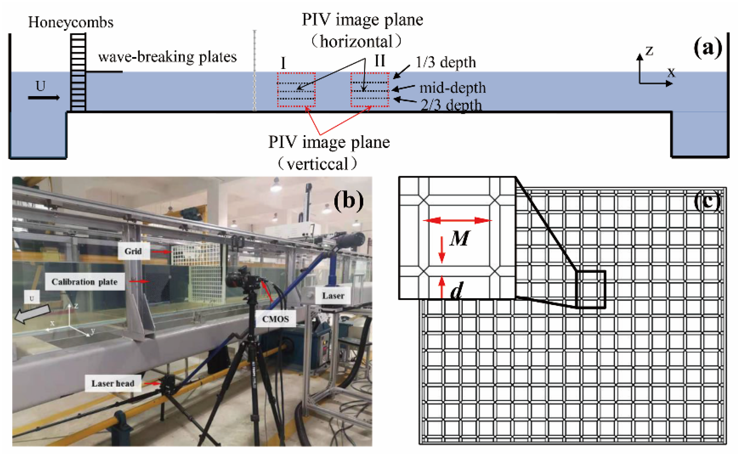
Experiments were performed in the open-recirculate water channel of the Coastal Laboratory in the Ocean College of Zhejiang University. The water channel has a length, width, and height of 25, 0.6, 0.5 m respectively, and its glass walls provide optical access from the side and bottom. Schematics of the experimental setup and test rig with PIV equipment are shown in Figure 1a,b. As previous studies with similar test condition and flow regime show [19], the flow in main flow region around mid-depth of the channel far downstream of the obstacle is generally homogeneous in water depth direction. In this work, honeycombs and wave-breaking plates were installed at the tunnel entrance far enough (about 10 m) upstream of the test section to ensure a vertically uniform base flow away from boundaries without grid more certainly [25,26]. The test flow condition was fixed, where the water depth was 0.3 m with a free flow velocity (U∞) of 0.36 m/s. The Froude number was 0.21. Hence, the free surface has less impact on base flow and there is no hydraulic jump after grid. The channel was set with no slope to make the water surface horizontal upstream of the grid. The average stream-wise turbulence intensity u′/U of the free stream (base flow) was 2.2% and the isotropic degree defined by u′/v′ was 1.38, a value greater than unity and 1.2 for isotropic flow in a straight chamber [27]. Then, the stream penetrated a mono-planar grid placed perpendicular to the flow. The grid used in the present work was made from photopolymer via additive manufacturing and consisted of cylinder rods with surfaces carefully polished to the same roughness level. Figure 1c depicts the schematic of grid geometry, where the mesh spacing M is 33.6 mm and rod diameter d is 6.3 mm. The solidity σ of this grid is defined by (d/M)/(2−d/M) is 0.34. Previous research with similar grid dimensions included those conducted by Cardesa-Duenas et al. [17], Murzyn and Bélorgey [18,19] in an open water channel. For the current case, the cross-stream span and vertical height of the grid immersed in water were around 18 M and 9 M, respectively. The Reynolds number based on mesh spacing ReM = U∞M/ν is 11,880.
The measurement sections of PIV at intermediate downstream distances are shown as the dotted-line frames in Figure 1a. The origin of x direction is at the grid, the origins of y and z direction are at mid-span of channel and mid-depth of the water, respectively. This system of axes is more convenient to distinguish the sphere of influence from different factors (free surface and channel bottom) on the main flow region. The two groups (I and II) of horizontal and vertical measurement sections were, respectively, centered at x/M = 8 and x/M = 18 in the stream-wise direction. Among them, the horizontal measurement sections centered at mid-span were located at 1/3 depth, mid-depth and 2/3 depth of the water to study the flow distribution in the main flow region. As the channel bottom made of glass was different from a rough bottom in an actual river way, the TBL itself and the flow distribution in this zone were not the topic of this paper. Therefore, the vertical measurement sections were located at mid-span and centered at z/M = 0.5 to cover the main flow stream and the zone near the water surface. The lower edge of the vertical field of view (FOV) was roughly 1 M from the bottom of channel.
2.2. Measurement Technique
Flow fields were measured using a two-dimensional (2D) two-component (2C) PIV system (Davis 8.2.3, LaVision GmbH, Goettingen, Germany). Tracer particles of the flow were hollow glass spheres (110P8) with the density of 1.1 g/cm3 and diameter of 8 μm. A light sheet with a wavelength of 532 nm and equivalent output energy of 100 mJ pulse−1 was launched using an Neodymium-doped Yttrium Aluminum Garnet (Nd:YAG) laser (Litron LPY series, LaVision GmbH, Goettingen, Germany) in a continuous trigger model to illuminate the flow field. To avoid out–of–plane particle loss as far as possible [17], the thickness of light sheet was 2 mm. Particle images were recorded by a Complementary Metal-Oxide-Semiconductor (CMOS) camera (Imager MX 4M, LaVision GmbH, Goettingen, Germany) with 2048 × 2048 pixel resolution at a sampling rate of 60 Hz. The placement of the laser head and camera when shooting the vertical section is shown in Figure 1b and transposition was made for horizontal measurement. The camera was triggered in a double-shutter model by a Programmable Timing Unit (PTU). Considering the intense fluctuation near the grid which would lead to high possibility of correlation loss due to out-of-plane particle motion, the time interval between frame pairs was changed appropriately to guarantee a high, valid rate of vector field at each station. Because a relative thick light sheet has been chosen, this time interval was controlled to capture majority of turbulent particles in the sphere of laser beam. Finally, the time intervals were set in the range from 2.5 ms for flow fields in group I to 3.2 ms for group II, roughly corresponding to mean particle displacement of 7 pixels to 9 pixels, respectively. The FOV covered a flow area of 264 mm × 264 mm, which spanned across a distance of 7.6 M × 7.6 M. Sampling time was 61 s (about three triple-length of previous PIV test setting by Cardesa–Duenas et al. [17]) and a series of 4000 flow images was recorded at each station to reduce random errors. Raw PIV images were first preprocessed by sliding the background filter to reduce intensity fluctuation. Instantaneous velocity vector fields were then calculated using the cross-correlation algorithm based on fast Fourier transform [28] in a multi-passing decreasing size procedure. Sizes of final interrogation windows were 32 × 32 pixels with 50% overlap, yielding 126 × 126 vectors with a spatial resolution of 2.1 mm × 2.1 mm. The valid rates of output vector fields at each station were more than 99%. For more details of post-processing, readers can be referred to Gao et al. [26]. One thing worth emphasizing is that the present resolution was not fine enough to resolve the micro-scale parameters of turbulence, while this work only focuses on the macro-scale flow features as shown in the next section and their spatial variation.
3. Data Analysis
3.1. Turbulence Intensity
In a turbulent flow, the local mean velocities U, V and W are time-average x, y, z components of instantaneous velocities U(t), V(t) and W(t) at each pixel point, u, v and w are fluctuating velocities. The fluctuating magnitudes are defined by the mean square roots of three components as below:
Hence, the turbulence intensities are calculated by u′/U, v′/U and w′/U. For current PIV data, the invalid rate for missing and exceptional vectors in each image is less than 1% by outlier detection. These points are removed to avoid bias for turbulence intensities and spectra [29]. The 95% confidence interval is used for uncertainty analysis. That is to say, the true value of statistics θn is within the interval , where is the sampling variance of θn and N is 4000. The level of relative uncertainty for mean velocity is 2.5% and fluctuating velocity is 4.3%.
3.2. Space-Time Correlation
For ideal homogeneous and isotropic turbulence, the canonical Taylor hypothesis relates the spatial patterns with temporal ones by a fixed convection velocity [30]. The space-time correlations shrink into a diagonal line as this hypothesis is only a first-order approximation of space-time correlation [31]. The normalized space-time correlation coefficient of stream-wise velocity is defined as follows:
where r is stream-wise separation and τ is time delay, x and t are original stream-wise position and time moment, respectively. The symbol ‘<>’ represents operation of ensemble average. The elliptic approximate model with second-order precision for space-time iso-correlation contours proposed by He and Zhang [24] is given as:
where rE varies with the value of correlation coefficient. The two characteristic parameters in this model are convection velocity Uc and sweep velocity Vs, which can be calculated from measured space-time correlation function as below:
where rmax and τmax maximize the correlation coefficient for every given τ and r, respectively. Then the ratios rmax/τ and τmax/r are estimated by linear fitting of the slopes [20,32].
3.3. Integral Scales
When fluctuating velocities in FOV are available, the spatial correlation function, which was first explored by Taylor [30], Von Karman and Howarth [33] to formulate the scale and energy transfer of turbulence, can be calculated as follows:
where f(r) and g(r) are termed as longitudinal and lateral correlation functions, respectively. The integral scales are defined as the maximum connection or correlation distance between two points in the flow field [34]:
where upper limit rmax is determined by the stream-wise separation for the first zero crossing [35] of f(r) or g(r). This length scale is also corresponding to the scale of prevailing flow structure containing the most turbulent energy.
4. Results and Discussion
4.1. The Downstream Flow Evolution in Main Flow Region
The first part focuses on the downstream evolution of mean velocity, fluctuating velocities, space-time correlation functions and scales of energetic prevailing flow structures in horizontal PIV sections.
4.1.1. Mean Flow
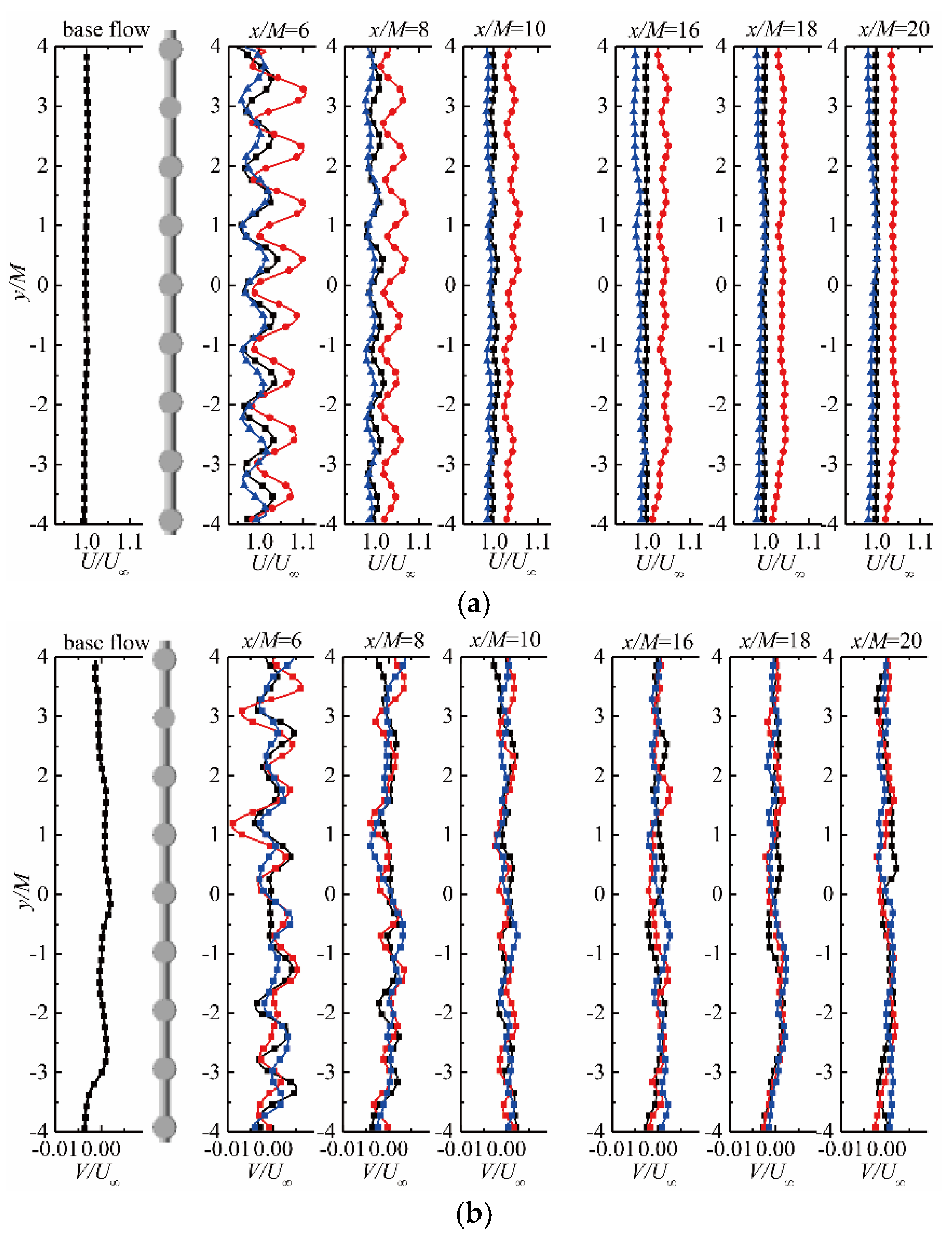
Figure 2 shows the evolution of mean velocity distributions in horizontal direction as a function of downstream location x/M. Because a 2D 2C PIV system was used in the current work, only stream-wise and transverse components were acquired on horizontal sections. To reveal the disturbing effect of grid, the velocity distributions of base flow upstream the grid is presented as a benchmark and the mean velocity is normalized by U∞ to show the changes relative to free stream velocity. As the main flow region of upstream flow was well rectified [25,26], we only recorded the flow field without grid at mid-depth of channel to demonstrate the characteristic of base flow here. The transverse uniformity of U in base flow demonstrates that upstream flow across the FOV around the mid-span is nearly unaffected by the boundary layer of channel side wall. Only slight decreases for V are observed at the edge of FOV, which is due to the extrusion of main flow by side walls. The spatial averaged value of V/U∞ tends to zero and the magnitudes of V are small enough. All of these prove the fine effect of rectifying the device, again.
The mean flow distributions at intermediate distance indicate strong dependence on x/M. At x/M = 6, both U and V exhibit spatial fluctuation corresponding to grid structure. At mid-depth of the water, the mean velocity U attains its peak downstream the mid-distance of two grid rods whereas U is low along the centerline of rod wake. At 1/3 depth, the flow is affected by water surface waviness close to the grid more intensively as the peak-to-peak separation is smaller. For transverse velocity V, adjacent peaks and valleys tend to distribute on two sides of the grid rod, with the same distribution as that at x/M = 0.5 [17]. This is attributed to the counter rotating vortexes shedding from the rods. Hence the turbulence wake vortexes are still not fully emerged at x/M = 6. The different distribution trend for V on each depth indicates the three-dimensional nature of flow.
As the flow develops, both the spatial fluctuation of U and V diminish. To the downstream distance of x/M = 20, the stream-wise flow below mid-depth basically reverts to the uniform level in horizontal direction as base flow. While for U close to water surface and transverse velocity V, there is still a residual inhomogeneous component.
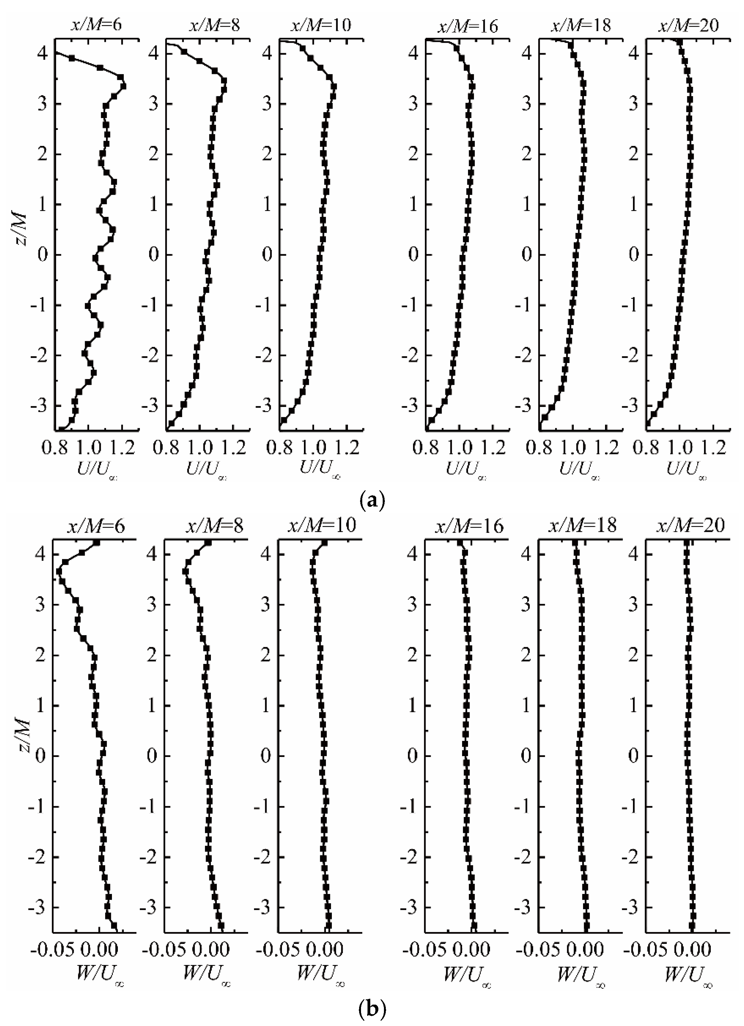
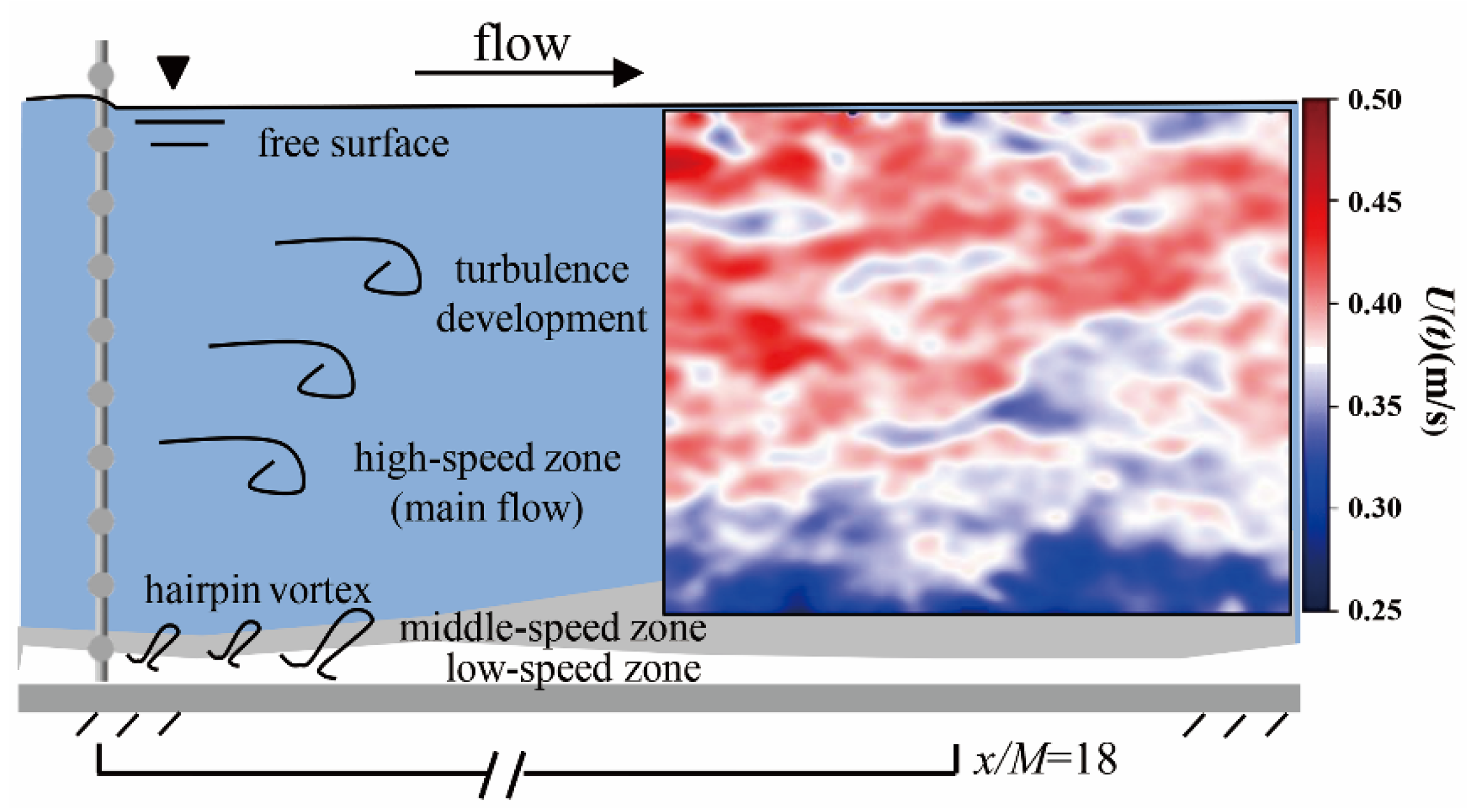
Figure 3 describes the evolution of mean velocity in vertical measurement sections at the mid-span of channel. The positive of W directs upward and the free surface locates at z/M = 4.3. From the distribution in Figure 3a, one can distinguish the influence of upper free surface. The free surface restricts stream-wise flow close to the grid as U decreases rapidly at x/M = 6, which is also revealed by Murzyn and Bélorgey [19]. However, flow through the grid spacing proximate to free surface is accelerated notably. Figure 3b shows apparent downdrafts in this region. When approaching the bottom of the channel, the stream-wise velocity demonstrates a slow trend of decline. For x/M < 8, weak but real upwelling from channel bottom is similar to free-surface turbulence in numerical work by Pan and Banerjee [36] and experimental work by Kumar et al. [37]. In the mid-depth region before x/M = 8, the distribution corresponding to the wake pattern of the grid structure is still observed. As the distance increases, the restriction by the free surface weakens while the bottom TBL expands, making U decays even faster. Besides this, there is indeed the influence of flow structure from TBL of the channel bottom on the distribution of U. From the calibration of velocity distribution near the lower edge of FOV, the law of logarithms does not hold. Hence, it can be concluded that the current FOV only covers the outer part of the TBL, namely the middle speed regions and high speed regions as shown in Figure 4. Nevertheless, the velocity distribution in high-speed region is more complicated due to the grid. In vertical direction, the wake generated by grid robs also mixed fully at x/M = 20 and there is no time-averaged convection between different depths. However, in current condition, slight unevenness of downstream flow in the main flow region due to the blockage of the grid still exists until x/M = 20.
4.1.2. Turbulent Flow
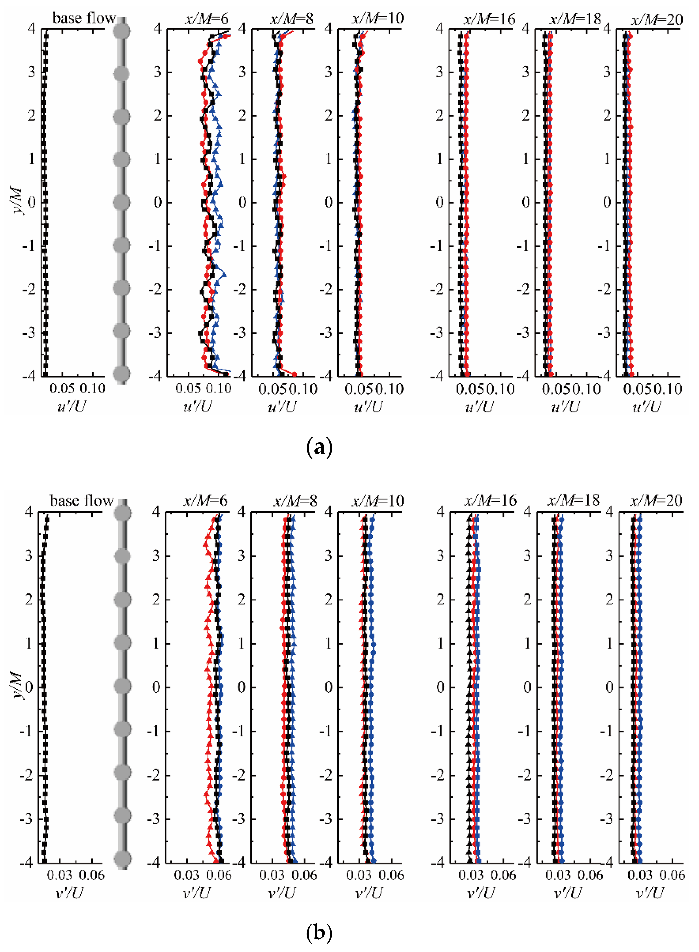
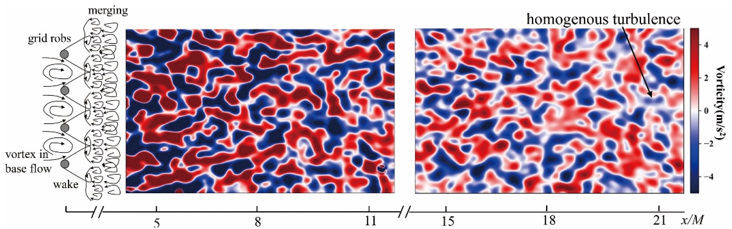
Figure 5 deals with the evolution of stream-wise and transverse turbulence intensity. It shows that the turbulence in base flow is generally homogeneous. Just as with mean velocity, both u′ and v′ near grid are in distribution corresponding to grid structure. At the depth away from free surface, it is noteworthy that the stream-wise intensity downstream the mid-distance of two rods are larger than that along the centerline of rod wake. This distribution is diametrically opposed to the measured results close to the grid at x/M = 0.5 [17]. The cause can be analyzed from the wake pattern depicted in Figure 6. The wakes from adjacent rods converge within the first few mesh distances downstream of the grid and form the initially mixed flow which is the actual inception of downstream homogenous turbulence. In this condition, the mixtures of wakes happening at the downstream location of grid spacing enhance the stream-wise fluctuations here. Meanwhile, the vortexes from base flow pass through the spacing and also contribute to the high intensity here. The same intensity distribution can be seen in the near wake flow of a cylinder–pair [39]. This formation mechanism for grid-generated turbulence is distinguished from that reflected by smoke wires [40], which is mostly due to the different Reynold number and base flow regime. Another side effect of this mixture is more uniform distribution of transverse fluctuation than the stream-wise one due to the counteraction of counter-rotating vortex pairs. However, the distribution of fluctuating intensity at 1/3 depth is random because of the disturbance at the unstable free surface.
Unlike the mean velocity, fluctuating flow at x/M = 20 become comparatively uniform in the horizontal direction and the intensity magnitude is improved by 30% compared to base flow. When calculating the intensity ratio u′/v′, the final values are 1.24, 1.32 and 1.27 at 1/3 depth, mid-depth and 2/3 depth, respectively. From this point of view, the turbulence generated by this grid is homogenous across the span of channel but not completely isotropic.
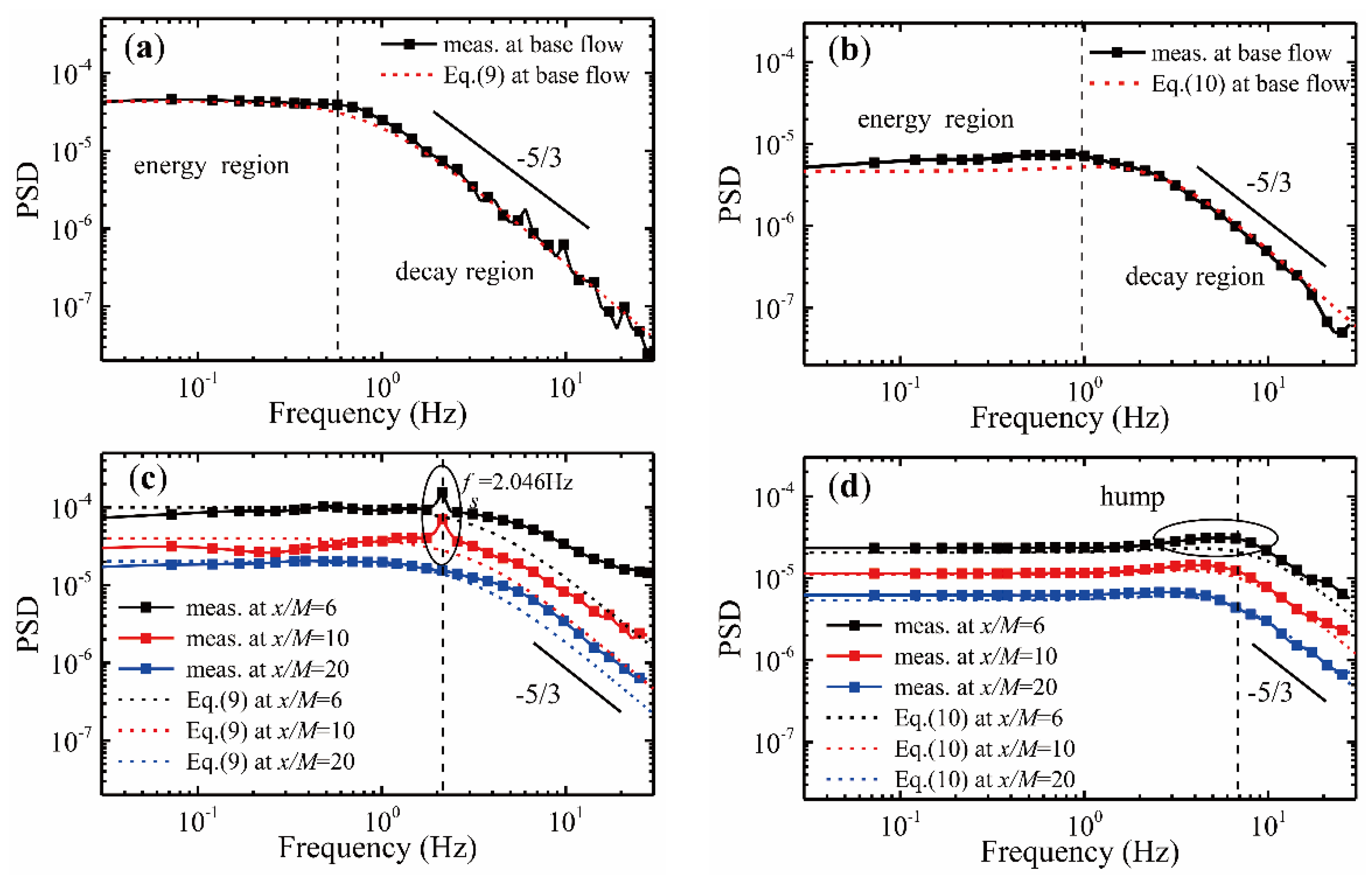
Figure 7 presents the power spectral density (PSD) of fluctuating velocity measured in low-frequency range. To compare with the spectrum of homogeneous isotropic turbulent flow, the following theoretical spectra [35] are also plotted:
As seen, the ranges of energy regions in spectra downstream the grid extend and the magnitude of fluctuating within decay region increases compared with that of base flow. These two changes reveal the decreased scale and enhanced turbulence intensity of flow downstream the grid.
At positions close to grid (x/M = 6, 10), the turbulence is underdeveloped hence the spectrum of u here show a peak fluctuation at fs = 2.046 Hz corresponding to a Strouhal number (Sr = fsd/U∞) of 0.036 based on rod diameter. Farther downstream, the characteristic frequency becomes imperceptible as the wakes merge fully and the magnitudes in whole frequency range decline because the turbulence decays. The decay of turbulence can also be revealed from the declined magnitude of vorticity in Figure 6. In general, the configurations of stream-wise spectra downstream the grid approach to the theoretical spectra but the deviation is still subsistent as turbulence is far from isotropic even at x/M = 20.
For transverse fluctuation, there appear upraised broadband humps of the spectra between energy and decay regions, which are also reflected in theoretical spectra. An identical trend for u and v in the open channel is that the spectra get close to theoretical curves with increased distance and the −5/3 law in decay region become more apparent. Last but not least, the reduced ranges of energy regions with distance for both components reflect the enlarged scales of energy-containing motions as the turbulence develop downstream, which will be also shown from the evolution of integral scale in the next section.
4.1.3. Space-Time Correlation and Integral Scale
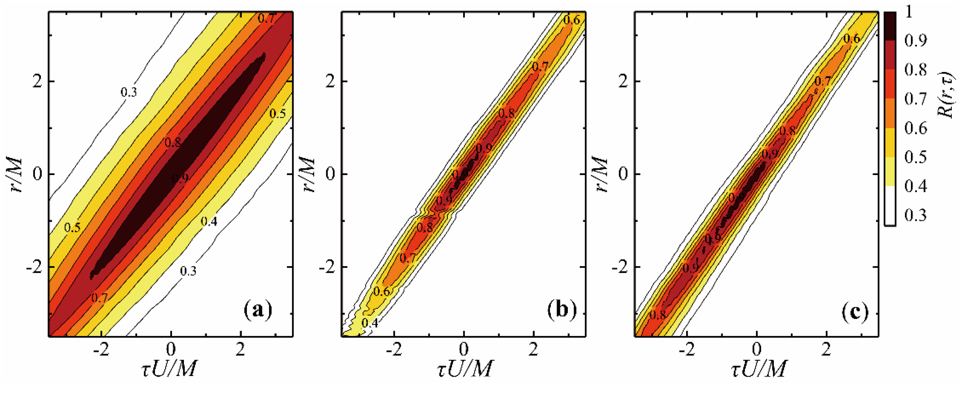
Not only is the fluctuating velocity enhanced by the grid, but also the spatial and temporal flow structures are changed. The normalized space-time correlations of u calculated by Equation (2) at various downstream locations are depicted in Figure 8 along with that of base flow. Actually, the coefficients on the abscissa axis here represent Eulerian-time correlation function and coefficients on the ordinate axis show the longitudinal correlation function as the first quantity in Equation (5). In a physical sense, these correlations are quantitative metrics for prevailing coherent structures or motions in the flow.
As can be seen, all the diagrams reveal a universal distribution wherein the magnitude of correlation decreases with increasing r and τ due to the decorrelation among small-scale motions. However, the low but not zero levels of flow correlation for large space separation and time delay demonstrate the long developing distance and lifetime of coherent structures. The overall shapes are in accord with the results of turbulent shear flow in the boundary layer [20,32]. The iso-contours of space-time correlations for grid-generated flow are flattened compared to that of base flow. As distance increases, the space-time correlation contours expand slightly because the coherent structures generated by grid stretch. Here the convection velocities represented by the slope of diagonal ridge are 1.0 U for base flow, 1.14 U at x/M = 8 and 1.1 U at x/M = 18. This demonstrates the acceleration of the large eddy structure relative to local mean flow at mid-depth.
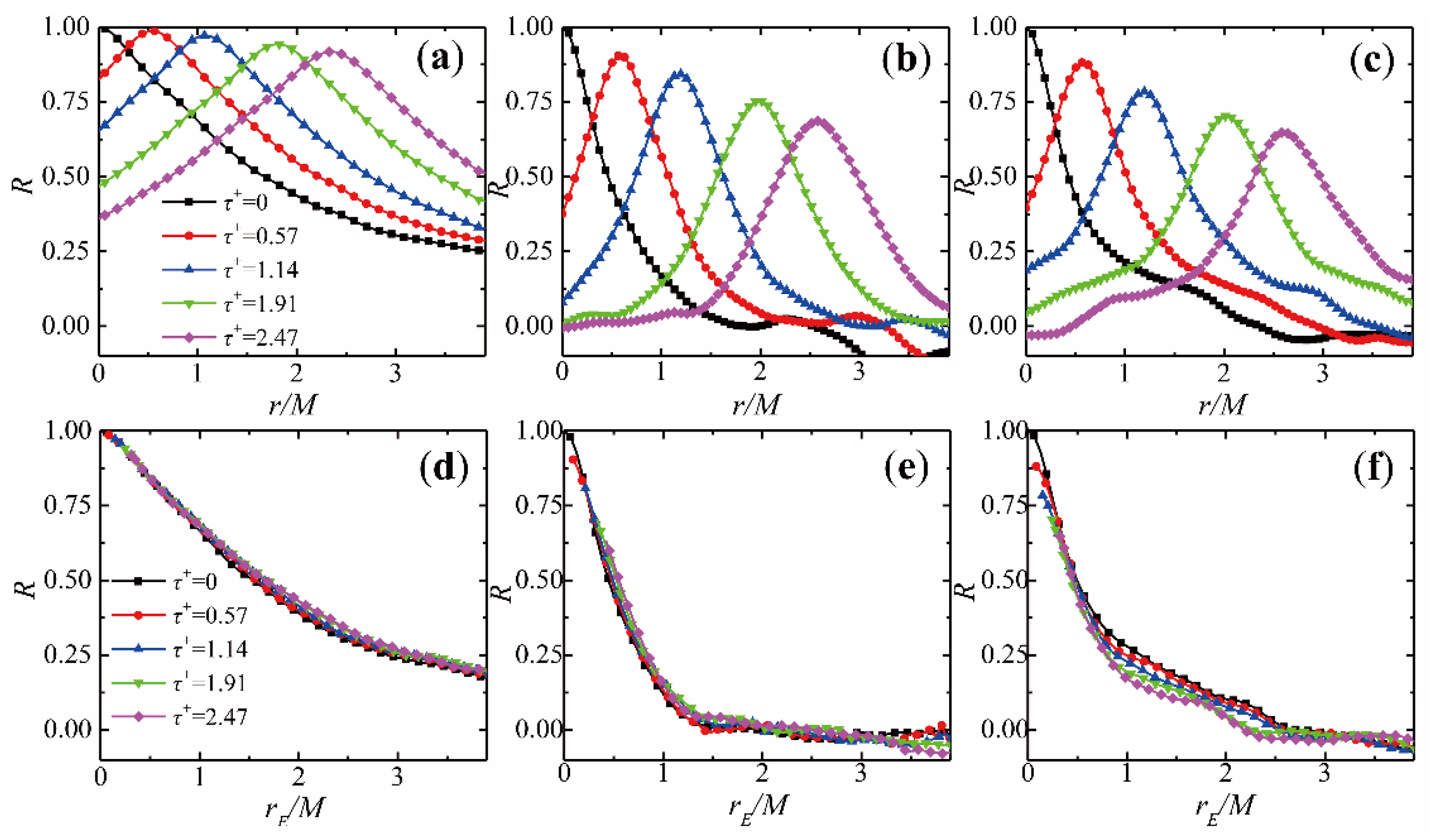
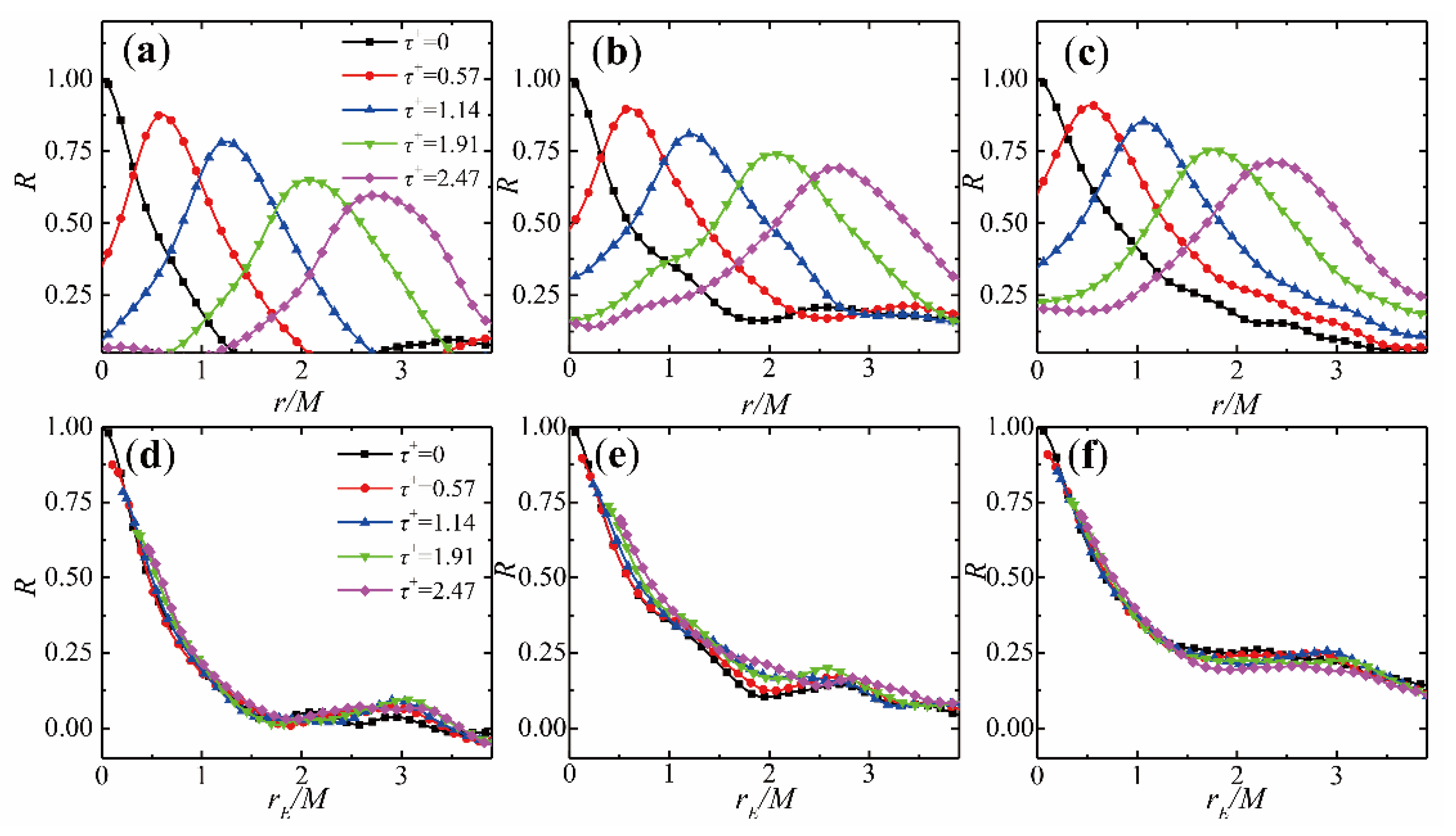
As Wallace [41] put it, the contours of constant correlation for grid flow are elliptical. To validate the elliptic approximate model of Equation (3) for our data in the open channel, the correlation coefficients downstream the grid are displayed as the function of separations for several time delays, as well as the elliptic normalized correlation curves in Figure 9. Correlation curves with non-zero delay present initial increases and then decrease as the temporal autocorrelation is applied. The elliptic model holds well for base flow and location near the grid (x/M = 8) because the curves nearly collapse to a universal form. Although the normalized curves at x/M = 18 do not fit the model that well, the disagreements mainly occur at intermediate separation and this can be probably attributed to the prominent decay of coherent structure intensity far downstream of the grid. In general, the elliptic model is effective for the flow at mid-depth.
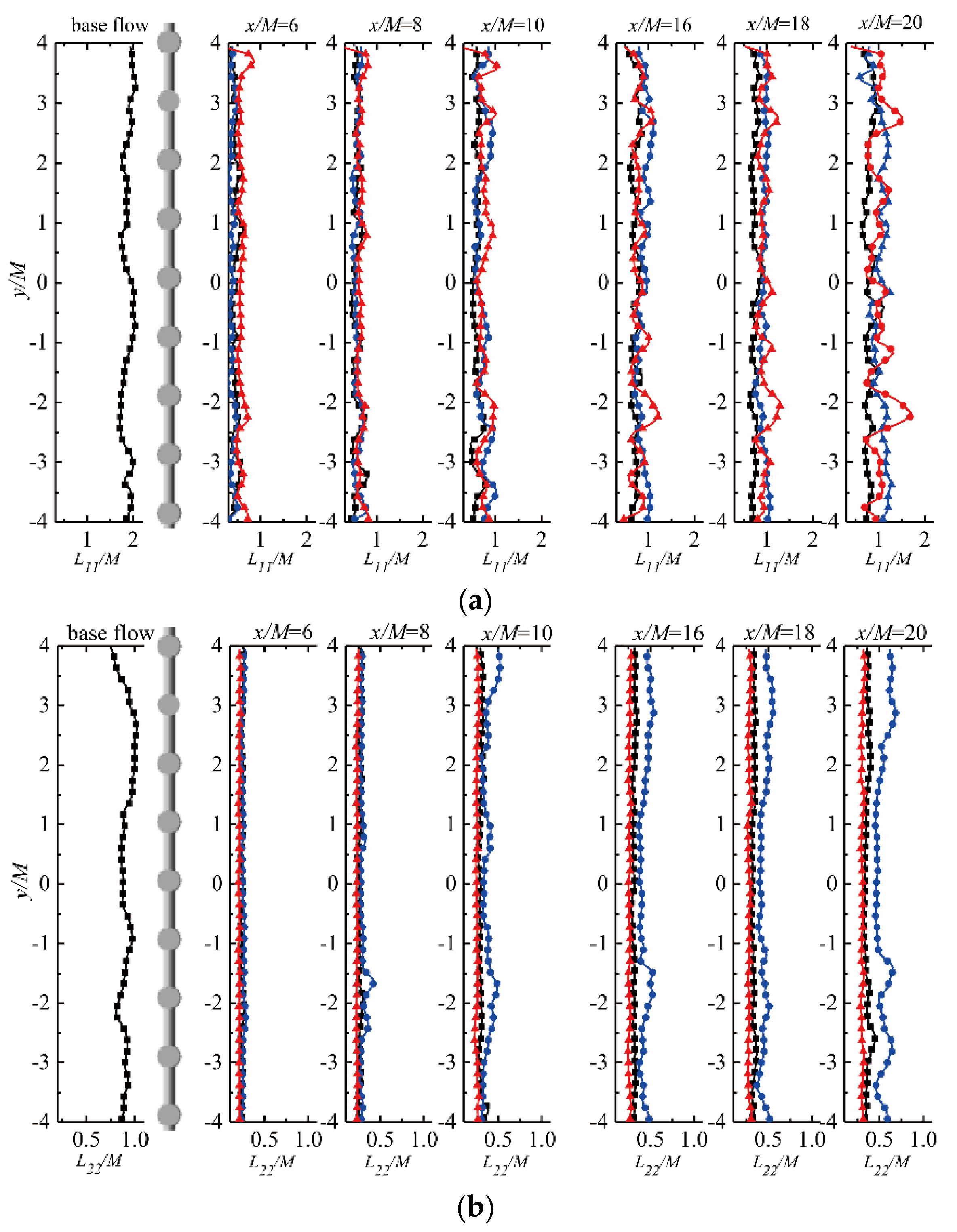
Figure 10 shows the evolution of horizontal distributions for longitudinal and lateral integral scales. The length scales are normalized by M. Unlike the fluctuation intensity, the integral scales in two directions experience a growing tendency as turbulence develops downstream. At x/M = 20, L11/M reaches an averaged value of 1, which is the same as the result of Cadiergue [42]. This is greater than some previous studies [19,43]. The reason is attributed to the considerable length scales from the base flow and the different measurement technique for integral scales (most previous results are calculated based on Taylor hypothesis from temporal data).
Another trend worth mentioning is that L11/M at 1/3 depth become more scattered in the horizontal direction as the prevailing flow structures stretch downstream. Here, the stream-wise coherent structures maintain over a long distance because the distributions from x/M = 10 to 20 share similar configuration and only differ in magnitude while transverse scales at this depth distribute uniformly. It can be concluded that the free surface impacts the stream-wise flow structures more intensively. Compared to the base flow, the homogeneity of L22/M at the upper part of the main flow is improved by the grid but the change for L11/M is negligible. At 2/3 depth, both the distributions of L11/M and L22/M become increasingly uneven as distance increases because of the development of coherent structures in the bottom TBL.
4.2. The Flow Diversity in Depth Direction
As mentioned previously, the upper and bottom regions of the main flow are influenced by the free surface and outer part of TBL at intermediate downstream distance. Although, the TBL itself is not the focus topic of this paper due to the deviation of the smooth bottom in the current channel from an actual rough river bed. This does not prevent us from investigating the influence of disturbance from the TBL on the grid turbulence in main flow region. For fear that some potential common law would be left out, the effects of these two factors on turbulence flow, energetic flow structures (depicted by integral scales) and space-time correlations are reflected and discussed based on PIV data of vertical sections.
4.2.1. Turbulent Flow
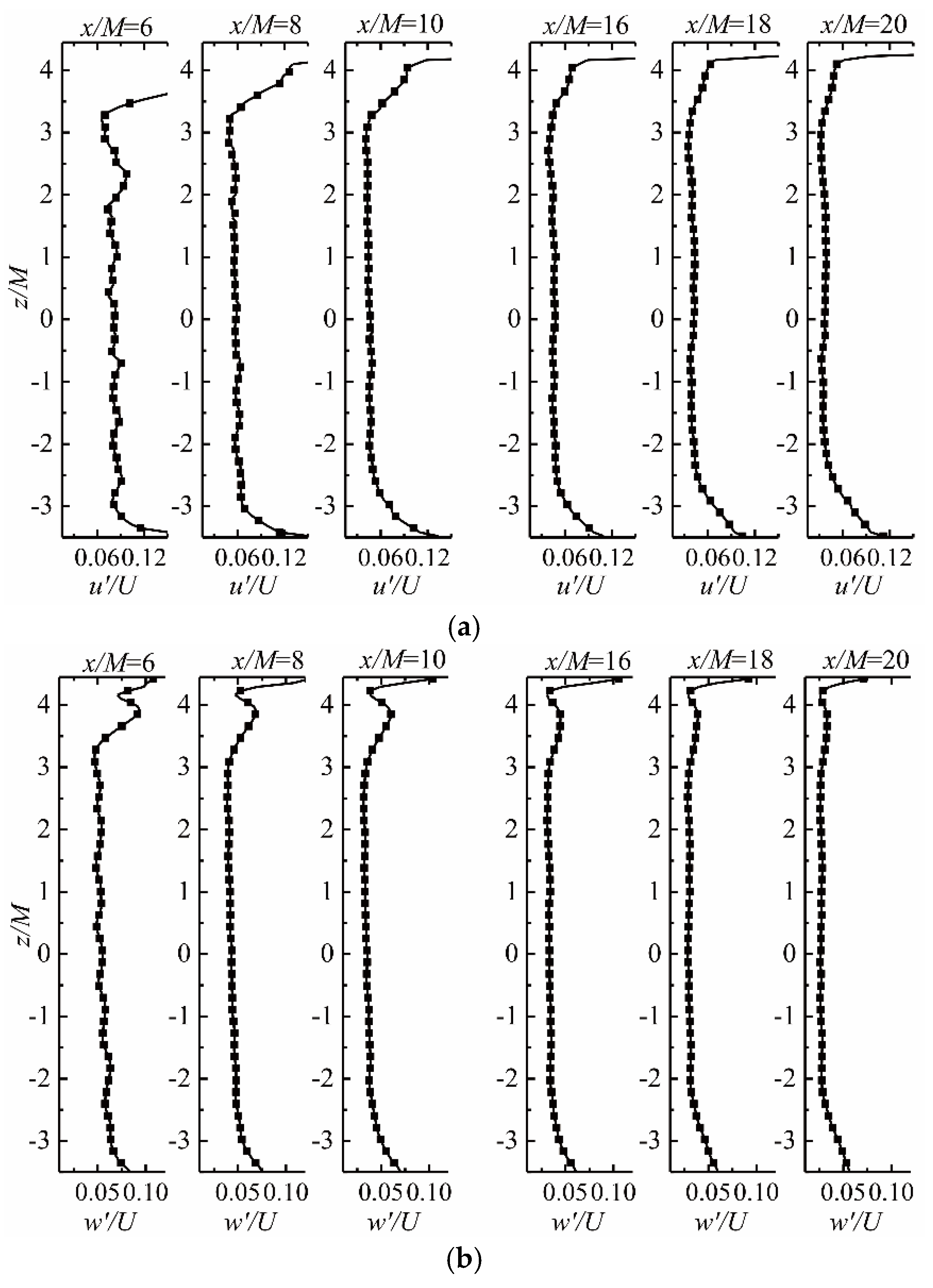
The distributions of stream-wise and vertical fluctuating intensity in the water depth direction are plotted in Figure 11. The distribution configuration of u′ is contrary to mean velocity U in Figure 3, namely the turbulence intensities are enhanced near the free surface and channel bottom. The former is due to the disturbance of interface instability and the latter is due to the bursts arising from TBL. This trend is also observed in the measurement by Murzyn and Bélorgey [19], who reported that the frame of the grid caused a strong turbulence area near the channel bed while the grid used in this work has a flat frame with little disturbance to the downstream flow, hence the effect of TBL is dominant here. The vertical distribution of w′ is the same as u′. However, w′ shows a persistent oscillation around z/M = 4 caused by the downdrafts between the water surface and adjacent grid rod. In this case, the influence of interface diminishes as the water surface restores calm downstream because the areas where intensity shrinks reduce. The TBL extends its influence range on the main flow but the gradients of fluctuating flow in the middle-speed zone decrease. In general, vertical homogenous turbulence is achieved at x/M = 20 for main flow around mid-depth.
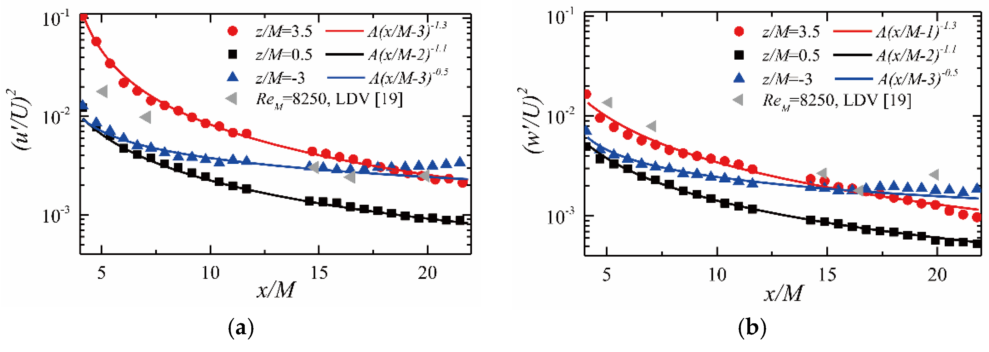
To reveal the impact of the interface and bottom TBL on turbulence decay, Figure 12 concerns the stream-wise evolution of intensity components at water depths of z/M = 3.5, 0.5 and –3, representing the regions under the influence of different factors. As the horizontal distributions of velocity and intensity show that the vortex in grid wakes merge after a downstream distance at x/M = 10 for the region far from the free surface, the fluctuation intensities in current flow are asymptotic to the power-law decay in homogenous turbulence described by Batchelor and Townsend [12].
where x0 is a virtual origin position. The fitting for current data at various depths leads to variation for the decay exponent b and coefficient A, which confirm the acknowledged dependence of decay behavior for grid turbulence on initial conditions and flow regime [44]. At z/M = 3.5 and 0.5, the decay exponents change slightly from −1.3 to −1.1, around a deduced value of −1.2 from the conservation law with finite initial energy [45]. This reflects the fact that the turbulence kinetic energies generated by the grid at the superficial layer are partly consumed by the motion like downdrafts near the water surface. Therefore, the turbulence here decays more rapidly than that at mid-depth. As it becomes closed to the grid (x/M < 5), the prominent fluctuation of water surface and downdrafts contribute to the energy to a great extent, making the slope here larger than the same downstream position at z/M = 0.5. At z/M = −3, a smaller decay rate of −0.5 is observed, which is mainly attributed to the import of energy produced from the bottom TBL to the grid-generated turbulence. The boundary layer acquires energy from the main flow, resulting in the reduction of mean flow velocity in Figure 3, but enhances the fluctuating and decelerates the turbulence decay for the bottom part of grid turbulence. For the points around x/M = 20, there is even a slight lift for both u′ and v′ caused by the sustained energy supplement from the burst and developing hairpin vortex in the expanded TBL. The magnitude of turbulence intensities at a region near the water surface is close to the previous measurements in the open channel [19]. Although the turbulence magnitude at mid-depth (x/M = 0.5) is lower than this result, the decay rate is in good agreement at 5 < x/M < 21. It’s worth noting that the higher level of base flow intensity (less than 4%) in Murzyn and Bélorgey’s work [19] would lead to more considerable residual fluctuation downstream the grid than that in our experiment.
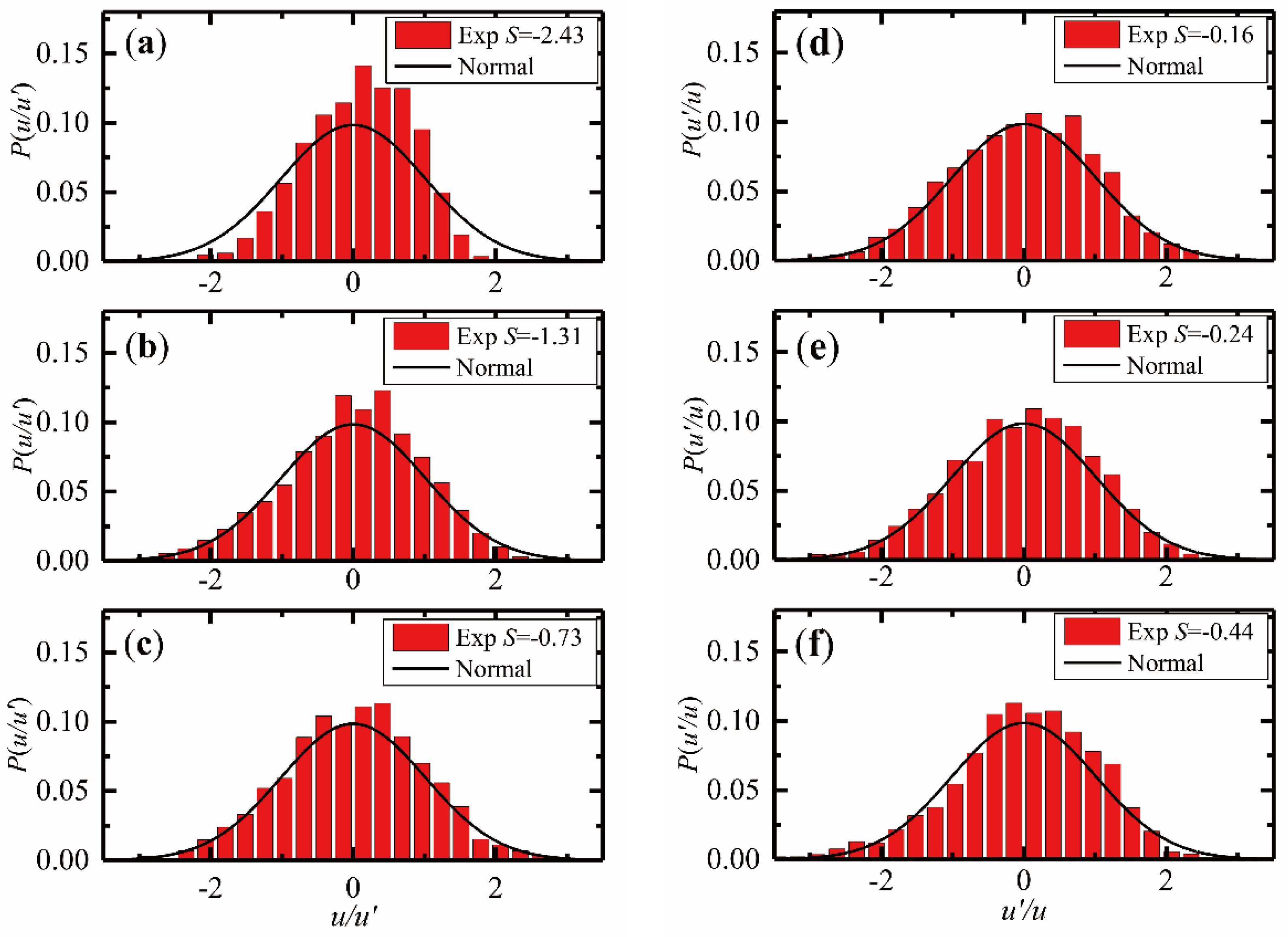
The probability distribution function (PDF) of fluctuating velocity in fully developed homogeneous isotropic turbulence should be close to the normal distribution [46]. The PDFs of stream-wise components at x/M = 6 and x/M = 20 for various vertical locations in current experiment (Exp) are compared with the normal distribution in Figure 13. The skewness (S) of fluctuating velocity is also calculated to evaluate the deviation from the normal distribution. Globally, the skewness of PDF here is negative, that is to say, the grid-generated turbulence in the open channel at an intermediate distance is different from the pure decaying turbulence, of which the skewness is generally positive due to flux of turbulence kinetic energy [47]. The main explanation for this is that the water surface disturbance and TBL development contribute to the production of new turbulence into the main flow. At x/M = 6, the closer it becomes to the free surface, the greater the fluctuations are generated from the motions of the water surface. Hence, it deviates to normal distribution much more. However, at a relatively far downstream location of x/M = 20, an opposite trend in the vertical direction appears because the interface oscillations calm down but the bottom TBL expands with downstream distance increasing.
4.2.2. Integral Scale
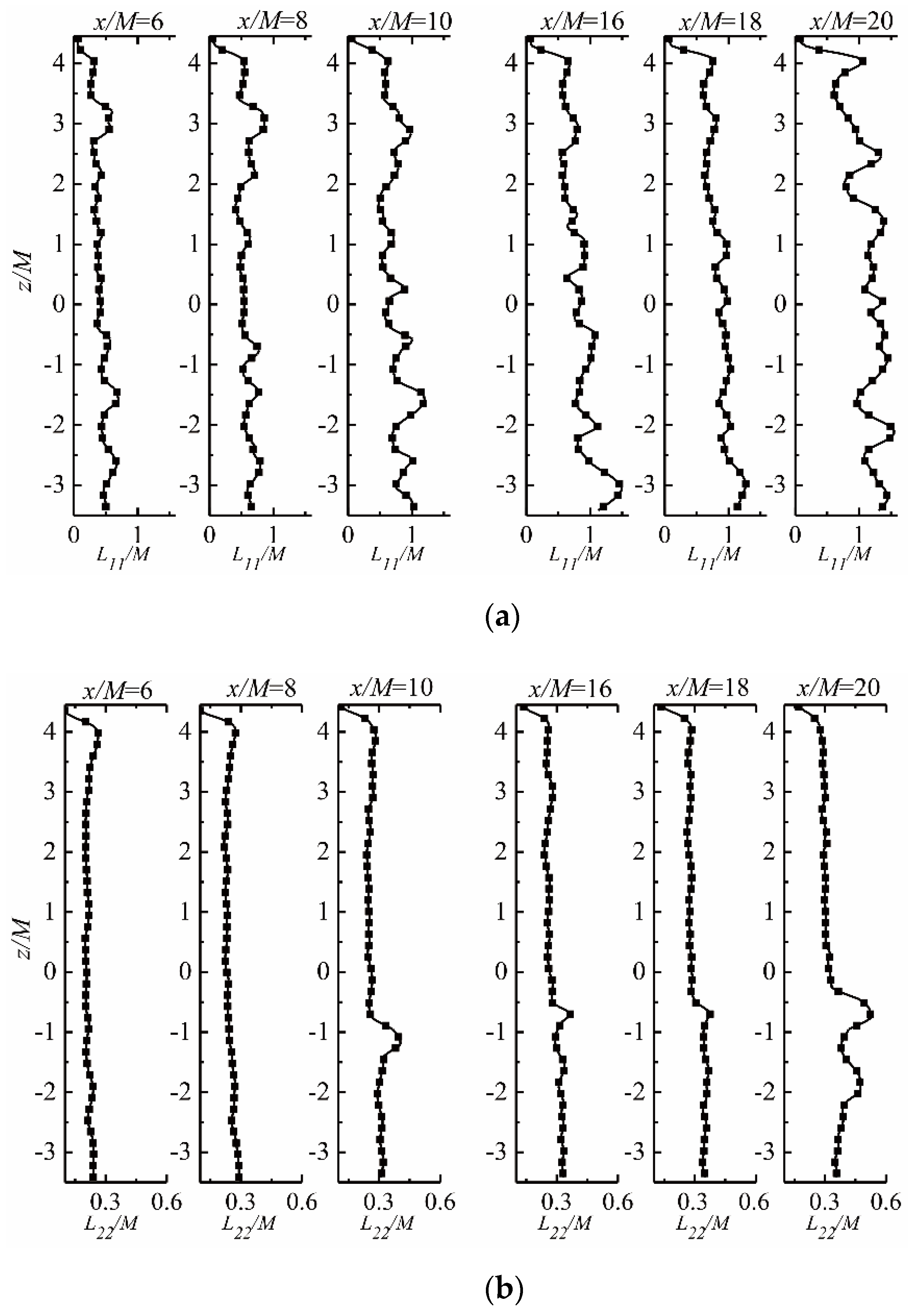
According to the comparison in Figure 9, the grid of current scale breaks the flow structures in base flow and generates new coherent motions and turbulence downstream. This section first deals with the depth diversity in the distribution of integral scale, as shown in Figure 14. Generally speaking, the longitudinal scales show more scattered distribution corresponding to the grid structure than transverse scales, especially at a location far from the free surface. This indicates that the stretch of the vortex in stream-wise direction has a certain memory effect on its initial state. The inhomogeneity of the integral scales enhances as the turbulence develops for different water depths. However, the vertical diffusion is uniform for the wake-mixed turbulence, remembering that L22 here represents the correlation in the vertical direction.
The current FOV spans a vertical range from outer part of TBL to a place adjoining the free surface. The rapid decrease for the calculated scales at the top of the FOV indicates that the large coherent structure is unable to be maintained near the interface. As the depth increases, the longitudinal scales corresponding to the grid cell adjacent to surface show a rising trend. It is necessary to point out that the scale increment here is not as notable as the LDV measured results [19]. Considering the high intensity near the surface in Figure 10, one of reasons for the deviation may come from the employment of the Taylor hypothesis when calculating the macro scales using u′ in previous research. The different flow regime in two experiments is also another possible source. For the region near the channel bottom, the longitudinal integral scales here are higher than mid-depth due to the expanded flow structure in bottom TBL. Meanwhile, there appear obvious humps in the distribution of L22 as distance increases. This is mostly due to the hairpin vortex incepted from the channel bed as shown in Figure 4. As the flow moves downstream, the vortexes lift and stretch, along with the formation of new hairpin vortexes into vortex packets. Meanwhile, the rapid increment for L11 from x/M =−2 to −3.5 would also be attributed to this.
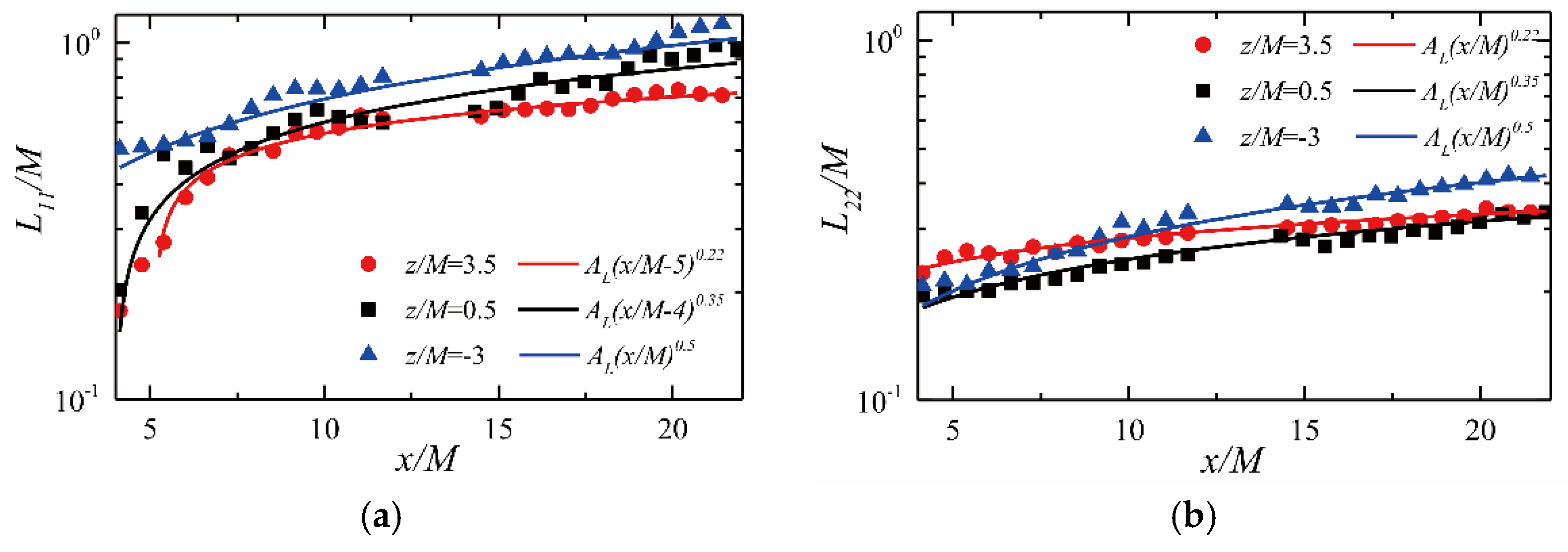
In Figure 15, the quantitative descriptions for the extension of integral scales at various water depths are depicted. A similar power law as Equation (9) for integral scale is fitted for the measured data here. The non-linear shapes for fitting curves at small x/M mean non-zero origin location of x0. Although M/d for the current grid is around 5, the exponent rates for the regions of mid-depth and near surface are smaller than the typical value of Equation (12) [48]. This deviation is mainly due to the residual flow structure from the base flow. The exponent rate becomes larger as depth increases and it is exact 0.5 at z/M = −3. At this stage, it can be concluded that the free surface would suppress the extension of flow structures generated by the grid. The final ratios of L11/L22 at x/M = 20 are 2.2, 2.9 and 2.7 for the three vertical locations here, representing again the anisotropy of the turbulence [49] in the open channel.
4.2.3. Space-Time Correlation
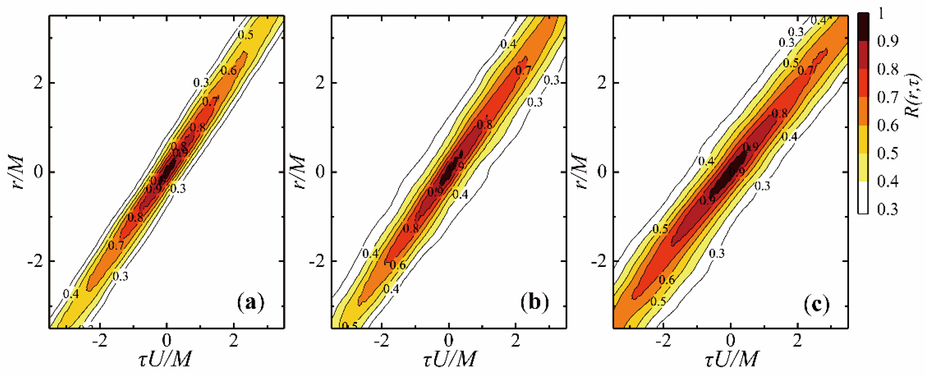
The above discussion suggested that the main flow in various water depths has a different nature due to the upper interface and developed TBL from the channel bottom. From the gradients of vertical velocities in Figure 3, one can deduce that there exist shear motions of different levels for flow near the surface and channel bed. The flow around mid-depth is affected by less shear layer. Figure 16 compares the contours of space–time correlations at different water depths from the vertical sections centered at x/M = 18. It can be seen that, for downstream distance where the turbulence is fully mixed, the shapes of correlation are all approximate to ellipses. The gradually expanding profiles from z/M = 3.5 to −3 are consistent with the increased integral scales in Figure 14.
The spatial correlations at different time delays and verification of the elliptical model for these three locations are described in Figure 17. The normalized curves for z/M = 3.5 and −3 confirm the elliptical model well, while there is still an error for z/M = 0.5 at intermediate separations. When it nears the upper and bottom parts, the shear motions surpass the turbulence decay. Hence the elliptical model would fit well.
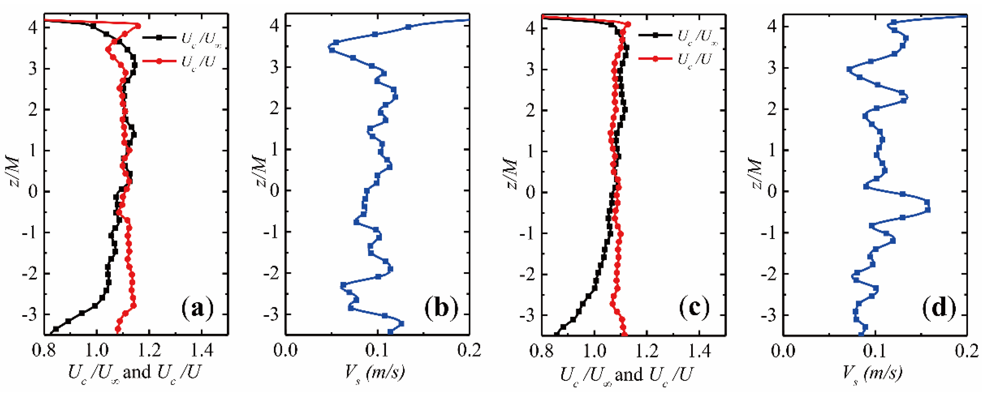
The vertical distribution of convection velocity Uc and sweep velocity Vs for the space-time correlation contours are shown in Figure 18. According to the elliptical model [24], convection velocity Uc determines the slope of preferred orientation of correlation curves and sweep velocity Vs represents the aspect ratio of iso-correlation contours. Thus, the greater the sweep velocity, the more it would deviate from the Taylor hypothesis. In a physical sense, the large-scale eddies in flow carry the small-scale ones at the velocity of Uc and Vs characterizes the distortion of small-scale eddies [24,32].
As can be seen in Figure 18, the convection velocities at x/M = 8 and x/M = 18 are both normalized by free flow velocity U∞ and local mean stream-wise velocity U in Figure 3. The ratios Uc/U∞ are in rapid decay below z/M = −2.5, which shows the deceleration of large-scale eddies in the scope of TBL, the same as was revealed by Wang et al. [20]. In the main flow around mid-depth, Uc rises slowly when it approaches free surface. At z/M = 3 corresponding to the nearest grid cell to the interface, Uc/U∞ reaches a maximum value of 1.1. However, when it nears the free surface, Uc vanishes as the interface suppresses the large-scale motions here, in contrast, the small-scale fluctuation is increased making the sweep velocity undergoes an enhancement, especially at x/M = 8 where the surface is still unstable. The ratios Uc/U show that the convection velocities are generally proportional to local mean velocity, except for the regions where the large-scale motions are confined by free surface. Although, previous experiments [50] on grid turbulence demonstrated that convective velocities are nearly equal to local mean velocities in fully developed regions. According to the theoretical analysis by He and Zhang [24], the departure of Uc/U from unity in this measurement is primarily attributed to the considerable velocity fluctuation and shear rate residuals in the wake generated by grid rods. As the turbulence decays downstream, the ratios Uc/U in the main flow diminish gradually. The non-zero sweep velocity in the water depth direction demonstrates that there indeed exists the random sweeping of small-scale eddies [51,52] here and the small-scale fluctuations do not dissipate much from x/M = 8 to x/M = 18. Another notable thing is the results in this work do not show the expected decline from the outer part of TBL to the main flow region as in the boundary layer of the flat wall [20]. This is necessary due to the existence of small-scale coherent structures from the grid-generated turbulence.
5. Conclusions
The 2D 2C PIV system was used in the present work to investigate the stream-wise evolution and spatial distribution of grid turbulence during its initial period of decay in an open channel. The mean flow velocity, turbulence intensity, integral length scale and correlation function have been estimated on the image sections of different stream-wise locations and water depths. The main contribution of this paper is the presentation of interesting information on the evolution and depth diversity of grid turbulence with free surface. Taking the advantage of PIV technology in recording spatial flow fields synchronously, the detailed and direct measurement on distribution of turbulence characteristics reveal some novel flow phenomena which have not been discovered in previous measurements by LDV. These would help in the design of flow passages after filter or rectifying devices in sediment transport, sewage outfall, coastal platform or other applications. Last but not least, the application scope of an elliptic approximation model is expanded through the verification of the space-time correlation functions at various regions of the channel. The characteristic velocities in this model provide a novel way to represent the motions and fluctuations in channel flow. The main conclusions are derived as follow:
- The uniformity of turbulence intensity and lateral integral scales is improved with increasing distance. Horizontally uniform flow and homogenous turbulence in the main flow region around the mid-depth is achieved after x/M = 10. However, the distribution of longitudinal integral scale becomes more disorganized as the stream-wise coherent structures develop downstream.
- The elliptical model is more applicable for flow regions with larger shear rates (near the water surface and channel bottom) and high turbulence intensity (x/M < 10). The convection velocity of large-scale eddies is generally 10% larger than the local mean velocity in the main flow region. Both the interface and TBL restrict the convection of large-scale eddies. The magnitude of sweep velocity remains almost unchanged in the current downstream range, indicating that the small-scale fluctuation would be maintained for a long period.
- With the setup of the grid, not only is the turbulence intensity enhanced, but the isotropic degree at intermediate downstream distance is also improved compared to base flow. However, according to the intensity ratio, PSD and PDF of fluctuating velocity, the turbulence in an open water channel is not completely isotropic even at x/M = 20.
- The decay of grid turbulence near the surface is accelerated, while the growth rate of prevailing flow structure here is confined to relatively a low value. For the region affected by TBL from the channel bottom, the turbulence decay slows down but the extension rate of integral scale increases.
In addition, one should be careful about the deviation of wall smoothness for a current experimental apparatus from that in an actual channel. It will be understandable if there is discrepancy with the current result when examining the thickness or flow distribution of TBL in some engineering cases. Therefore, further work could be undertaken to investigate the impact of boundary walls with different smoothness on the grid turbulence in water channels.
Author Contributions
Conceptualization, H.Y.; data curation, L.C.; formal analysis, H.Y. and S.Q.; funding acquisition, D.W.; investigation, H.Y.; methodology, H.Y. and Y.G.; project administration, D.W.; resources, D.W. and Y.G.; software, Y.G.; supervision, F.Y.; validation, H.Y., L.C. and S.Q.; visualization, H.Y.; writing—original draft, H.Y.; writing—review and editing, H.Y. and L.C. All authors have read and agreed to the published version of the manuscript.
Funding
This research was funded by National Natural Science Foundation of China, grant number 51839010 and China Postdoctoral Science Foundation, grant number 2020M671702.
Institutional Review Board Statement
Not applicable.
Informed Consent Statement
Not applicable.
Data Availability Statement
The data presented in this study are available on request from the corresponding author. The data are not publicly available due to privacy.
Acknowledgments
The authors greatly appreciate the assistances from Weiyi Chen, Chenwei Guo and Jianyong He for the experiments.
Conflicts of Interest
The authors declare no conflict of interest.
Nomenclature
| A | Decay Coefficient |
| b | Decay Exponent |
| d | Diameter of Grid Rod (mm) |
| f | Frequency (Hz) |
| f(r), g(r) | Spatial Correlation Functions |
| U, V, W | Local Time-Averaged Velocities (m/s) |
| U∞ | Free Stream Velocity (m/s) |
| Vs | Sweep Velocity (m/s) |
| ν | Kinematic Viscosity of Water (m2/s) |
| L11, L22 | Integral Scales (mm) |
| M | Grid Spacing (mm) |
| R | Space Separation (mm) |
| R(r, τ) | Space-Time Correlation Function |
| U(t), V(t),W(t) | Instantaneous Velocities (m/s) |
| u′, v′, w′ | RMS of Fluctuating Velocities (m/s) |
| Uc | Convection Velocity (m/s) |
| x, y, z | spatial Coordinates in Stream-Wise, Transverse and Vertical Directions |
| τ | Time Delay (s) |
References
- Svenson, A.; Allard, A.-S.; Ek, M. Removal of estrogenicity in Swedish municipal sewage treatment plants. Water Res. 2003, 37, 4433–4443. [Google Scholar] [CrossRef]
- Zeier, K.R.; Hills, D.J. Trickle Irrigation Screen Filter Performance as Affected by Sand Size and Concentration. Trans. ASAE 1987, 30, 0735–0739. [Google Scholar] [CrossRef]
- Sumer, B.; Whitehouse, R.J.; Tørum, A. Scour around coastal structures: A summary of recent research. Coast. Eng. 2001, 44, 153–190. [Google Scholar] [CrossRef]
- Fouad, A.; Khaled, A.H. Liquid-phase axial dispersion of turbulent gas–liquid co-current flow through screen-type static mixers. AICHE J. 2017, 63, 1390–1403. [Google Scholar] [CrossRef]
- Robbins, B.E. Water Tunnel Turbulence Measurements behind a Honeycomb. J. Hydronautics 1978, 12, 122–128. [Google Scholar] [CrossRef]
- Sumer, B.M.; Chua, L.H.C.; Cheng, N.-S.; Fredsoe, J. Influence of Turbulence on Bed Load Sediment Transport. J. Hydraul. Eng. 2003, 129, 585–596. [Google Scholar] [CrossRef]
- Cox, D.T.; Kobayashi, N. Identification of intense, intermittent coherent motions under shoaling and breaking waves. J. Geophys. Res. Space Phys. 2000, 105, 14223–14236. [Google Scholar] [CrossRef]
- Panda, J.; Mitra, A.; Joshi, A.; Warrior, H. Experimental and numerical analysis of grid generated turbulence with and without mean strain. Exp. Therm. Fluid Sci. 2018, 98, 594–603. [Google Scholar] [CrossRef] [Green Version]
- Nagata, K.; Saiki, T.; Sakai, Y.; Ito, Y.; Iwano, K. Effects of grid geometry on non-equilibrium dissipation in grid turbulence. Phys. Fluids 2017, 29, 015102. [Google Scholar] [CrossRef]
- Valente, P.C.; Vassilicos, J.C. The decay of turbulence generated by a class of multiscale grids. J. Fluid Mech. 2011, 687, 300–340. [Google Scholar] [CrossRef] [Green Version]
- Comte-Bellot, G.; Corrsin, S. The use of a contraction to improve the isotropy of grid-generated turbulence. J. Fluid Mech. 1966, 25, 657–682. [Google Scholar] [CrossRef]
- Batchelor, G.K.; Townsend, A.A. Decay of isotropic turbulence in the initial period. Proc. R. Soc. London. Ser. A Math. Phys. Sci. 1948, 193, 539–558. [Google Scholar] [CrossRef]
- Jayesh; Warhaft, Z. Probability distribution, conditional dissipation, and transport of passive temperature fluctuations in grid-generated turbulence. Phys. Fluids A Fluid Dyn. 1992, 4, 2292–2307. [Google Scholar] [CrossRef]
- Mazellier, N.; Vassilicos, C. Turbulence without Richardson-Kolmogorov cascade. Phys. Fluids 2009, 22, 331–341. [Google Scholar] [CrossRef] [Green Version]
- Valente, P.C.; Vassilicos, J.C. Dependence of decaying homogeneous isotropic turbulence on inflow conditions. Phys. Lett. A 2012, 376, 510–514. [Google Scholar] [CrossRef] [Green Version]
- Gramespacher, C.; Albiez, H.; Stripf, M.; Bauer, H.-J. The generation of grid turbulence with continuously adjustable intensity and length scales. Exp. Fluids 2019, 60, 85. [Google Scholar] [CrossRef]
- Cardesa, J.I.; Nickels, T.B.; Dawson, J.R. 2D PIV measurements in the near field of grid turbulence using stitched fields from multiple cameras. Exp. Fluids 2012, 52, 1611–1627. [Google Scholar] [CrossRef]
- Murzyn, F.; Bélorgey, M. Wave influence on turbulence length scales in free surface channel flows. Exp. Therm. Fluid Sci. 2005, 29, 179–187. [Google Scholar] [CrossRef]
- Murzyn, F.; Bélorgey, M. Experimental investigation of the grid-generated turbulence features in a free surface flow. Exp. Therm. Fluid Sci. 2005, 29, 925–935. [Google Scholar] [CrossRef]
- Wang, W.; Guan, X.-L.; Jiang, N. TRPIV investigation of space-time correlation in turbulent flows over flat and wavy walls. Acta Mech. Sin. 2014, 30, 468–479. [Google Scholar] [CrossRef]
- Espa, S.; Avallone, G.; Cenedese, A. Decaying grid turbulence experiments in a stratified fluid: Flow measurements and statistics. Stoch. Environ. Res. Risk Assess. 2018, 32, 2325–2336. [Google Scholar] [CrossRef]
- Discetti, S.; Ziskin, I.B.; Astarita, T.; Adrian, R.J.; Prestridge, K. PIV measurements of anisotropy and inhomogeneity in decaying fractal generated turbulence. Fluid Dyn. Res. 2013, 45, 061401. [Google Scholar] [CrossRef]
- Gomes-Fernandes, R.; Ganapathisubramani, B.; Vassilicos, J.C. Particle image velocimetry study of fractal-generated turbulence. J. Fluid Mech. 2012, 711, 306–336. [Google Scholar] [CrossRef]
- He, G.-W.; Zhang, J.-B. Elliptic model for space-time correlations in turbulent shear flows. Phys. Rev. E 2006, 73, 055303. [Google Scholar] [CrossRef] [PubMed] [Green Version]
- Ma, L.; Gao, Y.; Guo, Z.; Wang, L. Experimental investigation on flow past nine cylinders in a square configuration. Fluid Dyn. Res. 2017, 50, 025504. [Google Scholar] [CrossRef]
- Gao, Y.; Liu, C.; Zhao, M.; Wang, L.; Zhu, R. Experimental Investigation on Flow Past Two and Three Side-by-Side Inclined Cylinders. J. Fluids Eng. 2019, 142, 011201. [Google Scholar] [CrossRef]
- Uberoi, M.S. Energy Transfer in Isotropic Turbulence. Phys. Fluids 1963, 6, 1048. [Google Scholar] [CrossRef] [Green Version]
- Keane, R.D.; Adrian, R.J. Optimization of particle image velocimeters. Meas. Sci. Technol. 1989, 2, 1202–1215. [Google Scholar] [CrossRef]
- Srikantaiah, D.V.; Coleman, H.W. Turbulence spectra from individual realization laser velocimetry data. Exp. Fluids 1985, 3, 35–44. [Google Scholar] [CrossRef]
- Taylor, G.I. The Spectrum of Turbulence. Proc. R. Soc. A Math. Phys. Eng. Sci. 1938, 164, 476–490. [Google Scholar] [CrossRef] [Green Version]
- He, G.; Jin, G.; Yang, Y. Space-Time Correlations and Dynamic Coupling in Turbulent Flows. Annu. Rev. Fluid Mech. 2017, 49, 51–70. [Google Scholar] [CrossRef] [Green Version]
- Zhao, X.; He, G.-W. Space-time correlations of fluctuating velocities in turbulent shear flows. Phys. Rev. E 2009, 79, 046316. [Google Scholar] [CrossRef] [PubMed] [Green Version]
- Von De Karman, T.; Howarth, L. On the Statistical Theory of Isotropic Turbulence. Proc. R. Soc. Lond. Ser. A Math. Phys. Sci. 1938, 164, 192–215. [Google Scholar] [CrossRef]
- Hinze, J.O. Turbulence; McGraw-Hill Publishing Co.: New York, NY, USA, 1987. [Google Scholar]
- O’Neill, P.L.; Nicolaides, D.; Honnery, D.R.; Soria, J. Autocorrelation functions and the determination of integral length with reference to experimental and numerical data. In Proceedings of the 15th Australasian Fluid Mechanics Conference, Sydney, NSW, Australia, 13–17 December 2004; Volume 1, pp. 1–4. [Google Scholar]
- Pan, Y.; Banerjee, S. A numerical study of free-surface turbulence in channel flow. Phys. Fluids 1995, 7, 1649–1664. [Google Scholar] [CrossRef]
- Kumar, S.; Gupta, R.K.; Banerjee, S. An experimental investigation of the characteristics of free-surface turbulence in channel flow. Phys. Fluids 1998, 10, 437–456. [Google Scholar] [CrossRef]
- Adrian, R.J.; Meinhart, C.D.; Tomkins, C.D. Vortex organization in the outer region of the turbulent boundary layer. J. Fluid Mech. 2000, 422, 1–54. [Google Scholar] [CrossRef] [Green Version]
- Gao, Y.Y.; Wang, X.; Tan, D.S.; Keat, T.S.; Tan, S.K. Particle image velocimetry technique measurements of the near wake behind a cylinder-pair of unequal diameters. Fluid Dyn. Res. 2013, 45, 045504. [Google Scholar] [CrossRef]
- Van, D.M. An Album of Fluid Motion; Parabolic Press: Stanford, CA, USA, 1982. [Google Scholar]
- Wallace, J.M. Space-time correlations in turbulent flow: A review. Theor. Appl. Mech. Lett. 2014, 4, 022003. [Google Scholar] [CrossRef] [Green Version]
- Cadiergue, S. Analyse des Caractéristique de la Vitesse de Chute Departicules Solides en Écoulement Turbulent. Ph.D. Thesis, University of Caen/Basse-Normandie, Caen, France, 1998; p. 158. [Google Scholar]
- Sirivat, A.; Warhaft, Z. The effect of a passive cross-stream temperature gradient on the evolution of temperature variance and heat flux in grid turbulence. J. Fluid Mech. 1983, 128, 323. [Google Scholar] [CrossRef]
- George, W.K. The decay of homogeneous isotropic turbulence. Phys. Fluids A Fluid Dyn. 1992, 4, 1492–1509. [Google Scholar] [CrossRef]
- Oberlack, M. On the decay exponent of isotropic turbulence. Proc. Appl. Math. Mech. 2015, 1, 294–297. [Google Scholar] [CrossRef]
- Batchelor, G.K. The Theory of Homogeneous Turbulence; Cambridge University Press: Cambridge, UK, 1935. [Google Scholar]
- Maxey, M.R. The velocity skewness measured in grid turbulence. Phys. Fluids 1987, 30, 935. [Google Scholar] [CrossRef]
- Laws, E.M.; Livesey, J.L. Flow Through Screens. Annu. Rev. Fluid Mech. 1978, 10, 247–266. [Google Scholar] [CrossRef]
- Pope, S.B. Turbulent Flows; Cambridge University Press: Cambridge, UK, 2000. [Google Scholar]
- Favre, A.J.; Gaviglio, J.J.; Dumas, R.J. Space-time double correlations and spectra in a turbulent boundary layer. J. Fluid Mech. 2006, 2, 313–342. [Google Scholar] [CrossRef]
- Kraichnan, R.H. Kolmogorov’s Hypotheses and Eulerian Turbulence Theory. Phys. Fluids 1964, 7, 1723. [Google Scholar] [CrossRef]
- Tennekes, H. Eulerian and Lagrangian time microscales in isotropic turbulence. J. Fluid Mech. 1975, 67, 561–567. [Google Scholar] [CrossRef]
Figure 1.
Experimental setup (a) side view of water channel; (b) photograph of devices and (c) grid.
Figure 1.
Experimental setup (a) side view of water channel; (b) photograph of devices and (c) grid.

Figure 2.
Horizontal distribution of mean velocities (a) stream-wise components (U/U∞); (b) transverse components (V/U∞); red (1/3 depth), black (mid-depth), blue (2/3 depth).
Figure 2.
Horizontal distribution of mean velocities (a) stream-wise components (U/U∞); (b) transverse components (V/U∞); red (1/3 depth), black (mid-depth), blue (2/3 depth).

Figure 3.
Vertical distribution of mean velocities at mid-span of channel (a) stream-wise components (U/U∞); (b) vertical components (W/U∞).
Figure 3.
Vertical distribution of mean velocities at mid-span of channel (a) stream-wise components (U/U∞); (b) vertical components (W/U∞).

Figure 4.
Different flow zones in open channel [38] and instantaneous velocity centered at x/M = 18.
Figure 4.
Different flow zones in open channel [38] and instantaneous velocity centered at x/M = 18.

Figure 5.
Horizontal distribution of turbulence intensities (a) stream-wise components (u′/U); (b) transverse components (v′/U); red (1/3 depth), black (mid-depth), blue (2/3 depth).
Figure 5.
Horizontal distribution of turbulence intensities (a) stream-wise components (u′/U); (b) transverse components (v′/U); red (1/3 depth), black (mid-depth), blue (2/3 depth).

Figure 6.
Wake pattern and vorticity evolution downstream the grid.

Figure 7.
Low-frequency power spectral density (PSD) of fluctuating velocities at mid-depth (a) stream-wise and (b) transverse components at base flow; (c) stream-wise and (d) transverse components downstream the grid.
Figure 7.
Low-frequency power spectral density (PSD) of fluctuating velocities at mid-depth (a) stream-wise and (b) transverse components at base flow; (c) stream-wise and (d) transverse components downstream the grid.

Figure 8.
Space-time correlations of stream-wise velocities at mid-depth for (a) base flow; (b) x/M = 8 and (c) x/M = 18.
Figure 8.
Space-time correlations of stream-wise velocities at mid-depth for (a) base flow; (b) x/M = 8 and (c) x/M = 18.

Figure 9.
Stream-wise evolution of space-time correlation functions at 5 different time delays for (a) base flow; (b) x/M = 8; (c) x/M = 18 and verification of the elliptic model for (d) base flow; (e) x/M = 8; (f) x/M = 18.
Figure 9.
Stream-wise evolution of space-time correlation functions at 5 different time delays for (a) base flow; (b) x/M = 8; (c) x/M = 18 and verification of the elliptic model for (d) base flow; (e) x/M = 8; (f) x/M = 18.

Figure 10.
Horizontal distribution of length scales (a) longitudinal components (L11/M); (b) lateral components (L22/M); red (1/3 depth), black (mid-depth), blue (2/3 depth).
Figure 10.
Horizontal distribution of length scales (a) longitudinal components (L11/M); (b) lateral components (L22/M); red (1/3 depth), black (mid-depth), blue (2/3 depth).

Figure 11.
Vertical distribution of turbulence intensities (a) stream-wise components (u′/U); (b) vertical components (w′/U) at mid-span of channel.
Figure 11.
Vertical distribution of turbulence intensities (a) stream-wise components (u′/U); (b) vertical components (w′/U) at mid-span of channel.

Figure 12.
Stream-wise decay of turbulence intensities (a) stream-wise components (u′/U); (b) vertical components (w′/U); and the corresponding fitting results, red lines (at z/M = 3.5), black lines (at z/M = 0.5), blue lines (at z/M = −3).
Figure 12.
Stream-wise decay of turbulence intensities (a) stream-wise components (u′/U); (b) vertical components (w′/U); and the corresponding fitting results, red lines (at z/M = 3.5), black lines (at z/M = 0.5), blue lines (at z/M = −3).

Figure 13.
Probability distribution functions (PDFs) of stream-wise fluctuating velocities at x/M = 6 (a) z/M = 3.5; (b) z/M = 0.5; (c) z/M = −3 and at x/M = 20 (d) z/M = 3.5; (e) z/M = 0.5; (f) z/M = −3.
Figure 13.
Probability distribution functions (PDFs) of stream-wise fluctuating velocities at x/M = 6 (a) z/M = 3.5; (b) z/M = 0.5; (c) z/M = −3 and at x/M = 20 (d) z/M = 3.5; (e) z/M = 0.5; (f) z/M = −3.

Figure 14.
Vertical distribution of integral scales (a) longitudinal components (L11/M); (b) lateral components (L22/M) at mid-span of channel.
Figure 14.
Vertical distribution of integral scales (a) longitudinal components (L11/M); (b) lateral components (L22/M) at mid-span of channel.

Figure 15.
Stream-wise evolution of integral scales (a) longitudinal components (L11/M); (b) lateral components (L22/M) at various depths and the corresponding fitting results, red lines (at z/M = 3.5), black lines (at z/M = 0.5), blue lines (at z/M = −3).
Figure 15.
Stream-wise evolution of integral scales (a) longitudinal components (L11/M); (b) lateral components (L22/M) at various depths and the corresponding fitting results, red lines (at z/M = 3.5), black lines (at z/M = 0.5), blue lines (at z/M = −3).

Figure 16.
Space-time correlations of stream-wise velocities at various depths (a) z/M = 3.5; (b) z/M = 0.5; (c) z/M = −3.
Figure 16.
Space-time correlations of stream-wise velocities at various depths (a) z/M = 3.5; (b) z/M = 0.5; (c) z/M = −3.

Figure 17.
Space-time correlation curves at various vertical locations (a) z/M = 3.5; (b) z/M = 0.5; (c) z/M = −3 and verification of the elliptic model at (d) z/M = 3.5; (e) z/M = 0.5; (f) z/M = −3.
Figure 17.
Space-time correlation curves at various vertical locations (a) z/M = 3.5; (b) z/M = 0.5; (c) z/M = −3 and verification of the elliptic model at (d) z/M = 3.5; (e) z/M = 0.5; (f) z/M = −3.

Figure 18.
Vertical distribution of convection velocities at (a) x/M = 8 (c) x/M = 20 and sweep velocities at (b) x/M = 8 (d) x/M = 20, red (Uc/U), black (Uc/U∞), blue (Vs).
Figure 18.
Vertical distribution of convection velocities at (a) x/M = 8 (c) x/M = 20 and sweep velocities at (b) x/M = 8 (d) x/M = 20, red (Uc/U), black (Uc/U∞), blue (Vs).

Publisher’s Note: MDPI stays neutral with regard to jurisdictional claims in published maps and institutional affiliations. |
© 2021 by the authors. Licensee MDPI, Basel, Switzerland. This article is an open access article distributed under the terms and conditions of the Creative Commons Attribution (CC BY) license (http://creativecommons.org/licenses/by/4.0/).
Share and Cite
MDPI and ACS Style
Yao, H.; Cao, L.; Wu, D.; Gao, Y.; Qin, S.; Yu, F. PIV Study on Grid-Generated Turbulence in a Free Surface Flow. Water 2021, 13, 909. https://doi.org/10.3390/w13070909
AMA Style
Yao H, Cao L, Wu D, Gao Y, Qin S, Yu F. PIV Study on Grid-Generated Turbulence in a Free Surface Flow. Water. 2021; 13(7):909. https://doi.org/10.3390/w13070909
Chicago/Turabian StyleYao, Haoyu, Linlin Cao, Dazhuan Wu, Yangyang Gao, Shijie Qin, and Faxin Yu. 2021. "PIV Study on Grid-Generated Turbulence in a Free Surface Flow" Water 13, no. 7: 909. https://doi.org/10.3390/w13070909
Note that from the first issue of 2016, this journal uses article numbers instead of page numbers. See further details here.