
Strategies for Improving Optimal Positioning of Quality Sensors in Urban Drainage Systems for Non-Conservative Contaminants


1
Department of Engineering, University of Palermo, Viale delle Scienze, Ed. 8, 90100 Palermo, Italy
2
School of Engineering and Architecture, University of Enna “Kore”, Cittadella Universitaria, 94100 Enna, Italy
*
Author to whom correspondence should be addressed.
Water 2021, 13(7), 934; https://doi.org/10.3390/w13070934
Submission received: 3 March 2021
/
Revised: 24 March 2021
/
Accepted: 25 March 2021
/
Published: 29 March 2021
(This article belongs to the Special Issue Urban Water Networks Modelling and Monitoring)
Abstract
:In the urban drainage sector, the problem of polluting discharges in sewers may act on the proper functioning of the sewer system, on the wastewater treatment plant reliability and on the receiving water body preservation. Therefore, the implementation of a chemical monitoring network is necessary to promptly detect and contain the event of contamination. Sensor location is usually an optimization exercise that is based on probabilistic or black-box methods and their efficiency is usually dependent on the initial assumption made on possible eligibility of nodes to become a monitoring point. It is a common practice to establish an initial non-informative assumption by considering all network nodes to have equal possibilities to allocate a sensor. In the present study, such a common approach is compared with different initial strategies to pre-screen eligible nodes as a function of topological and hydraulic information, and non-formal ‘grey’ information on the most probable locations of the contamination source. Such strategies were previously compared for conservative xenobiotic contaminations and now they are compared for a more difficult identification exercise: the detection of nonconservative immanent contaminants. The strategies are applied to a Bayesian optimization approach that demonstrated to be efficient in contamination source location. The case study is the literature network of the Storm Water Management Model (SWMM) manual, Example 8. The results show that the pre-screening and ‘grey’ information are able to reduce the computational effort needed to obtain the optimal solution or, with equal computational effort, to improve location efficiency. The nature of the contamination is highly relevant, affecting monitoring efficiency, sensor location and computational efforts to reach optimality.
1. Introduction
In both water distribution systems and sewer systems, the monitoring of water quality is very important for preserving resources and public health. Monitoring physical, chemical and biological parameters increases the possibility of early detection of water quality deterioration and individuation of pollution sources with thus, decreasing the occurrence of overflows and improving discharged water quality. Those are important parts in the pollution-reducing strategies. In this regard, the Water Framework Directive 2000/60/EC requires the application of local measures to address the pollution that affects their surface waters. Combined sewer overflows (CSOs)—which contain untreated domestic and industrial waste, toxic materials, and debris—impact the physicochemical, biological, hydraulic, and aesthetic status of receiving water bodies. For example, overflows can cause oxygen depletion, increased turbidity, and higher concentrations of micropollutants, heavy metals, and pathogenic and fecal organisms in surface waters [1]. Xenobiotic substances, unlike organic substances, are only slightly affected by biological degradation processes.
1.1. Nature of Contaminants in Sewers
Several studies have focused on where the contaminants come from, since it varies widely. In fact, their origin can derive from both anthropogenic activities and environmental processes. Marsalek [2] have highlighted the problem of discharges of urban stormwater and of combined sewer overflows (CSOs) that contribute to fecal contamination of urban waters and need to be considered in planning the protection of recreational waters and sources of drinking water.
Nawrot [3], indicates the connection between bottom sediments of retention tanks located on urban streams and road sweeping wastes (RSW) that migrate during surface runoff to the stormwater drainage systems with discharge to the retention tanks. The complex analysis of HMs origin confirmed the motorization origin of HMs: Zn, Cr, Ni, and Cd, except Pb (coal combustion as the main source) and Cu (non-uniform origin). Cryder [4], exposes the problem of the urban-use pesticides present a unique risk to non-target organisms in surface aquatic systems because impervious pavement facilitates runoff that may lead to serious contamination and ensuing aquatic toxicity. Ghane [5], conducted a long-term study was to quantify and compare contaminant transport in agricultural drainage water and urban stormwater runoff, suggesting that management practices should be directed to load reduction of ammonium and TSS (Total Suspended Solids) from urban areas, and nitrate from cropland while TP (Total Phosphorus) should be a target for both.
1.2. Polluting Sources Identification
In general, the problem of polluting source identification was mainly investigated regarding looped pressure networks [6,7,8,9] in which variable flows and flow directions in space and time may greatly affect the reliability of sensor networks.
The problem of the identification of illicit intrusions in sewers shares similarities in respect to the application to water distribution systems, but it also presents important differences. Since the collected liquid is not clear water, the contamination event has to be properly detected, denoting differences in the usual composition of the wastewater.
In the Table 1 is possible to synthetically identify the main differences between pressure networks and free surface networks in terms of modelling, sensors, impacts and contaminants.
The individuation of an anomalous (voluntary or unintentional) contamination was an almost impossible task before continuous monitoring of pollutant loads became feasible, thanks to the development of new sensor technologies [10]. Pollution concentrations have been traditionally measured by extracting samples manually or automatically and then analyzing them in a standardized laboratory. This method contains major drawbacks represented by high costs, which usually imposes short-duration campaigns with limited information obtained at insufficient time intervals, not completely representative of the wastewater pollutant dynamics. However, to date, the enhancement of technology allowed increase the range of usable probes including fixed monitoring stations, movable stations and Lagrangian platforms (i.e., sensors transported by currents) resulting in improvements in terms of quality of results and costs. For these reasons, the implementation of a monitoring network is crucial for an efficient contamination prevention strategy in urban drainage systems, which involves the identification and elimination of illicit polluting discharges.
1.3. Optimal Sensor Location
To reduce the cost of the instrumentation and maintenance obtaining, at the same time, a reliable monitoring of the system, is essential achieve the optimum positioning of the probes. Design problems in scientific and industrial endeavors, they are fraught with choices, choices that are often complex and high dimensional, with interactions that make them difficult for individuals to reason about [11].
Bayesian optimization has emerged as a powerful solution for these varied design problems. The main characteristic of Bayesian methods is their explicit use of probability for quantifying uncertainty in inferences based on statistical data analysis.
Bayesian methods is impacting a wide range of areas, including interactive user interfaces [12], robotics [13,14], environmental monitoring [15], information extraction [16], combinatorial optimization [17,18], automatic machine learning [19,20,21,22,23], sensor networks [24,25] adaptive Monte Carlo (MC) [26], experimental design [27], and reinforcement learning [28].
To define the best chemical monitoring strategy, sensors also have its relevance. In fact, there are different types (fixed or mobile) and with the possibility of detecting different parameters, several authors have proposed studies relating to sensors [29,30,31]. Defining the type of tool to be used is therefore a fundamental step and to be implemented among the first things, after identifying the nature of the contaminant to be intercepted. In Sambito [32], the optimal positioning exercise was carried out by considering a conservative xenobiotic contaminant and such hypothesis showed to privilege downstream sensor locations confirming a general rule of thumb that sensors are more effective if their sensitivity is high and if they are able to monitor the larger wastewater volumes. The initial pre-screening strategy was relevant to reduce computational efforts, but it did not affect the final optimal configuration.
In the present paper two hypotheses are removed regarding the nature contamination by trying to detect the excessive discharge of a non-conservative organic compound and choosing a contaminant is commonly present in wastewater such as total organic carbon (TOC) or total nitrogen (TKN).
To this end, in this work, two contamination scenarios (xenobiotic conservative and organic non-conservative) have been defined and studied to demonstrate how the percentage of probability of contamination detection and therefore the positioning strategy change. Regarding instead that magnitude and duration of contamination can be uncertain, the contamination parameters are randomly set up in terms of the contaminant mass and contamination duration as it will be better described in the case study.
2. Materials and Methods
In the proposed methodology, the sensor location problem is solved using a Bayesian approach in which data are initially collected and the operator plans to improve the monitoring strategy.
In such a case, two main components are required: a calibrated model for hydraulic and water quality simulations in sewer systems (EPA-SWMM) and a Bayesian solver for likelihood estimation and probability updating (based on Mat-SWMM toolbox).
2.1. Hydraulic Simulation Model
SWMM is the Storm Water Management Model of the US Environmental Protection Agency (EPA) that use the one-dimensional De Saint Venant equations (DSVe). More information can be found in Gironàs [33]. Besides to contain a flexible set of hydraulic modelling capabilities used to route runoff and external inflows through a drainage system network of pipes, channels, storage/treatment units and diversion structures, SWMM can also estimate the production of pollutant loads associated with this runoff. These processes can be modelled for any number of user-defined water quality constituents. In this study, this function was used.
The concentration of a constituent that exits the conduit at the end of a time step is obtained by integrating the conservation of mass equation and using average values for quantities that may change over the time step, such as flow rate and conduit volume. The quality of the water that exits the node is the mixture concentration of all water that enters the node. Water quality modelling within storage unit nodes and manholes follows the approach used for conduits.
As presented in the introduction, two equal contamination scenarios were considered:
Scenario 1: a xenobiotic conservative contaminant (such as metals or many contaminants of emerging concern) and
Scenario 2: an organic non conservative contaminant that also has an immanent presence in wastewater. This hypothesis was introduced because the intrusion of a non-conservative pollutant may represent a more dangerous scenario for public health and because reaction kinetics introduce uncertainties that may make difficult the detect and locate contamination source especially when the contaminant is also present in legit discharges.
2.2. Structure of the MatSWMM Toolbox
The structure of MatSWMM is presented in Figure 1 and can be divided in three main parts: handling of the SWMM files, management of SWMM simulations, and presentation of results. The SWMM files (i.e., the input, report, and output files), are stored in a single folder called “swmm files”. In order to run a simulation, it is only required to store the input file created with SWMM, and the path to the input file must be described through code. The simulation results are stored in four different folders that are related to the simulation time and the three main types of elements in UDS (i.e., links, nodes, and subcatchments) as “.csv” files that contain information of different attributes depending on the type of simulated object. More information can be found in Riano-Briceno [34].
2.3. Bayesian Solver
The main characteristic of Bayesian methods is their explicit use of probability for quantifying uncertainty in inferences based on statistical data analysis. The process of Bayesian data analysis can be idealized by dividing it into three steps. First, setting up a full probability model, that is a joint probability distribution for all observable and unobservable quantities in a problem. Second, the conditioning on observed data: calculating and interpreting the appropriate posterior distribution and the conditional probability distribution of the unobserved quantities of ultimate interest, given the observed data. In this study, these two phases were carried out by writing the model on “Matlab”, recalling the functions of the “EPA-SWMM 5”, software for the hydraulic simulation of sewers, by means of the “MatSWMM” toolbox. Third, evaluating the fit of the model and the implications of the resulting posterior distribution, that is: how well does the model fit the data, are the substantive conclusions reasonable, and how sensitive are the results to the modelling assumptions in step 1? In response, one can alter or expand the model and repeat the three steps.
Mathematically, we are considering the problem of finding a global maximizer (or minimizer) of an unknown objective function f:
In global optimization, X is often a compact subset of ℝd but the Bayesian optimization framework can be applied to more unusual search spaces that involve categorical or conditional inputs, or even combinatorial search spaces with multiple categorical inputs. Furthermore, we will assume the black-box function f has no simple closed form but can be evaluated at any arbitrary query point x in the domain. This evaluation produces noise-corrupted (stochastic) outputs y ∈ ℝ such that E [y|f(x)] = f(x). In other words, we can only observe the function f through unbiased noisy point-wise observations y.
In summary, the Bayesian optimization framework has two key ingredients. The first ingredient is a probabilistic surrogate model, which consists of a prior distribution that captures our beliefs about the behavior of the unknown objective function and an observation model that describes the data generation mechanism. The second ingredient is a loss function that describes how optimal a sequence of queries are; in practice, these loss functions often take the form of regret, either simple or cumulative. Ideally, the expected loss is then minimized to select an optimal sequence of queries. After observing the output of each query of the objective, the prior is updated to produce a more informative posterior distribution over the space of objective functions.
As anticipated, for likelihood estimation and probability updating a bayesian solver was implemented by writing a code in C language using MatLab® and the MatSWMM toolbox, the latter useful to invoke some functions and objects from the .inp file and start the hydraulic simulations for network contamination.
MatSWMM is an additional module of the SWMM computational engine in order to preserve the code integrity. It is compiled as a DLL, so it can be compatible with C-based programming languages, like the one used in this case. MatSWMM is a flexible tool, i.e., a software package that gives the user the possibility to manipulate the simulation results easily for data analysis and/or system edition functionalities, since it has been structured for three high-level programming languages (i.e., C++, Python, and LabVIEW), guaranteeing the possibility of implementing easily interfaces, and physical applications, taking advantage of matrix-oriented programming, plotting capabilities, optimization and control toolboxes. The toolbox works as a co-simulation engine, which is based on SWMM and it has been developed as a collection of functions in order to facilitate the expansion of the framework.
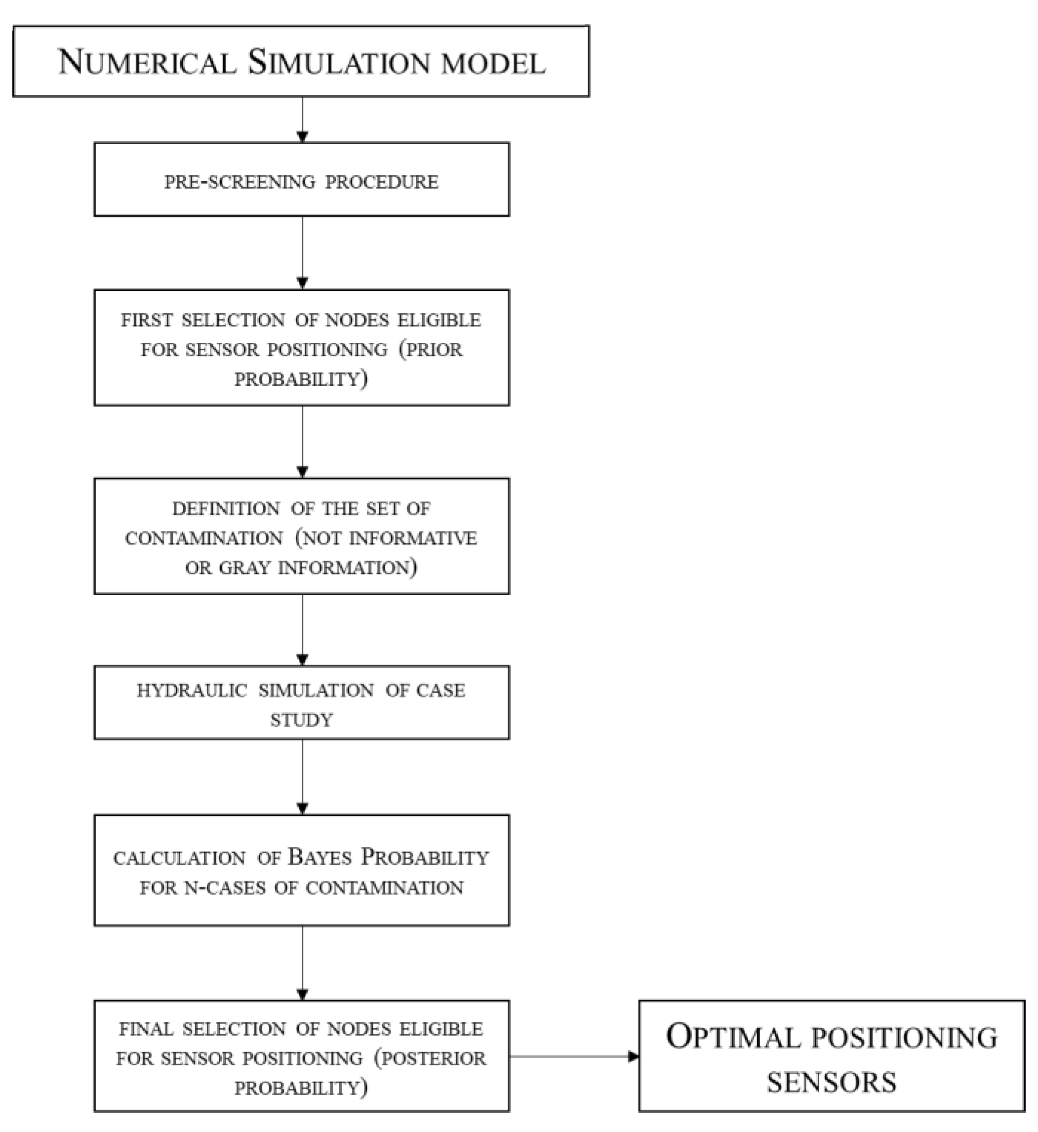
Presenting the merits of the code implemented, Figure 2 shows a flow chart that explains step by step the logic of Bayesian solver.
The first step consists in a network pre-screening procedure that allows to immediately eliminate all those nodes that are certainly not useful/strategic for the positioning of the contamination detection sensors.
In this case these nodes are:
- Outfall nodes, because clearly positioning a sensor in the terminal nodes does not give me any advantage for the purposes of rapid interception and containment of contamination;
- Head nodes, since positioning the sensors in those nodes would give a 1:1 information, i.e., it would mark a trace of contamination only if it started from that node so it would not be of help in all those other cases in which the source of contamination has started or it has moved somewhere else.
At the end of the pre-screening procedure, we obtain a first set of nodes that can be used for positioning the sensors, which however is still very large; at this point we then move on to the second step and apply the Bayesian method.
The second step consists in a further screening of nodes eligible for positioning but through the calculation of the Bayesian probability.
The origin of Bayesian philosophy lies in an interpretation of Bayes’ Theorem and it derives from two theorems, the composed probability theorem and the total probability theorem [35]:
Composed probability theorem P [A|B] = P [A ∩ B]/P [B] with P [B] > 0
Total/absolute probability theorem P [A ∩ B] = P [A|B] × P [B]
In which:
- P[A|B] is the conditional probability of A, known B. It is also called posterior probability, because it depends on the specific value of B;
- P[B|A] is the conditional probability of B, known A;
- P[A] is the prior probability or marginal probability of A. “A priori” means that it does not consider any information about B;
- P[B] is the prior probability B and acts as a normalizing constant.
Bayesian interpretation asserts that the probability of a hypothesis A conditioned upon some evidence B is equal to its likelihood P[B|A] times its probability prior to any evidence P[A], normalized by P[B]. The further claim that this is a right and proper way of adjusting our beliefs in our hypotheses given new evidence is called conditionalization. After applying Bayes’ theorem to obtain P[A|B] adopt that as your posterior degree of belief in A or, Bel[A] = P[A|B]. Conditionalization, in other words, advocates belief updating via probabilities conditional upon the available evidence. It identifies posterior probability (the probability function after incorporating the evidence, which we are writing Bel[A]) with conditional probability (the prior probability function conditional upon the evidence, which is P[A|B]).
In the present application, all network nodes were considered to have the same probability to host the contamination event, while different probabilities were established in this analysis based on the information about the system and the served area. Obviously, any different hypothesis on contamination do not impact the generality of the approach.
As in Sambito [32], each sensor network configuration was investigated by 1000 random contamination events, and its efficiency was evaluated by some indicators. The isolation likelihood F1, contamination detection F2 and sensor network reliability or redundancy F3 are expressed by the following equations:
where S is the total number of analyzed contamination events; dr is 1 if the contamination source was correctly identified by the sensor network and is 0 otherwise; dt is 1 if the contamination was correctly detected by the sensor network and is 0 otherwise; and Rr is 1 if the contamination was detected by at least two sensors and is equal to 0 otherwise. The indicator F1 provides information on the ability of the sensors network to locate the contamination source, the indicator F2 provides information on the ability of the sensor network to detect the contamination event while F3 indicates the reliability of the sensor network (more than one sensor) in detecting an event. If the contamination is not confirmed by more than one sensor in the system, false positives may be present.
As initial hypothesis on possible sensor location has a relevant impact on computational efforts, in this study, the tests are performed considering the following approaches (Prior A, B, C) to compare the results:
- Prior A: no pre-screening procedure and no prior knowledge (each node has an equal initial probability to be the location of a sensor).
- Prior B: no prior knowledge and pre-screening procedure based on network topology.
- Prior C: pre-screening procedure and prior knowledge based on water fluxes.
The Bayesian approach allows to make a further selection based substantially on the experience that the sensor has of intercepting contamination if positioned in that node, it is thus possible to identify a more restricted set of nodes based on the probability of contamination detection (posterior probability). Once a threshold has been established, only the nodes that have a greater or equal value are chosen and all those that have a lower contamination detection capacity are excluded.
If the set is still large or too small, it is possible to set a higher or lower selection threshold thus making the model flexible to the various network sizes.
2.4. Case Study
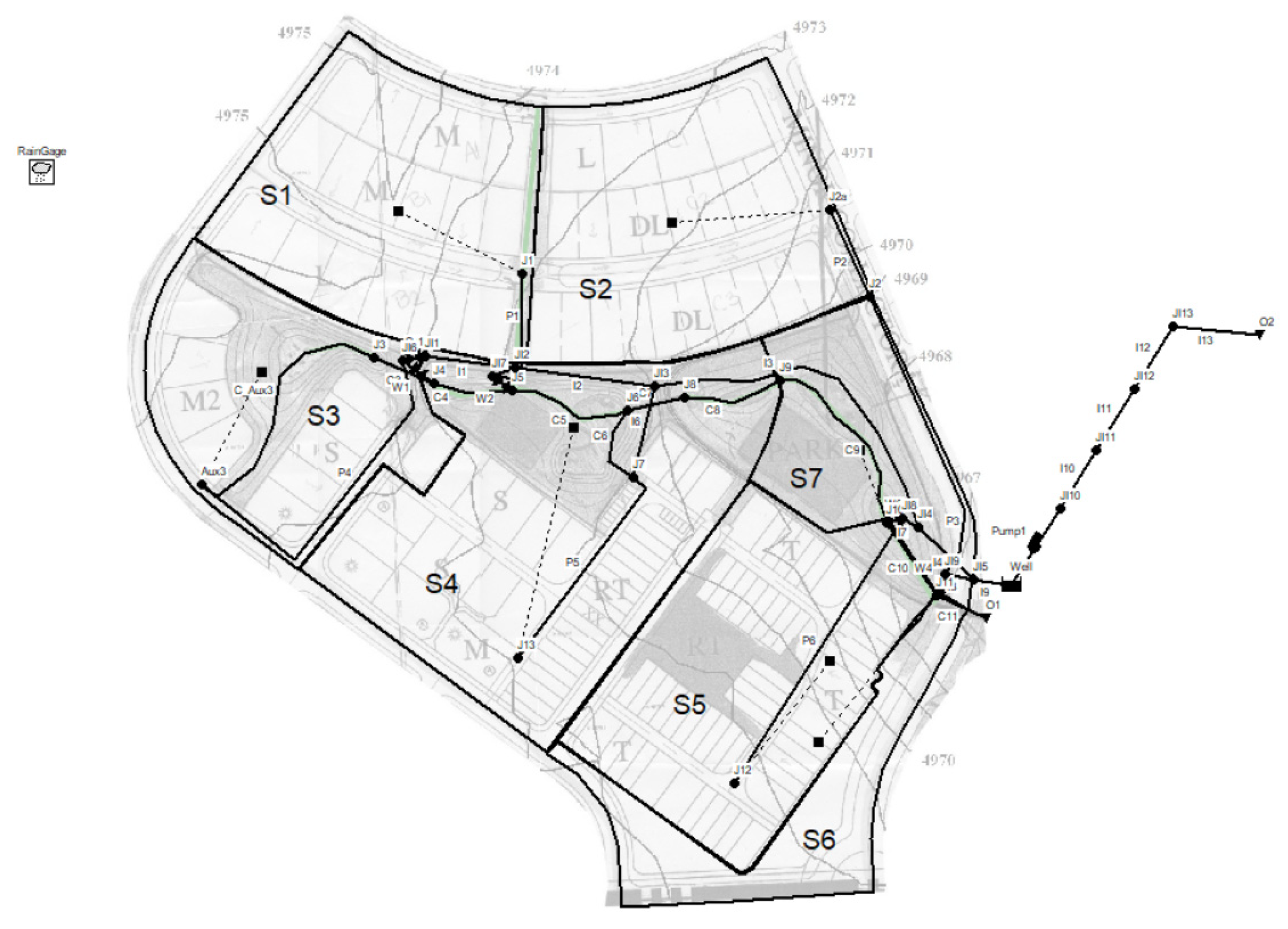
The literature Example 8, presented in the EPA SWMM reference manual, is a combined sewer system that convey both sanitary sewerage and stormwater through the same pipes. Combined sewer systems are designed to discharge the excess wastewater directly to a water body through diversion regulators. In the model, the flow regulator structures are not defined as elements directly, but through a combination of orifices, weirs and pipes. The combined sewer pipes with pipe’s name “Px” (where x represents a sequential number) are designed to capture of the sanitary and stormwater flows; the pipelines called “Interceptors” with pipe’s name “Ix”, to capture 100% of the sanitary flows during dry weather periods and convey them to a wastewater treatment plant (WWTP, O2) instead those called “stream”, where the pipes takes name “Cx”, have the task of remove the excess flows in case of combined sewer overflow and discharge them directly into the river (O1). Jx and JIx represent junctions only Aux3 has a different name as dry weather and wet weather flows are split.
The network scheme reported in Figure 3, serves an area of 0.12 km2 and consists of 31 nodes (28 junctions, 1 well and 2 outfalls), 29 pipes and a pump. The pump station is at the downstream end of the interceptor and the node “Well” is represented by a storage node and serve as the wet well for the pump station.
However, before applying the Bayesian procedure, the contamination in the network must be simulated. To this end, it is first necessary to select the node (s) that will be a source of contamination and start the hydraulic simulation in the network and as anticipated, two scenarios have been assumed. Considering that the position, magnitude and duration of contamination can be uncertain, each model application is given by a random simulation in which the contamination parameters are randomly set up in terms of the contaminant mass, contamination duration and contamination node.
In scenario 1, the xenobiotic conservative contaminant mass is randomly set between 0.1 kg and 0.5 kg; the contamination duration is randomly set between 0.25 h and 3 h.
In scenario 2, the organic non-conservative contaminant mass is randomly set between 1 kg and 3 kg; the contamination duration is randomly set between 0.25 h and 3 h. As the contaminant is supposed to be immanently present in wastewater, a constant load of 0.2 kg/h is considered from all nodes. Contaminant decay, according to Example 8 reference, is based on a first order decay law with a decay constant equal to 0.05 day−1.
3. Results and Discussion
As described in the previous paragraphs, the first step is that of the pre-screening, which is configured in the identification and elimination from the set of candidate nodes for the positioning of the contamination detection sensors, the outfalls nodes and the head nodes that are considered unlikely to be able to discriminate the location of contamination as the first group has all the network upstream and the second group has no nodes upstream.
For the case study, the nodes eliminated thanks to the initial pre-screening are 7 out of 30, that are:
- O1 and O2 which are the outfalls nodes;
- J1, J2a, Aux3, J12 and J13 which are the head nodes;
The set of nodes suitable for positioning the sensors downstream of the prescreening is therefore formed by 23 nodes. As discussed above, all the nodes (apart outfalls) have the same probability of being contaminated.
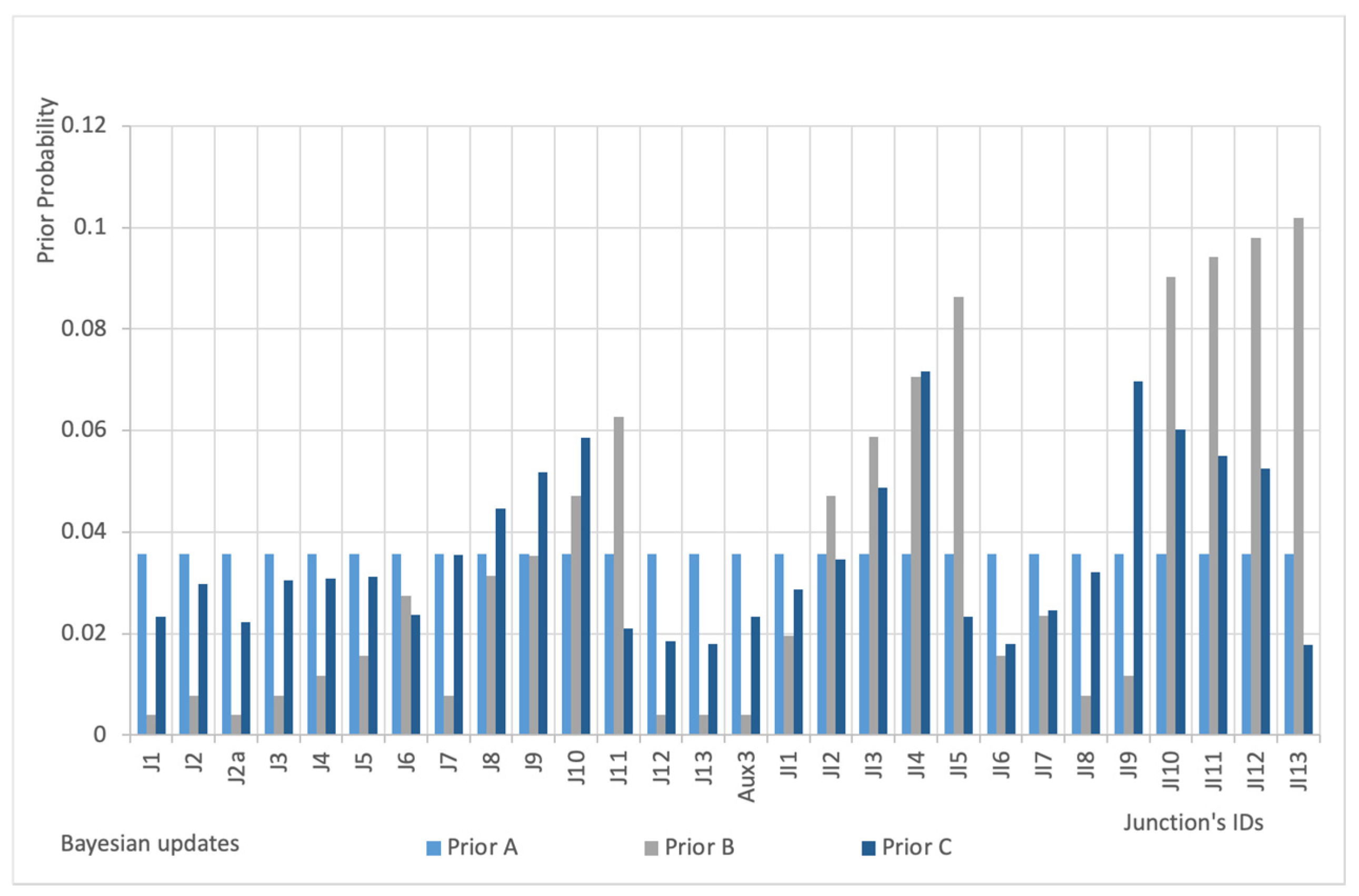
The initial step of the analysis is the definition of sensor “prior probability” according to the 3 prior hypotheses. Probability density functions are shown in Figure 4 and they are independent from the nature of contaminant. In Prior A, all the nodes have the same probability of being sensor location while Prior B and Prior C rely on some prior information based on network topology and hydraulic variables.
To evaluate the differences in terms of optimal sensor placement in the two contamination scenarios (xenobiotic conservative and immanent non-conservative), six Bayesian procedure (2 scenarios for each of the 3 prior distributions) were run in parallel considering 3 sensors to be located and running 10 update steps of 100 simulations each. After each step, the two nodes (rounded 10% of the total) with the lower posterior probabilities are removed from the analysis.
The results of Scenario 1 are quite in line with previous literature. The best locations for sensors are all in the downstream part of the network (JI10 and JI11) and the optimal sensor configuration is made up these two sensors plus a third one (JI5) in the middle part of the network (Figure 5). The results of Prior B are omitted because quite similar to Prior C.
Independently from prior distribution, the final configuration of the sensor network remains the same and it can detect 91% of contamination episodes. F1 is equal to 84% so only two contamination events for every tenth are not located. F2 is equal to 92.3% showing than when the contamination is detected, it is most likely correctly located. F3 is equal to 100% meaning that all the events were detected by at least 2 sensors and this is relevant for the reliability of the monitoring system. Differences between prior distributions are only related to the computational efforts to reach the optimal configuration: starting from the non-informative Prior A, only after 9 Bayesian updates (900 simulations), the method provides negligible updates to the posterior sensor probability distributions. Using the Prior B and C, without significant differences among them, after 5 Bayesian updates, the method only provides negligible updates and further simulations are not useful to discriminate the best location for sensors.
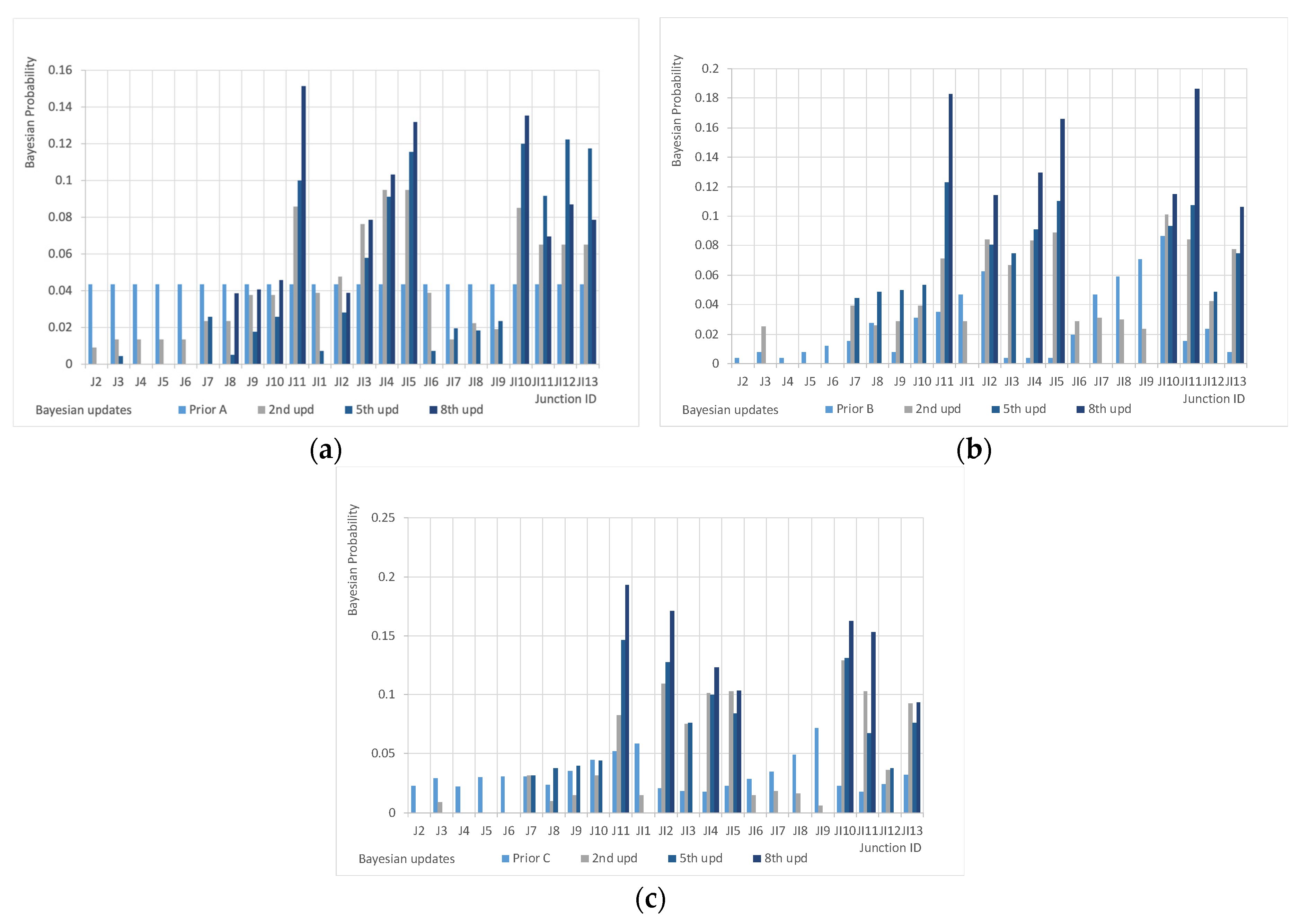
Scenario 2 provides different results: efficiencies are lower and the prior probability distribution affects slightly the optimal sensor configuration that is, in any case, different with respect to the Scenario 1.
Starting from non-informative Prior A, the best configuration is given by sensors in nodes J11, JI5 and JI10 that are no more concentrated in the downstream part of the network but distributed homogenously in the system (Figure 6). The system was able to detect only the 82% of the events because others were presumably masked by the immanent discharges in all the nodes of the system. Indicator F1 was equal to 67%—so the monitoring system was able to locate 2 events every three; the indicator F2 is equal to 81.7%—demonstrating that a large percentage of the detected events are also correctly located. Redundancy F3 drops greatly with respect to the Scenario 1 reaching only 78%.
Prior B provides a different optimal configuration in which two sensors are located in the same nodes than Prior A (J11 and JI5) and the third one is in node JI11. This last node is near to JI10 and on the same main sewer so the differences cannot be considered relevant but enough to provide better detection (85%), higher values of indicators F1 (70%) and F2 (82.3%) keeping F3 (77.8%) substantially at the same level of the previous case.
Prior C provides another optimal configuration in which two sensors are located in the same nodes than Prior A (J11 and JI10) and the third one is in node JI2. Only one node is common between Prior B and Prior C (J11). Detection capacity drops to 78%, lower values of indicators F1 (61%) and F2 (78.2%) keeping F3 (76.8%) substantially at the same level of the previous case. In none of the cases, after 10 updates, the variation of posterior probability can be considered negligible demonstrating that some other steps may be needed to help the method to improve the selection of sensor locations.
To sum up the results, Scenario 2 shows that the contamination kinetics and the presence of a continuous contribution from all nodes provide a relevant impact on sensor locations and some general comments can be provided on contamination monitoring and source locations:
- Sensor deployment is dependent on contaminant kinetics and detectability with respect to background concentration so that more dense and uniformly distributed networks are expected when degradable and immanent contaminants need to be investigated;
- Xenobiotic conservative contaminations are easier to be located provided that sensor technology is sufficiently reliable and that networks can be deployed in downstream nodes so a smaller number of sensors is able to investigate large portions of the drainage system;
- The Bayesian approach gives its best in this type of problem, in which the initial database is small and only general and non-formal information is available about polluting sources; the method is able to introduce information coming from the initial detection exercises to improve the network in time thus allowing for deploying an initial sensor network configuration to be updated once a sufficient number of events are detected.
4. Conclusions
The goal of this study was to investigate Bayesian methods to identify optimal sensor distribution to solve a contamination detection and location problem. Some examples in literature relies on the simplified hypothesis of considering xenobiotic soluble conservative contaminants that are not usually present in the sewers system (such as metals). In this study, a non-conservative and immanent contaminant was considered (such as organic carbon or nitrogen) that is usually present in urban wastewater but that may be the object of illicit contamination when loads are higher than what is authorized by law.
In such a case, two problems have to be faced by the monitoring system: the decay of the contaminant, so that the path is longer from the contamination node and the sensor and the chances are smaller to detect it; and the presence of distributed loads of the same contaminant that is illicitly discharged so downstream sensors are less efficient in the location exercise.
The method demonstrated to be versatile being able to obtain significant results both in the conservative and in the non-conservative scenario. Some interesting considerations may arise from the comparison of the two cases:
- The selection of prior distribution is irrelevant for the selection of the optimal sensor configuration in the conservative scenario while affects results in the non-conservative case; differences are not great (with the Prior B outperforming the others) but they are not negligible.
- Prior C based on flows probably does not adequately address the fact that with bigger flows, the sensor may be unable to detect the contamination due to the masking effect of distributed discharges of the same chemical.
- The number of steps needed to achieve the optimal configuration is much higher in the non-conservative case, showing the presence of greater uncertainties, and results are worse even if still largely acceptable.
- The two sensor configurations are different with the conservative case privileging the downstream nodes and the non-conservative one suggesting a more balanced configuration. This demonstrates that the nature of contaminant is a relevant information for deploying the best possible sensing strategy.
The study showed that some nodes can be considered a good starting point for any monitoring network as they demonstrated to be relevant both in case of conservative and non-conservative contaminants. Some others have to be selected depending on the contaminant that has to be searched.
In conclusion, the methodology should be upgraded and tested to take into account the presence of multiple contamination sources and the possibility of deploying Lagrangian sensors carried by the flow. Additionally, the comparison with fault isolation approaches [36] may be interesting from the perspective of transferring the fault mode and effect analysis (FMEA)-type approaches to the water industry.
Author Contributions
M.S., G.F. equally contributed to the present research and to the preparation of the paper. All authors have read and agreed to the published version of the manuscript.
Funding
This research received no external funding.
Data Availability Statement
Data sharing not applicable.
Conflicts of Interest
The authors declare no conflict of interest.
References
- Passerat, J.; Ouattara, N.K.; Mouchel, J.-M.; Rocher, V. Impact of an intense combined sewer overflow event on the microbiological water quality of the Seine River. Water Res. 2011, 45, 893–903. [Google Scholar] [CrossRef] [PubMed]
- Piazza, S.; Mirjam Blokker, E.J.; Freni, G.; Puleo, V.; Sambito, M. Impact of diffusion and dispersion of contaminants in water distribution networks modelling and monitoring. Water Sci. Technol. Water Supply 2020, 20, 46–58. [Google Scholar] [CrossRef]
- Francés-Chust, J.; Carpitellan, S.; Herrera, M.; Izquierdo, J.; Montalvo, I. Optimal placement of quality sensors in water distribution systems. In Proceedings of the Conference: Mathematical Modelling Conference in Engineering & Human Behaviour, Valencia, Spain, 10–12 July 2019. [Google Scholar]
- Lifshitz, R.; Ostfeld, A. Clustering for real time response to water distribution system contamination event intrusion. J. Water Resour. Plan. Manag. 2019, 145, 04018091. [Google Scholar] [CrossRef]
- Piazza, S.; Sambito, M.; Feo, R.; Freni, G.; Puleo, V. Optimal positioning of water quality sensors in water distribution networks: Comparison of numerical and experimental results. In Proceedings of the CCWI 2017—15th International Conference on Computing and Control for the Water Industry, Sheffield, UK, 5–7 September 2017. [Google Scholar]
- Bourgeois, W.; Burgess, J.E.; Stuetz, R.M. On-line monitoring of wastewater quality: A review. J. Chem. Technol. Biotechnol. 2001, 76, 337–348. [Google Scholar] [CrossRef]
- Shahriari, B.; Swersky, K.; Wang, Z.; Adams, R.P.; de Freitas, N. Taking the human out of the loop: A review of Bayesian optimization. Proc. IEEE 2016, 104, 148–175. [Google Scholar] [CrossRef] [Green Version]
- Brochu, E.; Brochu, T.; de Freitas, N. A Bayesian interactive optimization approach to procedural animation design. In Proceedings of the 2010 ACM SIGGRAPH/Eurographics Symposium on Computer Animation, Madrid, Spain, 2–4 July 2010; pp. 103–112. [Google Scholar]
- Lizotte, D.; Wang, T.; Bowling, M.; Schuurmans, D. Automatic gait optimization with Gaussian process regression. In Proceedings of the 20th International Joint Conference on Artificial Intelligence, Hyderabad, India, 6–12 January 2007; pp. 944–949. [Google Scholar]
- Martinez-Cantin, R.; de Freitas, N.; Doucet, A.; Castellanos, J.A. Active policy learning for robot planning and exploration under uncertainty. Proc. Robot. Sci. Syst. 2007, 3, 321–328. [Google Scholar]
- Marchant, R.; Ramos, F. Bayesian optimization for intelligent environmental monitoring. In Proceedings of the IEEE/RSJ International Conference on Intelligent Robots and Systems, Vilamoura-Algarve, Portugal, 7–12 October 2012; pp. 2242–2249. [Google Scholar] [CrossRef]
- Wang, Z.; Shakibi, B.; Jin, L.; de Freitas, N. Bayesian multi-scale optimistic optimization. In Proceedings of the 17th International Conference on Artificial Intelligence and Statistics (AISTATS), Reykjavic, Iceland, 22–25 April 2014; pp. 1005–1014. [Google Scholar]
- Hutter, F.; Hoos, H.H.; Leyton-Brown, K. Sequential Model-based Optimization for General Algorithm Configuration, Learning and Intelligent Optimization; Springer: Berlin, Germany, 2011; pp. 507–523. [Google Scholar]
- Wang, Z.; Zoghi, M.; Matheson, D.; Hutter, F.; de Freitas, N. Bayesian optimization in high dimensions via random embeddings. In Proceedings of the Twenty-Third International Joint Conference on Artificial Intelligence, Beijing, China, 3–9 August 2013; pp. 1778–1784. [Google Scholar]
- Bergstra, J.; Bardenet, R.; Bengio, Y.; Kegl, B. Algorithms for hyper-parameter optimization. In Proceedings of the 25th Annual Conference on Neural Information Processing Systems (NIPS 2011), Granada, Spain, 12–17 December 2011; pp. 2546–2554. [Google Scholar]
- Hoffman, M.; Shahriari, B.; de Freitas, N. On correlation and budget constraints in model-based bandit optimization with application to automatic machine learning. In Proceedings of the 17th International Conference on Artificial Intelligence and Statistics (AISTATS), Reykjavic, Iceland, 22–25 April 2014; pp. 365–374. [Google Scholar]
- Snoek, J.; Larochelle, H.; Adams, R.P. Practical Bayesian optimization of machine learning algorithms. In Proceedings of the 25th International Conference on Neural Information Processing Systems, New York, NY, USA, 3–6 December 2012; Volume 2, pp. 2951–2959. [Google Scholar]
- Swersky, K.; Snoek, J.; Adams, R.P. Multi-task Bayesian optimization. In Proceedings of the Neural Information Processing Systems, Harrahs and Harveys, Lake Tahoe, CA, USA, 5–10 December 2013; pp. 2004–2012. [Google Scholar]
- Thornton, C.; Hutter, F.; Hoos, H.H.; Leyton-Brown, K. Auto-WEKA: Combined selection and hyperparameter optimization of classification algorithms. In Proceedings of the 19th ACM SIGKDD International Conference on Knowledge Discovery and Data Mining, Chicago, IL, USA, 11 August 2013; pp. 847–855. [Google Scholar]
- Garnett, R.; Osborne, M.A.; Roberts, S.J. Bayesian optimization for sensor set selection. In Proceedings of the 9th ACM/IEEE International Conference on Information Processing in Sensor Networks; Association for Computing Machinery: New York, NY, USA, 2010; pp. 209–219. [Google Scholar]
- Srinivas, N.; Krause, A.; Kakade, S.M.; Seeger, M. Gaussian process optimization in the bandit setting: No regret and experimental design. In Proceedings of the 27th International Conference on Machine Learning, Haifa, Israel, 21–24 June 2010; pp. 1015–1022. [Google Scholar]
- Mahendran, N.; Wang, Z.; Hamze, F.; de Freitas, N. Adaptive MCMC with Bayesian optimization. J. Mach. Learn. Res. 2012, 22, 751–760. [Google Scholar]
- Azimi, J.; Jalali, A.; Fern, X. Hybrid batch Bayesian optimization. In Proceedings of the 29th International Conference on Machine Learning, Edinburgh, UK, 26 June–1 July 2012; pp. 1215–1222. [Google Scholar]
- Brochu, E.; Cora, V.M.; de Freitas, N. A Tutorial on Bayesian Optimization of Expensive Cost Functions, with Application to Active User Modeling and Hierarchical Reinforcement Learning; Technical Report UBC TR-2009-23; Department of Computer Science, University of British Columbia: Vancouver, BC, Canada, 2009. [Google Scholar]
- Marsalek, J.; Rochfort, Q. Urban wet-weather flows: Sources of fecal contamination impacting on recreational waters and threatening drinking-water sources. J. Toxicol. Environ. Health A 2004, 67, 1765–1777. [Google Scholar] [CrossRef] [PubMed]
- Nawrot, N.; Wojciechowska, E.; Rezania, S.; Walkusz-Miotk, J.; Pazdro, K. The effects of urban vehicle traffic on heavy metal contamination in road sweeping waste and bottom sediments of retention tanks. Sci. Total Environ. 2020, 749, 141511. [Google Scholar] [CrossRef] [PubMed]
- Cryder, Z.; Greenberg, L.; Richards, J.; Wolf, D.; Luo, Y.; Gan, J. Fiproles in urban surface runoff: Understanding sources and causes of contamination. Environ. Pollut. 2019, 250, 754–761. [Google Scholar] [CrossRef] [PubMed]
- Ghane, E.; Ranaivoson, A.Z.; Feyereisen, G.W.; Rosen, C.J.; Moncrief, J.F. Comparison of Contaminant Transport in Agricultural Drainage Water and Urban Stormwater Runoff. PLoS ONE 2016, 11. [Google Scholar] [CrossRef] [PubMed]
- Su, X.; Sutarlie, L.; Loh, X.J. Sensors, Biosensors, and Analytical Technologies for Aquaculture Water Quality. Research 2020, 8272705. [Google Scholar] [CrossRef] [PubMed] [Green Version]
- Pasika, S.; Gandla, S.T. Smart water quality monitoring system with cost-effective using IoT. Heliyon 2020, 6, e04096. [Google Scholar] [CrossRef] [PubMed]
- Yu, H.C.; Tsai, M.Y.; Tsai, Y.C.; You, J.J.; Cheng, C.L.; Wang, J.H.; Li, S.J. Development of Miniaturized Water Quality Monitoring System Using Wireless Communication. Sensors 2019, 19, 3758. [Google Scholar] [CrossRef] [PubMed] [Green Version]
- Sambito, M.; Di Cristo, C.; Freni, G.; Leopardi, A. Optimal water quality sensor positioning in urban drainage systems. J. Hydroinform. 2020, 22, 46–60. [Google Scholar] [CrossRef]
- Gironás, J.; Roesner, L.A.; Davis, J.; Rossman, L.A.; Supply, W. Storm Water Management Model Applications Manual; National Risk Management Research Laboratory, Office of Research and Development, US Environmental Protection Agency: Cincinnati, OH, USA, 2009.
- Riano-Briceno, G.; Barreiro-Gomeza, J.; Ramirez-Jaimea, A.; Quijanoa, N.; Ocampo-Martinez, C. MatSWMM—An Open-Source Toolbox for Designing Real-Time Control of Urban Drainage Systems. Environ. Model. Softw. 2016, 83, 143–154. [Google Scholar] [CrossRef] [Green Version]
- Korb, K.B.; Nicholson, A.E. Bayesian Artificial Intelligence, 2nd ed.; CRC Press: Boca Raton, FL, USA, 2010. [Google Scholar]
- Blanke, M.; Kinnaert, M.; Lunze, J.; Staroswiecki, M. Diagnosis and Fault-Tolerant Control, 3rd ed.; Springer: Berlin/Heidelberg, Germany, 2015. [Google Scholar] [CrossRef] [Green Version]
Figure 1.
Corresponding folders and files of the MatSWMM toolbox. SWMM, Storm Water Management Model
Figure 1.
Corresponding folders and files of the MatSWMM toolbox. SWMM, Storm Water Management Model

Figure 2.
Flow chart of numerical simulation model.

Figure 3.
Example 8 network scheme.

Figure 4.
Prior probability density function.

Figure 5.
Posterior probabilities in Scenario 1.A (a) and 1.C (b).

Figure 6.
Posterior probabilities in Scenario 2.A (a), 2.B (b). and 2.C (c).


Table 1.
Main differences between pressurized distribution networks and free surface networks.
| Pressurized Distribution Networks | Free Surface Networks | |
|---|---|---|
| Contamination episodes | Water leak from loss of pressure or household pipes/hospitals/etc. and voluntary contamination. | Illicit discharges from private or industrial and commercial activities, in sewer systems. |
| Contaminants | Microbial pathogens from fecal contamination, aquatic microorganisms and their toxins, chemical contaminants. | Untreated domestic and industrial waste, toxic materials and debris. |
| Modelling | The solutions space is known a priori, it may be a backward contamination and the flow has low variations. | The solutions space is not known a priori, it cannot be a backward contamination and the flow has high variations. |
| Impact of contamination | Resources and public health. | Sewer system, wastewater treatment plant and water body. |
| Sensor technology | Fixed type sensors. | Fixed, mobile type sensors or sampling. |
Publisher’s Note: MDPI stays neutral with regard to jurisdictional claims in published maps and institutional affiliations. |
© 2021 by the authors. Licensee MDPI, Basel, Switzerland. This article is an open access article distributed under the terms and conditions of the Creative Commons Attribution (CC BY) license (https://creativecommons.org/licenses/by/4.0/).
Share and Cite
MDPI and ACS Style
Sambito, M.; Freni, G. Strategies for Improving Optimal Positioning of Quality Sensors in Urban Drainage Systems for Non-Conservative Contaminants. Water 2021, 13, 934. https://doi.org/10.3390/w13070934
AMA Style
Sambito M, Freni G. Strategies for Improving Optimal Positioning of Quality Sensors in Urban Drainage Systems for Non-Conservative Contaminants. Water. 2021; 13(7):934. https://doi.org/10.3390/w13070934
Chicago/Turabian StyleSambito, Mariacrocetta, and Gabriele Freni. 2021. "Strategies for Improving Optimal Positioning of Quality Sensors in Urban Drainage Systems for Non-Conservative Contaminants" Water 13, no. 7: 934. https://doi.org/10.3390/w13070934
Note that from the first issue of 2016, this journal uses article numbers instead of page numbers. See further details here.