
Numerical and Experimental Investigations of Flow Pattern and Anti-Vortex Measures of Forebay in a Multi-Unit Pumping Station


1
College of Hydraulic Science and Engineering, Yangzhou University, Yangzhou 225009, China
2
Key Laboratory of Fluid and Power Machinery, Ministry of Education, Chengdu 610039, China
3
Hydrodynamic Engineering Laboratory of Jiangsu Province, Yangzhou University, Yangzhou 225009, China
4
Jiangsu Surveying and Design Institute of Water Resources Co., Ltd., Yangzhou 225127, China
*
Author to whom correspondence should be addressed.
Water 2021, 13(7), 935; https://doi.org/10.3390/w13070935
Submission received: 24 January 2021
/
Revised: 17 March 2021
/
Accepted: 26 March 2021
/
Published: 29 March 2021
(This article belongs to the Section Hydraulics and Hydrodynamics)
Abstract
:The forebay of a pumping station is an important building connecting the diversion channel and the intake pool. Based on the physical model test and research method of computational fluid dynamics (CFD) based on the improved fluid volume model, the flow field in a forebay of a multi-unit pumping station is analyzed in combination with the engineering practice of the Exi River flood discharge station in the Anhui Province, China. Aiming at the technical problems of a large-scale swing water area in the forebay internal flow field of a lateral intake pumping station, the technical problems are discussed. Different rectification measures are selected to adjust the flow pattern in the forebay of a pumping station. The internal rectification flow pattern in the forebay under different plans, the uniformity of flow velocity distribution in the measurement section, and the reduction rate of the vortex area are studied and compared, and the optimal plan is given. The results show that the flow pattern of the 7.5 m and 15 m solutions of the lengthened inflow wall is still poor, and the ability to eliminate vortices is not strong or even counterproductive. The combination plan of a rectifier sill and a rectifier pier has a better effect and can eliminate more than 90% of the vortex, but the uniformity of flow speed has not been significantly improved at the inlet of the pumping station; the combination plan of a rectifier sill and a diversion wall opening has the best effect; the reduction rate of the vortex area is more than 85%, and the velocity uniformity of three measuring sections is better than that of the original plan. The uniformity of flow rate near the pumping station is increased by 4% and that far away from the pumping station is increased by 13%. The combination plan of a rectifier sill and diversion wall with openings is recommended.
1. Introduction
As an important public welfare infrastructure for national economic and social development, a drainage pumping station is an important component of people’s livelihood and water conservancy, as well as an important component of flood control and waterlogging control system. According to the statistics of renovation and renovation of large-scale irrigation and drainage pumping stations in China, 327 large-scale drainage and irrigation-and-drainage combined pumping stations have been built, with an installed power of 29.191 million kW and a design total flow of 31,941.5 m3/s; the effective drainage area is about 9.13 million hm2, accounting for 42.9% of the total drainage area in China; the average annual drainage of large-scale drainage pumping stations is more than 40 billion m3, which protects the life and property safety of more than 200 cities and more than 150 million people in China [1,2].
The intake forebay is an important part of a pumping station. Its main function is to guide water flow smoothly into the intake basin of the pumping station and ensure good intake conditions of the pump [3]. The flow pattern of the pumping station forebay directly affects the hydraulic performance, operating efficiency, and service life of the pumping station, and even affects the normal operation of the pumping station [4,5]. However, with global warming, the frequency of extreme weather events is increasing, and flooding disasters are showing a more frequent trend, which puts more pressure on some older pumping stations, especially on the flow pattern of the forebay at high water level.
Regarding the flow pattern in the front pool of a pumping station, in the past, the analysis mainly relied on physical model tests, usually using flow velocity meters to measure the flow velocity at distribution points or applying Particle Image Velocimetry (PIV) and Laser Doppler Anemometry (LDA) to display the flow field. In recent years, computational fluid dynamics (CFD) numerical simulations have become a common research tool in order to improve analysis efficiency and study the flow field in a more detailed manner. At present, scholars and engineers in this field have carried out some research on the flow pattern and rectification measures of water flow in the front pool of pumping stations: Chen et al. [6] conducted a simulation study on the flow pattern and velocity distribution of each section inside the inlet pool of pumping stations, which showed that the flow pattern of the inlet pool could be improved by adding a guide pier and a W-shaped back wall in the rectangular inlet pool. Zhou et al. [7] applied the CFX software for a lateral inlet pumping station based on the Reynolds time-averaged N–S equation and the standard k–ε turbulence model to numerically simulate the front pool flow pattern and analyzed and determined the deflecting wall as the optimal flow rectification scheme. Luo et al. [8] used the CFD technology to numerically simulate the flow patterns of the prototype forebay and inlet pool for a combined lateral inlet pumping station and analyzed and selected the combined rectification measures of a three-section isolation pier, column, and rear bulkhead. Xia et al. [9] applied the Fluent software for a positive inlet pumping station based on the Re-normalization Group (RNG) k–ε model to numerically simulate the front pool flow pattern with the addition of a single-row square column and analyzed the effect of the geometric parameters of a single-row square column on the improvement of the front pool flow pattern; the study showed that the addition of a single-row square column in the front pool could significantly improve the flow pattern. Luo et al. [10] showed that the flow pattern could be better adjusted by the combination of columns and the bottom canal based on the model test. Constantinescu et al. [11] used the standard k–ε equation to numerically simulate the vortex in the front pool of a pumping station, and the simulated vortex structure in the pool was consistent with the results obtained from the model test. Kadam et al. [12] used physical model tests combined with numerical simulation techniques to study the flow field of the inlet building of a pumping station and observed the flow characteristics of the forebay and the inlet pipe, and found that the excessive diffusion angle of the forebay and small inundation depth made the inlet flow pattern poor.
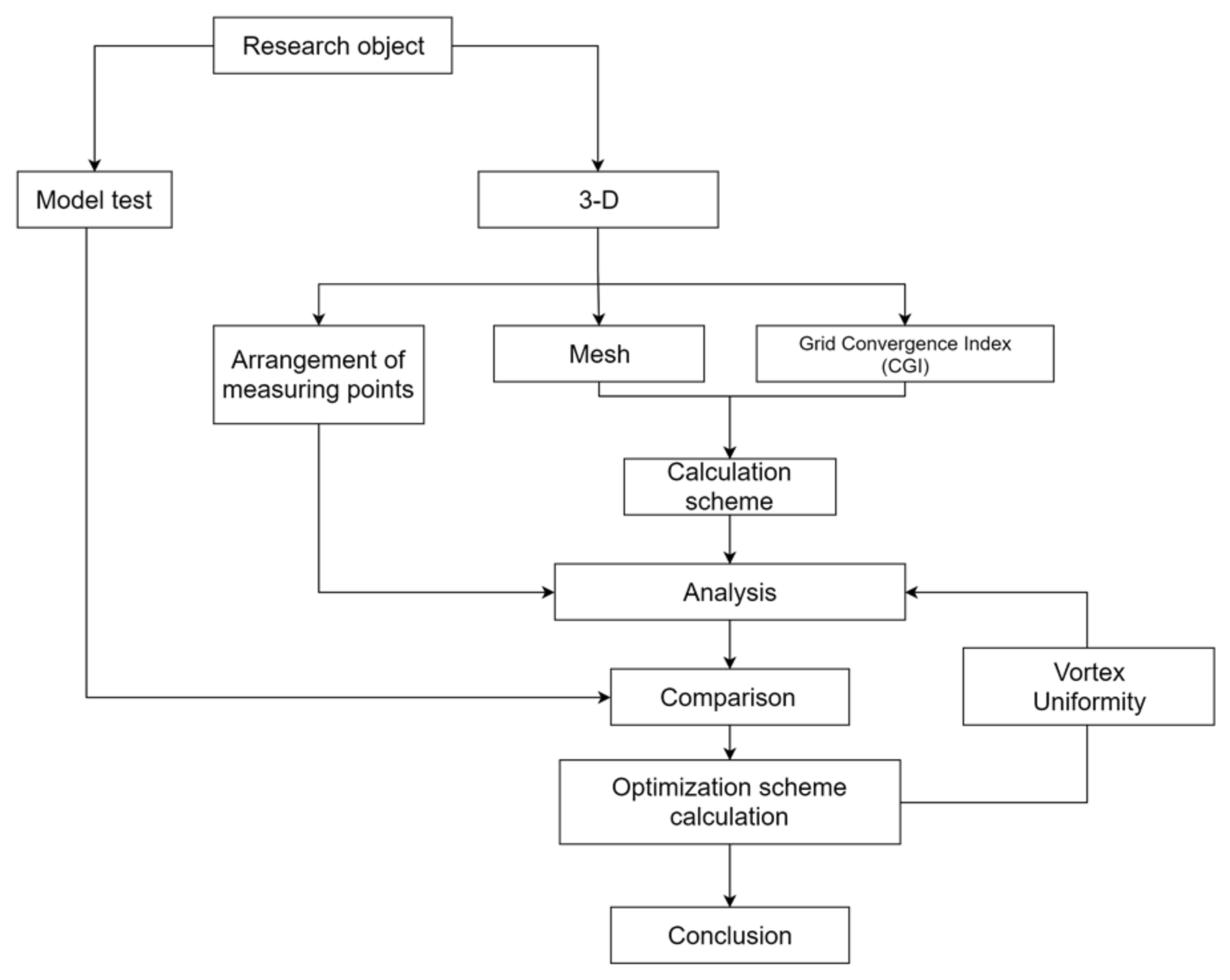
This paper takes the Exi River Flood Discharge Station in the Anhui Province as the research object, improves and optimizes the hydraulic performance of the forebay in the original design plan based on the improved volume of fluid (VOF) model combined with a three-dimensional turbulence numerical model and a physical model test, and explores the combined strategy of a diversion wall, a rectifier sill, and a rectifier pier to control the flow field in the forebay of the pumping station under various conditions by the CFD method. The analysis method and procedure are shown in Figure 1.
The innovation of this research lies in the combination of a model test and a numerical simulation, which combines the flow improvement of streamline judgment with the analysis of the vortex area and flow uniformity. This article contains four chapters, Engineering Background, Mathematical Formulation, Physical Model Test and Numerical Simulation, and Results and Discussion. It provides reference for related pumping station engineering.
2. Engineering Background
2.1. Importance of Engineering
The Exi River belongs to the second branch of the Yangtze River, with a total area of 169 km2, including land area over 10,000 mu. The river basin is located in the humid monsoon climate zone in the north subtropical zone, with temperate and humid climate, abundant rainfall, moderate light, obviously monsoon climate, and the annual average rainfall of 1275 mm. As the area of the mountainous catchment in the Exi River basin is too large and the flood storage capacity of the river is small, there have been many major disasters in the history of the river basin. For example, the main city of the Fanchang County in the river basin and most of the county cities were flooded during the flood season of 1983 and 1999, and in 2016, the danger of exceeding the warning water level of 0.46 m occurred. Therefore, it is very necessary to strengthen the flood control and flood preparedness of the relevant flood control and drainage gate stations.
The Exi River flood discharge station (Figure 2) is a constructive management project for post-disaster water conservancy weaknesses in the Anhui Province approved by the Anhui Provincial Government which expands the outflow capacity of the Exi River and improves the overall flood control standard and flood mitigation capacity of the basin. It is conducive to reducing flood losses at the basin scale, safeguarding the lives and properties of people in urban and rural areas in the basin, and ensuring flood control safety and sustainable socioeconomic development in the Anhui Province.
2.2. Project Scale and Parameters
The flood control standard of the Exi River flood discharge station is designed once in 50 years and checked once in 200 years. Four sets of shaft tubular units are installed in the pumping station. Pump impeller diameter is 3.00 m. Four sets of units are arranged on one floor with 9.2 m unit spacing, 5.4 m pump impeller center elevation, 26.05 m3/s single unit design flow, 1250 kW auxiliary motor power, and 5000 kW total installed capacity. The characteristic water level is shown in Table 1.
3. Mathematical Formulation
The three-dimensional hydrodynamic model is a complete description of the flow process of the water body. The main control equations include:
3.1. Mass Continuity Equation
For incompressible fluids:
where (u, v, w) are the instantaneous velocity components in the horizontal and vertical (x, y, z) directions, respectively; Ax is the fractional area open to flow in the X-direction and Ay and Az are similar area fractions for flow in the Y- and Z-directions; R is set to unity; ξ is set to zero; RSOR is the mass source.
3.2. Momentum Equations
The equations of motion for the fluid velocity components (u, v, w) in the three coordinate directions are the Navier–Stokes equations with some additional items:
In these equations:
(Gx, Gy, Gz) are body accelerations; (fx, fy, fz) are viscous accelerations; VF is the fractional volume open to flow; ρ is the fluid density.
Uw = (uw, vw, ww) is the velocity of the source component.
Us = (us, vs, ws) is the velocity of the fluid at the surface of the source relative to the source itself. It is computed in each control volume as
where dQ is the mass flow rate; ρQ is the fluid source density; dA is the area of the source surface in the cell; and n is the outward normal to the surface. When d = 0.0 in Equation (3), the source is of the stagnation pressure type. If d = 1.0, the source is of the static pressure type.
3.3. Turbulence Transport Models
The one-equation turbulence transport model consists of a transport equation for the specific kinetic energy associated with turbulent velocity fluctuations in the flow (the turbulent kinetic energy):
where u′, v′, w′ are the x, y, z components of the fluid velocity associated with chaotic turbulent fluctuations.
The transport equation for kT includes the convection and diffusion of the turbulent kinetic energy, the production of turbulent kinetic energy due to shearing and buoyancy effects, diffusion, and dissipation due to viscous losses within turbulent eddies. Buoyancy production only occurs if there is a non-uniform density in the flow and includes the effects of gravity and non-inertial accelerations. The transport equation is:
GT is the buoyancy production:
where μ is the molecular dynamic viscosity; ρ is the fluid density; P is the pressure; and CRHO is another turbulence parameter, whose default value is 0.0, so for incompressible liquids, is zero.
The diffusion term is expressed as
where is the diffusion coefficient of and is computed based on the local value of the turbulent viscosity. Its value defaults to 1.0.
PT is the turbulent kinetic energy production:
where CSPRO is a turbulence parameter, whose default value is 1.0; R and ξ were described earlier in the Mass Continuity Equation section and are related to the cylindrical coordinate system; Ax is the fractional area open to flow in the X-direction, Ay and Az are similar area fractions for flow in the Y- and Z-directions.
Because turbulence enhances the diffusion of momentum, it effectively enhances the viscosity. Wherever the coefficient of dynamic viscosity appears in the equations, we assume that it is a sum of the molecular and turbulent viscosities:
3.4. VOF Fluid Interfaces and Free Surfaces
Fluid configurations are defined in terms of a volume of fluid (VOF) function, F (x, y, z, t). This function represents the volume of fluid per unit volume and satisfies the equation
where
The diffusion coefficient is defined as νF = cF μ/ρ, where cF is a constant whose reciprocal is sometimes referred to as a turbulent Schmidt number. This diffusion term only makes sense for the turbulent mixing of two fluids whose distribution is defined by the F function, the fluid exists when F = 1, and void regions correspond to locations where F = 0.
FSOR corresponds to the density source RSOR in Equation (1); FSOR is the time rate of change of the volume fraction of fluid associated with the mass source for fluid.
4. Physical Model Test and Numerical Simulation
4.1. Model Test
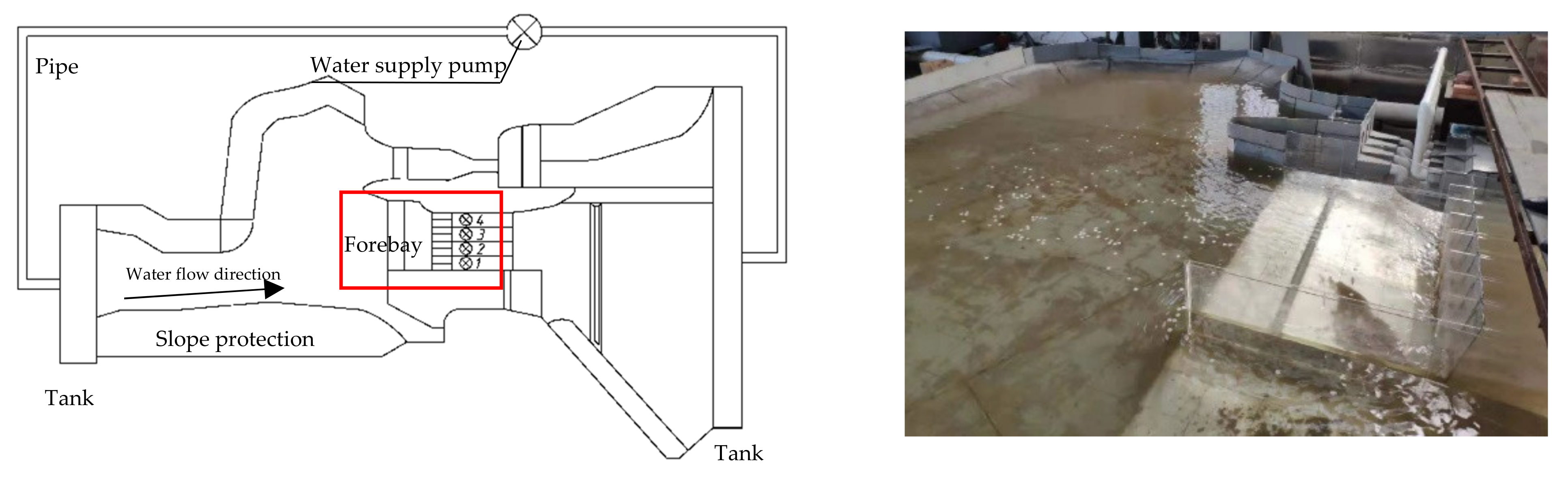
The scope of the hydraulic model test includes new flood discharge station for the Exi River and the affected area. The engineering area of the gate station includes upstream and downstream diversion of the river (total length about 300 m), and the vertical flow direction of the project area includes embankments on both sides of the diverted river (total width about 200 m). The main structures include the existing flood discharge West station, the railway bridge, the proposed new flood discharge station, and the control gate. The actual simulation range of the model is about 500 m long, including the upstream and downstream diversion sections, the inlet diversion section, the forebay, the pump chamber, the sluice control, the diversion wall, the stilling basin, and the scour prevention trough, and about 300 m wide, including embankments on both sides of the diversion channel. As shown in Figure 3, the model test system will be #1, #2, #3, and #4 in turn towards the pumping station inlet away from the diversion wall.
4.1.1. Similarity Criteria and Scales
To ensure that the flow of the model is similar to that of the prototype, the boundary conditions and stress conditions of both must be similar, i.e., certain similar conditions and similar criteria must be observed in the model test. Generally, to make the model and the prototype flow exactly the same, three basic conditions must be met, namely, geometric similarity, kinematic similarity, and dynamic similarity, as well as the Reynolds similarity principle, the Froude similarity rule, the Eu similarity rule, and the Strouhal similarity rule. For this model test, as the main force on the water flow is gravity, the gravity similarity criterion is used, and to ensure that various local hydraulic phenomena of the water flow remain similar, the normal model was used, and the model was designed according to the Froude similarity rule: .
According to the dimension and plane layout of the new Exi River flood discharge station, the geometric scale of the model is determined using the law of gravity similarity. The total length and width of the model were about 7 m and 4 m respectively. According to the similarity criteria:
Geometric scale:
Velocity scale:
Time scale:
Quantity scale:
Roughness scale:
The prototype used reinforced concrete with roughness , then the corresponding roughness coefficient range of the model should have been:
According to the above data, the model was made with high-quality acrylic force and PVC grey board (its roughness coefficient , which can meet the test requirements.
4.1.2. Velocity Measuring System
This experiment adopts large-scale particle image velocimetry (LSPIV), which is an image-based surface imaging velocimetry technology with the characteristics of instantaneous full-field flow velocity measurement, and has obvious advantages in rapidly acquiring instantaneous flow field, turbulence characteristics, and flow patterns. The LSPIV can acquire the flow distribution on the surface of the lateral inlet forebay in real time and obtain a large range of quantitative flow velocity distribution. Compared with the flow velocity meter and Acoustic Doppler Velocimetry (ADV) single-point velocity measurement equipment, the LSPIV measurement system can acquire the whole field data at one time, and it is a non-contact measurement, avoiding the interference of the test equipment with the flow field. Maximum field of view of the system: 5 m × 5 m. The surface flow of the intake forebay is chaotic and accompanied by many eddies, which makes it impossible to measure all instantaneous flow fields by conventional techniques. The system combines image recognition technology, particle image velocity measurement technology, and particle tracking speed measurement technology to achieve image tracking-related processing and refine flow field velocity distribution. At present, the large-scale particle image velocity measurement system has been applied by many scholars to measure the velocity distribution on the river surface and achieved good results.
The camera uses a U.S. Phantom VEO 710 digital camera with a resolution of 1280 × 800 pixels and a full frame shooting rate of 7400 frames/second, which ensures the image details required for the identification and tracking of water surface tracers at large scales and can complete the acquisition of image sequences, acquisition of flow velocity fields, and estimation of flow rates within seconds. A preset master clock divider is used to generate a pulse signal to trigger the shutter of the image sensor in hardware to achieve a single frame exposure, ensuring accurate interframe timing and precise flow rate measurement. The tracer particles are dispersed on the surface layer, and then the trajectory is collected by LSPIV and analyzed by software to obtain the flow field vector map of the corresponding area. However, in the physical model test, the angle of the camera is fixed, and when the particles are tracked to the edge, they are not photographed, causing part of the stream to end at the edge wall. The restriction distance is about 0.05–0.1 m. This is a limitation of the experimental method close to the walls, see the figure in Chapter 4 for details.
The system adopts an advanced digital image processing algorithm and a particle tracking algorithm combined with the basic theory of fluid mechanics to collect multi-channel flow field data at the same time, which has high measurement efficiency and accuracy, and the system is suitable for the measurement of surface flow field of large physical model test.
4.2. Numerical Simulation
4.2.1. 3D Modeling
The first step in numerical simulation is the modeling of three-dimensional entities. It is an important factor affecting the lattice division and the accuracy of the final research results whether the model is accurate or not [13,14]. After the model is established, the three-dimensional boundary conditions are compared with references [15] as the flow velocity and pressure of the inlet are unknown before working out the equation. When load rejection units happen, the inlet boundary is set as the hydrostatic pressure boundary, the outflow boundary—as the velocity boundary, model flow rate is 76 m3/h, i.e., 0.0211 m3/s. The numerical simulation area is shown in Figure 4, and enlarged details of the forebay are shown on the right.
4.2.2. Mesh Independence
A reasonable number of computational cells can ensure the accuracy of the calculation and greatly improve the efficiency of the calculation. In order to obtain reliable numerical simulation results while minimizing the computational workload, an independent analysis of the number of cells required for calculation is required. The simulation is based on the Flow-3D software, and the computational grid is Cartesian. In order to better capture the velocity gradient at the edge, the wall and the deflector on the left and right sides of the forebay are nested, and the fine mesh with the side length of 0.25 D is used for refinement. D is the side length of the main mesh. In this regard, hydraulic losses are taken as characteristic parameters to determine the appropriate grid. References [16,17,18] are used to calculate hydraulic losses:
where is the average pressure at inlet of forebay, is the average pressure at the outlet of the pressure pipe. The hydraulic loss is calculated from the formula and plotted in Figure 5. Each grid number N is 0.76 million, 1.32 million, 2.46 million, 3.37 million, and 5.7 million respectively. The calculation is carried out with the design operating water level under the original condition. The result shows that when the grid number exceeds 2.46 million, the change of hydraulic loss is not obvious and the difference is about 2%. It can be considered that the calculation results are independent of the grid.
4.2.3. Convergence of Grid
In the process of numerical simulation calculation, the quality of grid is one of the important factors affecting the calculation speed and accuracy of results. Different grid partition types and methods have certain effects on the accuracy of calculation results. In order to verify the influence of grid size on the calculation results, the convergence and independence of the mesh were studied and analyzed in this paper. In 1997, P.J. Roache [19] proposed to use the Grid Convergence Index (GCI) to calculate the size of discrete errors so as to judge the convergence of the grid. After that, B.M. Savage [20] and Liu [21] used this method to judge the convergence of the grid. When using the GCI convergence factor to judge, the grid size should be 3 or more. With three grids, the recommended factor of safety Fs = 1.25 was used as per the GCI method [20,22]. The calculation procedure was based on the literature [21,23]. Three grid plans, 767,646, 1,320,405, and 2,467,681, respectively, were simulated to verify the influence of grid density under the design operating water level under the original conditions.
As can be seen from Table 2, CGI decreases gradually with the mesh encryption, all of which are less than 5%, indicating a small discretion error.
4.2.4. Arrangement of Measuring Points
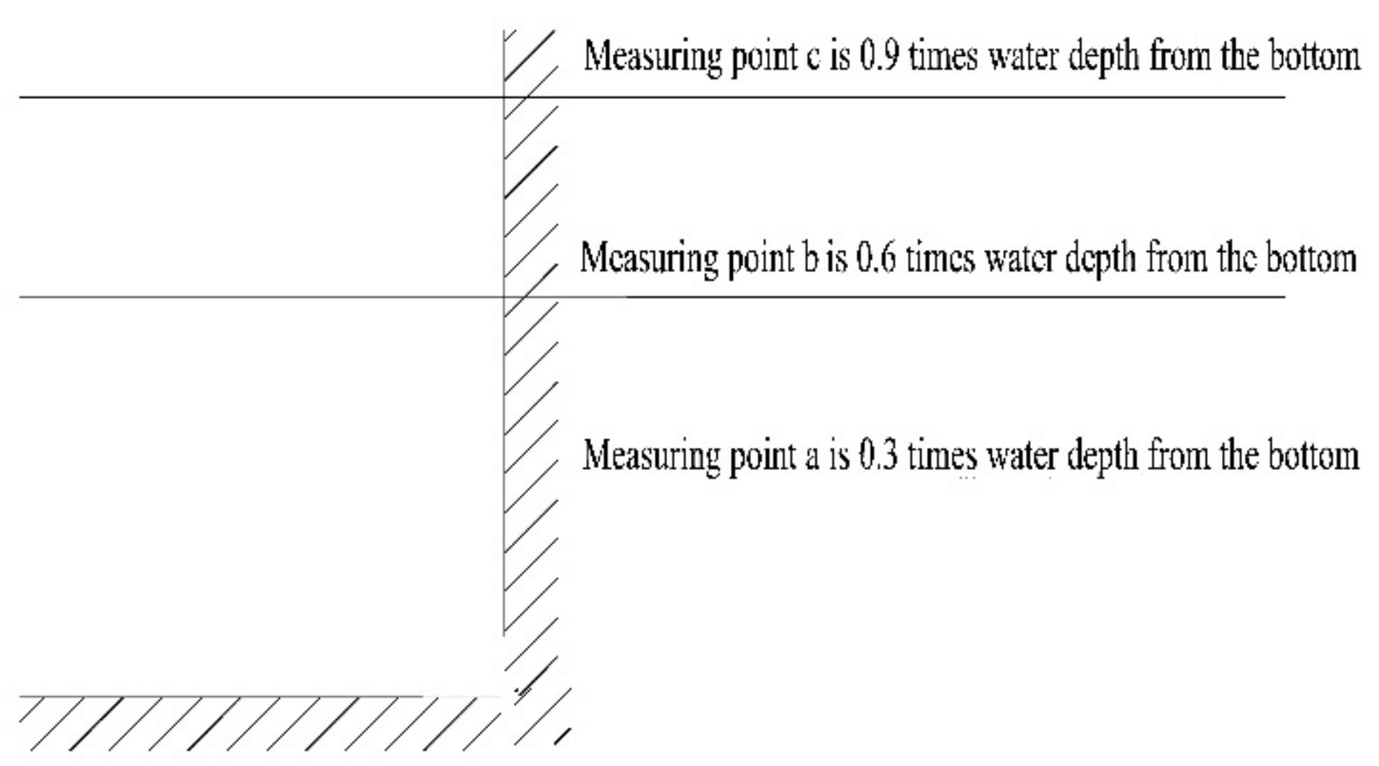
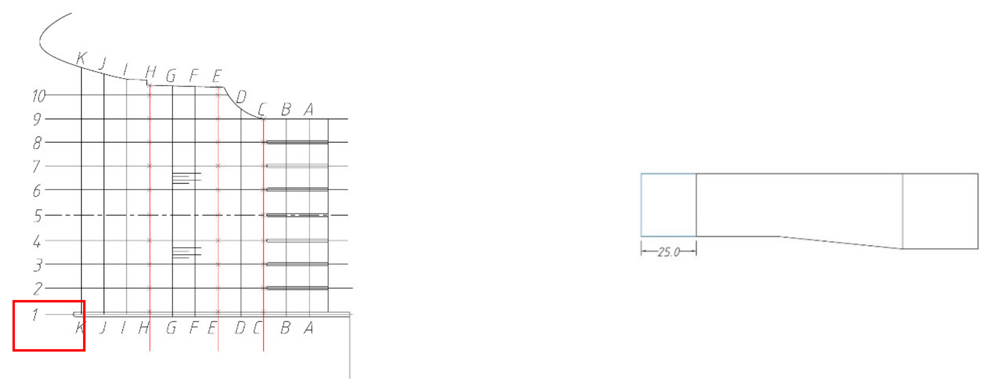
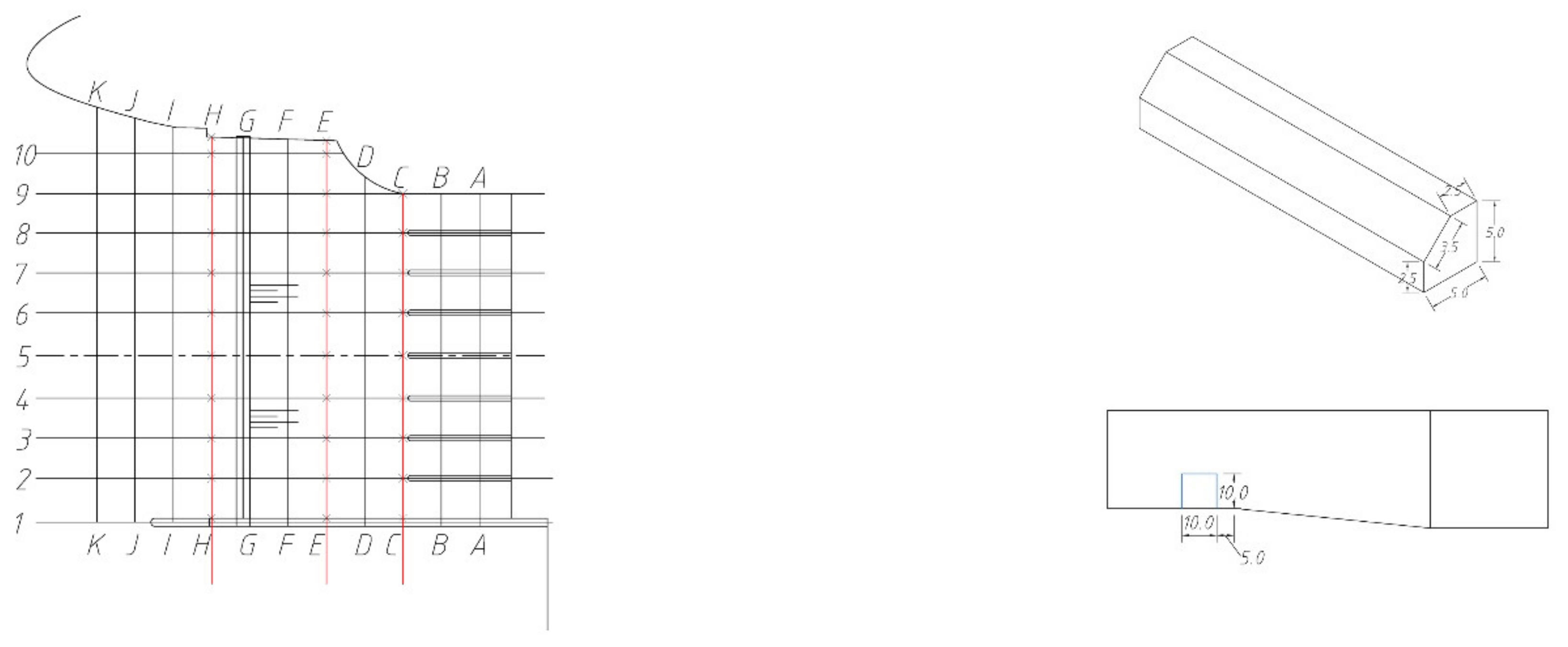
In order to quantitatively compare the influence of rectification measures on the flow pattern of intake water, the velocity distribution of three sections (C, E, H) in the intake forebay of the pumping station is determined in the calculation. The position of the section is shown in the Figure. With the reference [24] method, 8–10 measuring lines were arranged in each section, and the position is shown in Figure 6; in this Figure, 5.00 and 3.30 are the bottom elevation of the forebay, and 1.1 is the slope. Three measuring points were taken for each line, 0.3 h, 0.6 h, and 0.9 h, respectively, where h is water depth. The location of measuring points is shown in Figure 7.
4.3. Rectification Plan
During the simulation process, several plans were compared, such as a diversion wall, a sill, a rectifier pier, a side opening of the diversion wall, etc., as well as combination plans, such as the combination of a rectifier sill and a pier, the combination of a rectifier sill and a side opening of the diversion wall, etc. The main plans are shown in Table 3.
5. Results and Discussion
5.1. Flow Pattern Comparison of the Model Test and Numerical Simulation
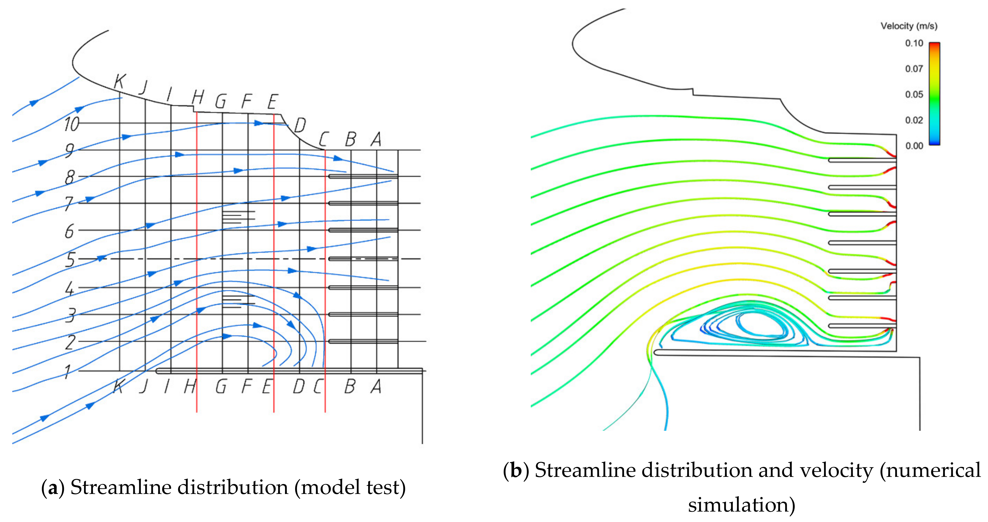
5.1.1. Original Plan
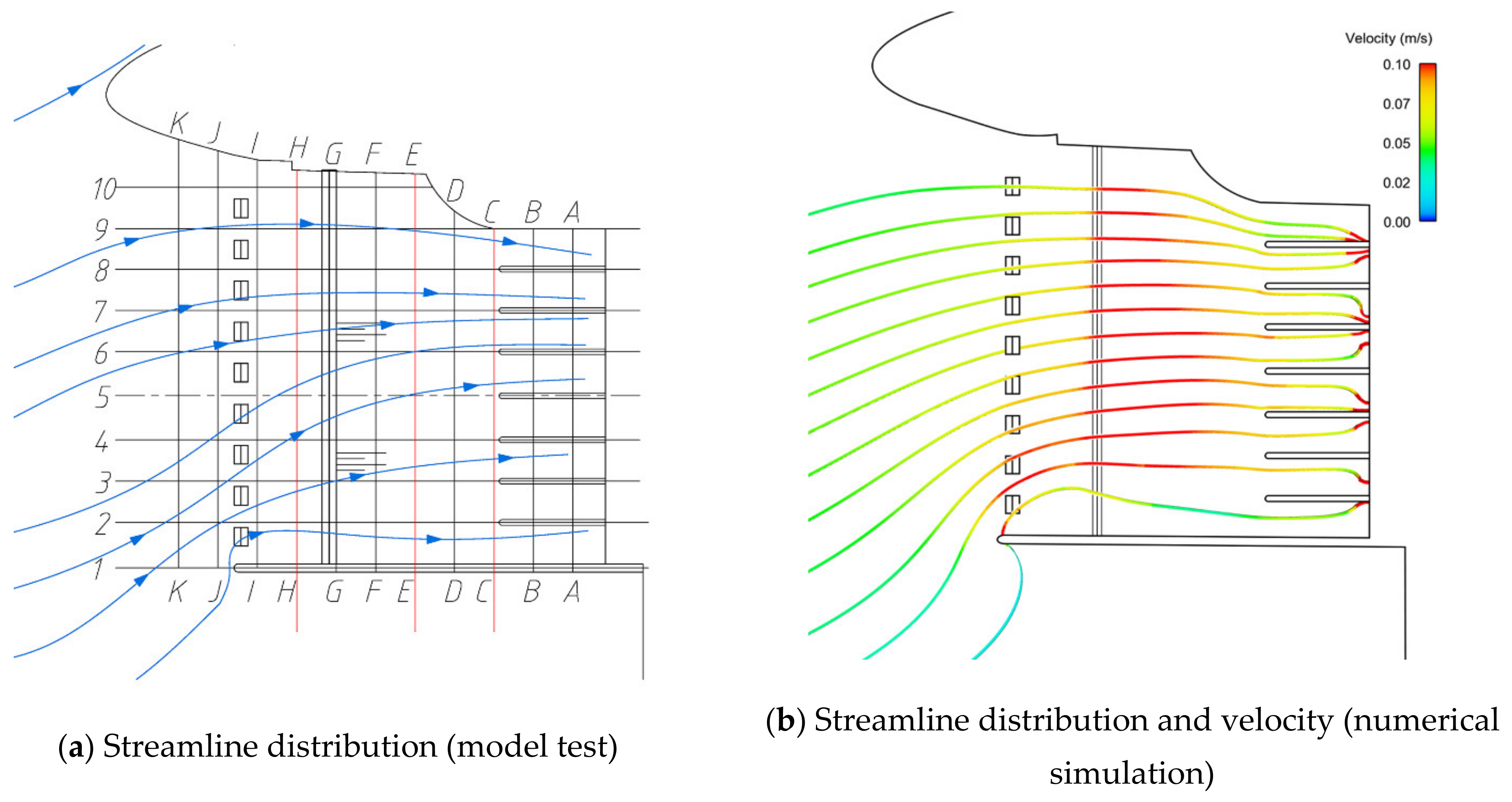
Model test and numerical simulation flowchart for the design operating water level are presented in Figure 14, while the model test and numerical simulation flowchart for the flood control water level are presented in Figure 15. The main flow in the forebay of the Exi River drainage pumping station deflects, and the main flow deflects to the left bank of the forebay. A large range of vortexes appear in the right bank area of the forebay, which is unfavorable for the efficient, safe, and reliable operation of #1 and #2. According to the calculation of sections C, E, and H of the forebay, with the flow of water, the uniformity of flow velocity from section H to section C first decreases and then increases. Potentially, the velocity distribution of water flow at section E is the smallest, indicating that the velocity distribution of water flow at section E is the most uneven.
5.1.2. Extended Diversion Wall
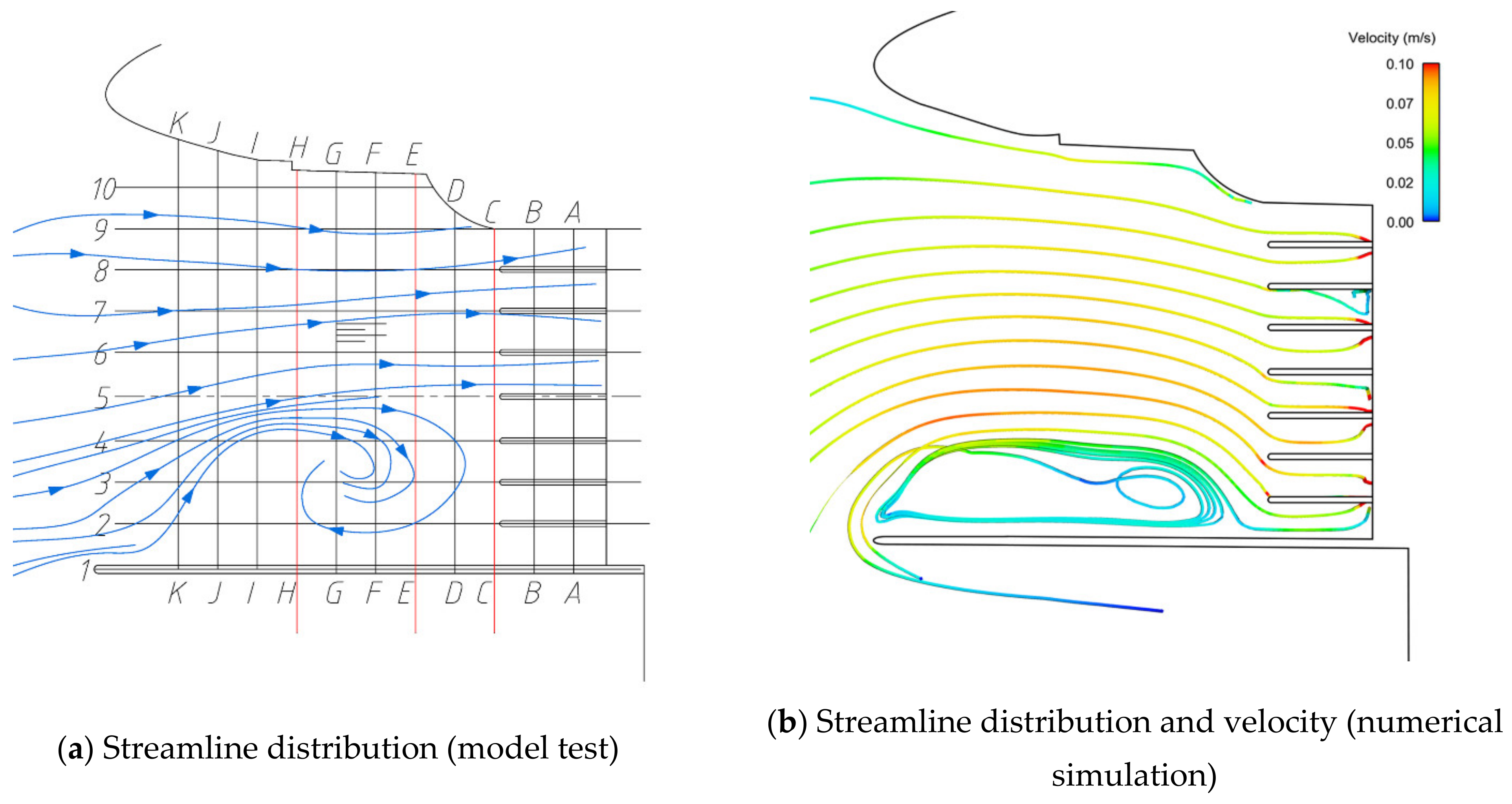
At the design operating level, after the diversion wall was lengthened by 7.5 m (Figure 16), the vortex still existed and formed a narrow vortex in the right bank area of the front pool, which was still not conducive to the overall stable operation of the pumping station. After further lengthening the diversion wall to 15 m (Figure 17), the vortex still existed and was even larger, forming a narrow vortex in the right bank area of the front pool, and the water flow was biased towards the left bank area of the front pool, which was still not conducive to the overall stable operation of the pumping station. Compared with the original scheme, the uniformity of flow velocity decreases in sections C, E, and H, indicating that the flow velocity distribution is more inhomogeneous in this scheme compared with the original scheme.
5.1.3. Rectifier Sill
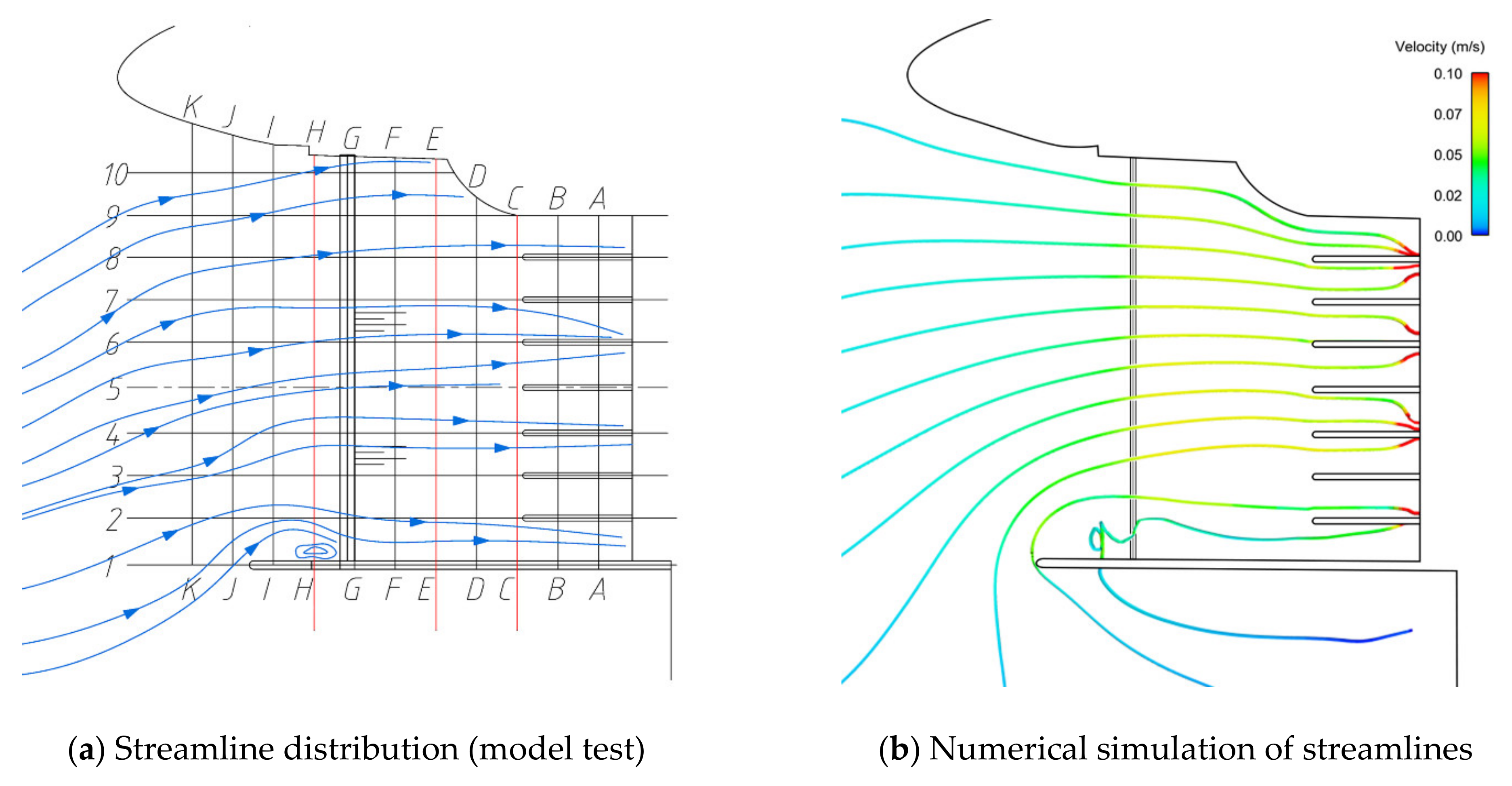
The rectifier sill is added as a rectifying measure (Figure 18). Because the water flow on the backside of the sill whirls and produces a small vortex area [25,26], once the water flows through the sill, it forms a constant vortex [27] due to the separation of water flow so as to achieve the purpose of energy dissipation and improvement of the flow pattern. Under the design operating conditions, the flow pattern of the forebay is obviously improved and the vortex on the right bank of the original forebay disappears by setting a rectifier at the entrance section of the forebay.
5.1.4. Rectifier Sill and Pier
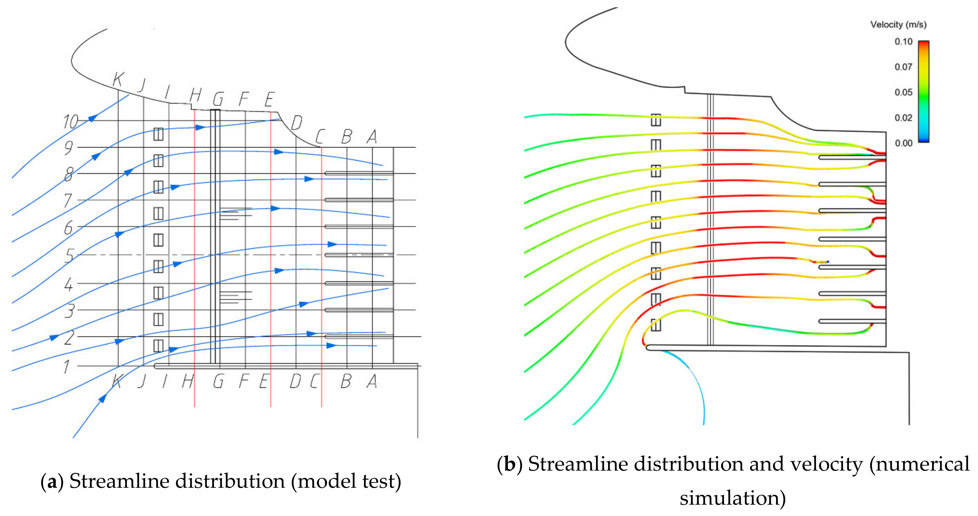
On the basis of improving the flow pattern of the rectifier sill, we tried to further increase the rectifier pier to improve the flow pattern. A row of rectifier piers is arranged at the front section of the diversion wall, and the test and numerical simulation calculation were carried out under four working conditions: the lowest operating water level, the design operating water level, the highest operating water level, and the flood control water level.
The results show that the flow pattern of the forebay is obviously improved under the conditions of the minimum operating water level (Figure 19), the design operating water level (Figure 20), the maximum operating water level (Figure 21), and the high flood control water level (Figure 22), and the vortex area on the right bank of the forebay disappears. Compared with the original plan, the velocity uniformity decreases in Section C and E, but increases in section H, which indicates that the velocity uniformity is improved far away from the inlet of the pumping station, but it is still uneven near the pumping station.
5.1.5. Rectifier Sill and Diversion Wall Opening
In addition to the traditional rectification methods such as rectifier sill and piers, this paper provides a variety of solutions for the flow pattern of the forebay, referring to the literature [28] which studies the influence of geometric parameters of orifices in the diversion pier on the rectification pattern of the forebay. The orifice in the diversion pier can reduce the return area near the diversion pier and improve the uniformity of flow velocity distribution of the flow channel. Because the water level ratio inside the forebay after unit startup first reduces, the force on both sides of the diversion wall is uneven, and the opening of the diversion wall can balance the water pressure. Therefore, two types of opening sizes of the diversion wall are proposed in this paper, and the design operating conditions are numerically simulated.
The diversion wall features 6 × 6 m side holes near the bottom and forms a small-scale swirl in the right bank area of the forebay (Figure 23).
The diversion wall features 3 × 3 m side holes near the bottom. The water flow is relatively smooth as a whole and the flow rate is uniform. Only small low-speed vortexes appear at the side holes (Figure 24).
The results show that the flow pattern in plan 7 is relatively smooth and the uniformity of flow velocity is 5.5%, 6.2%, and 20.2% higher in sections C, E, and H than in the original plan, respectively. The uniformity of flow velocity is improved significantly.
5.2. Quantitative Analysis of Hydraulic Performance Parameters of the Forebay
To quantitatively check the rectification effect of the rectification measures, the axial velocity distribution uniformity of the C, E, and H sections of the intake forebay of the Exi River drainage station was carried out under the design operating conditions. The calculation formula [29] is as follows:
where is the axial velocity of the ith grid unit, m/s; is the average axial flow rate in the overflow section, m/s; is the area of the eleventh grid unit, m2; n is the total number of grid cells in the overflow section.
The calculation results are shown in Table 4.
It can be seen from the analysis that the closer the water intake is, the more uniform the velocity distribution is. Because the vortex and the return flow mainly exist in the middle of the forebay, and the slope there is 1:10, the velocity uniformity of section E significantly decreases. After rectification, the flow field structure changes are more complex. Due to the increase of the diversion wall, the velocity uniformity of the three sections becomes worse in plans 2 and 3. The velocity uniformity of section H of plans 4 and 5 with a better rectification effect is slightly higher than that of the original plan. The velocity uniformity of sections 6 and 7 with a better rectification effect is higher than that of the original plan, and that of section C near the pumping station side is 4% higher than that of the original plan. The H section away from pumping station side is raised by 14%.
To further quantitatively measure the eddy suppression effect of rectification measures under the design operating conditions, the eddy areas of plans 1–7 were compared and the parameter ratio w of the eddy area and the reduction rate Δw of the eddy area were introduced. The calculation formulas are as follows:
where is the vortex area in plan I, m; is the forebay area, in this model, it is 2.092 m2.
The calculation results are shown in Table 5. The vortex elimination effect of plan 2 is limited, and plan 3 even increases the vortex. Plans 4 and 5 have the best vortex elimination effect, which is more than 90%. Plans 6 and 7 have the best vortex elimination effect, which is more than 85%.
5.3. The Best Plan
In conclusion, it can be seen that the effect of plan 7 is the best. Besides, compared with the original plan and plan 7, the axial velocity of the measuring point in the water depth of 0.6 h at section E was selected for comparison, and the ideal average velocity, , was calculated by Equation (16):
where is the mass flow, m3/s; is the flow area of section E, m2.
The results are shown in Figure 25. X is a dimensionless number referring to the relative position, ; l is the pumping station inlet width, m; x is the coordinate of the measurement point with the central axis as the origin, m.
The deviation from the ideal average velocity of each measuring point in plan 7 is smaller, which is significantly better than in the original plan, indicating that the velocity uniformity of the measuring points on the measuring line is better.
6. Conclusions
The improvement of the pumping station flow pattern can effectively improve the operating performance of pumps, reduce sedimentation, improve the reliability and economy of the pumping station, reduce costs, and improve efficiency. In this paper, the research method of the combined physical model test and the VOF CFD model (Flow-3D) was used to propose different optimization schemes. In order to optimize the flow pattern of the inlet front pool, various rectification measures were tried in front of the pumping station, including five rectification measures of lengthening the flow guide wall, arranging the rectification can, the combination of a rectification can and a rectifier pier, and the combination of a rectification can and an open hole flow guide wall. The flow patterns of the five optimized measures were simulated by model tests, and the flow patterns, flow uniformity of characteristic sections, and swirl area of the five optimized measures were calculated using numerical simulations. The results of model tests and numerical simulations were comprehensively compared.
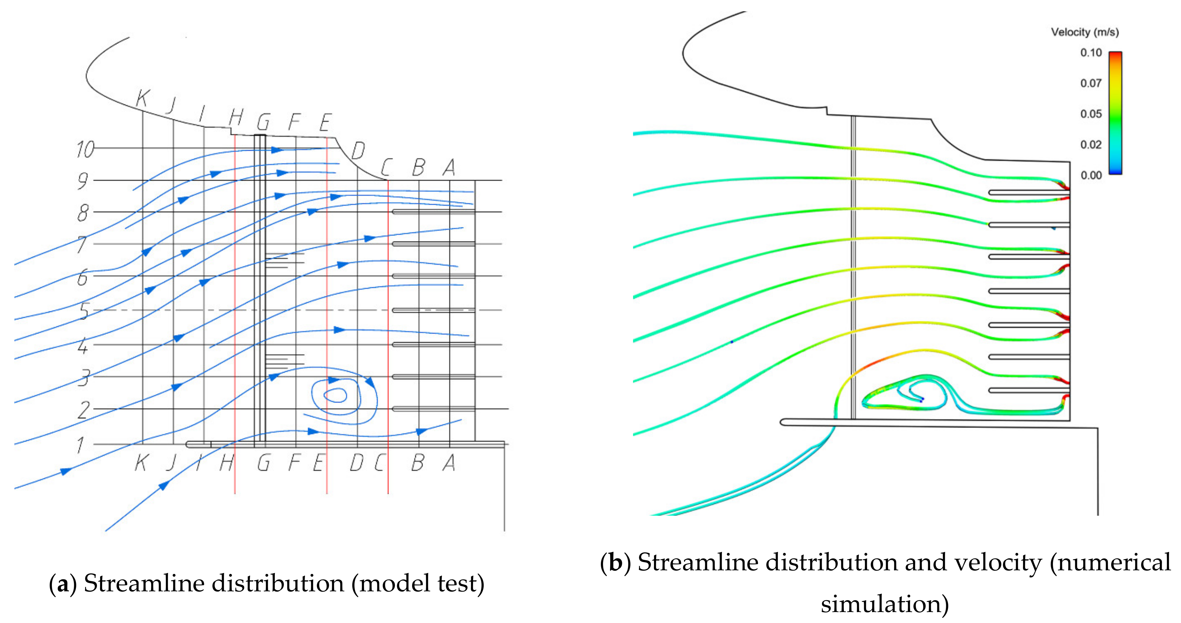
(1) In the absence of any engineering measures (Figure 14 and Figure 15), the flow pattern of the forebay of the pumping station is more complex, and there is a large vortex area that accounts for more than 13% of the total area of the forebay, which is easy to cause the siltation of the river channel and the intake tank, which will increase the impact of water flow on the safe and economic operation of the pumping station.
(2) In plans 2 and 3, the extended diversion wall (Figure 16 and Figure 17) can reduce the velocity uniformity of the test section, but cannot improve the flow pattern and reduce the vortex. In plan 3, the vortex area even increases by 25%, which has a negative effect, so it is not recommended to adopt this plan.
(3) In plan 4, only the rectifier sill (Figure 18) is adopted, which can effectively improve the flow pattern and eliminate the vortex. In plan 5, the combination of a rectifier sill and rectifier piers (Figure 19, Figure 20, Figure 21 and Figure 22) is used as the flow regime control measure of the forebay of the pumping station. After two rectifying measures, the vortex of the forebay can be effectively reduced by more than 90%, so that the water can flow smoothly into the pumping station.
Author Contributions
Conceptualization, F.Y.; software and writing—original draft preparation, Y.Z.; writing—review and editing, F.Y. and Y.J.; experiments, T.W.; Investigation, Y.Z. and D.J.; supervision, C.L.; All authors have read and agreed to the published version of the manuscript.
Funding
This research was funded by the National Natural Science Foundation of China (grant No. 51609210), major projects of the Natural Science Foundation of the Jiangsu Higher Education Institutions of China (grant No. 20KJA570001), the open research subject of the Key Laboratory of Fluid and Power Machinery, Ministry of Education (szjj2016-078), the Science and Technology Plan Project of the Yangzhou City (grant No. YZU201901), the Technology Project of the Water Resources Department of the Jiangsu Province (grant No. 2020029), and the Priority Academic Program Development of the Jiangsu Higher Education Institutions (PAPD).
Institutional Review Board Statement
Not applicable.
Informed Consent Statement
Not applicable.
Data Availability Statement
All data necessary to carry out the work in this paper are included in the figures, tables or are available in the cited references.
Conflicts of Interest
The authors declare no conflict of interest.
References
- Li, Q.; Xu, J.; Li, D.; Li, N. Development and Prospect of Irrigation and Drainage Pump Stations in China. China Rural Water Hydropower 2015, 12, 6–10. [Google Scholar]
- Zhang, J.; Lu, Z. Discussion on Type Selection and Application of Pumping Station. China Water Wastewater 2016, 32, 38–40. [Google Scholar]
- Xu, C.D.; Wang, R.R.; Liu, H.; Zhang, R.; Wang, M.Y.; Wang, Y. Flow pattern and anti-silt measures of straight-edge forebay in large pump stations. Int. J. Heat Technol. 2018, 36, 1130–1139. [Google Scholar] [CrossRef]
- Wang, F.; Tang, X.; Chen, X.; Xiao, R.; Yao, Z.; Yang, W. A review on flow analysis method for pumping stations. J. Hydraul. Eng. 2018, 49, 47–61, 71. [Google Scholar]
- Xu, C.; Zhang, H.; Zhang, X.; Han, L.; Wang, R.; Wen, Q.; Ding, L. Numerical simulation of the impact of unit commitment optimization and divergence angle on the flow pattern of forebay. Int. J. Heat Technol. 2015, 33, 91–96. [Google Scholar] [CrossRef]
- Li, C.; Chao, L. Hydraulic performance of pump sumps based on CFD approach. J. Hohai Univ. (Nat. Sci.) 2009, 37, 52–56. [Google Scholar]
- Zhou, J.; Zhong, Z.; Liang, J.; Shi, X. Three-dimensional Numerical Simulation of Side-intake Forebay of Pumping Station. J. Irrig. Drain. 2015, 34, 52–55. [Google Scholar]
- Can, L.; Chao, L. Numerical simulation and improvement of side-intake characteristics of multi-unit pumping station. J. Hydroelectr. Eng. 2015, 34, 207–214. [Google Scholar]
- Xia, C.; Cheng, L.; Zhao, G.; Yu, L.; Wu, M.; Xu, W. Numerical simulation of flow pattern in forebay of pump station with single row of square columns. Adv. Sci. Technol. Water Resour. 2017, 37, 53–58. [Google Scholar]
- Luo, J.; Lin, Y. Hydraulic test of pump sumps of thermal (nuclear) power plants. J. Hohai Univ. 2000, 28, 106–110. [Google Scholar]
- Constantinescu, G.; Patel, V. Role of turbulence model in prediction of pump-bay vortices. J. Hydraul. Eng. 2000, 126, 387–391. [Google Scholar] [CrossRef]
- Kadam, P.; Chavan, D. CFD analysis of flow in pump sump to check suitability for better performance of pump. Int. J. Mech. Eng. Robot. 2013, 1, 56–65. [Google Scholar]
- Song, W.; Pang, Y.; Shi, X.; Xu, Q. Study on the Rectification of Forebay in Pumping Station. Math. Probl. Eng. 2018, 2018, 2876980. [Google Scholar] [CrossRef]
- Muller, C.J.; Craig, I.K. Energy reduction for a dual circuit cooling water system using advanced regulatory control. Appl. Energy 2016, 171, 287–295. [Google Scholar] [CrossRef] [Green Version]
- Caishui, H. Three-dimensional numerical analysis of flow pattern in pressure forebay of hydropower station. Procedia Eng. 2012, 28, 128–135. [Google Scholar] [CrossRef]
- Zhan, J.M.; Wang, B.C.; Yu, L.H.; Li, Y.; Ling, T. Numerical investigation of flow patterns in different pump intake systems. J. Hydrodyn. Ser. B 2012, 24, 873–882. [Google Scholar] [CrossRef]
- Wang, F. Computational Fluid Dynamics Analysis: Principle and Application of CFD Software; Tsinghua University: Beijing, China, 2004; pp. 7–11. [Google Scholar]
- Wang, F. The Analysis of Computational Fluid Dynamics-CFD Software Theory and Application; Tsinghua University Press: Beijing, China, 2004. [Google Scholar]
- Roache, P.J. Quantification of uncertainty in computational fluid dynamics. Annu. Rev. Fluid Mech. 1997, 29, 123–160. [Google Scholar] [CrossRef] [Green Version]
- Savage, B.M.; Crookston, B.M.; Paxson, G.S. Physical and numerical modeling of large headwater ratios for a 15 labyrinth spillway. J. Hydraul. Eng. 2016, 142, 04016046. [Google Scholar] [CrossRef]
- Liu, H.; Liu, M.; Bai, Y.; Du, H.; Dong, L. Grid convergence based on GCI for centrifugal pump. J. Jiangsu Univ. (Nat. Sci. Ed.) 2014, 35, 279–283. [Google Scholar]
- Wang, S.S.; Roache, P.J.; Schmalz, R.A., Jr.; Jia, Y.; Smith, P.E. (Eds.) Verification and Validation of 3D Free-Surface Flow Models; American Society of Civil Engineers: Reston, VA, USA, 2008. [Google Scholar] [CrossRef]
- Yabing, D. Numerical Simulation Study on the Scheme of Trajecmtory Bucket Type Energy Dissipation for Overflow Sam of Shiziya Reservoir; Xi’an University of Technology: Xi’an, China, 2018. [Google Scholar]
- Zhao, Z. Hydrometry; The Yellow River Water Conservancy Press: Zhengzhou, China, 2005. [Google Scholar]
- Jiren, C.L.L.C.Z.; Fangping, T. Numerical Simulation of Turbulent Flow around Sill with RNG k-ε Turbulent Model. J. Trans. Chin. Soc. Agric. Mach. 2005, 3, 37–39. [Google Scholar]
- Haiying, X. Comparison of simulation effect of turbulence model upon flow passing on sill. J. Water Resour. Water Eng. 2012, 23, 163–165. [Google Scholar]
- Feng, X. Flow analysis of bottom sill rectification and back sill of pump station forebay. Jiangsu Water Resour. 1998, 26, 31–33, 38. [Google Scholar]
- Xu, B.; Gao, C.; Xia, H.; Lu, W. Influence of Geometric Parameters of Perforated Diversion Pier on Flow-rectifying Effect in Forebay of Sluice-pump Station Project. J. Yangtze River Sci. Res. Inst. 2019, 36, 58–62. [Google Scholar]
- Fan, Y.; Chuanliu, X.; Chao, L.; Yao, Y.; Lijian, S. Influence of axial-flow pumping system operating conditions on hydraulic performance of elbow inlet conduit. Trans. Chin. Soc. Agric. Mach. 2016, 47, 15–21. [Google Scholar]
Figure 1.
Analysis flowchart.

Figure 2.
Satellite image of the Exi River flood discharge station.

Figure 3.
General layout of the test and the local model diagram of the forebay.

Figure 4.
3D model of the numerical simulation area.

Figure 5.
Head loss with different mesh quantities.

Figure 6.
Diagram of line arrangement.

Figure 7.
Schematic diagram of measuring point positions.

Figure 8.
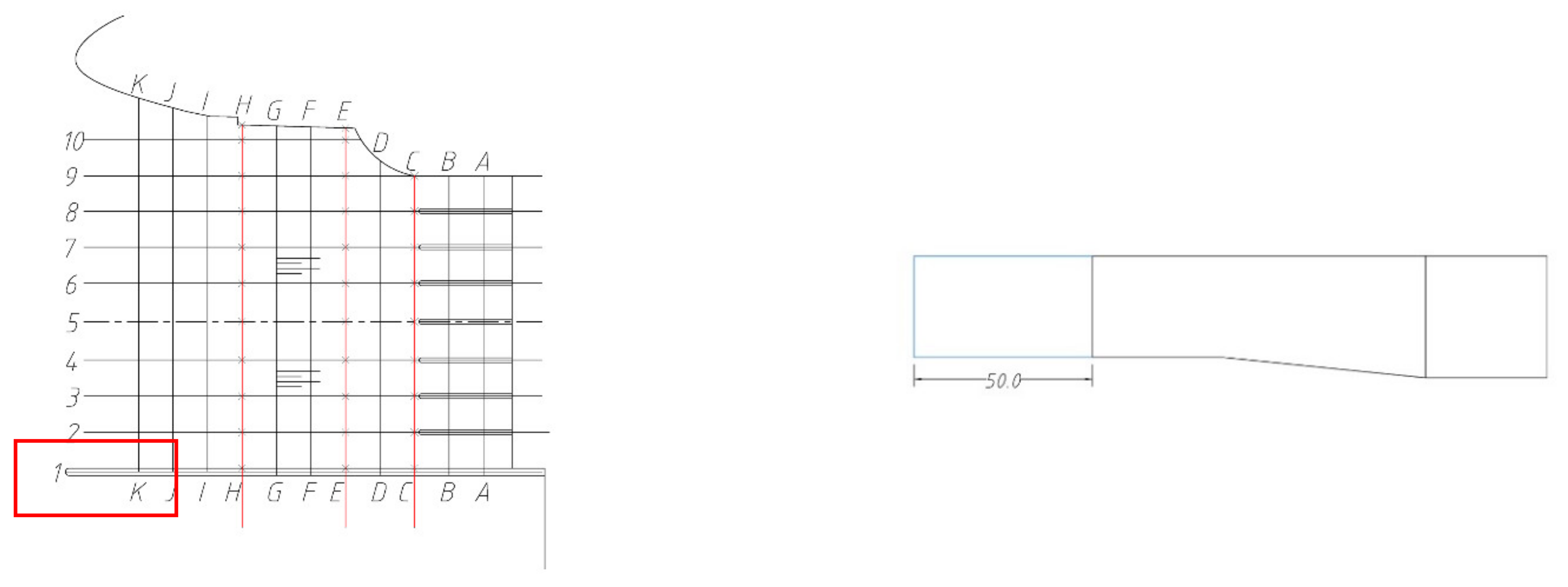
Plan 2 (unit: cm).

Figure 9.
Plan 3 (unit: cm).

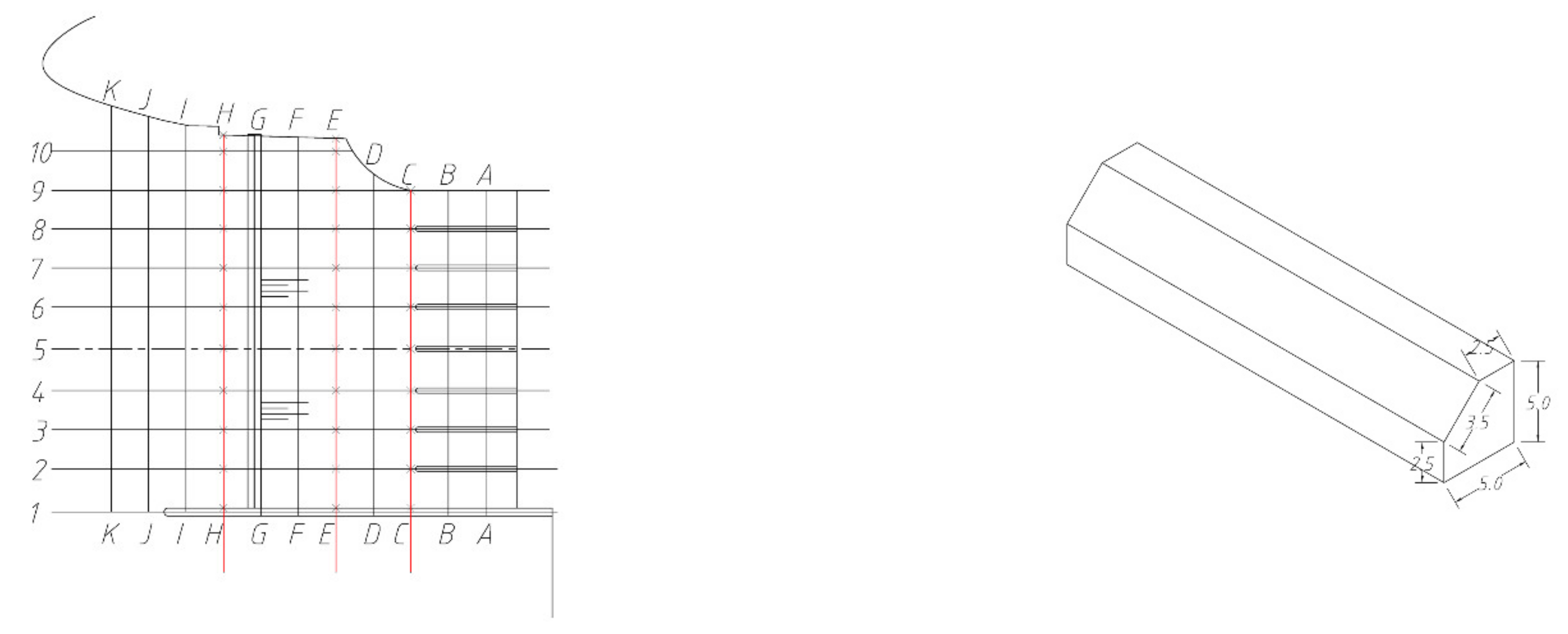
Figure 10.
Plan 4 (unit: cm).

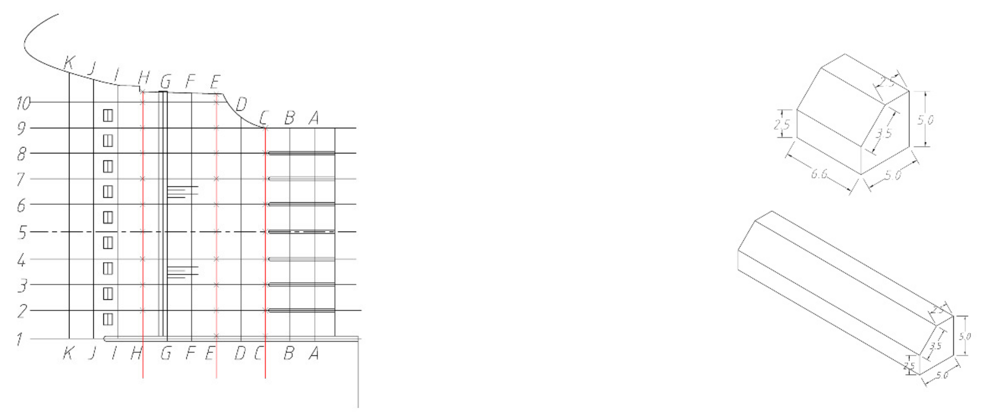
Figure 11.
Plan 5 (unit: cm).

Figure 12.
Plan 6 (unit: cm).

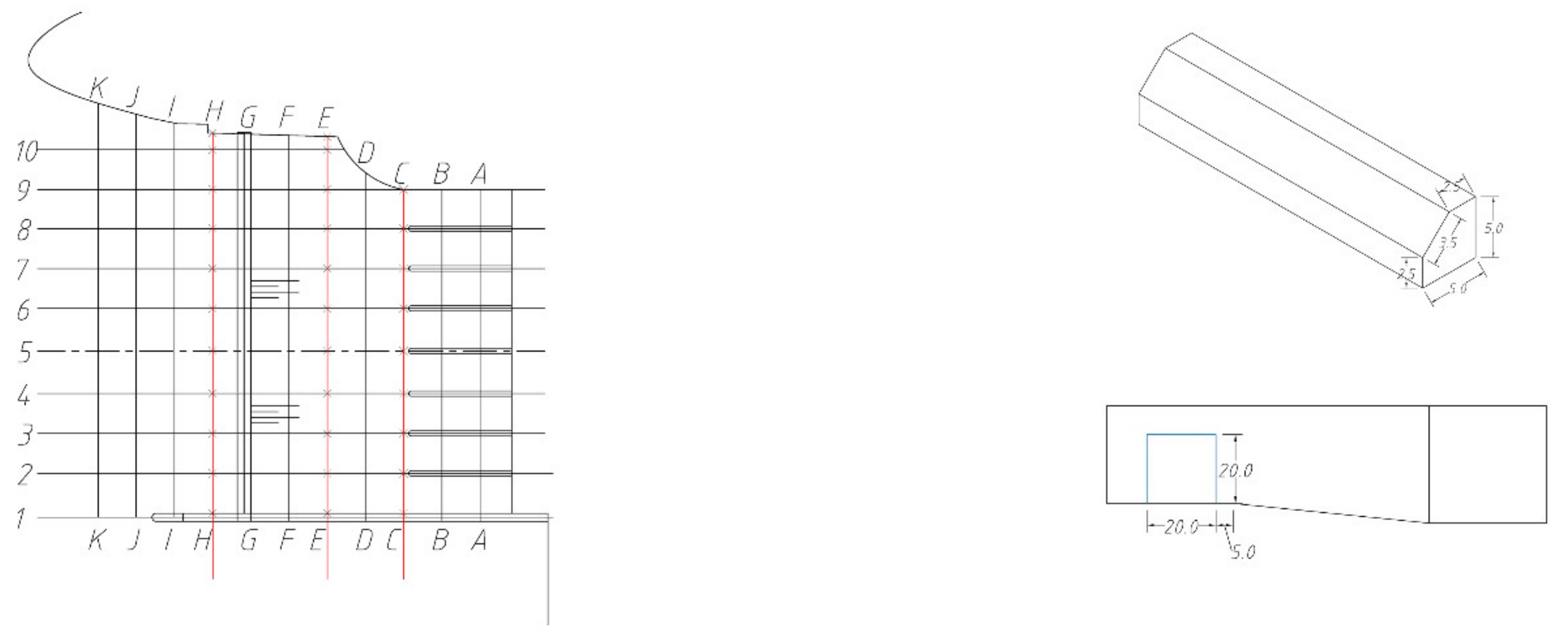
Figure 13.
Plan 7 (unit: cm).

Figure 14.
Plan 1 (design operating water level).

Figure 15.
Plan 1 (flood control water level).

Figure 16.
Plan 2 (design operating water level).

Figure 17.
Plan 3 (design operating water level).

Figure 18.
Plan 4 (design operating water level).

Figure 19.
Plan 5 (minimum operating water level).

Figure 20.
Plan 5 (design operating water level).

Figure 21.
Plan 5 (maximum operating water level).

Figure 22.
Plan 5 (flood control water level).

Figure 23.
Plan 6 (design operating water level).

Figure 24.
Plan 7 (design operating water level).

Figure 25.
Plan 1 and 7 velocity at point b, section E.


Table 1.
Characteristic water level table.
| Characteristic Water Level | Upper Reaches/m | Lower Reaches/m | Net Head/m |
|---|---|---|---|
| Minimum operating water level | 9.00 | 10.00 | 1.00 |
| Design operating water level | 10.00 | 12.06 | 2.06 |
| Maximum operating water level | 12.47 | 14.11 | 1.64 |
| Flood control water level | 13.09 | 14.11 | 1.02 |
Table 2.
GCI calculation result.
| Mesh Size (m) | Total Number of Meshes | r (Dk/Dk+1) | p | Q(m3/s) | ||
|---|---|---|---|---|---|---|
| 0.03 | 767,646 | 0.02100 | ||||
| 0.025 | 1,320,405 | 1.20 | 1 | 0.02115 | 0.00714 | 4.46519 |
| 0.02 | 2,467,681 | 1.25 | 1 | 0.02113 | 0.00094 | 0.47039 |
Table 3.
List of test plans for flow pattern of the pumping station.
| Plan Number | Plan Description | Action Description (Prototype in Parentheses) |
|---|---|---|
| 1 | Original plan | No rectification measures |
| 2 | Diversion wall | The diversion wall is lengthened by 25 cm (7.5 m). The shape and arrangement of rectification measures are shown in Figure 8. |
| 3 | Diversion wall | The diversion wall is lengthened by 50 cm (15 m). The shape and arrangement of rectification measures are shown in Figure 9. |
| 4 | Rectifier sill | The bottom width of the sill is 5 cm (1.5 m), the top width is 2.5 cm (0.75 m), and the top elevation is 5 cm (1.5 m). The shape and arrangement of rectification measures are shown in Figure 10. |
| 5 | Rectifier sill and pier | The width of the rectifier pier bottom is 5 cm (1.5 m), top width is 2.5 cm (0.75 m), crest elevation is 5 cm (1.5 m), and length is 6.67 cm (2 m). The shape and arrangement of rectification measures are shown in Figure 11. |
| 6 | Rectifier sill and side opening of diversion wall | The side hole of the diversion wall is 20 × 20 cm (6 × 6 m). The shape and arrangement of rectification measures are shown in Figure 12. |
| 7 | Rectifier sill and side opening of diversion wall | The side hole of the diversion wall is 10 × 10 cm (3 × 3 m). The shape and arrangement of rectification measures are shown in Figure 13. |
Table 4.
Section velocity uniformity.
| Plan Number | Velocity Distribution Uniformity Vu+ (%) | ||
|---|---|---|---|
| C | E | H | |
| 1 | 78.22 | 60.23 | 68.67 |
| 2 | 76.33 | 63.32 | 59.3 |
| 3 | 77.69 | 53.75 | 58.53 |
| 4 | 76.01 | 56.40 | 70.43 |
| 5 | 79.11 | 54.79 | 70.89 |
| 6 | 80.78 | 63.59 | 87.95 |
| 7 | 82.55 | 63.97 | 82.61 |
Table 5.
Vortex parameters of each plan.
| Plan Number | Vortex Area (m2) | Area Ratio (%) | Reduction Rate (%) |
|---|---|---|---|
| 1 | 0.284 | 13.590 | — |
| 2 | 0.099 | 4.742 | 65.107 |
| 3 | 0.358 | 17.113 | −25.923 |
| 4 | 0.004 | 0.167 | 98.769 |
| 5 | 0.004 | 0.177 | 98.699 |
| 6 | 0.039 | 1.883 | 86.141 |
| 7 | 0.022 | 1.033 | 92.402 |
Publisher’s Note: MDPI stays neutral with regard to jurisdictional claims in published maps and institutional affiliations. |
© 2021 by the authors. Licensee MDPI, Basel, Switzerland. This article is an open access article distributed under the terms and conditions of the Creative Commons Attribution (CC BY) license (https://creativecommons.org/licenses/by/4.0/).
Share and Cite
MDPI and ACS Style
Yang, F.; Zhang, Y.; Liu, C.; Wang, T.; Jiang, D.; Jin, Y. Numerical and Experimental Investigations of Flow Pattern and Anti-Vortex Measures of Forebay in a Multi-Unit Pumping Station. Water 2021, 13, 935. https://doi.org/10.3390/w13070935
AMA Style
Yang F, Zhang Y, Liu C, Wang T, Jiang D, Jin Y. Numerical and Experimental Investigations of Flow Pattern and Anti-Vortex Measures of Forebay in a Multi-Unit Pumping Station. Water. 2021; 13(7):935. https://doi.org/10.3390/w13070935
Chicago/Turabian StyleYang, Fan, Yiqi Zhang, Chao Liu, Tieli Wang, Dongjin Jiang, and Yan Jin. 2021. "Numerical and Experimental Investigations of Flow Pattern and Anti-Vortex Measures of Forebay in a Multi-Unit Pumping Station" Water 13, no. 7: 935. https://doi.org/10.3390/w13070935
Note that from the first issue of 2016, this journal uses article numbers instead of page numbers. See further details here.