
Evaluating the Performance of Sentinel-1A and Sentinel-2 in Small Waterbody Mapping over Urban and Mountainous Regions


1
Key Laboratory of Agricultural Big Data, Ministry of Agriculture and Rural Affairs, Beijing 100081, China
2
Key Lab of Guangdong for Utilization of Remote Sensing and Geographical Information System, Guangdong Open Laboratory of Geospatial Information Technology and Application, Research Center of Guangdong Province for Engineering Technology Application of Remote Sensing Big Data, Guangzhou Institute of Geography, Guangdong Academy of Sciences, Guangzhou 510070, China
3
Agricultural Information Institute, Chinese Academy of Agricultural Sciences, Beijing 100081, China
*
Author to whom correspondence should be addressed.
Water 2021, 13(7), 945; https://doi.org/10.3390/w13070945
Submission received: 28 January 2021
/
Revised: 16 March 2021
/
Accepted: 25 March 2021
/
Published: 30 March 2021
(This article belongs to the Section Hydrology)
Abstract
:Accurate waterbody mapping can support water-related environment monitoring and resource management. The Sentinel series satellites provide high-quality Synthetic Aperture Radar (SAR) and optical observations that are commonly used in waterbody mapping. However, owing to the 10-m spatial resolution of Sentinel data, previous studies mostly focused on the mapping of large waterbodies. In this work, we evaluated the performance of small waterbody mapping over urban and mountainous regions with two datasets, the average annual VH backscatter coefficients (VHavg), derived from the Sentinel-1A series, and the Modified Normalized Difference Water Index (MNDWI), derived from cloud-free Sentinel-2. A proven framework of waterbody mapping based on watershed segmentation and noise reduction was employed to assess the performance of the two datasets in waterbody identification. The validation was performed by comparing their results with 1-m spatial resolution reference waterbody data. Assessment metrics, including Precision, Recall, and F-measure, were employed. Results showed that: (1) the MNDWI outperformed the VHavg by 9 percentage points of the F-measure; (2) there was more room for results of VHavg to improve the accuracy through a combination with noise reduction; and (3) the potential smallest identifiable waterbody area (recall rate larger than 0.8) was larger than 104 m2.
Keywords:
Guangzhou; MNDWI; Sentinel-1A; Sentinel-2; waterbody; watershed segmentation; small waterbody1. Introduction
Surface waterbodies, including rivers, channels, ponds, lakes, and reservoirs, play an essential role in socioeconomic development and ecosystem balance, and provide irreplaceable natural resources for humans’ survival and development [1,2]. The waterbodies in Guangzhou City, an important central city in China with a permanent population of 15.31 million at the end of 2019, are under intensive pressure because of human activities (e.g., housing development, dredging, and agricultural pollution) or natural phenomena (e.g., extreme weather). To better understand waterbody changes and to allow comprehensive water-related studies and planning activities, such as water resource management and water disaster prevention, it is critical to conduct waterbody mapping [3].
Remote sensing is a powerful tool for measuring and monitoring waterbody dynamics. In the past several decades, numerous satellite sensors capable of waterbody mapping were launched. The remotely sensed data can be divided into two categories based on their imaging principles. (1) Optical remote sensing is a passive technique that relies on solar illumination. Commonly used bands are visible, near infra-red (NIR), and short-wave infrared (SWIR) wavelengths. The typical optical data sources include Landsat-5/7/8 [4], Sentinel-2 [5], and GF-1/2 [6,7]. Waterbody mappings have been conducted on a single band, multiple bands, and water indices. Specifically, the water index-based method combines two or more spectral bands using various algebraic operations to enhance the discrepancy between the waterbody and land [8,9]. (2) Synthetic Aperture Radar (SAR) is an active remote sensing technique that uses microwave electromagnetic energy to form complex images of terrain reflectivity. Waterbody mappings with SAR data are based on the value of SAR backscatter coefficients. The typical SAR data sources include Envisat [10], Radarsat-2 [11], and Sentinel-1 [12,13]. Comparing the two data sources, optical images are simple to interpret as they are closer to human vision. However, SAR images are relatively difficult to interpret as the data may vary depending upon many factors, including the incidence angle, terrain structure, and surface roughness.
Compared with other land covers, waterbodies are significant as they generally appear as dark objects in either optical or SAR images. Several methods have been proven effective for both data sources in waterbody mapping, including thresholding [9], supervised/unsupervised classification [14,15], image segmentation [4], and deep learning [16]. However, regardless of the method used, there is a limit to the size of the waterbody that can be identified as the performance of the method is constrained by the spatial resolution of images. Under ideal conditions, such as flat terrain and homogeneous land covers, the smallest identifiable waterbody may be close to the image resolution because waterbodies and land have significant spectral differences. However, when the ground conditions are complex, the waterbody mapping performance is significantly reduced as the small waterbody may be easily confused with multiple types of noise. In this paper, noise is defined as an object with similar image values to those of waterbodies in a remote sensing image [17]. The typical sources of noise and their features are described below.
- (1)
- Cloud/cloud shadows: SAR images are free of cloud-related contamination. However, the optical images are easily affected by clouds and cloud shadows. Thus, it is necessary to select cloudless images through visual or automatic methods [18].
- (2)
- Mountain/built-up shadows: The mountain/skyscraper shadow is caused by similar factors as optical and SAR images: An object blocks the path of direct radiation in optical imaging and the radar beam in the case of SAR. However, unlike optical imagery, in which objects in shadows can be seen because of atmospheric scattering, there is no information in a SAR shadow because there is no return signal. Theoretically, the mountain shadow can be identified by simulating hill-shading with Digital Elevation Models (DEMs) and the solar azimuth and elevation at the time of image acquisition. However, owing to the limitation of DEM resolution and the influence of land cover, using DEM alone is often not enough to eliminate mountain shadows in practice. Thus, ancillary data other than DEM are required.
- (3)
- Flat surfaces: Noises like those made by asphalt, cement surfaces, and roads mainly appear in SAR images rather than in optical images. Generally, the rough surfaces scatter the energy and return a significant amount back to the antenna, resulting in a bright feature. In contrast, the flat surfaces reflect the signal away, resulting in a dark feature. As waterbodies absorb radar energy, they also exhibit a dark feature. Flat surfaces are often misidentified as waterbodies by using images of SAR backscatter coefficients. However, these noises are usually different from waterbodies in infrared bands of optical data.
- (4)
- Ships: The ships have a high reflectivity or backscatter coefficient that may cause “holes” in the waterbody extraction results.
The dense time series of Sentinel offers a unique opportunity to systematically monitor waterbodies by both optical and SAR measurements with similar features, including fine spatial resolution (approximately 10 m), frequent revisit (12 days for Sentinel-1A, 5 days for Sentinel-2 A/B together), and accessibility.
Previous studies mostly focused on the mapping of large waterbodies. It is not clear how effective Sentinel data are in small waterbody mappings over urban and mountainous regions, where multiple types of noise exist. It is necessary to analyze the waterbodies’ pixel values in images to determine the capabilities and limitations of Sentinel data in waterbody identification. In this study, we defined the smallest identifiable waterbody area level as the first time the Recall rate at this waterbody area level reached a threshold of 0.8.
This study attempted to answer three questions: (1) What is the difference in the waterbody identification performance between Sentinel-1 and Sentinel-2 data? (2) How much improvement can some classic noise reduction methods bring to the accuracy of waterbody identification? (3) For urban and mountainous regions, how large is the smallest identifiable waterbody for Sentinel data at a 10-m resolution? The remainder of this article is organized as follows. Section 2 describes the experimental materials, a previously developed framework of waterbody mapping, and assessment metrics. Section 3 presents the analysis of the experimental results. Section 4 provides the discussion. Conclusions and future research are given in Section 5.
2. Materials and Methods
2.1. Study Area
The study area was Guangzhou City, China. The total area of the study region is 7434.4 km2. The topography of Guangzhou is mountainous and densely covered with waterways. The terrain heights decrease from north to south. The highest peak has an elevation of 1210 m. The northeast is a moderately mountainous area; the middle is a hilly basin; and the south is a coastal floodplain, a component of the Pearl River Delta [19,20]. According to the Guangzhou Water Resources Bulletin of 2018, the total waterbody area was estimated at 744 km2, which accounted for 10.05% of the city’s total land area [21].
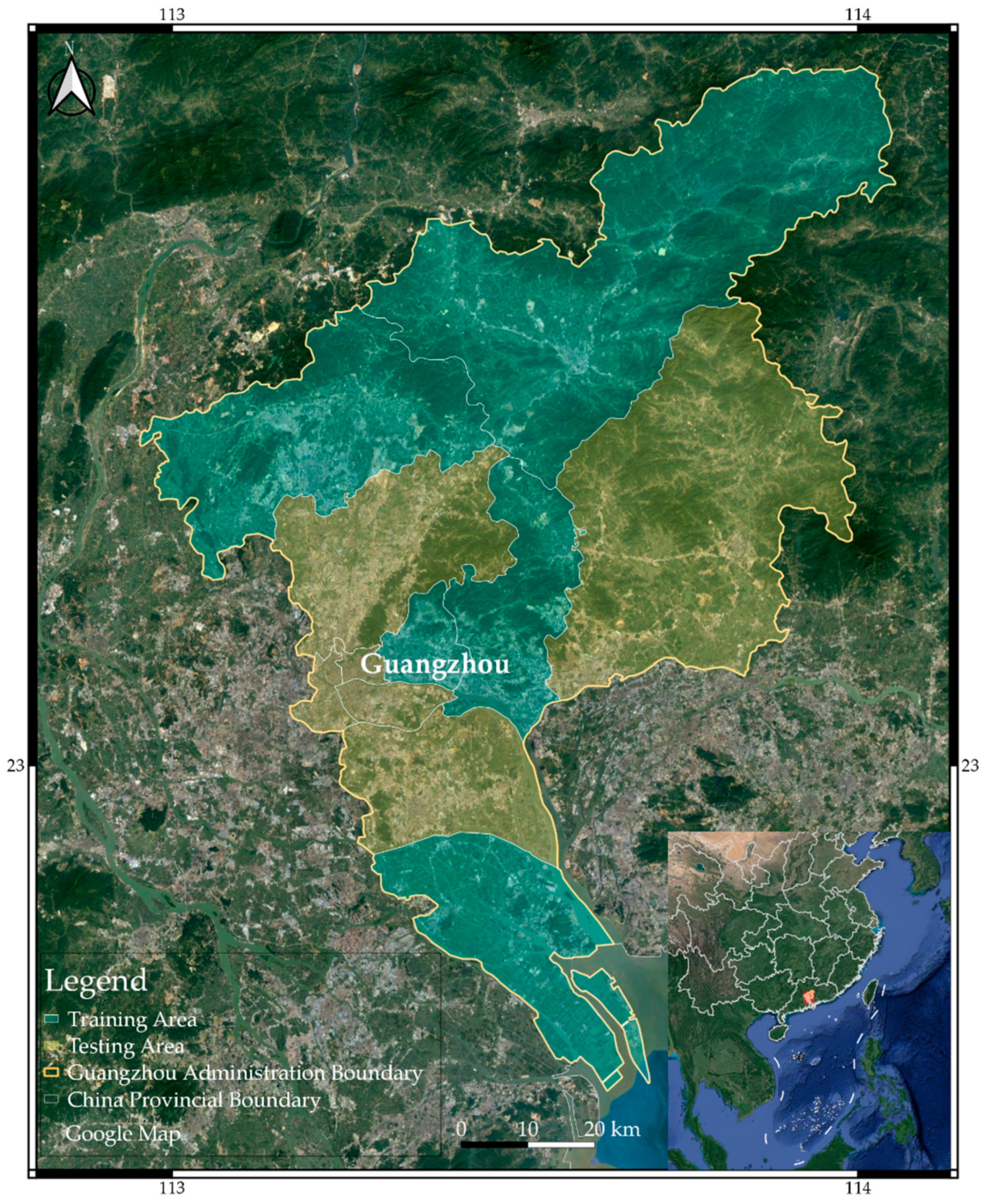
The extent of the study area is presented in Figure 1. The yellow area was chosen as the training area, and the green area was the testing area.
2.2. Data
For this study, three imagery data sources, Sentinel-1A (S1A), Sentinel-2 (S2), and SRTM DEM, were chosen for waterbody mapping and result pruning. The data and preprocessing details are described below.
2.2.1. Sentinel-1A Data and Pre-Processing
The S1A interferometric wide swath (IW) GRD product has a 12-day revisiting period. Thus, each location covers 30 to 31 images per year. Among the entire study area, 421 images in 2017 were downloaded from the European Space Agency (ESA) Sentinels Scientific Data Hub website (https://scihub.copernicus.eu/dhus, accessed on 25 March 2021). The S1A product contains both VH and VV polarization, but only VH polarization was selected for waterbody mapping.
The S1A data were preprocessed using the Sentinel Application Platform (SNAP) toolbox (version 6.0.0). The preprocessing stages included: (1) radiometric calibration using the export image band as the sigma naught band (σ°), (2) ortho-rectification using range Doppler terrain correction with the Shuttle Radar Topography Mission (SRTM) Digital Elevation Model (DEM), (3) re-projection to Sinusoidal projection, World Geodetic System (WGS) 84, and resampling to a spatial resolution of 10 m using the bilinear interpolation method, (4) calculation of the average composite of annual VH σ° band time series using Equations (1) and (5) conversion of the sigma naught band from linear backscatter units to logarithmic decibels (dB) [22].
where is VH σ° band time series per year.
2.2.2. Sentinel-2 Data and Pre-Processing
The Sentinel-2 data used in this study were derived using the Sentinel-2A&B L1C product, which was already rectified through radiometric and geometric corrections [23]. The product was downloaded via the Sentinel-2 repository on the Amazon Simple Storage Service (registry.opendata.aws/sentinel-2, accessed on 25 March 2021). Four indices were calculated from Sentinel-2 data, MNDWI (Modified Normalized Difference Water Index), NDBI (Normalized Difference Built-up Index), NDVI (Normalized Difference Vegetation Index), and NDVImax using Equation (2) to Equation (5):
where ρgreen, ρred, ρNIR, and ρSWIR1 are the visible green, red, near-infrared, and short-wave infrared bands in S2 data, and NDVIannual is the NDVI time series per year. The ρSWIR1 band with a 20-m spatial resolution was resampled to 10 m to match the other bands using the bilinear interpolation method.
2.2.3. Shuttle Radar Topography Mission (SRTM) Digital Elevation Model (DEM)
The topographic SLOPE data were produced from the SRTM DEM product with 1-arcsecond (nearly 30 m) spatial resolution and then resampled to 10 m to match the Sentinel data using the bilinear interpolation method.
2.2.4. Waterbody Reference Data
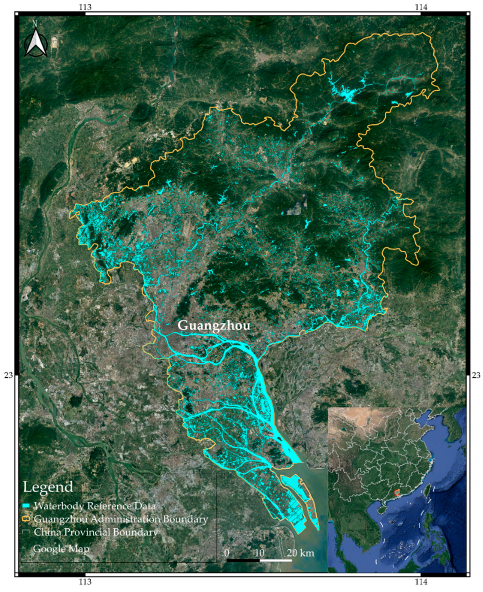
The waterbody reference data (WRD) of Guangzhou City were manually delineated according to high-resolution optical images of Google Maps and Bing Maps from 2017 to 2019 (Figure 2). Ubukawa [24] evaluated the position error of the two Maps in 10 cities around the world (including Shanghai, China) and found that the root mean square error (RMSE) for the satellite imagery represented in Google Maps and Bing Maps was 8.2 m and 7.9 m, respectively. This position error was less than the 10-m resolution of the Sentinel data, indicating that the data can verify the Sentinel data.
According to the reference data, there were 75,368 polygons of waterbodies, and the associated area was 656.63 km2. The size of the WRD was less than the estimated size in Guangzhou Water Resources Bulletin 2018 [21]. The possible reason was that some of the images used for WRD delineation were acquired in the dry season, and therefore part of the waterbodies failed to be extracted. Each waterbody was classified into one of five types: rivers, water ditches, reservoirs, lakes, and ponds. The details are shown in Table 1.
2.3. Framework of Waterbody Mapping
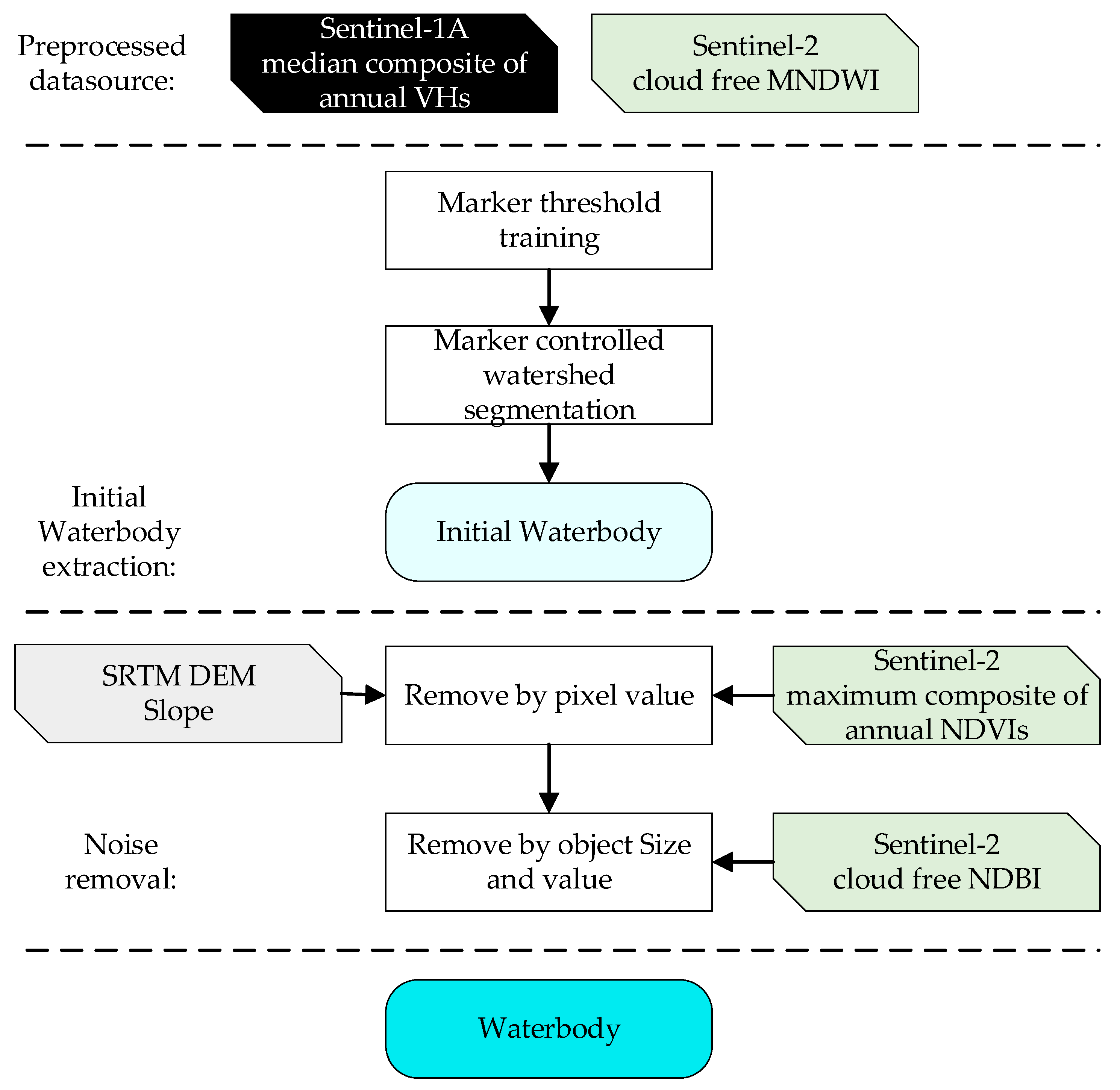
For a comparison of the performance of the S1A SAR and S2 optical datasets in waterbody extraction, we applied an automatic framework of waterbody extraction that was independent of the two datasets (Figure 3). The framework included two stages: the first was the initial waterbody extraction, which was adapted from existing methods [4]; the second was noise reduction, which was designed according to the characteristics of the study area.
2.3.1. Initial Waterbody Extraction
Previous studies suggested that marker-controlled watershed segmentation (MCW) is useful for waterbody mapping as it performs better in the edge position of waterbody compared with using a single threshold to distinguish a waterbody/non-water area [4]. A typical waterbody extraction process using MCW requires three steps: (1) Identifying the markers: For all pixels in the indices, including VHavg or MNDWI. The waterbody or non-water area with higher credibility is first marked; (2) Calculating the gradient of the indices: The indices are then applied with the Sobel operator to produce the gradient image, which is used to determine the boundaries between the markers of the waterbody and non-water area; and (3) Performing MCW: By using markers of the waterbody/non-water area and gradient of the indices, the MCW expands each marker iteratively until all unmarked pixels are marked as either waterbody or non-water.
In this method, the latter two steps are relatively fixed because there are no parameters involved. However, the markers in the first step are relatively sensitive to the segmentation result. As a result, the parameters that control the selection of markers require tuning.
We applied a thresholding method to produce the waterbody/non-water markers automatically. For each index, there were two thresholds associated with the typical value of the waterbody/non-water. Moreover, for each index, the statistics derived from WRD and images were applied to determine the two thresholds through Equations (6) and (7):
where , , , and are thresholds to identify waterbody/non-water with higher credibility in the VHavg and MNDWI indices, respectively. To determine the four thresholds, the WRD of the training area was applied to analyze the pixel values’ statistics for waterbody and non-water. The method was:
- (1)
- Generate the non-water polygons: The non-water (NW) polygons were generated using Equation (8).where PWRD and PNW are the polygons of WRD and NW, respectively. The Buffering3 and Buffering1 are buffers of the WRD data with 3 or 1 pixels, respectively.
- (2)
- Statistics on pixel values of waterbodies by each area level and non-water: For VHavg and MNDWI, we calculated the median of pixel values associated with NW data and WRD for each waterbody area level.
- (3)
- Determine the thresholds: We analyzed the statistical pixel values of WRD under different area levels and NW through a violin chart. Then, the values of , , , and were determined by those levels where the pixel values were changing rapidly. The details and results are described in Section 3.
At last, the initial waterbody mask (IWM) was extracted. However, the mask might contain a lot of noise at this stage, including mountain shadows, flat surfaces, and holes. Thus, a second stage of result pruning was required to correct and filter the IWM.
2.3.2. Noise Reduction
Three indices, SLOPE, NDVI, and NDBI, were involved in the noise reduction stage:
- (1)
- Mountain shadow removal by SLOPE: The SLOPE was first applied with the thresholding method to remove pixels in IWM that satisfied Equation (9). However, the use of slope data alone could not wholly exclude mountain shadows as the spatial resolution of SRTM DEM data was lower than that of the Sentinel data.
- (2)
- Mountain shadow removal by NDVImax: Mountain shadows are significant noise in waterbody identification. However, the mountains are usually covered by dense vegetation in southern China. Thus, it was possible to use the NDVImax that satisfied Equation (10) to eliminate mountain shadows.
- (3)
- Flat surface removal by NDBI: Waterbodies and flat surfaces have a similar SAR backscattering coefficient value. For optical data, these two types exhibit significant differences in the near-infrared and short-wave infrared bands. The NDBI was designed to identify built-up areas and barren land. Thus, Equation (11) was applied to distinguish between a waterbody and a flat surface.
- (4)
- Hole removal by binary image morphology: The waterbody extraction results may contain some “holes” caused by ships or islands. A binary image morphology method was thus applied to remove the holes. Additionally, a threshold satisfying Equation (12) was set on the maximum pixels of the holes to avoid holes caused by islands.
2.4. Accuracy Assessment
In this study, we defined “Accurate waterbody mapping” as mapping the actual distribution of waterbodies at a certain spatial resolution. This ensured that enough waterbodies were correctly identified and that the area of the water bodies was realistic. Thus, the accuracy of the extraction results was evaluated from two aspects: waterbody number and area.
The evaluation of the waterbody area was to calculate the identification rate of overall waterbody pixels. This helped us observe how the overall waterbody area was identified against the true waterbody area. This method is commonly used for the verification of waterbody mapping results [17,25]. However, these metrics may not be able to express the misidentification of small waterbodies, because the area of small waterbodies only accounts for a small part of the total area of waterbodies.
Therefore, we applied another verification method based on the waterbody number, which is to examine if the waterbody individuals are extracted correctly or falsely. To this end, if the proportion of correct identified pixels to total pixels for a waterbody of WRD is equal to or greater than 0.5, it is correctly extracted; otherwise, it is considered to be wrongly extracted. This helped us observe how many of the individual waterbodies were correctly identified. This method is commonly used for object identification [26]. In this method, each waterbody, regardless of its area, is considered as equally important.
For both evaluations, three metrics, Precision, Recall, and F-measure, were calculated by comparing the results with the WRD:
where true positive (TP) and false positive (FP) are correct and incorrect identifications, respectively. Note that the correct identification for evaluation of the waterbody number meant at least one pixel in a candidate waterbody had been detected. In the assessment of waterbody area, it signified that one pixel of an overall waterbody had been detected. False negative (FN) is the misidentification. Precision represents the probability that the identifications are valid. Recall is the probability that waterbodies were correctly identified, and F-measure is the harmonic mean of Precision and Recall.
3. Results
3.1. Statistics on the Waterbody Value in Images
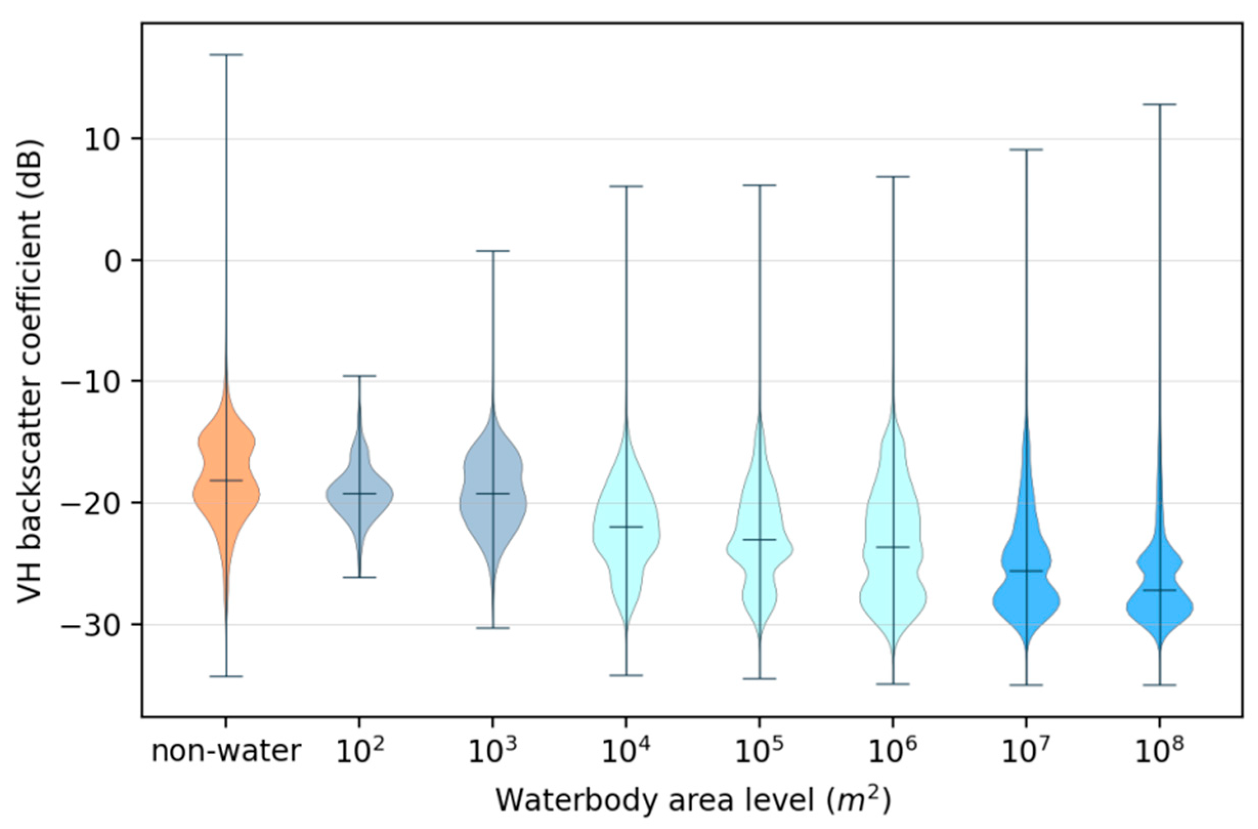
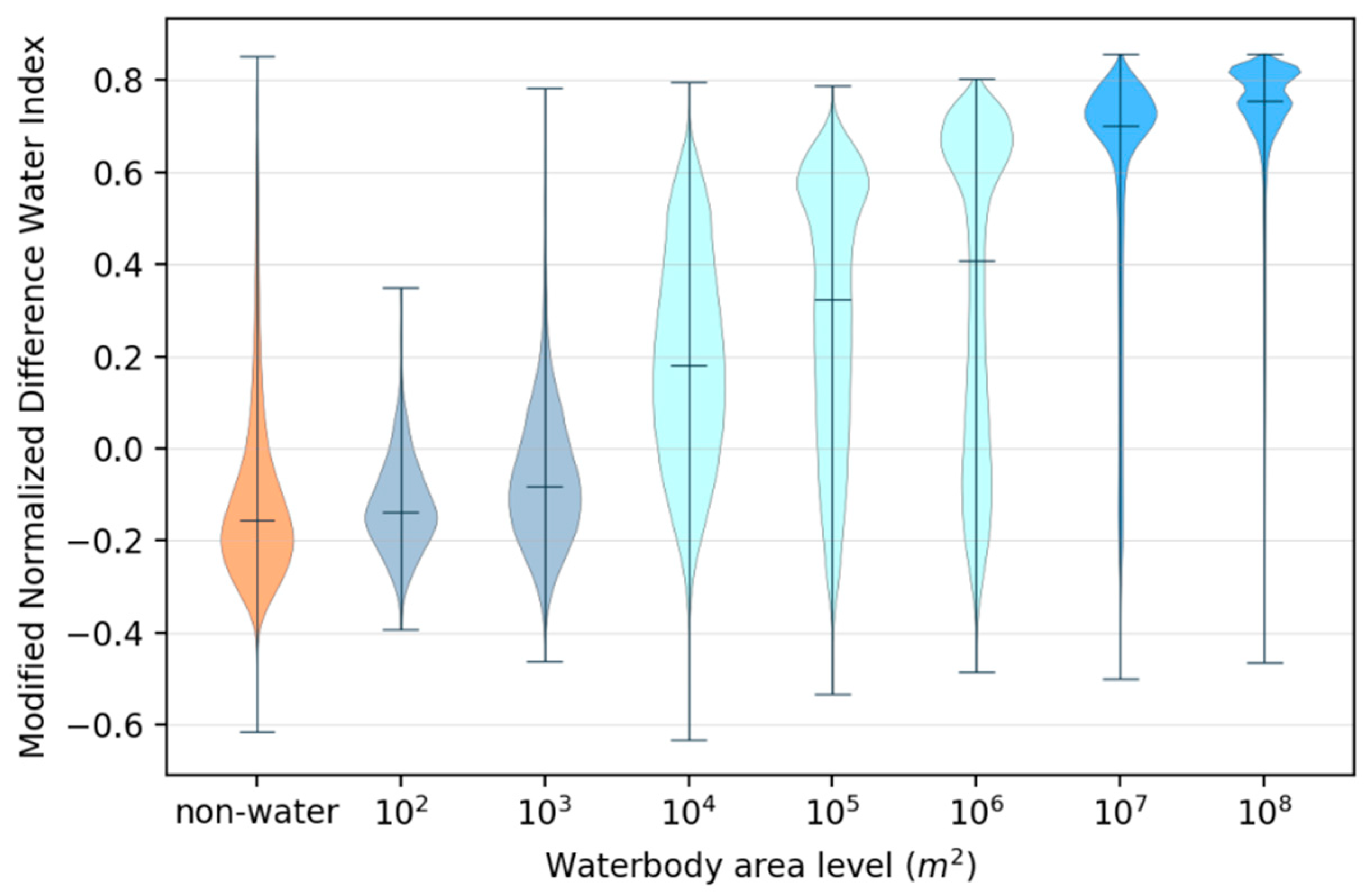
The distribution of VHavg and MNDWI according to waterbodies of different area sizes and non-water areas is shown in Figure 4 and Figure 5, respectively. We learned that the corresponding value of VHavg and MNDWI gradually diverged from the value of the non-water area as the waterbody area increased. For clarity, we divided all of the waterbodies according to their areas into three levels: small waterbodies (smaller than 103 m2), medium waterbodies (larger than 103 m2 but smaller than 106 m2), and large waterbodies (larger than 106 m2).
The median value of VHavg generally decreased as the waterbody’s area increased; for non-water, it was −18.07. For small waterbodies, the two median values were −19.20 and −19.18, which were very close to that of the non-water areas. For medium waterbodies, there were three bars with median values of −21.93, −22.94, and −23.55, respectively. For large waterbodies, it was lower than −25.58.
The median value of MNDWI increased as the waterbody’s area increased; for non-water, it was −0.16. For small waterbodies, the two median values were −0.14 and −0.08, which were very close to that of the non-water areas. For medium waterbodies, the three median values were 0.18, 0.32, and 0.40, respectively. For large waterbodies, it was higher than 0.70.
We found that the pixel values changed rapidly in two places. One was in the bar of 103 and 104. We defined the value of a high-confidence non-water area as the arithmetic mean of the median value of the two bars. The other was in the bar of 106 and 107. We defined the value of a high-confidence waterbody as the arithmetic mean of the median value of the two bars.
As a result, VHavg pixel values that were smaller than −24.56 or larger than −20.55 were marked as waterbodies/non-water areas. Similarly, the pixel value of MNDWI values larger than 0.55 or smaller than −0.05 was marked as waterbodies/non-water areas.
3.2. Accuracy of Waterbody Identification
The assessment of identification accuracy contained three parts:
(1) Accuracy of Waterbodies’ Total Area
Table 2 demonstrates that: (1) The noise reduction achieved a more significant improvement in VHavg than in MNDWI. Notably, comparing the results of noise reduced and initially extracted, for the VHavg dataset, the Precisiona improved by approximately 4 percentage points at the cost of lowering the Recalla by nearly 1 percentage point; and (2) The Recalla obtained by MNDWI was significantly higher than that of VHavg. Moreover, the F-measurea for VHavg and MNDWI were approximate 0.662 and 0.752, respectively.
(2) Accuracy of waterbody number
The results of the waterbody identification were derived from two datasets (VHavg and MNDWI) and two processing stages (initially extracted and noise-reduced). Several points were made, as shown in Table 3: (1) The noise reduction increased the Recalln and decreased the Precisionn as expected. Nevertheless, the highest Recalln value in the four sets of results was less than 0.27, indicating that a large number of small waterbodies have been misidentified. (2) The three metrics achieved using MNDWI were higher overall than those achieved using VHavg. (3) The F-measuren for both datasets were lower than 0.409.
(3) Recall rate by waterbody area level
We further tested the Recalln of the identified waterbodies against their area level. As Table 4 shows, the Recalln could also be divided into three levels: for small waterbodies, it was lower than 0.028; for medium waterbodies, it ranged from 0.167 to 0.847; and for large waterbodies, it was larger than 0.75. The situation was consistent with that of the training dataset. The table also shows that the SIWAL values for VHavg and MNDWI were larger than 107 and 104 m2, respectively.
4. Discussion
4.1. Noise Reduction
Comparing the noise reduction results with those of the initially extracted results of both VHavg and MNDWI, the noise reduction increased Precisiona and Precisionn and deceased Recalla and Recalln. However, the changes in the last three metrics were only around 1 percentage point. This was because the noise reduction method’s thresholds were relatively loose and had a small effect on the results. The only exception was that the Precisiona for VHavg increased by 4 percentage points. Thus, it can be inferred that there was some large area of noise introduced. After checking the results, we found that the major misidentifications were caused by reasons that included mountain shadows, artificial facilities, and ships.
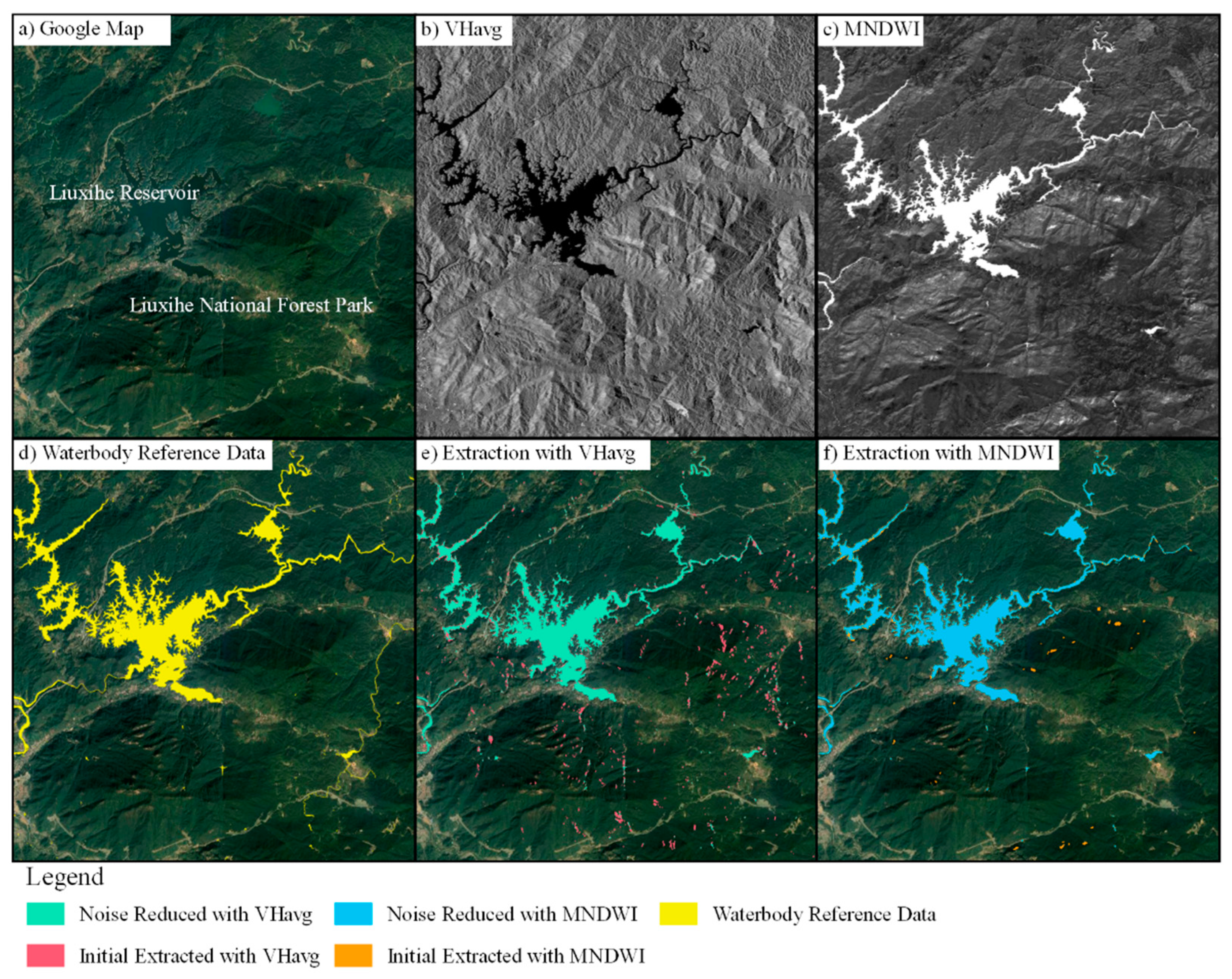
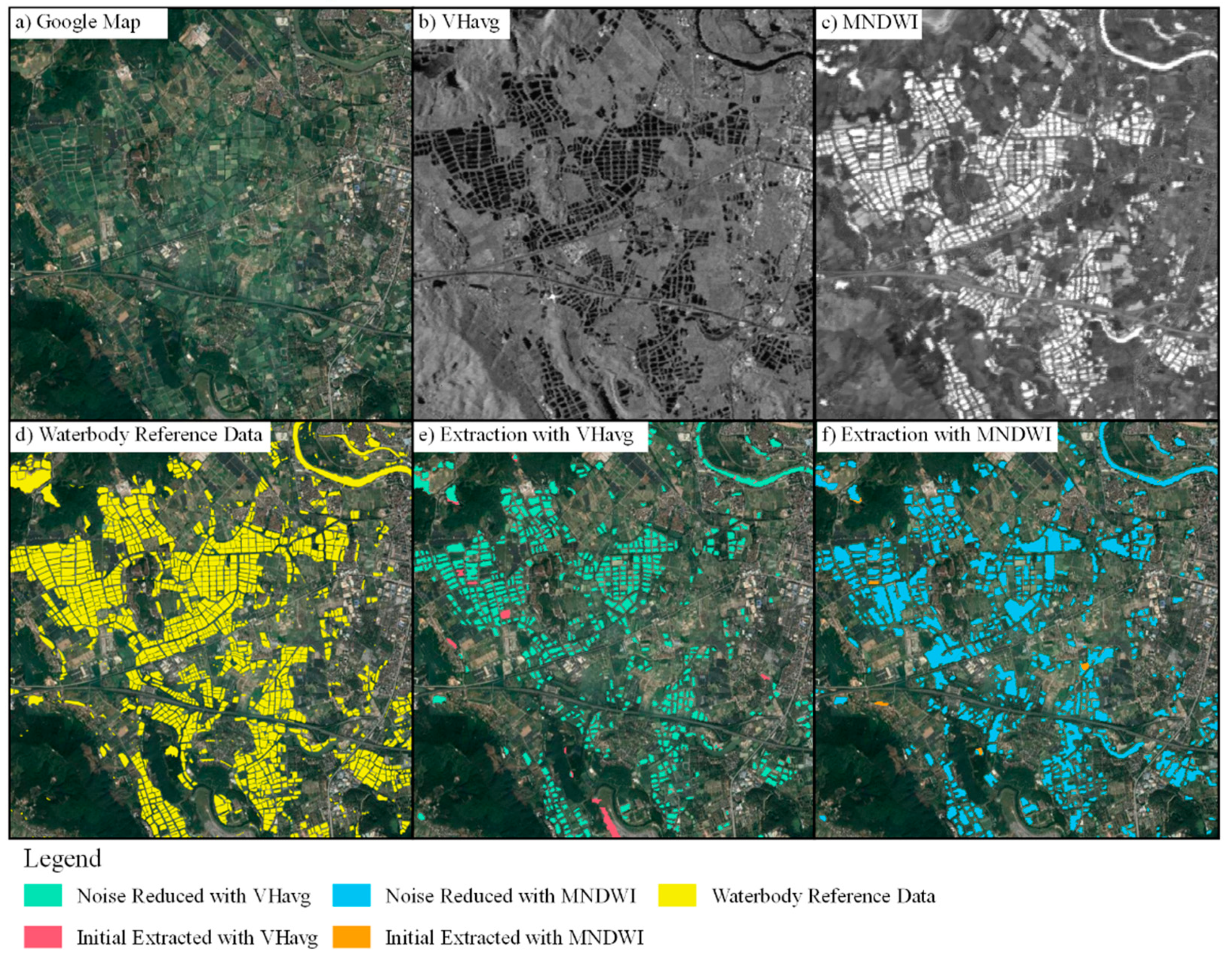
Figure 6 shows a typical case of mountain shadows denoising. The terrain in this area is quite undulating. For example, the altitude of the Liuxihe Reservoir is only 160 m. However, the altitude of the adjacent Liuxihe National Forest Park reaches 1000 m. In this case, the VHavg (Figure 6e) generated significantly more noises than MNDWI (Figure 6f). However, SAR is an active remote sensing device, which does not rely on sunlight. Moreover, SAR data are vulnerable to shadowing effects from steep mountains because of the side-looking viewing geometry of SAR satellite sensors [12].
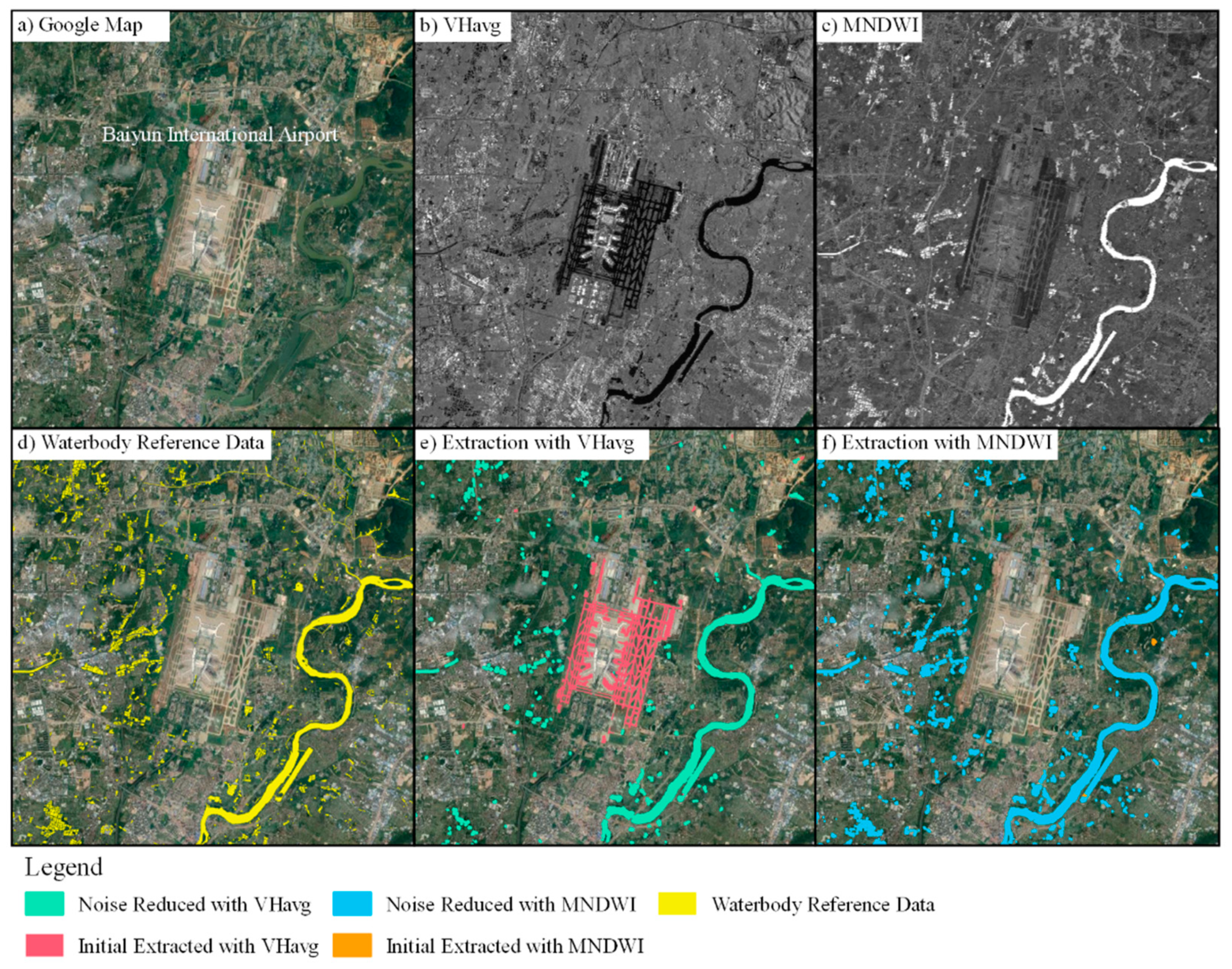
Figure 7 shows a typical case where the runway of Guangzhou Baiyun International Airport was misidentified as a waterbody using VHavg in initially extracted results and was then removed using flat surface removal by NDBI. There were similar noises, including viaducts, highways, playgrounds, and golf courses, that occurred in the results of VHavg. However, they did not appear in the results of MNDWI.
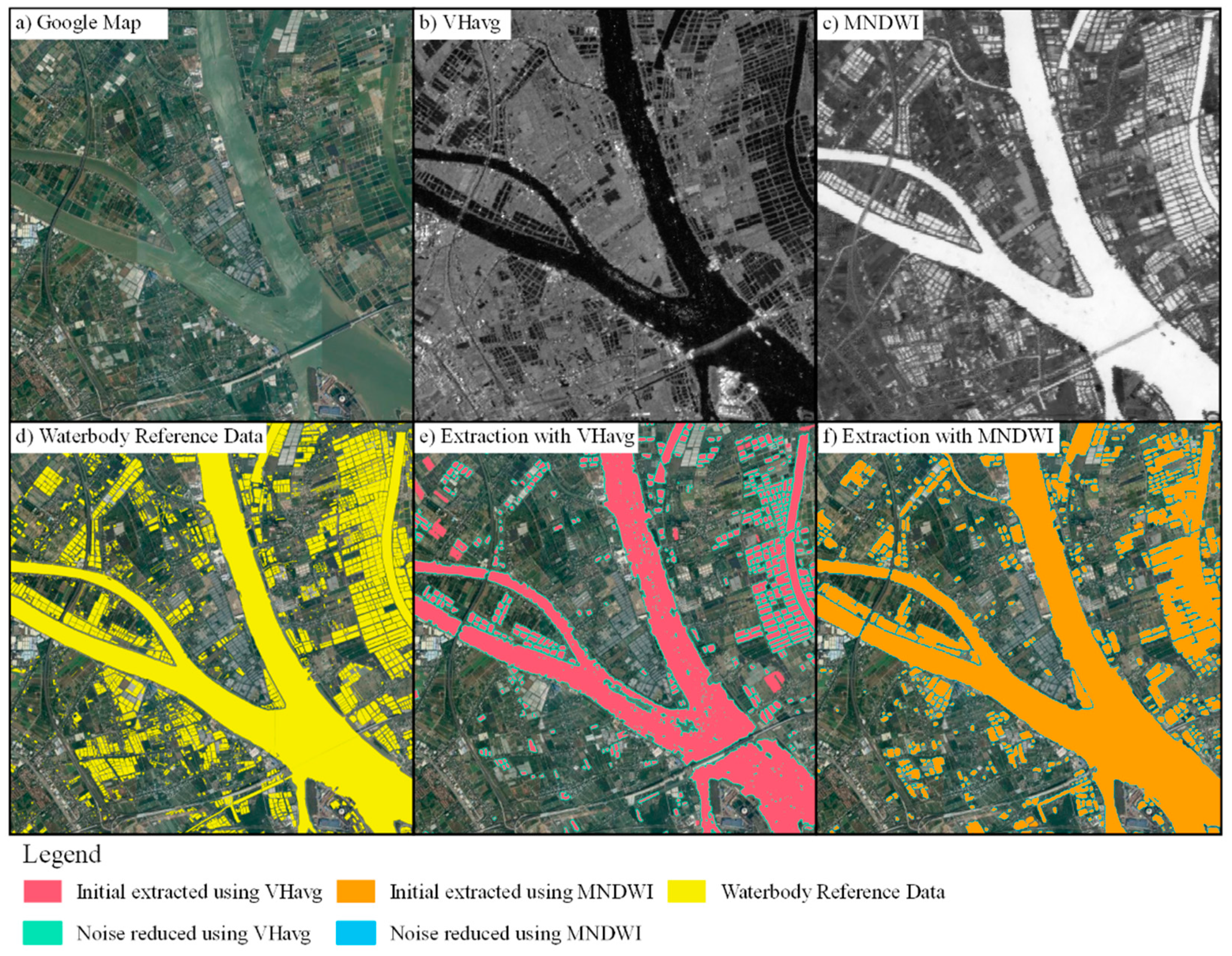
Typically, the composition of time series backscatter coefficients such as averaging can help reduce random factors such as speckle noise or sidelobes. However, for some waterways with intensive ship traffic, such as those shown in Figure 8, the value of the average backscatter coefficients was high, making the rivers extracted by VHavg reasonably fragmented.
4.2. Comparison of Sentinel-1A & 2 in Waterbody Mapping
To enable comparing the two datasets, VHavg and MNDWI, we used the same training data and training methods to determine the parameters in the waterbody mapping framework. As Table 2, Table 3 and Table 4 show, the MNDWI outperformed the VHavg in most of the metrics overall, especially F-measurea and F-measuren, with an increase of 9 and 16 percentage points, respectively.
We also found that the MNDWI was more likely to cause commission errors through the inspection results, while VHavg was more likely to cause omission errors. For a large number of small ponds, shown in Figure 9, the VHavg identified them as small pond individuals but missed many, while MNDWI identified them as a whole.
4.3. The Smallest Identifiable Area of Waterbody
Sentinel-1 and Sentinel-2 were proved to be high-quality data sources for monitoring the water surface. In our case, the two datasets, VHavg and MNDWI, exhibited similar performance in small waterbodies (smaller than 103 m2) and large waterbodies (larger than 106 m2). Both datasets were nearly incapable of identifying small waterbodies. However, the MNDWI outperformed the VHavg in medium waterbodies (larger than 103 m2 but smaller than 106 m2) identification. Especially for MNDWI, the SIWAL was larger than 104 m2; for VHavg, the SIWAL was larger than 107 m2.
5. Conclusions
In this paper, we evaluated the performance of two datasets, Sentinel-1A and Sentinel-2, on the mapping of small waterbodies over urban and mountainous regions. First, we applied an existing two-stage framework of waterbody mapping using two datasets. Notably, we used the same training data and training methods to determine the parameters of the framework. Then, we performed the validation by comparing the extracted waterbody results with 1-m spatial resolution reference waterbody data, which was delineated from Google Maps over Guangzhou, China. The assessment metrics of Precision, Recall, and F-measure were employed. The results showed that: (1) The MNDWI outperformed the VHavg by 9 percentage points of the F-measure. (2) There was more room for the results of VHavg to improve the accuracy in combination with noise reduction, i.e., the Precision of noise reduction could be improved by 4 percentage points with 1 percentage point cost in Recall. (3) The potential smallest identifiable waterbody area (Recall rate larger than 0.8) was larger than 104 m2. Future work will evaluate the waterbody mapping methods using GF-2 data of 0.8 m (high-resolution) in Guangdong Province, China.
Author Contributions
H.J. proposed and implemented the method, designed the experiments, and drafted the manuscript. M.W. contributed to the improvement of the proposed method and helped in the experimental design. H.H. and J.X. contributed to the improvement of the proposed method. All authors have read and agreed to the published version of the manuscript.
Funding
This work was jointly supported by the Open Research Fund Program of Key Laboratory of Agricultural Big Data, Ministry of Agriculture and Rural Affairs; Guangdong Province Agricultural Science and Technology Innovation and Promotion Project under grant number 2020KJ102; GDAS’ Project of Science and Technology Development under grant number 2020GDASYL-20200103004; Natural Science Foundation of Guangdong Province under grant number 2020A1515010643; Guangzhou Basic Research Project under grant number 202002020076; China Central Public-Interest Scientific Institution Basal Research Fund under grant number Y2020PT14; and Basal Research Fund of AII CAAS under grant number JBYW-AII-2020-17.
Institutional Review Board Statement
Not applicable.
Informed Consent Statement
Not applicable.
Data Availability Statement
The data presented in this study with resolution of equal to or above 10 m are available on request from the first author.
Conflicts of Interest
The authors declare that they do not have any conflict of interest.
References
- Pekel, J.-F.; Cottam, A.; Gorelick, N.; Belward, A.S. High-resolution mapping of global surface water and its long-term changes. Nature 2016, 540, 418–422. [Google Scholar] [CrossRef] [PubMed]
- Lehner, B.; Döll, P. Development and validation of a global database of lakes, reservoirs and wetlands. J. Hydrol. 2004, 296, 1–22. [Google Scholar] [CrossRef]
- Ding, X.; Nunziata, F.; Li, X.; Migliaccio, M. Performance Analysis and Validation of Waterline Extraction Approaches Using Single- and Dual-Polarimetric SAR Data. IEEE J. Sel. Top. Appl. Earth Obs. Remote Sens. 2017, 8, 1019–1027. [Google Scholar] [CrossRef]
- Jiang, H.; Feng, M.; Zhu, Y.; Lu, N.; Huang, J.; Xiao, T. An Automated Method for Extracting Rivers and Lakes from Landsat Imagery. Remote Sens. 2014, 6, 5067–5089. [Google Scholar] [CrossRef] [Green Version]
- Xiucheng, Y.; Shanshan, Z.; Xuebin, Q.; Na, Z.; Ligang, L. Mapping of Urban Surface Water Bodies from Sentinel-2 MSI Imagery at 10 m Resolution via NDWI-Based Image Sharpening. Remote Sens. 2017, 9, 596. [Google Scholar]
- Zhang, G.; Zheng, G.; Gao, Y.; Xiang, Y.; Lei, Y.; Li, J. Automated Water Classification in the Tibetan Plateau Using Chinese GF-1 WFV Data. Photogramm. Eng. Remote Sens. 2017, 83, 33–43. [Google Scholar] [CrossRef]
- Zhang, Z.; He, H.; Yu, C.; Zhang, W.; Li, L. Using the modified two-mode method to identify surface water in Gaofen-1 images. J. Appl. Remote Sens. 2018, 13, 1. [Google Scholar] [CrossRef]
- Hanqiu, X.U. Modification of normalised difference water index (NDWI) to enhance open water features in remotely sensed imagery. Int. J. Remote Sens. 2006, 27, 3025–3033. [Google Scholar]
- McFeeters, S.K. The use of the Normalized Difference Water Index (NDWI) in the delineation of open water features. Int. J. Remote Sens. 1996, 17, 1425–1432. [Google Scholar] [CrossRef]
- Kuenzer, C.; Guo, H.; Huth, J.; Leinenkugel, P.; Li, X.; Dech, S. Flood Mapping and Flood Dynamics of the Mekong Delta: ENVISAT-ASAR-WSM Based Time Series Analyses. Remote Sens. 2013, 5, 687–715. [Google Scholar] [CrossRef] [Green Version]
- Tanguy, M.; Chokmani, K.; Bernier, M.; Poulin, J.; Raymond, S. River flood mapping in urban areas combining Radarsat-2 data and flood return period data. Remote Sens. Environ. 2017, 198, 442–459. [Google Scholar] [CrossRef] [Green Version]
- Bioresita, F.; Puissant, A.; Stumpf, A.; Malet, J. A Method for Automatic and Rapid Mapping of Water Surfaces from Sentinel-1 Imagery. Remote Sens. 2018, 10, 217. [Google Scholar] [CrossRef] [Green Version]
- Huang, C.; Nguyen, B.D.; Zhang, S.; Cao, S.; Wagner, W. A Comparison of Terrain Indices toward Their Ability in Assisting Surface Water Mapping from Sentinel-1 Data. ISPRS Int. J. Geo-Inf. 2017, 6, 140. [Google Scholar] [CrossRef] [Green Version]
- Lu, D.; Weng, Q. A survey of image classification methods and techniques for improving classification performance. Int. J. Remote Sens. 2007, 28, 823–870. [Google Scholar] [CrossRef]
- Frazier, P.S.; Page, K.J. Water Body Detection and Delineation with Landsat TM Data. Photogramm. Eng. Remote Sens. 2000, 66, 1461–1467. [Google Scholar]
- Bonafilia, D.; Tellman, B.; Anderson, T.; Issenberg, E. Sen1Floods11: A Georeferenced Dataset to Train and Test Deep Learning Flood Algorithms for Sentinel-1. In Proceedings of the IEEE/CVF Conference on Computer Vision and Pattern Recognition (CVPR) Workshops, Seattle, WA, USA, 14–19 June 2020; pp. 835–845. [Google Scholar] [CrossRef]
- Yang, X.; Qin, Q.; Grussenmeyer, P.; Koehl, M. Urban surface water body detection with suppressed built-up noise based on water indices from Sentinel-2 MSI imagery. Remote Sens. Environ. 2018, 219, 259–270. [Google Scholar] [CrossRef]
- Zhe, Z.; Shixiong, W.; Woodcock, C.E. Improvement and expansion of the Fmask algorithm: Cloud, cloud shadow, and snow detection for Landsats 4–7, 8, and Sentinel 2 images. Remote Sens. Environ. 2015, 159, 269–277. [Google Scholar] [CrossRef]
- Introduction of Guangdong Province. Available online: http://www.gd.gov.cn/zjgd/sqgk/zrdl/index.html (accessed on 25 March 2021).
- Topography of Guangzhou City. Available online: http://nyncj.gz.gov.cn/sj/sn/dxdm/ (accessed on 24 November 2020).
- Guangzhou Water Resources Bulletin. 2018. Available online: http://swj.gz.gov.cn/attachment/0/45/45140/5298825.pdf (accessed on 24 November 2020).
- Sentinel-1 SAR User Guide. Available online: https://sentinel.esa.int/web/sentinel/user-guides/sentinel-1-sar (accessed on 25 March 2021).
- Sentinel-2 User Handbook. Available online: https://sentinel.esa.int/documents/247904/685211/Sentinel-2_User_Handbook (accessed on 25 March 2021).
- Ubukawa, T. An Evaluation of the Horizontal Positional Accuracy of Google and Bing Satellite Imagery and Three Roads Data Sets Based on High Resolution Satellite Imagery; Center for International Earth Science Information Network (CIESIN) The Earth Institute at Columbia University: New York, NY, USA, 2013. [Google Scholar]
- Zhang, Z.; Zhang, X.; Jiang, X.; Xin, Q.; Ao, Z.; Zuo, Q.; Chen, L. Automated Surface Water Extraction Combining Sentinel-2 Imagery and OpenStreetMap Using Presence and Background Learning (PBL) Algorithm. Sel. Top. Appl. Earth Obs. Remote Sens. IEEE J. 2019, 12, 3784–3798. [Google Scholar] [CrossRef]
- Cai, L.; Shi, W.; Miao, Z.; Hao, M. Accuracy Assessment Measures for Object Extraction from Remote Sensing Images. Remote Sens. 2018, 10, 303. [Google Scholar] [CrossRef] [Green Version]
Figure 1.
The study area of Guangzhou, China.

Figure 2.
Waterbody reference data (WRD) of Guangzhou City.

Figure 3.
The framework of waterbody mapping using either Sentinel-1A SAR or Sentinel-2 optical input data.
Figure 3.
The framework of waterbody mapping using either Sentinel-1A SAR or Sentinel-2 optical input data.

Figure 4.
The VHavg backscatter coefficient distributions for non-water and waterbodies at different area sizes. Note that the VH backscatter coefficient value of each waterbody is the median of pixel values associated with each waterbody.
Figure 4.
The VHavg backscatter coefficient distributions for non-water and waterbodies at different area sizes. Note that the VH backscatter coefficient value of each waterbody is the median of pixel values associated with each waterbody.

Figure 5.
The MNDWI (Modified Normalized Difference Water Index) distributions for non-water and waterbodies of different area sizes. Note the MNDWI value of each waterbody is the median of pixel value associated with each waterbody.
Figure 5.
The MNDWI (Modified Normalized Difference Water Index) distributions for non-water and waterbodies of different area sizes. Note the MNDWI value of each waterbody is the median of pixel value associated with each waterbody.

Figure 6.
Waterbody identification results: a case of noise reduction for mountain shadows.

Figure 7.
Waterbody identification results: a case of noise reduction for flat surfaces.

Figure 8.
Waterbody identification results: a case of noise reduction for holes caused by ships in waterways.
Figure 8.
Waterbody identification results: a case of noise reduction for holes caused by ships in waterways.

Figure 9.
Waterbody identification results: a case of pond identification.


Table 1.
Statistics of waterbody reference data.
| Waterbody Type | Description | Number of Polygons | Total Area (km2) |
|---|---|---|---|
| Rivers | The main stream and tributaries of the Pearl River | 652 | 335.23 |
| Channels | Drainage channels in urban areas or ditches for drainage and irrigation in rural areas. | 221 | 1.85 |
| Reservoirs | Mainly distributed in northern Guangzhou | 255 | 38.70 |
| Lakes | Lakes for tourism in urban areas | 28 | 1.46 |
| Ponds | Mainly ponds for aquaculture | 74,212 | 279.39 |
Table 2.
Accuracy of identification of waterbody area.
| Method | Dataset | Precisiona | Recalla | F-Measurea |
|---|---|---|---|---|
| Initial extracted | VHavg | 0.835 | 0.547 | 0.661 |
| MNDWI | 0.818 | 0.705 | 0.757 | |
| Noise reduced | VHavg | 0.878 | 0.532 | 0.662 |
| MNDWI | 0. 824 | 0.692 | 0.752 |
Table 3.
Accuracy of identification of waterbody number.
| Method | Dataset | Precisionn | Recalln | F-Measuren |
|---|---|---|---|---|
| Initial extracted | VHavg | 0.703 | 0.151 | 0.249 |
| MNDWI | 0.853 | 0.269 | 0.409 | |
| Noise reduced | VHavg | 0.707 | 0.144 | 0.239 |
| MNDWI | 0.842 | 0.262 | 0.400 |
Table 4.
Recalln rate of identified waterbodies of different area levels.
| Waterbody Area (m2) | Waterbody Number | Recalln | |
|---|---|---|---|
| VHavg | MNDWI | ||
| 102 | 340 | 0 | 0.009 |
| 103 | 15015 | 0.005 | 0.028 |
| 104 | 22854 | 0.167 | 0.334 |
| 105 | 3235 | 0.621 | 0.847 |
| 106 | 109 | 0.661 | 0.770 |
| 107 | 20 | 0.750 | 0.800 |
| 108 | 4 | 1.000 | 1.000 |
Publisher’s Note: MDPI stays neutral with regard to jurisdictional claims in published maps and institutional affiliations. |
© 2021 by the authors. Licensee MDPI, Basel, Switzerland. This article is an open access article distributed under the terms and conditions of the Creative Commons Attribution (CC BY) license (https://creativecommons.org/licenses/by/4.0/).
Share and Cite
MDPI and ACS Style
Jiang, H.; Wang, M.; Hu, H.; Xu, J. Evaluating the Performance of Sentinel-1A and Sentinel-2 in Small Waterbody Mapping over Urban and Mountainous Regions. Water 2021, 13, 945. https://doi.org/10.3390/w13070945
AMA Style
Jiang H, Wang M, Hu H, Xu J. Evaluating the Performance of Sentinel-1A and Sentinel-2 in Small Waterbody Mapping over Urban and Mountainous Regions. Water. 2021; 13(7):945. https://doi.org/10.3390/w13070945
Chicago/Turabian StyleJiang, Hao, Mo Wang, Hongda Hu, and Jianhui Xu. 2021. "Evaluating the Performance of Sentinel-1A and Sentinel-2 in Small Waterbody Mapping over Urban and Mountainous Regions" Water 13, no. 7: 945. https://doi.org/10.3390/w13070945
Note that from the first issue of 2016, this journal uses article numbers instead of page numbers. See further details here.