
Quantifying the Impact of Evapotranspiration at the Aquifer Scale via Groundwater Modelling and MODIS Data


1
SIMAU—Department of Materials, Environmental Sciences and Urban Planning, Polytechnic University of Marche, 60131 Ancona, Italy
2
DiSTABiF—Department of Environmental, Biological and Pharmaceutical Sciences and Technologies, Campania University “Luigi Vanvitelli”, 81100 Caserta, Italy
3
DICEA—Department of Civil and Building Engineering and Architecture, Polytechnic University of Marche, 60131 Ancona, Italy
*
Author to whom correspondence should be addressed.
Water 2021, 13(7), 950; https://doi.org/10.3390/w13070950
Submission received: 19 February 2021
/
Revised: 28 March 2021
/
Accepted: 30 March 2021
/
Published: 31 March 2021
(This article belongs to the Special Issue Evapotranspiration Measurements and Modeling)
Abstract
:In shallow alluvial aquifers characterized by coarse sediments, the evapotranspiration rates from groundwater are often not accounted for due to their low capillarity. Nevertheless, this assumption can lead to errors in the hydrogeological balance estimation. To quantify such impacts, a numerical flow model using MODFLOW was set up for the Tronto river alluvial aquifer (Italy). Different estimates of evapotranspiration rates were retrieved from the online Moderate Resolution Imaging Spectroradiometer (MODIS) database and used as input values. The numerical model was calibrated against piezometric heads collected in two snapshots (mid-January 2007 and mid-June 2007) in monitoring wells distributed along the whole alluvial aquifer. The model performance was excellent, with all the statistical parameters indicating very good agreement between calculated and observed heads. The model validation was performed using baseflow data of the Tronto river compared with the calculated aquifer–river exchanges in both of the simulated periods. Then, a series of numerical scenarios indicated that, although the model performance did not vary appreciably regardless of whether it included evapotranspiration from groundwater, the aquifer–river exchanges were influenced significantly. This study showed that evapotranspiration from shallow groundwater accounts for up to 21% of the hydrogeological balance at the aquifer scale and that baseflow observations are pivotal in quantifying the evapotranspiration impact.
1. Introduction
Evapotranspiration exerts a key role in watershed water budgets [1] and a wide range of techniques have been developed to accurately characterize its spatial and temporal variability at site specific locations, mainly using surface energy balance methods [2,3] and surface water balance methods [4,5]. Evapotranspiration is generally considered in surface water hydrological modelling [6] by spatially integrating semi-empirical formulas based on climate variables, such as temperature, humidity, wind speed, and solar radiation, included in the Penman–Monteith [7] or Priestley–Taylor [8] formulas and their global assessment [9].
Despite the key importance of evapotranspiration in surface water hydrological modeling, the latter is not often directly included in groundwater flow models at the aquifer scale [10,11]. This is due to the fact that direct evapotranspiration from groundwater is generally considered to be negligible in aquifers, especially if they are formed by coarse grained sediments, which are characterized by low capillary rise [12]. For this reason, evapotranspiration is often subtracted from precipitation to gain recharge estimates used as an input in groundwater flow models [13], especially when the water table is relatively deep [14]. Moreover, an accurate estimation of evapotranspiration, especially in heterogeneous landscapes, can be difficult to obtain due to many driving factors, which can make extrapolation of data inaccurate, and thus mean evapotranspiration values are often used for the whole modeled domain [15,16]. To overcome these simplifications, a growing legacy of remote sensing techniques has appeared in the literature during the past decade [17,18,19], with the aim to better quantify the spatial and temporal estimates of evapotranspiration rates at the aquifer scale. Direct assimilation of remote sensing data into land surface models is a topical research subject [20,21,22,23], but there is still not enough information on evapotranspiration estimates via remote sensing techniques in groundwater models.
Few and sparse regional groundwater flow models have included remote sensing data in their workflow [24,25] due to the inherent difficulties in retrieving consistent observed data at the whole aquifer scale. Few well-documented cases have been developed to date at the scales comparable to those of this study [26,27], but there is still a lack of detailed groundwater flow models exploring the impact of evapotranspiration on the hydrogeological water budget in different climates. Recently, the Moderate Resolution Imaging Spectroradiometer (MODIS) evapotranspiration products have proven to be reliable and highly useful tools, because they are free downloadable datasets and consequently relatively easy to use by researchers and governments stakeholders [28]. They have been successfully used for multi-calibration purposes in several surface models [29,30], providing crucial information, particularly in ungauged basins. Thus, to overcome the lack of evapotranspiration factors in groundwater flow modeling, this study aimed (i) to quantify the role of direct evapotranspiration from shallow groundwater incorporating remote sensing data in an aquifer-scale groundwater model; and (ii) to assess the model sensitivity to evapotranspiration rate estimations via remote sensing techniques.
2. Materials and Methods
2.1. Hydrogeological Setting
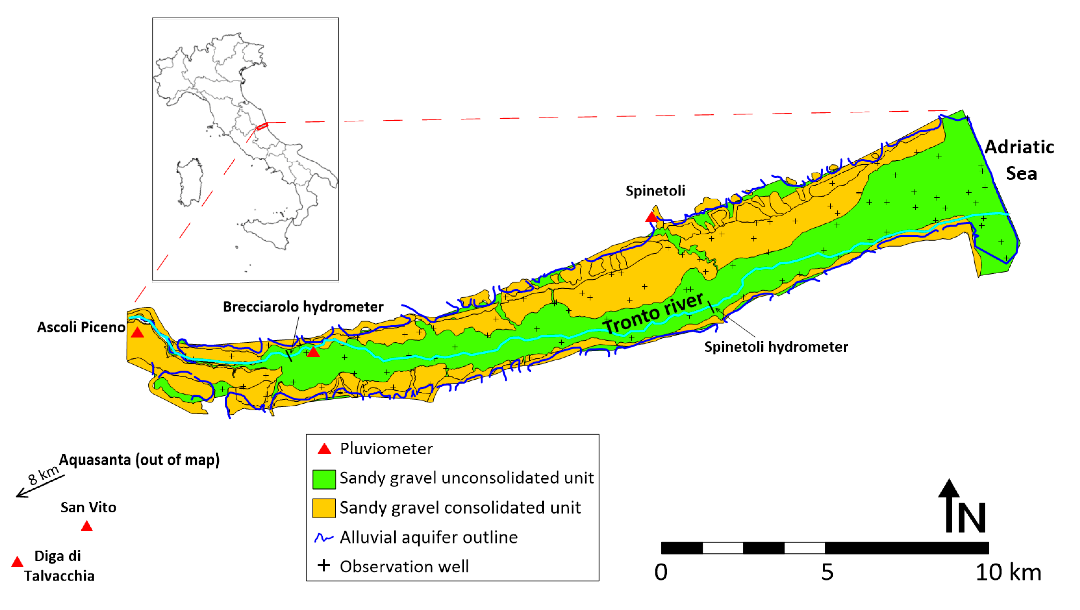
The drainage basin of the Tronto river, one of the major rivers of the Adriatic side of Central Italy, extends over 1192 km2 between Abruzzo and Marche regions, and is stretches WSW–ENE. Its alluvial aquifer covers an extension of 56.4 km2 from Ascoli-Piceno town (140 m asl) to the Adriatic Sea. The river is 115 km long, and has a mean gradient of 2.1% and a 32 km long alluvial plain, oriented E–W with a mean gradient of 0.4%. The alluvial plain has been subdivided into three sectors: piedmont, mid-valley and coastal [31]. The piedmont sector, about 6 km long, is characterized by a relatively steep longitudinal profile and a narrow thalweg delimited by a high and vertical scarp that creates a small gorge. In the mid-valley sector, which is 21 km long, the thalweg enlarges progressively and is bordered by a large alluvial plain; it has a gentler longitudinal profile and confined terraces. The coastal sector, about 4 km long, is characterized by a still smaller gradient, a greater width of the valley, and an elongated sandy coastline [31]. The climate in the Tronto watershed is of the “central-southern Adriatic” type in the lower valley and “Apennine” in the mountainous part. As with most Mediterranean regions, it has mild winters and hot dry summers [32]. The maximum peak discharge of the Tronto river is 1320 m3/s, and the mean discharge and baseflow are 17.8 and 2.5 m3/s, respectively [31].
The unconfined alluvial aquifer is composed of two hydrogeological units [33]: (i) the highly permeable sandy gravel unit located in the recent unconsolidated alluvial deposits and (ii) the partially cemented sandy gravel unit located in the older terraces outcropping at both flacks of the Tronto valley but mainly developed in the Northern flank (Figure 1).
The bedrock is made of Plio-Pleistocene consolidated clays that behave as aquiclude [33]. The typical stratigraphy is characterized by medium to fine planar and trough cross-bedded gravels with local layers of horizontally bedded gravels [31]. A total number of 143 stratigraphic logs were used to recognize the subsurface lithologies and the bedrock location.
In January 2007 (from 15th to 19th) and June 2007 (from 15th to 19th), two groundwater level monitoring campaigns were performed in observation wells (Figure 1) scattered through the alluvial aquifer. The number of observation wells were 84 for January 2007 and 70 for June 2007. The average hydraulic conductivity of the two hydrogeological units was determined from 22 slug tests in monitoring wells and 7 pumping tests; the unconsolidated sandy gravel unit had an average value of 3.1 × 10⁻³ m/s, and the consolidated sandy gravel unit had an average value of 2.4 × 10⁻⁴ m/s.
2.2. Groundwater Flow Model Set Up
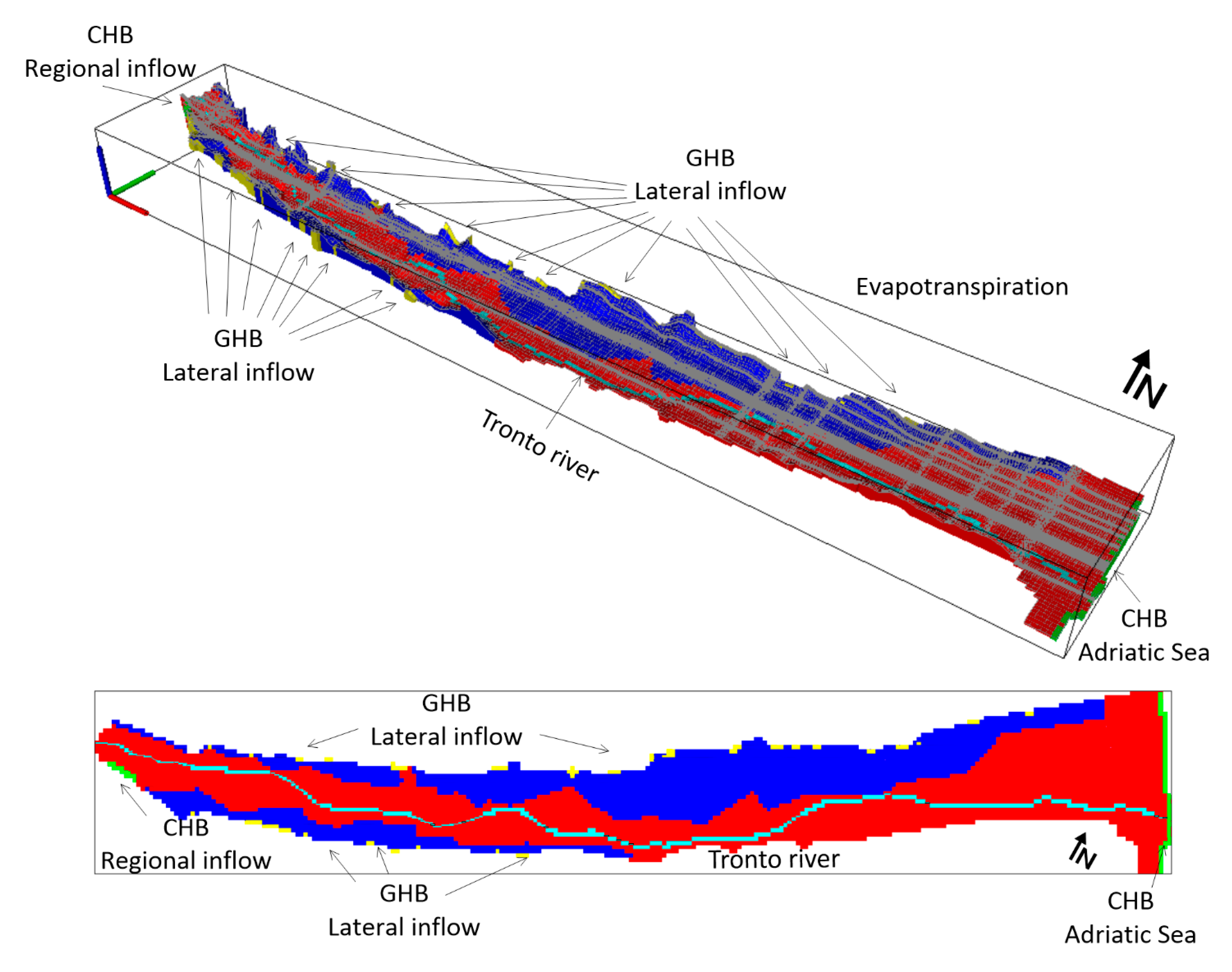
By using all the available hydrogeological and stratigraphic information, a three-dimensional, groundwater flow model was established. The United States Geological Service (USGS) flow model MODFLOW-2005 [34] was used, and pre- and post-processing was conducted using the graphical user interface Processing Modflow 8.0 [35]. Model-viewer 1.7 was used for three-dimensional post-processing [36]. MODFLOW-2005 is designed to simulate three-dimensional saturated groundwater flow in porous media. The active model domain was initially discretized into a regular spaced grid of 100 m × 100 m, then refined down 10 m × 10 m in those areas where pumping wells were located (Figure 2). Vertically the model domain was discretized into a single layer with variable thicknesses (mean thickness 18.0 m). The top of the grid was interpolated using a 10 m × 10 m digital terrain model, ranging from 1.1 m to 136.4 m asl. The bottom of the grid, representing the top of the underlying bedrock (Plio-Pleistocene consolidated clays unit), ranged from −37.1 to 120.7 m asl, and was interpolated using information from stratigraphic logs.
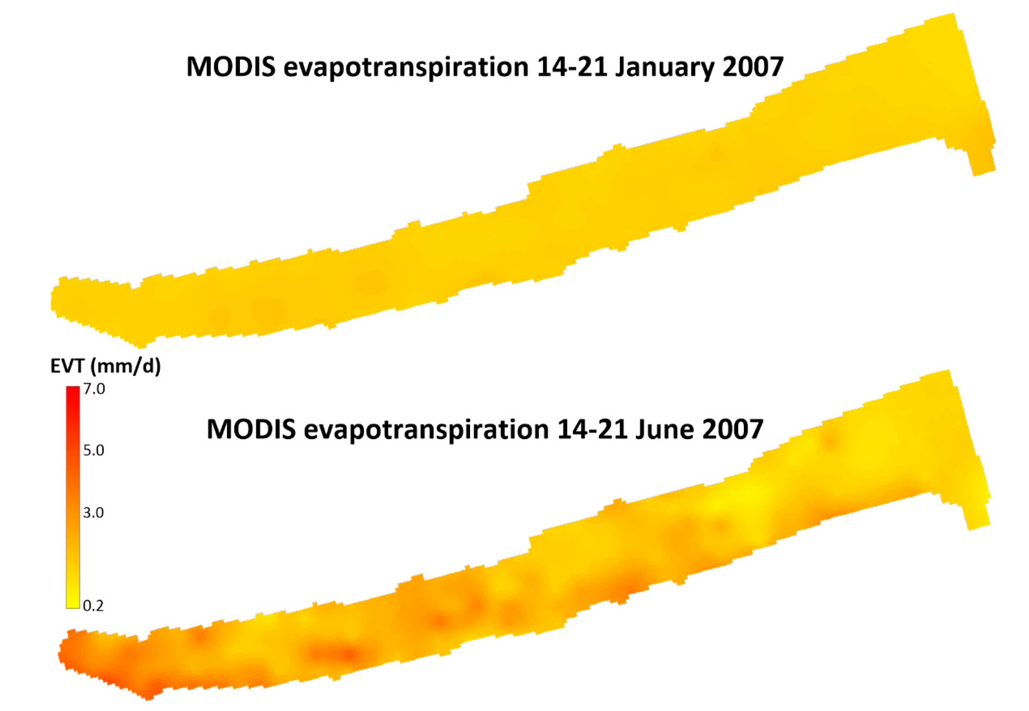
The CONSTANT HEAD BOUNDARY package (CHB) was used to represent the regional groundwater inflow boundary and the Adriatic Sea boundary. The inflow CHB was set using the hydrometric head of the Castellano stream (130 m asl in both January and June 2007 simulations), which is a major affluent of the Tronto river located near this boundary. The Castellano stream drains a fractured aquifer structure which provides a constant baseflow to the Castellano stream [37]. The RIVER package (RIV) was employed to simulate the Tronto river; the GENERAL HEAD BOUNDARY package (GHB) was used to represent the lateral groundwater flow from ephemeral Tronto effluents; and the WELL package (WEL) was used to simulate the pumping rate of the principal wells present in the alluvial aquifer with a known pumping rate. The information on pumping wells was collected from the Regional Basin Authority, which created a land registry with location, depth, and radius of each well, and declared pumping rate; here, only pumping wells with a continuous pumping rate of more than 5.0 L/s were included in the model (16 wells). The EVAPOTRANSPIRATION package (EVT) was used to simulate the evapotranspiration from groundwater, with the evapotranspiration rate derived from the Moderate Resolution Imaging Spectroradiometer (MODIS) dataset. The algorithm used for the MOD16 data product collection is based on the logic of the Penman–Monteith equation [38], which includes inputs of daily meteorological reanalysis data and MODIS remotely sensed data products, such as vegetation property dynamics, albedo, and land cover [39]. The MOD16A2 Version 6 Total Evapotranspiration product is an 8-day composite dataset produced at 500 m pixel resolution. The data were download from the MOD16A2GF model [38] using the AppEARS interface [40] and further converted into point features to allow a proper spatial distribution of the study area through the application of kriging interpolation [41] over the model grid. (Figure 3). The extinction depth of evapotranspiration for June 2007 was set to 1.5 m below ground level because this is the suggested value for cropped fields in permeable soils [12]. For January 2007, extinction depth was set to 0.9 m below ground level because only evaporation played a role given that in wintertime the soils are generally uncropped, and the transpiration of plants is basal [42].
2.3. Baseflow Monitoring Strategy
To obtain the hydrological data on the investigated basin, a network of rain-gauge stations and two hydrometric stations belonging to the Civil Protection Agency of Marche Regional Authority was analyzed (Figure 1).
Six rain-gauge stations were positioned at different elevations throughout the Tronto alluvial aquifer and on the nearby mountain area, with elevations ranging from 52 to 688 m asl (Table 1). During the weeks when the piezometric campaigns were performed (from 14 to 20 January and June 2007) no precipitations were recorded in all stations except for the 18th of January, when a modest event occurred within the watershed, especially at mountainous locations and higher elevations (e.g., Amatrice and Arquata del Tronto, with elevations of 922 and 700 m asl, respectively). This event slightly affected the global watershed balance, which is ruled by the classical law:
where the precipitation (P) is balanced by the runoff/basin discharge (Q), evapotranspiration (EVT), and storage variation (ΔS). However, due to the small precipitation within the study area, i.e., between Ascoli Piceno and Spinetoli (see Figure 1), no major differences existed at either location in terms of runoff and recharge contributions during the monitoring period. Two hydrometric stations of the Tronto river with rating curves were available, the first positioned near to the alluvial aquifer upstream boundary (Brecciarolo), and a second (Spinetoli) in the mid-valley sector. Their flow rates were analyzed to obtain the exchange fluxes between the alluvial aquifer and the Tronto river during baseflow recession periods. A third hydrometric station was operating during the analyzed period along the Tronto river, but this could not be used for the present analysis due to the strong tidal influence that is typically observed in microtidal environments, even some kilometers far from the river mouth [43].
P = Q + EVT + ΔS
The average daily flow rates of the upstream and downstream sections were used to estimate the flow rate variation along the selected Tronto river branch. The obtained flow rates were further processed using the Base Flow Index (BFI) software [44], a simple approach which separates surface runoff and baseflow [45], to determine the baseflow component between the two gauging stations in mid-January and mid-June 2007. The observed baseflow rates were then compared with the calculated baseflow rates using the WATERBUDGET subroutine of MODFLOW-2005, which allows subregions to be defined for which a water budget is to be calculated, in this case, the portion of the model domain between Brecciarolo and Spinetoli gauging stations (Figure 1).
2.4. Model Calibration, Validation and Scenarios
All of the simulations were run in steady-state mode, after an initial trial and error calibration procedure. An automated calibration was performed via the inverse code PEST [46], combined with an automated sensitivity analysis. The automated calibration was done on: (i) horizontal hydraulic conductivity of the two hydrogeological units, (ii) conductance of riverbed, and (iii) conductance of GHB. PEST handles the employment of prior information on parameters to stabilize the search of optimal values into physically based estimates and to minimize computational time. The objective function on which PEST performed the calibration consisted of all of the available head observations in each monitored period. The Nash–Sutcliffe model efficiency coefficient (NSE), the percentage of bias (PB), and the absolute mean error (AME) were used to evaluate model performance. The model estimates were validated comparing observed fluxes among the Tronto river and the aquifer in the two monitored periods, as explained in the previous section. Once the model was considered calibrated and validated, a series of scenarios were examined to quantify the impact of evapotranspiration on the groundwater budget. First, to analyze the role of the spatialization of the evapotranspiration versus mean values at the aquifer scale, the average monthly evapotranspiration rates were retrieved from the MODIS database for both January (1.62 mm/d) and June 2007 (7.68 mm/d). These values were used as mean evapotranspiration rate values applied to the whole aquifer in two simplified scenarios, named EVT-Mean-01/07 and EVT-Mean-06/07, respectively. In addition, two other simplified scenarios using the 8-day average evapotranspiration rates extracted from the data shown in Figure 3 were constructed and named EVT-Mean-14–21/01/07 (2.31 mm/d) and EVT-Mean-14–21/06/07 (4.75 mm/d), respectively. Finally, two basic scenarios were run by disabling the EVT package to quantify the impact of evapotranspiration from shallow groundwater at the aquifer scale. The latter scenarios were named NO-EVT-01/07 and NO-EVT-06/07, respectively. A sensitivity analysis was also performed on the calibrated model using single perturbation tests (±10% of the employed parameter values) on both evapotranspiration rates and extinction depths, because the PEST automated sensitivity analysis included in Processing Modflow 8.0 cannot handle the extinction depth as parameter.
3. Results and Discussion
3.1. Groundwater Flow Model Results
The initial estimates of hydraulic conductivity for the two hydrogeological units were only slightly changed during the model calibration process (Table 2). The river conductance decreased from January to June 2007, which could be due to changes in river morphology or hydraulic conductivity of the riverbed. The latter cannot be considered constant over time due to depositional and erosional patterns of flooding events, which can abruptly alter this parameter. The GHB conductance also changed between the two simulated periods, significantly increasing in June 2007 with respect to January 2007. This was due to the small lateral creeks’ reactivation during the spring season that sustained the baseflow of the Tronto river in June 2007 (see following section). The highest composite sensitivity was found for the consolidated sandy gravel unit, followed by the sandy gravel unit and GHB conductance, whereas the Tronto river conductance only slightly affected the model composite sensitivity in both of the simulated periods (Table 2).
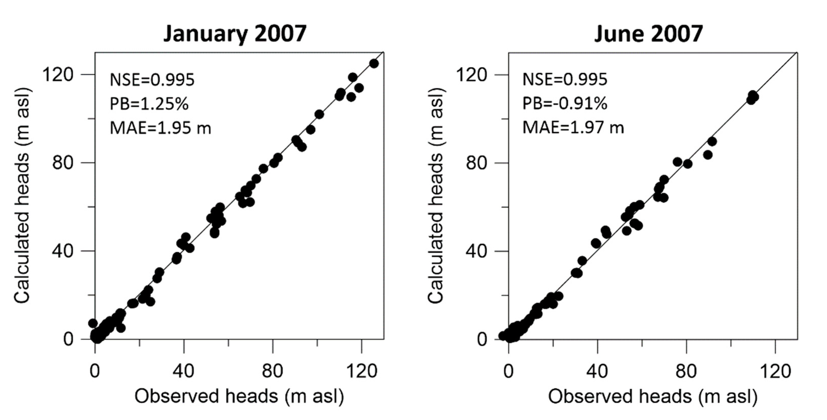
Figure 4 shows the calibration results of measured versus computed hydraulic heads in all of the monitoring wells (see Figure 1 for location). A very good model performance was achieved for both of the simulated periods. It must be stressed that the AME in both simulation periods was around 2 m, which is an acceptable, but non-negligible value considering the large variation of groundwater heads throughout the model domain (>120 m). This could be due to the steady state approach employed here, whereas the stream–aquifer system is transient by nature [47,48].
The calculated contour maps of the groundwater heads are displayed in Figure 5. Here the contribution of the regional groundwater flow in the upper part of the alluvial aquifer is evident, with the equipotential head contours converging towards the Tronto river in the piedmont sector and in the mid-valley. On the contrary, the coastal sector is characterized by lower head gradients and by slightly diverging equipotential head contours from the Tronto river. This behavior suggests that the Tronto river is gaining water from the aquifer in the upper sectors of the alluvial valley and losing water near the coast, as typically observed in many other Apennine rivers [33,49].
Moreover, the lateral creeks’ contribution to the general groundwater flow pattern was important given that simulations without lateral groundwater flow (i.e., GHB) lowered the groundwater heads at both sides of the alluvial aquifer, which in turn decreased the model performance indicators. Although the NSE remained elevated for both of the simulated periods (0.981 and 0.976 for January and June 2007, respectively), the PB and AME decreased significantly by −1.94% and 2.92 m for January 2007 and by 6.61% and 4.00 m for June 2007.
The contribution of the lateral creeks is more evident on the water balance of the model domain (Table 3). Here it is apparent that GHB (lateral creeks’ contribution) represented approximately 30% of the whole hydrogeological budget. More importantly, the evapotranspiration for the 14–21 January 2007 period was approximately 15% of the whole hydrogeological budget. Considering that, in wintertime, the evaporation component prevails, this is a remarkable result, meaning that the evaporation from groundwater alone can be highly relevant for the hydrogeological balance even in temperate climates. In fact, the evapotranspiration for the 14–21 June 2007 period, when the transpirative component in Central Italy is near the apex [50], reached a value near to 21% of the whole hydrogeological budget. Overall, this is a clear indication that direct evapotranspiration from groundwater cannot be neglected in groundwater flow models even in coarse grain soils with low capillaries.
3.2. Baseflow Monitoring Results
The daily average discharge and precipitation from January to July 2007 is plotted in Figure 6 for both the Brecciarolo (in blue) and Spinetoli (in red) gauging stations. The surface runoff–baseflow separation line, obtained from the BFI-software application, is shown with lighter colors at both river cross-sections. In addition to the hydropeaking fluctuations induced by upstream-located hydropower plants [51], the maximum flow peak occurs in the first half of April, promoted by a significant and intense precipitation (more than 30 mm/day), as shown by the downward-pointing gray lines. Further relevant flow peaks are due to milder but persistent precipitations at the end of January and the beginning of March. It is worth noting that the baseflow contribution at the downstream location (light red) is larger than at the upstream section (light blue) most of the time, mainly in spring and summer (April and July), probably due to the important role of the tributaries feeding the Tronto river between the analyzed stations. Further, just after the April rainfall and compared to the upstream section, a greater groundwater recharge and reduced surface contribution occurred at the downstream section. Focusing on the weeks under analysis, small flow rates were recorded at both stations, with flow rates around 2–3 m3/s in January (lower left panel) and 3–5 m3/s in June (lower right panel).
The BFI-calculated baseflow shows that the aquifer is recharging the Tronto river most of the time, but the relationship is not constant because, from February to April and at the end of July 2007 the aquifer is fed by the Tronto river, probably because the groundwater level dropped below the hydrometric level of the Tronto river. The mean baseflow rate calculated for the 14–20 January 2007 period was 1.04 ± 0.04 m3/s and for the 14–20 June 2007 period was 1.36 ± 0.06 m3/s. The calculated baseflow rates matched well with the model-calculated outflows from the aquifer towards the Tronto river branch from Brecciarolo to Spinetoli. These were 1.12 m3/s for the January 2007 simulation and 1.45 m3/s for the June 2007 simulation. Both simulations slightly overestimated the baseflow rates calculated with BFI, although the flow rate estimation is usually affected by errors that produce uncertainties up to 40% at a 95% confidence interval [52]. Considering the factors mentioned above, the calibrated groundwater flow model via observed heads was validated by the baseflow observations, thus the hydrogeological water balance can be considered reliable. To gain some insights into the effects of EVT rates on model performance, a series of model scenarios and a single parameter sensitivity analysis are outlined in the following section.
3.3. Scenario Modelling and Sensitivity Analysis
The model performance indicators and the difference between observed baseflow via BFI and model-calculated baseflow for the different scenarios using distributed and mean evapotranspiration rates are summarized in Table 4. It is clear that the statistical indicators (NSE, PB, and AME) did not vary substantially using the distributed evapotranspiration from MODIS at an interval of 8 days or the average evapotranspiration value for the whole aquifer in that week or in that month. However, a non-negligible discrepancy among the observed (via BFI) and modelled baseflow rates appears in the EVT-MODIS-Monthly Mean. This highlights the importance of including baseflow observations during the model calibration and validation procedures, because with sole head observations (despite being well-distributed in the model domain) it would be impossible to determine if a monthly mean evapotranspiration rate could be sufficient to accurately simulate the groundwater flow and balance processes. As already pointed out by Doble and Crosbie [13], additional calibration requirements are needed to better resolve the evapotranspiration role at the basin scale. In particular, estimates of groundwater fluxes, such as baseflow to streams, are fundamental.
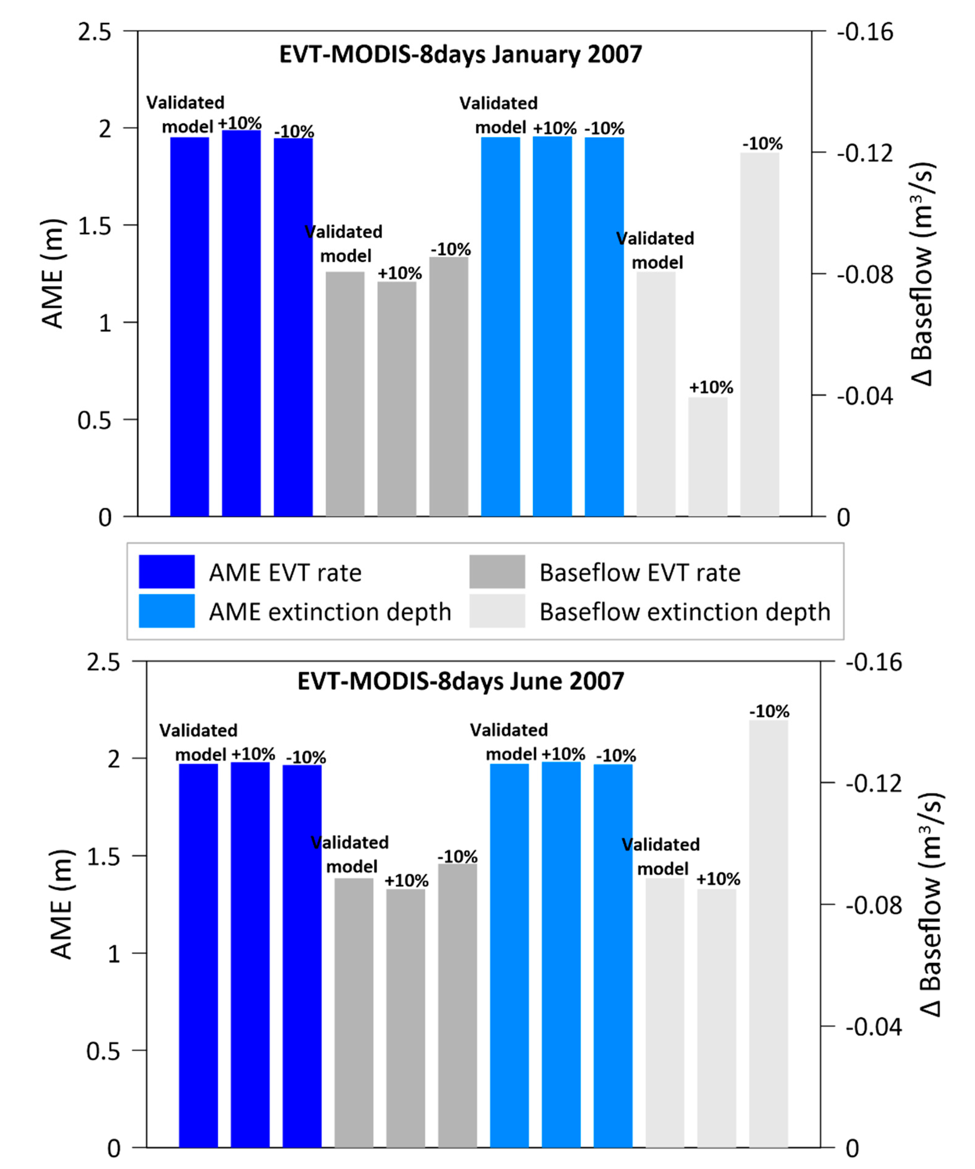
Finally, the single parameter sensitivity analysis was performed to elucidate the uncertainties on both evapotranspiration rate and extinction depth (Figure 7). The results highlighted a very weak sensitivity of both parameters to ±10% perturbations, with negligible differences on all the model performance indicators and with very small differences between observed and calculated baseflows; namely, the evapotranspiration rate perturbation induced a baseflow change of ±0.04 m3/s in January 2007 simulation and of ±0.02 m3/s in June 2007, and the extinction depth perturbation induced even lower changes (±0.004 m3/s in both simulations). This can be considered additional evidence that the numerical flow model was not largely sensitive to uncertainties in evapotranspiration rates and extinction depths.
Moreover, it has been recently observed that MODIS data are reliable compared to classical semi-empirical formulas to calculate a simplified water balance in karst aquifers in Southern Italy [53]. Thus, MODIS data could be used as evapotranspiration input data for regional scale numerical models to minimize the uncertainties on this key parameter.
4. Conclusions
This study quantified the role exerted by evapotranspiration from shallow groundwater at the aquifer scale, through direct assimilation of MODIS data as model input data. The validated model showed that evapotranspiration from groundwater accounted for up to 21% of the hydrogeological balance, thus it cannot be neglected. The use of averaged weekly values over the entire model domain did not substantially decrease the model performance indicators or the calculated baseflow, whereas using monthly averaged values resulted in larger discrepancies in the calculated baseflow but not in the model performance indicators based on groundwater heads. This highlights that baseflow observations are pivotal in quantifying the evapotranspiration impact at the aquifer scale. Based on stream–aquifer interactions through model coupling [54], future studies should focus on the transient behavior of the surface–groundwater interactions, with incorporation of weekly MODIS evapotranspiration rates over an entire hydrological year coupled with continuous baseflow observations. However, for such transient numerical models it is imperative to equip a network of monitoring wells with continuous groundwater level monitoring.
Author Contributions
Conceptualization, N.C.; methodology, N.C. and M.P.; software, N.C. and G.B.; validation, M.P.; formal analysis, N.C. and M.G.; investigation, M.G.; data curation, N.C.; writing—original draft preparation, N.C.; writing—review and editing, M.P., M.G. and G.B.; visualization, N.C. All authors have read and agreed to the published version of the manuscript.
Funding
This research received no external funding.
Institutional Review Board Statement
Not applicable.
Informed Consent Statement
Not applicable.
Data Availability Statement
Data are available from the corresponding author upon request.
Conflicts of Interest
The authors declare no conflict of interest.
References
- Wilson, K.B.; Hanson, P.J.; Mulholland, P.J.; Baldocchi, D.D.; Wullschleger, S.D. A comparison of methods for determining forest evapotranspiration and its components: Sap-flow, soil water budget, eddy covariance and catchment water balance. Agric. For. Meteorol. 2001, 106, 153–168. [Google Scholar] [CrossRef]
- Liou, Y.A.; Kar, S.K. Evapotranspiration estimation with remote sensing and various surface energy balance algorithms—A review. Energies 2014, 7, 2821–2849. [Google Scholar] [CrossRef] [Green Version]
- Bastiaanssen, W.G.M.; Cheema, M.J.M.; Immerzeel, W.W.; Miltenburg, I.J.; Pelgrum, H. Surface energy balance and actual evapotranspiration of the transboundary Indus Basin estimated from satellite measurements and the ETLook model. Water Resour. Res. 2012, 48. [Google Scholar] [CrossRef] [Green Version]
- Williams, C.A.; Reichstein, M.; Buchmann, N.; Baldocchi, D.; Beer, C.; Schwalm, C.; Schaefer, K. Climate and vegetation controls on the surface water balance: Synthesis of evapotranspiration measured across a global network of flux towers. Water Resour. Res. 2012, 48. [Google Scholar] [CrossRef]
- Mao, Y.; Wang, K. Comparison of evapotranspiration estimates based on the surface water balance, modified Penman-Monteith model, and reanalysis data sets for continental China. J. Geophys. Res. Atmos. 2017, 122, 3228–3244. [Google Scholar] [CrossRef]
- Zhao, L.; Xia, J.; Xu, C.Y.; Wang, Z.; Sobkowiak, L.; Long, C. Evapotranspiration estimation methods in hydrological models. J. Geogr. Sci. 2013, 23, 359–369. [Google Scholar] [CrossRef]
- Allen, R.G.; Pereira, L.S.; Raes, D.; Smith, M. Crop Evapotranspiration, Guidelines for Computing Crop Water Requirements; FAO Irrigation and Drainage Paper 56; FAO: Rome, Italy, 1998; ISBN 92-5-104219-5. [Google Scholar]
- Priestley, C.H.B.; Taylor, R.J. On the assessment of the surface heat flux and evaporation using large-scale parameters. Mon. Weather Rev. 1972, 100, 81–92. [Google Scholar] [CrossRef]
- Aschonitis, V.G.; Papamichail, D.; Demertzi, K.; Colombani, N.; Mastrocicco, M.; Ghirardini, A.; Fano, E.A. High-resolution global grids of revised Priestley–Taylor and Hargreaves–Samani coefficients for assessing ASCE-standardized reference crop evapotranspiration and solar radiation. Earth Syst. Sci. Data 2017, 9, 615–638. [Google Scholar] [CrossRef] [Green Version]
- De Caro, M.; Perico, R.; Crosta, G.B.; Frattini, P.; Volpi, G. A regional-scale conceptual and numerical groundwater flow model in fluvio-glacial sediments for the Milan Metropolitan area (Northern Italy). J. Hydrol. 2020, 29, 100683. [Google Scholar] [CrossRef]
- Sahoo, S.; Jha, M.K. Numerical groundwater-flow modeling to evaluate potential effects of pumping and recharge: Implications for sustainable groundwater management in the Mahanadi delta region, India. Hydrogeol. J. 2017, 25, 2489–2511. [Google Scholar] [CrossRef]
- Shah, N.; Nachabe, M.; Ross, M. Extinction depth and evapotranspiration from ground water under selected land covers. Groundwater 2007, 45, 329–338. [Google Scholar] [CrossRef]
- Doble, R.C.; Crosbie, R.S. Current and emerging methods for catchment-scale modelling of recharge and evapotranspiration from shallow groundwater. Hydrogeol. J. 2017, 25, 3–23. [Google Scholar] [CrossRef]
- Chen, M.; Izady, A.; Abdalla, O.A. An efficient surrogate-based simulation-optimization method for calibrating a regional MODFLOW model. J. Hydrol. 2017, 544, 591–603. [Google Scholar] [CrossRef]
- Bales, R.C.; Goulden, M.L.; Hunsaker, C.T.; Conklin, M.H.; Hartsough, P.C.; O’Geen, A.T.; Safeeq, M. Mechanisms controlling the impact of multi-year drought on mountain hydrology. Sci. Rep. 2018, 8, 1–8. [Google Scholar] [CrossRef] [Green Version]
- Yakirevich, A.; Weisbrod, N.; Kuznetsov, M.; Villarreyes, C.R.; Benavent, I.; Chavez, A.M.; Ferrando, D. Modeling the impact of solute recycling on groundwater salinization under irrigated lands: A study of the Alto Piura aquifer, Peru. J. Hydrol. 2013, 482, 25–39. [Google Scholar] [CrossRef]
- Nonterah, C.; Xu, Y.; Osae, S. Groundwater occurrence in the Sakumo wetland catchment, Ghana: Model–setting–scenario approach. Hydrogeol. J. 2019, 27, 983–996. [Google Scholar] [CrossRef]
- Anderson, R.G.; Lo, M.H.; Famiglietti, J.S. Assessing surface water consumption using remotely-sensed groundwater, evapotranspiration, and precipitation. Geophys. Res. Lett. 2012, 39. [Google Scholar] [CrossRef] [Green Version]
- Senay, G.B.; Leake, S.; Nagler, P.L.; Artan, G.; Dickinson, J.; Cordova, J.T.; Glenn, E.P. Estimating basin scale evapotranspiration (ET) by water balance and remote sensing methods. Hydrol. Process. 2011, 25, 4037–4049. [Google Scholar] [CrossRef]
- Scott, R.L.; Cable, W.L.; Huxman, T.E.; Nagler, P.L.; Hernandez, M.; Goodrich, D.C. Multiyear riparian evapotranspiration and groundwater use for a semiarid watershed. J. Arid. Environ. 2008, 72, 1232–1246. [Google Scholar] [CrossRef]
- Moradkhani, H. Hydrologic remote sensing and land surface data assimilation. Sensors 2008, 8, 2986–3004. [Google Scholar] [CrossRef]
- Reichle, R.H. Data assimilation methods in the Earth sciences. Adv. Water Resour. 2008, 31, 1411–1418. [Google Scholar] [CrossRef]
- Toure, A.M.; Reichle, R.H.; Forman, B.A.; Getirana, A.; De Lannoy, G.J. Assimilation of MODIS snow cover fraction observations into the NASA catchment land surface model. Remote Sens. 2018, 10, 316. [Google Scholar] [CrossRef] [PubMed] [Green Version]
- Brunner, P.; Franssen, H.-J.H.; Kgotlhang, L.; Bauer-Gottwein, P.; Kinzelbach, W. How can remote sensing contribute in groundwater modeling? Hydrogeol. J. 2007, 15, 5–18. [Google Scholar] [CrossRef] [Green Version]
- Szilagyi, J.; Zlotnik, V.A.; Gates, J.B.; Jozsa, J. Mapping mean annual groundwater recharge in the Nebraska Sand Hills, USA. Hydrogeol. J. 2011, 19, 1503–1513. [Google Scholar] [CrossRef] [Green Version]
- Lurtz, M.R.; Morrison, R.R.; Gates, T.K.; Senay, G.B.; Bhaskar, A.S.; Ketchum, D.G. Relationships between riparian evapotranspiration and groundwater depth along a semiarid irrigated river valley. Hydrol. Process. 2020, 34, 1714–1727. [Google Scholar] [CrossRef]
- Crosbie, R.S.; Davies, P.; Harrington, N.; Lamontagne, S. Ground truthing groundwater-recharge estimates derived from remotely sensed evapotranspiration: A case in South Australia. Hydrogeol. J. 2015, 23, 335–350. [Google Scholar] [CrossRef]
- Miranda, R.D.Q.; Galvíncio, J.D.; Moura, M.S.B.D.; Jones, C.A.; Srinivasan, R. Reliability of MODIS evapotranspiration products for heterogeneous dry forest: A study case of Caatinga. Adv. Meteorol. 2017, 2017, 1–14. [Google Scholar] [CrossRef]
- Franco, A.C.L.; Bonumá, N.B. Multi-variable SWAT model calibration with remotely sensed evapotranspiration and observed flow. RBRH 2017, 22, e35. [Google Scholar] [CrossRef] [Green Version]
- Parajuli, P.B.; Jayakody, P.; Ouyang, Y. Evaluation of Using Remote Sensing Evapotranspiration Data in SWAT. Water Resour. Manag. 2018, 32, 985–996. [Google Scholar] [CrossRef]
- Coltorti, M.; Farabollini, P. Late Pleistocene and Holocene fluvial–coastal evolution of an uplifting area: The Tronto River (Central Eastern Italy). Quat. Int. 2008, 189, 39–55. [Google Scholar] [CrossRef]
- Gentilucci, M.; Bisci, C.; Burt, P.; Fazzini, M.; Vaccaro, C. Interpolation of rainfall through polynomial regression in the Marche region (Central Italy). In The Annual International Conference on Geographic Information Science; Springer: Cham, Switzerland, 2018; pp. 55–73. [Google Scholar]
- Nanni, T.; Vivalda, P. The aquifers of the Umbria-Marche Adriatic region: Relationships between structural setting and groundwater chemistry. Boll. Soc. Geol. Ital. 2005, 124, 523–542. [Google Scholar]
- Harbaugh, A.W. MODFLOW-2005, the US Geological Survey Modular Ground-Water Model: The Ground-Water Flow Process; U.S. Geological Survey Techniques and Methods 6-A16; US Department of the Interior, US Geological Survey: Reston, VA, USA, 2005; 253p. [Google Scholar]
- Chiang, W.H. Processing Modflow: An Integrated Modeling Environment for the Simulation of Groundwater Flow, Transport and Reactive Processes; Simcore Software: Irvine, CA, USA, 2012; 484p. [Google Scholar]
- Hsieh, P.A.; Winston, R.B. User’s Guide to Model Viewer, A Program for Three-Dimensional Visualization of Ground-Water Model Results: U.S. Geological Survey Open-File Report 02-106; USGS: Reston, VA, USA, 2002; p. 18. [Google Scholar]
- Tazioli, A.; Colombani, N.; Palpacelli, S.; Mastrocicco, M.; Nanni, T. Monitoring and Modelling Interactions between the Montagna dei Fiori Aquifer and the Castellano Stream (Central Apennines, Italy). Water 2020, 12, 973. [Google Scholar] [CrossRef] [Green Version]
- Running, S.; Mu, Q.; Zhao, M.; Moreno, A. MOD16A2GF MODIS/Terra Net Evapotranspiration Gap-Filled 8-Day L4 Global 500 m SIN Grid V006. NASA EOSDIS Land Processes DAAC. 2019. Available online: https://doi.org/10.5067/MODIS/MOD16A2GF.006 (accessed on 3 February 2021).
- Mu, Q.; Zhao, M.; Running, S.W. Improvements to a MODIS global terrestrial evapotranspiration algorithm. Remote. Sens. Environ. 2011, 115, 1781–1800. [Google Scholar] [CrossRef]
- AppEEARS Team. Application for Extracting and Exploring Analysis Ready Samples (AppEEARS); Ver. 2.54.1. NASA EOSDIS Land Processes Distributed Active Archive Center (LP DAAC); USGS/Earth Resources Observation and Science (EROS) Center: Sioux Falls, SD, USA, 2020. Available online: https://lpdaacsvc.cr.usgs.gov/appeears (accessed on 3 February 2021).
- Mathéron, G. Principles of geostatistics. Econ. Geol. 1963, 58, 1246–1266. [Google Scholar] [CrossRef]
- Sharma, V.; Irmak, S. Soil-water dynamics, evapotranspiration, and crop coefficients of cover-crop mixtures in seed maize cover-crop rotation fields. II: Grass-reference and alfalfa-reference single (normal) and basal crop coefficients. J. Irrig. Drain. Eng. 2017, 143, 04017033. [Google Scholar] [CrossRef]
- Melito, L.; Postacchini, M.; Sheremet, A.; Calantoni, J.; Zitti, G.; Darvini, G.; Brocchini, M. Hydrodynamics at a microtidal inlet: Analysis of propagation of the main wave components. Estuar. Coast. Shelf Sci. 2020, 235, 106603. [Google Scholar] [CrossRef]
- Morawietz, M. User’ s Guide to BFI. In Hydrological Drought: Processes and Estimation Methods for Streamflow and Groundwater; Van Lanen, T., Ed.; Elsevier: Amsterdam, The Netherlands, 2004; p. 579. [Google Scholar]
- Kelly, L.; Kalin, R.M.; Bertram, D.; Kanjaye, M.; Nkhata, M.; Sibande, H. Quantification of temporal variations in base flow index using sporadic river data: Application to the Bua catchment, Malawi. Water 2019, 11, 901. [Google Scholar] [CrossRef] [Green Version]
- Doherty, J.; PEST-Model-Independent Parameter Estimation. Version 12. Watermark Computing. Australia. 2010. Available online: http://www.pesthomepage.org/ (accessed on 20 November 2020).
- Brunner, P.; Cook, P.G.; Simmons, C.T. Hydrogeologic controls on disconnection between surface water and groundwater. Water Resour. Res. 2009, 45, W01422. [Google Scholar] [CrossRef] [Green Version]
- Rivière, A.; Goncalves, J.; Jost, A.; Font, M. Experimental and numerical assessment of transient stream–aquifer exchange during disconnection. J. Hydrol. 2014, 517, 574–583. [Google Scholar] [CrossRef] [Green Version]
- De Vita, P.; Allocca, V.; Celico, F.; Fabbrocino, S.; Cesaria, M.; Monacelli, G.; Musilli, I.; Piscopo, V.; Scalise, A.R.; Summa, G.; et al. Hydrogeology of continental southern Italy. J. Maps 2018, 14, 230–241. [Google Scholar] [CrossRef] [Green Version]
- Maselli, F.; Papale, D.; Chiesi, M.; Matteucci, G.; Angeli, L.; Raschi, A.; Seufert, G. Operational monitoring of daily evapotranspiration by the combination of MODIS NDVI and ground meteorological data: Application and evaluation in Central Italy. Remote Sens. Environ. 2014, 152, 279–290. [Google Scholar] [CrossRef]
- Juárez, A.; Adeva-Bustos, A.; Alfredsen, K.; Dønnum, B.O. Performance of a two-dimensional hydraulic model for the evaluation of stranding areas and characterization of rapid fluctuations in hydropeaking rivers. Water 2019, 11, 201. [Google Scholar] [CrossRef] [Green Version]
- Petersen-Øverleir, A.; Soot, A.; Reitan, T. Bayesian rating curve inference as a streamflow data quality assessment tool. Water Resour. Manag. 2009, 23, 1835–1842. [Google Scholar] [CrossRef]
- Ruggieri, G.; Allocca, V.; Borfecchia, F.; Cusano, D.; Marsiglia, P.; De Vita, P. Testing Evapotranspiration Estimates Based on MODIS Satellite Data in the Assessment of the Groundwater Recharge of Karst Aquifers in Southern Italy. Water 2021, 13, 118. [Google Scholar] [CrossRef]
- Rodriguez, L.B.; Cello, P.A.; Vionnet, C.A.; Goodrich, D. Fully conservative coupling of HEC-RAS with MODFLOW to simulate stream–aquifer interactions in a drainage basin. J. Hydrol. 2008, 353, 129–142. [Google Scholar] [CrossRef]
Figure 1.
Hydrogeological setting of the Tronto alluvial aquifer.

Figure 2.
Three-dimensional sketch (upper panel) and plan view (lower panel) of the model grid discretization (grey lines) and the boundary conditions applied in the Tronto alluvial aquifer. The unconsolidated sandy gravel unit (red area) and the consolidated sandy gravel unit (blue area) are also represented. Vertical exaggeration 1:10.

Figure 3.
Maximum evapotranspiration rate maps for the 14–21 January 2007 period (upper panel) and for the 14–21 June 2007 period (lower panel) re-interpolated over the model grid using the kriging algorithm.
Figure 3.
Maximum evapotranspiration rate maps for the 14–21 January 2007 period (upper panel) and for the 14–21 June 2007 period (lower panel) re-interpolated over the model grid using the kriging algorithm.

Figure 4.
Scatter diagrams of calculated versus observed groundwater heads for the calibrated model in January 2007 (left graph) and in June 2007 (right graph). The model performance indicators are also reported.
Figure 4.
Scatter diagrams of calculated versus observed groundwater heads for the calibrated model in January 2007 (left graph) and in June 2007 (right graph). The model performance indicators are also reported.

Figure 5.
Calculated groundwater heads contour maps for the 14–21 January 2007 period (upper panel) and for the 14–21 June 2007 period (lower panel), the Tronto RIVER package (RIV) cells are also displayed (grey blue cells).
Figure 5.
Calculated groundwater heads contour maps for the 14–21 January 2007 period (upper panel) and for the 14–21 June 2007 period (lower panel), the Tronto RIVER package (RIV) cells are also displayed (grey blue cells).

Figure 6.
Mean discharge flow rate and precipitation in Brecciarolo and Spinetoli stations and their calculated baseflow index from January to July 2007 (upper panel). Lower panels show magnifications of the 14–21 January 2007 period (lower left panel) and the 14–21 June 2007 period (lower right panel).

Figure 7.
Sensitivity analysis results of ±10% perturbations on evapotranspiration rate and extinction depth for the EVT-MODIS-8days January 2007 model (upper panel) and for the EVT-MODIS-8days June 2007 model (lower panel).
Figure 7.
Sensitivity analysis results of ±10% perturbations on evapotranspiration rate and extinction depth for the EVT-MODIS-8days January 2007 model (upper panel) and for the EVT-MODIS-8days June 2007 model (lower panel).


Table 1.
Daily precipitation (mm) at some rain-gauge stations during the investigated periods.
| Spinetoli | Ascoli Piceno | Diga di Talvacchia | Croce di Casale | San Vito | Acquasanta | |||||||
|---|---|---|---|---|---|---|---|---|---|---|---|---|
| 52 m asl | 136 m asl | 515 m asl | 657 m asl | 688 m asl | 392 m asl | |||||||
| Day | January | June | January | June | January | June | January | June | January | June | January | June |
| 14 | - 1 | - | - | - | - | - | - | - | - | - | - | - |
| 15 | - | - | - | - | - | - | - | - | - | - | - | - |
| 16 | - | - | - | - | - | - | - | - | - | - | - | - |
| 17 | - | - | - | - | - | - | - | - | - | - | - | - |
| 18 | 2.0 | - | 3.0 | - | - | - | 5.4 | - | 3.2 | - | 5.0 | - |
| 19 | - | - | 0.2 | - | - | - | - | - | - | - | - | - |
| 20 | - | - | - | - | - | - | - | - | - | - | - | - |
1 No precipitation measured.
Table 2.
Parameters used in the groundwater flow model and composite parameter sensitivities.
| Parameter | Values | Composite Sensitivity |
|---|---|---|
| Sandy gravel unit hydraulic conductivity (m/s) | 2.67 × 10⁻³ | 0.205 |
| Consolidated sandy gravel unit hydraulic conductivity (m/s) | 3.30 × 10⁻⁴ | 0.443 |
| WEL pumping rate (m3/s) | From 0.535 to 0.650 | Not calibrated |
| EVT rate (mm/d) | From 6.81 to 0.22 | Not calibrated |
| EVT extinction depth (m) | From 0.9 to 1.5 | Not calibrated |
| RIV conductance January 2007 (m2/s) | From 4.8 to 2.8 × 10⁻² | 4.1 × 10⁻³ |
| RIV conductance June 2007 (m2/s) | From 1.6 to 6.0 × 10⁻³ | 4.3 × 10⁻³ |
| GHB conductance January 2007 (m2/s) | From 8.0 × 10⁻⁴ to 2.6 × 10⁻⁴ | 0.188 |
| GHB conductance June 2007 (m2/s) | From 0.1 to 2.3 × 10⁻² | 0.189 |
Table 3.
Components of the hydrogeological balance as calculated in the flow model.
| January 2007 | June 2007 | |||||
|---|---|---|---|---|---|---|
| Flow Term | In (m3/s) | Out (m3/s) | In + Out (m3/s) | In (m3/s) | Out (m3/s) | In + Out (m3/s) |
| CHB inflow | +2.805 | +0.000 | +2.805 | +2.073 | +0.000 | +2.073 |
| CHB Sea | +0.000 | −0.177 | −0.177 | +0.000 | −0.180 | −0.180 |
| GHB | +1.704 | −0.003 | +1.701 | +1.922 | −0.026 | +1.896 |
| WEL | +0.000 | −0.535 | −0.535 | +0.000 | −0.650 | −0.650 |
| RIV | +1.562 | −4.454 | −2.892 | +1.594 | −3.571 | −1.977 |
| EVT | +0.000 | −0.902 | −0.902 | +0.000 | −1.161 | −1.161 |
| Sum | +6.071 | −6.071 | 0.000 | +5.589 | −5.589 | 0.000 |
Table 4.
Model performance indicators (Nash–Sutcliffe model efficiency coefficient, (NSE), percentage of bias (PB), and absolute mean error AME), and difference between observed and modelled baseflow for the different scenarios using distributed and mean evapotranspiration rates.
Table 4.
Model performance indicators (Nash–Sutcliffe model efficiency coefficient, (NSE), percentage of bias (PB), and absolute mean error AME), and difference between observed and modelled baseflow for the different scenarios using distributed and mean evapotranspiration rates.
| January 2007 | June 2007 | |||||||
|---|---|---|---|---|---|---|---|---|
| Scenario | NSE (-) | PB (%) | AME (m) | ΔBaseflow (m3/s) | NSE (-) | PB (%) | AME (m) | ΔBaseflow (m3/s) |
| EVT-MODIS-8days | 0.994 | +1.25 | 1.95 | +0.081 | 0.995 | −0.91 | 1.97 | +0.087 |
| EVT-MODIS-8days Mean | 0.994 | +1.25 | 1.95 | +0.090 | 0.995 | −0.62 | 2.00 | +0.099 |
| EVT-MODIS-Monthly Mean | 0.995 | +0.99 | 1.93 | +0.214 | 0.996 | +0.48 | 2.17 | −0.558 |
Publisher’s Note: MDPI stays neutral with regard to jurisdictional claims in published maps and institutional affiliations. |
© 2021 by the authors. Licensee MDPI, Basel, Switzerland. This article is an open access article distributed under the terms and conditions of the Creative Commons Attribution (CC BY) license (https://creativecommons.org/licenses/by/4.0/).
Share and Cite
MDPI and ACS Style
Colombani, N.; Gaiolini, M.; Busico, G.; Postacchini, M. Quantifying the Impact of Evapotranspiration at the Aquifer Scale via Groundwater Modelling and MODIS Data. Water 2021, 13, 950. https://doi.org/10.3390/w13070950
AMA Style
Colombani N, Gaiolini M, Busico G, Postacchini M. Quantifying the Impact of Evapotranspiration at the Aquifer Scale via Groundwater Modelling and MODIS Data. Water. 2021; 13(7):950. https://doi.org/10.3390/w13070950
Chicago/Turabian StyleColombani, Nicolò, Mattia Gaiolini, Gianluigi Busico, and Matteo Postacchini. 2021. "Quantifying the Impact of Evapotranspiration at the Aquifer Scale via Groundwater Modelling and MODIS Data" Water 13, no. 7: 950. https://doi.org/10.3390/w13070950
Note that from the first issue of 2016, this journal uses article numbers instead of page numbers. See further details here.