
Analysis of Fluid–Structure Coupling Vibration Mechanism for Subsea Tree Pipeline Combined with Fluent and Ansys Workbench


College of Ocean Science and Engineering, Shanghai Maritime University, Shanghai 201306, China
*
Authors to whom correspondence should be addressed.
Water 2021, 13(7), 955; https://doi.org/10.3390/w13070955
Submission received: 28 February 2021
/
Revised: 26 March 2021
/
Accepted: 29 March 2021
/
Published: 31 March 2021
(This article belongs to the Special Issue Pipeline Fluid Mechanics 2020)
Abstract
:In the process of oil exploitation, subseatrees sometimes vibrate. In this paper, fluid–structure coupling software was used to study the causes of subsea tree vibration. First, the complex subsea tree model was simplified, and ageometric grid model was established for software calculation. Then, under the given two working conditions, the software Fluent was used to analyze the pressure and velocity distribution of the subsea tree pipeline’s flow field. It was found that the pressure of the flow field changed greatly at the variable diameter and right-angles. Using Ansys Workbench software, flow-structure coupling calculations and modal analysis of the subsea tree were carried out. The results showed that the vibration of the long straight pipeline section was severe. Finally, the paper puts forward the measures to reduce the vibration of subsea tree pipelines and provides construction advice for the safe production of subsea trees.
1. Introduction
As an important source of energy in our daily life, petroleum directly affects the development of society, economy and industry. As indispensable equipment for the development of offshore oil and gas fields, the subsea tree plays a crucial role in the subsea production system [1,2,3,4,5]. During the process of oil extraction, the subsea tree often vibrates violently. However, severe vibration can affect the service life of the subsea tree and poseshidden dangerstosafety in the process of oil exploitation. Therefore, it is necessary to study the causes of subsea tree vibration and provide a theoretical basis for the safe production of subsea trees.
With the continuous development and improvement of underwater production technology and the shift of the development focus of the oil and gas production industry, underwater Christmas tree technology has achieved rapid development [6]. To date, the development of subsea trees has gone from the first generation of closed dry subsea trees that required personnel to enter the cabin during production for maintenance to the wet type, then the conversion to dry type when repairs and maintenance are required. The secondgeneration includes the dry/wet hybrid underwater Christmas tree. The thirdgeneration includes the caisson-type underwater Christmas tree in whichthe entire Christmas tree system is placed in a conduit and installed on the seabed, and finally developed to a wet type that can be completely immersed in seawater.
So far, the main manufacturers of subsea trees abroad include TechnipFMC (A British company name) Cameron, Vetco Gray and Aker Kraemer Subsea. These four companies control essentially 90% of the underwater Christmas tree market. Among them, the TechnipFMC in the United States has so far carried out more than 250 underwater projects, and more than 1200 subsea trees have been put into production before and after [7]. Its deep-water oil and gas development capacity has reached more than 3000 m. FMC, GE Vetco Gray, Aker Kraemer Subsea, and Cameron and Schlumberger’s joint venture company OneSubsea produce subsea tree [8,9], mainly including the following types: enhanced underwater horizontal subsea tree, enhanced deep-water vertical subsea tree, shallow-water horizontal subsea tree, deep-water horizontal subsea tree and so on.
At present, the global offshore oil and gas fields are mainly distributed in deep-sea areas, with water depths generally ranging from 500 m to 2000 m. As of 2015, China’s independent marine engineering practical experience has only reached a water depth of 300 m. The oil fields under the Christmas tree are basically in beach seas, shallow seas, and offshore waters [10]. Currently, there is no key technology for independent oil and gas drilling operations in deep-sea waters [11].
Concerning the numerical simulation of the fluidstructure coupling of the pipeline, in 2009, Wu Yunfeng [12] compared the difference between Ansys Fluent and Ansys Computational Fluid X (AnsysCFX) for two-way fluid–structure coupling. In 2010, Yang Ying et al. [13] used Ansys to study the fluid–structure coupling vibration characteristics of aero-engine pipelines and discussed the influence of fluid parameters and pipeline structure on the natural frequency of the pipeline. In 2011, Li Haifeng et al. [14] improved Ansysfor solving the fluid–structure coupling problem through secondary development. In 2014, Tao Donglai et al. [15] studied the vibration characteristics of the compressor lubricating oil pipeline based on the Ansys Workbench simulation platform and through a two-way fluid-solid coupling analysis. In 2015, Yu Shurong [16] conducted a comparative analysis of fluid–structure coupling of fluid-conveying elbows based on Ansys Workbench through one-way fluid–structure coupling and two-way fluid–structure coupling. In 2015, Zhang Jie et al. [17] used automatic dynamic incremental nonlinear analysis software to perform a modal fluid–solid coupling analysis of a U-shaped liquid-filled tube and simulated the liquid-filling process. In 2015, Ye Hongling et al. [18] carried out a finite element modeling of a spacecraft liquid pipeline and analyzed the influence of wall thickness, inner pipe diameter and pipe bending angle on the natural frequency of the pipe. In 2016, Cao Yuan [19] used the Rayleigh–Ritz method to establish a mathematical model of the straight air pipe and the gas–solid coupling pipe and applied the ADINA finite element simulation platform to study the effect of pipe length, pipe diameter and pressure on the natural frequency of the gas–solid coupling pipe. In 2017, Dou Yihua et al. [20] analyzed the stress and deformation of fluid-conveying elbows based on Ansys Workbench through one-way and two-way fluid–solid coupling. In 2018, Zhang Xiaoming [21] used Ansys Workbench to establish a finite element model of an indoor water supply pipeline and conducted a two-way fluid–solid coupling transient analysis for pipeline vibration. Based on the results of the finite element analysis, he proposed a damping modification plan and conducted experiments on the modification plan. In 2018, Yuchuan Bai [22] conducted a dynamic analysis of a cantilever tube with varying fluid density in the tube. In 2019, XieCuili [23] used Ansys Workbench to analyze the fluid–solid coupling of gas–liquid two-phase flow in the L-shaped tube. WangFumao [24] and others started from the flow field, first used the fluid analysis software Fluent to study the pressure change of the straight fluid pipe under the condition of variable initial velocity, and then ran Ansys Workbench to analyze the pulsating pressure of the pipe using the fluid flow to static structural method. The modal characteristics under the action and the effect of the constrained spacing of the pipeline on the pipeline structure’s modal analysis. Liang Jianshu [25] and others also used the finite element software Ansys Workbench to analyze the dynamic characteristics of the bending bellows and studied the changes in the natural frequency and vibration characteristics of the bellows system under the influence of fluid–solid coupling. In order to verify the reliability of pipeline finite element modeling, scholar Shi Danda [26] aimed at the current situation that the theoretical research on seismic supports and hangers of construction pipelines lags behind engineering application practice, and took certain seismic supports and hangers as the research object, and used the finite element method to analyze earthquake resistance. Concerning the mechanical properties of the support and hanger, the numerical calculation results were comparabletothe results of the indoor tensile test of the support and hanger. The analysis showed that the finite element modeling method is feasible.
Scholars have done many analytical derivations, numerical simulation and laboratory tests on the analysis of pipeline vibration mechanism and successfully simulated the vibration response of fluid pipeline with various finite element software. However, there are few studieson subsea tree vibration analysis. This paper first analyzes the flow field in the subsea tree pipeline and then focuses on the two-way fluid–structure coupling method to explore the reasonsforsubsea tree vibration. In the next part, the theoretical method of subsea tree vibration is discussed. Section 3 simplifies the subsea tree model and establishes its internal flow field model. The finite element software AnsysFluent is used to simulate the flow field of subsea trees under two given working conditions, and the distribution characteristics of velocity, pressure and temperature of the flow field under two given conditions are analyzed. In the foursubsections, the flow field distribution is imported into the finite element software, the two-way fluid–structure coupling calculation is performed on it, and the influence is analyzed. The innovations of this paper are as follows:
- AnsysFluent and AnsysCFX have been usually used to analyze fluid or fluid–structure coupling analysis in the past. In this paper, amethod based on the coupling between Fluent and Ansys Workbench structural mechanics module was adopted to conduct the analysis;
- In this paper, the research and analysis of pipeline vibration mechanism were applied to subsea tree to analyze the vibration mechanism of underwater subsea tree pipeline;
- This paper puts forward the measures to reduce the vibration of subsea tree pipelines and provides construction advice for the safe production of subsea trees.
2. Fluid–Structure Coupling Vibration Analysis Method of Subsea Tree Pipeline
Previous scholars havenot paidattention to the coupling effect of fluids and solid structures when analyzing fluid pipelines’ vibration. Generally, the pipeline is regarded as a material that doesnot deform, ignoring the effect of liquid on the pipeline structure. In the analysis, the fluid results in the pipeline are generally calculated first, and then the structural response is calculated as the load. This calculation method is generally inaccurate in the modal study of pipeline structure. With the development of science and technology, researchers have appliedfluid–structure coupling to the pipeline system; the results are similar to the actual situation. The research results can be directly applied to many fields, such as water conservancy and hydropower, chemical industry, aviation and nuclear engineering [27]. According to the difference of coupling principle, the fluid–structure coupling of the pipeline has the following forms [28]:
- Friction coupling: due to the molecular interaction between the fluid and the pipe wall in contact with it, that is, the viscosity of the fluid, which not only leads to the friction between the fluid and the solid but also causes the internal friction of the fluid;
- Poisson coupling: related to the material properties of the pipe. It is caused by the periodic change of pressure caused by the change of a parameter of the flow field in the pipe and the local interaction between the pipe walls. It is named because it is related to Poisson’s ratio of the pipe;
- Connection coupling: refers to a strong local coupling effect at the pipeline connection. This coupling is caused by the instability of fluid pressure, which will cause potential safety hazards at the pipeline connection;
- Bourdon coupling: often acts on the bend section of the pipeline because the existence of the bend section of the pipeline forces the pressure change caused by changing the flow channel;simultaneously, the changed fluid pressure will also react on the bend section to make it straight.
There are many kinds of analysis models used to study the vibration of pipeline structure:
- 5.
- Classical water hammer model [29]: because of the convenience and practicability of its mathematical theory, it is widely used in some industrial fields. In 2021, Zhang et.al. deduced the differential equation of lateral vibration of the fluid conveying pipeline. The exponential decay function is introduced to simulate the oscillating decay characteristics of the flow velocity when water hammer occurs, and the expression of the dynamic instability region of the fluid conveying pipeline under the action of the internally excited oscillating decay flow is derived;
- 6.
- Beam model [30]: Guo made a summary in the paper. The basic assumptions are: (1) the fluid is not dry and incompressible; (2) the tube is analyzed as a beam model; (3) the tube is only on a plane. The internal vibration does not consider the influence of shear deformation and the moment of inertia of the section. In addition, Yang Ke and Zhang Lixiang [31] used the beam theory to obtain the fluid–solid coupling axial vibration of a liquid-filled pipe. RenJianting et al. [32] established the waveguide equation of the pipeline fluid–solid composite system using the straight beam model.
- 7.
- Shell model [33]: Ni used the shell model to study the distribution of shear stress between layers of laminated structures. A test sample tube was made using this distribution law, and a short-term hydraulic blasting test was carried out. At the same time, the test verified that the effect of delamination defects on the burst pressure of the composite pipe is related to the interlaminar shear stress.
In offshore oil and gas fields, asubsea tree can monitor and control the production process of subsea oil wells. The subsea tree fixed on the wellhead can also control the fluid or gas injected into the well. When the subsea tree is working on the seafloor, a strong sound can be heard in the well, which may be caused by the unstable pressure in the well. Because of the fluctuation of well pressure, the flow field in the internal pipeline of the subsea tree is unstable. At the same time, the flow field state is constantly changing due to the change of channel diameter. An unstable flow field, especially turbulence, is likely to be the cause of subsea tree vibration. In this paper, the vibration of the subsea tree is studied by fluid–structure coupling method.
When calculating the flow field in a pipe, it is very difficult to use the Navier–Stokes equation to solve it directly with the current computer speed and memory, so the Reynolds average Navier–Stokes equation (RANS method) [34] is used.
Renaud’s average equation takes the average of a period, introduces fluid variables into the momentum equation and continuity equation, and uses Renaud’s average Navier–Stokes equation to represent the heat transfer and motion of fluid, which can be expressed as follows:
where is the fluid density. , is the instantaneous velocity at a point in the flow field. is the average speed. . is the pulsating speed. is the pressure at a point in the flow field.
is the fluid viscosity coefficient.
is the boundary layer thickness. is called Reynolds pressure; the above equation can be used in the case of variable density for gas–liquid two-phase mixed flow. Based on the Boussinesq hypothesis, the Reynolds pressure and average velocity gradient can be continuous, and the form is
where is the fluid compressibility coefficient. The standard turbulent equation is used to express the fluid motion state in the pipeline. This equation is a semi-empirical formula derived where
represents the generation of turbulent kinetic energy due to the average velocity gradient, represents the generation of turbulent kinetic energy due to the influence of buoyancy, represents the effect of compressible turbulent pulsating expansion on the total dissipation rate. is turbulence viscosity coefficient. is the dissipation factor. The experimental phenomena, mainly based on the turbulent kinetic energy and the diffusivity and its form is as allows:
where , and are empirical constants. is the Prandtl number of . This model includes the influence of low Reynolds number and compressible influence and is suitable for the calculation of mixed boundary layer and flow under wall restriction.
Thermal stress calculation method: assuming that the temperature change at each point in the structure is T, if the constraint is ignored, the principal normal strain will appear, where is the thermal expansion coefficient of the structure. If the structure is homogeneous, the strain component at each point in the structure can be described as:
where are the linearstrain component. are the angular strain component. The strain based on the temperature change is regarded as the initial strain and expressed by which can be written as:
Because of the influence of the external constraints and internal constraints of the structure, this strain is hindered, and thermal stress is generated. However, because the structure under study has elasticity, this thermal stress will also cause additional stress, so the total stress can be expressed as:
where are the stress and strain, which can be expressed as:
The nodal force and nodal displacement can be expressed as:
Among them, is the equivalent nodal load caused by the temperature change T, which balances with the internal nodal force caused by the nodal displacement after being superimposed with the external force.
This paper takes subsea trees as the research object, analyzes the vibration mech-anism of its pipeline system from the aspects of its flow field, two-way fluid–structure coupling, modal analysis and so on, and provides some references for subsea trees in engineering application.
1. Flow field simulation and analysis
The overall pipeline structure of subsea trees is more complex, so the pipeline is also complicated by the influence of fluid flow. Most of the vibration of the subsea tree pipeline is affected by the fluid in the pipeline. Therefore, we start from fluid analysis, use Gambit pre-software formodeling, and then import into Fluent to calculate the flow field’s distribution characteristics.
2. Fluid–structure coupling analysis
Subsea tree pipeline vibration is the vibration of the structure; the vibration will affect the movement of the fluid, and the fluid movement may be increased or reduced the vibration, the structural vibration will affect the fluid movement in the process, and the fluid adversely affected movement may also be the vibration of the pipeline, the analysis of the effect of this kind of situation to cause vibration and comparing that with flow field analysis.
3. Modal analysis
Modal analysis is also very important to the structure, especially for systems with complex pipeline structures like subsea trees. It can be judged in advance where the structure’s amplitude is the largest at a certain frequency, and the vulnerable parts can be reinforced, etc. In short, it can effectively improve the safety of the system in actual work.
3. Analysis of Tree Flow Field Based On Computational Fluid Dynamics
3.1. Introduction To Subsea Trees
Subsea tree equipment is widely used in undersea mining. Hence, many varieties, according to the assembly method, can be divided into vertical and horizontal subsea trees; this paper adopts horizontal subsea tree analysis of the mechanism of pipeline vibration. The main characteristics of the structure are:
- The device is installed in the tubing hanger inside the body of the Christmas tree;
- The Christmas tree valve group is installed on the side of the tubing hanger;
- During the installation process, the Christmas tree body, is installed first, followed by the tubing hanger and production tubing.
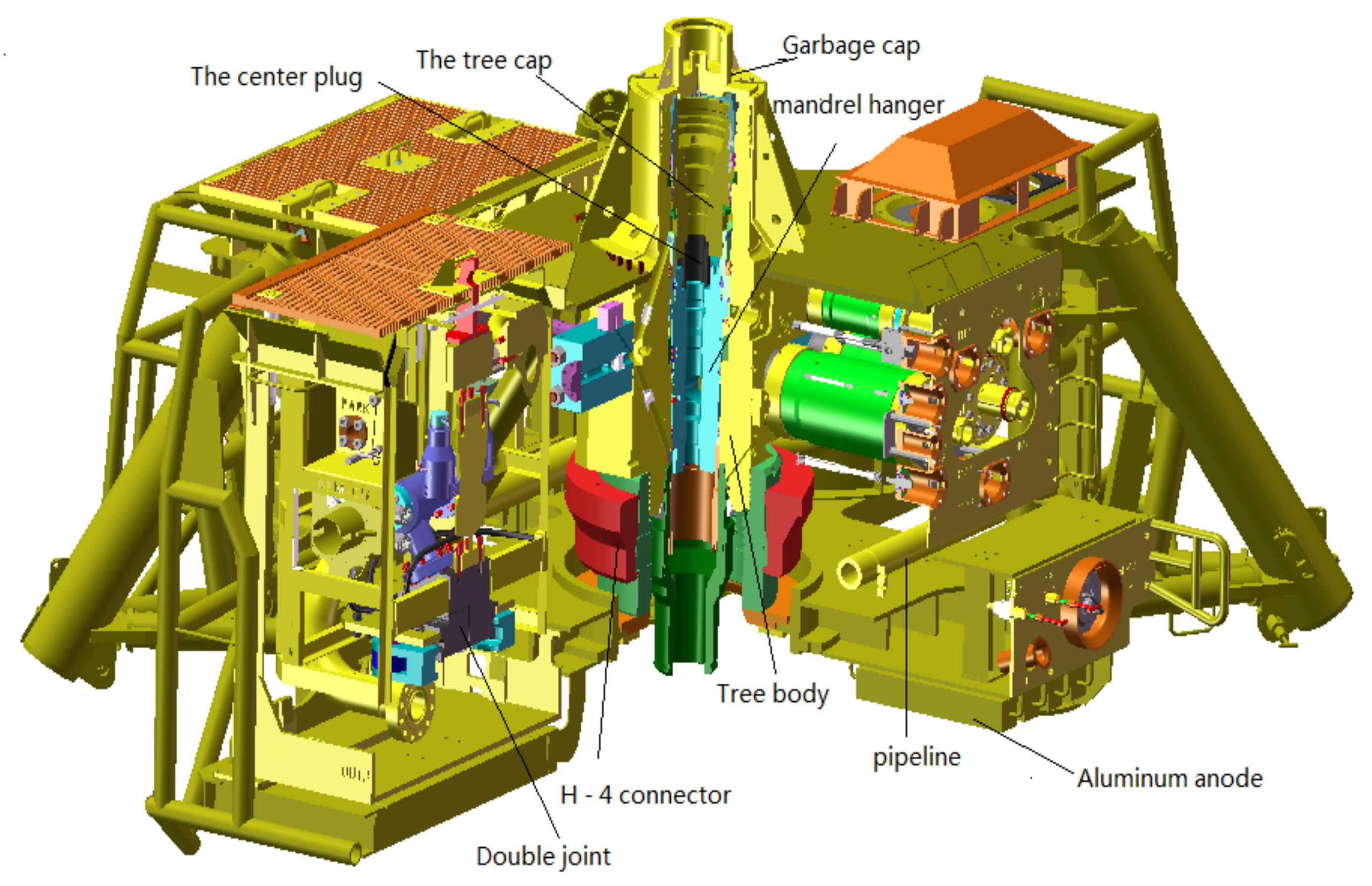
Figure 1 shows a sectional view of the assembly of the submarine Christmas tree. As can be seen from the figure, the subsea tree body is central and plays an important role, connected to the wellhead with an H-4 connector. The tubing hanger is placed above the subsea tree body, and the fluid collected from the tubing hanger passes through various connectors and valve sets and finally is led to the external pipeline by the 4 inch pipe connector. The flow of specific fluids is shown in Figure 2.
The main components of the subsea tree are shown in Figure 1. The H-4 connector is used to connect the subsea tree body to the wellhead. The tubing is mounted on the subsea tree body and communicates with the main production valve and the subsea tree body’s annular main valve. The vertical center hole of the tubing hanger is sealed with a center plug. On the upper part of the tubing hang is a built-in tree cap. On the upper part of the built-in tree cap is a garbage cap; its function is to prevent sediment from falling into it. The annular main valve in the subsea tree body is connected to the annular wing valve, connected to the annular span nozzle. Both the annulus spanning nozzles and the subsea tree body’s main production valves are connected to the production wing valve sets. The production wing valve set is connected to the two-hole connector inlet through the reducer (51/8″ to 41/16″) to the throttle valve in the reservoir performance monitor(RPM) module and then flows back to the outlet of the two-hole connector through the production isolation valve (PIV) to connect the 4 inch pipe connector through the connecting pipe 2.
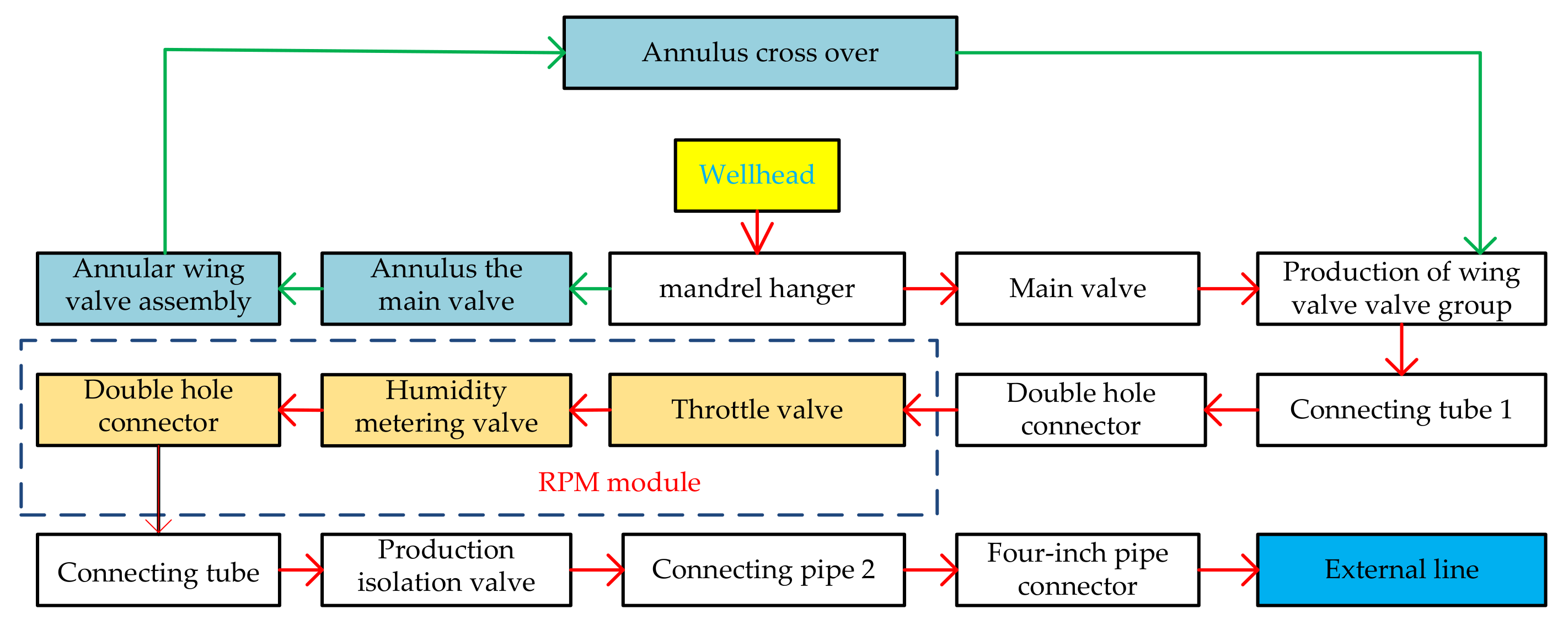
In the subsea tree, the flow map of the fluid is shown in Figure 2. It is locked and fixed between the subsea tree body and the wellhead through H-4 connectors. The fluid is led into the tubing, through the tubing down the hole, and then connected to the external pipeline through various valves, valve sets, connecting pipes and connectors on the subsea tree, and finally connected to the external pipeline through 4-inch pipe connectors.
3.2. Environmental Conditions of Subsea Tree Operation
Currently, subsea trees are designed to work in water depths ranging from 10 m to 3000 m. The ambient seawater temperature is estimated to be 0–30 degress, depending on the subsea tree’s operating area and the water depth. However, the inlet temperature of the gas–liquid mixture collected by the subsea tree is wide, ranging from −46 degress to 180 degress. The pressure of the collected fluid changes greatly due to the influence of crustal movement and the underwater environment, and the rated pressure of the subsea tree can be as high as 103.5 MPa. The composition of the fluid collected by the subsea tree is complex, which is the mixture of gas and liquid, and the proportion and material composition of the mixture isalso changing with the change of the exploitation stage.
Thus, it can be seen that the working environment of the subsea tree and the collected fluid are very complex. To study its vibration problem, some assumptions will be made on these environmental conditions and the composition of the collected fluid.
According to the current engineering requirements, it is assumed that the working water depth of the subsea tree in this paper is 150 m, the ambient seawater temperature is 20 degress, the inlet temperature of the gas–liquid mixture collected by the subsea tree is 103 degress, the pressure of the collected gas–liquid mixture is unknown, and the outlet pressure is ranging from 3.8 MPa to 12.1 MPa. The outlet pressure is derived from the working pressure of the gas storage equipment in the early and late stages of the oil and gas field being studied. In order to simplify the calculation model, it is assumed that all the gas–liquid mixtures collected are methane gas, and the methane collection rate is 4706 kg/s.
3.3. Modeling and Mesh Analysis of Subsea Tree Pipeline Fluid Domain
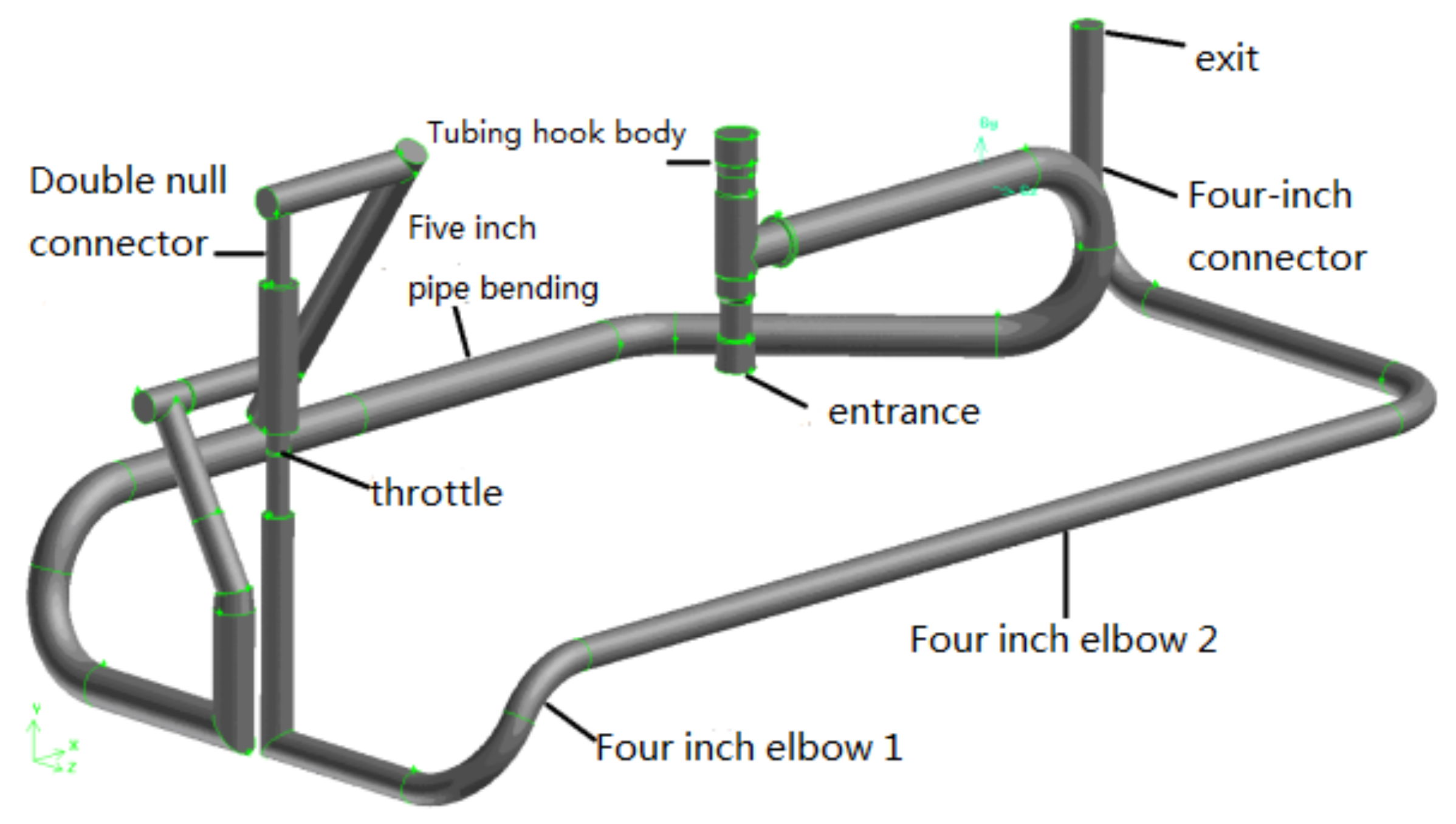
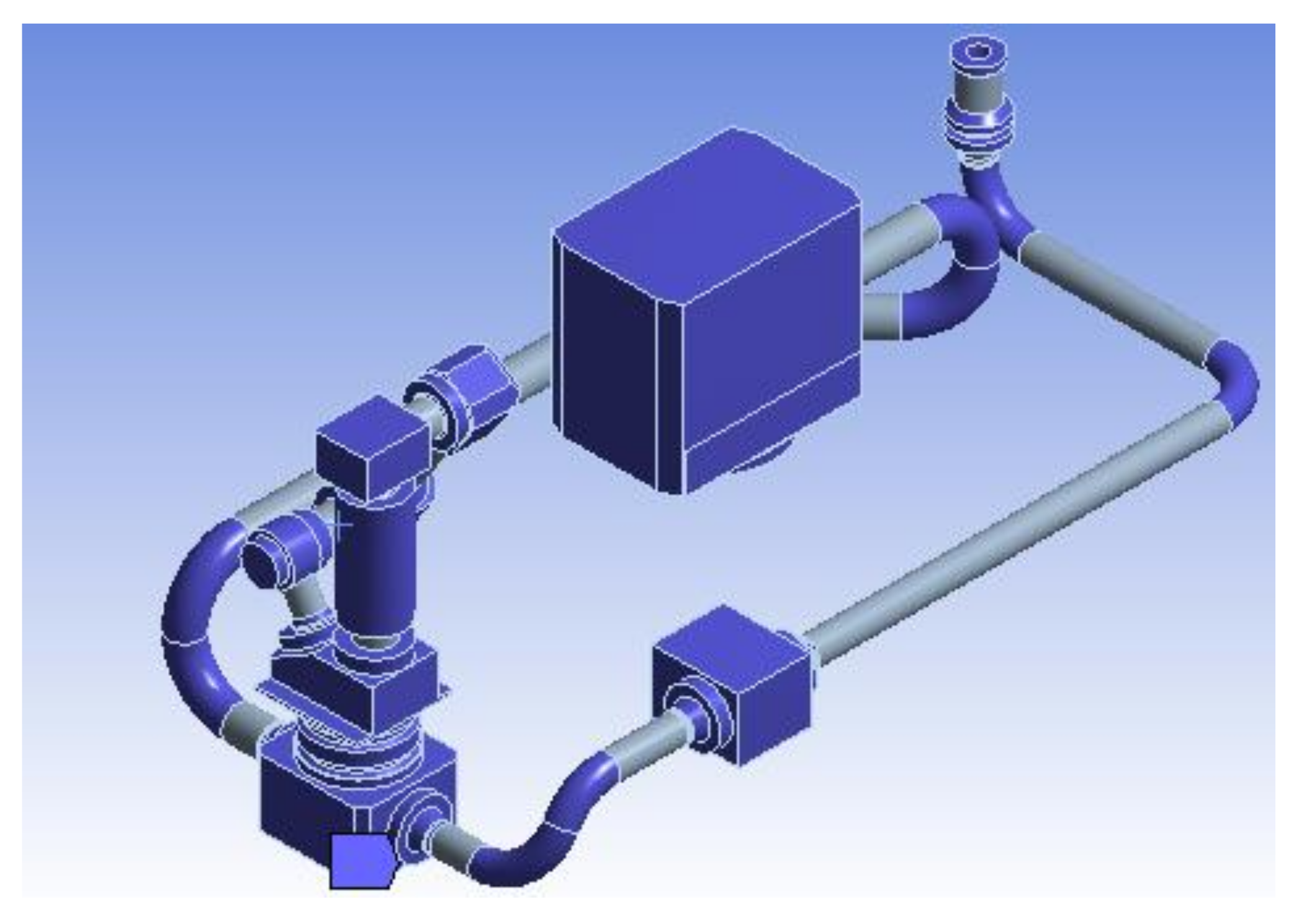
The overall flow field model of the subsea tree wasbuilt on the pipe wall of the subsea tree, just like the body. The whole modeling process wascompleted in GAMBIT. Figure 3 is a simplified diagram of the overall flow field of the underwater Christmas tree. It can be seen from the figure that the fluid flows in from the inlet at the lower end of the pipe and finally flows out from the outlet at the upper end.
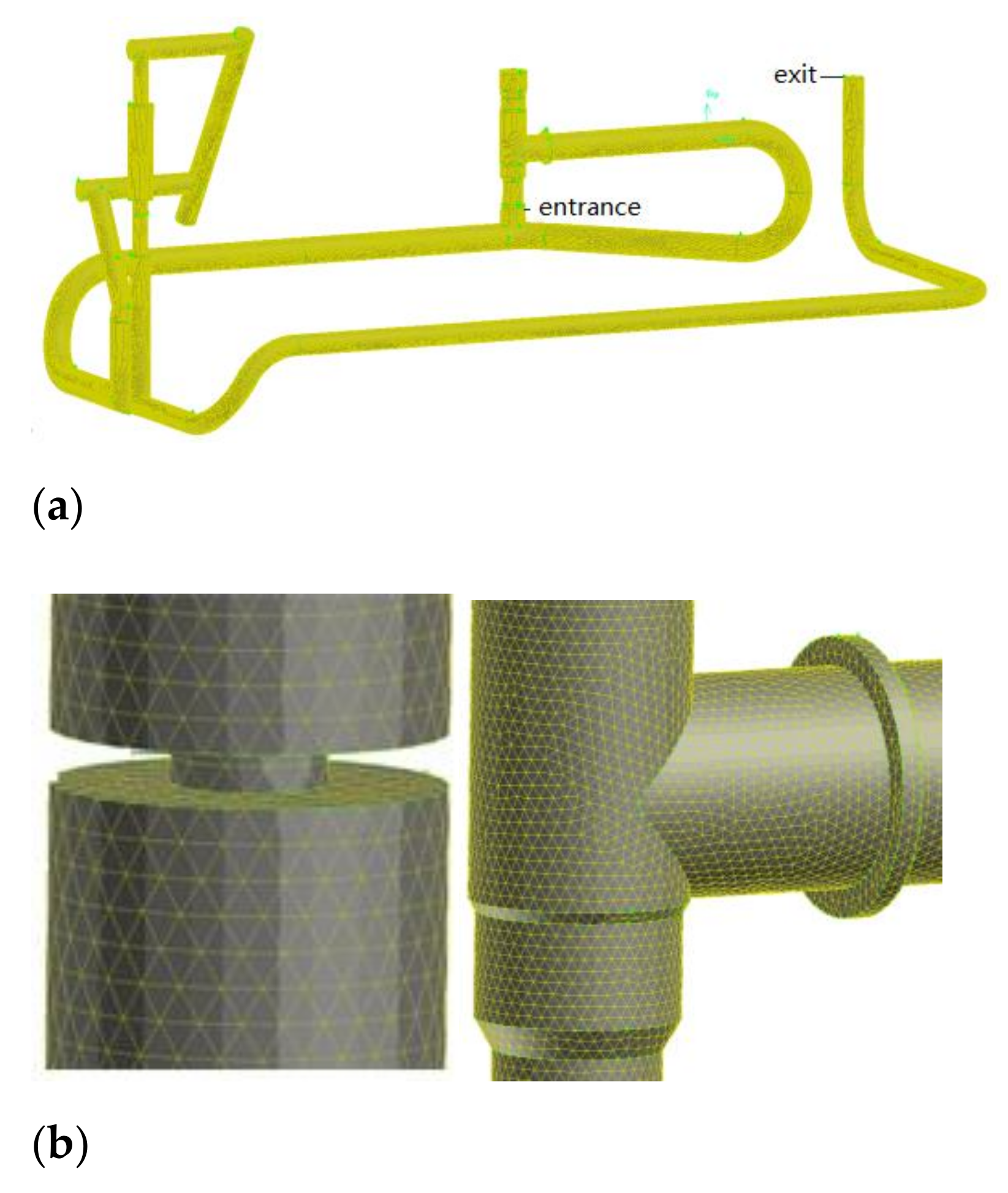
The mesh wasdivided in GAMBIT, and the fluid domain wasdivided into 2,381,521 tetrahedral elements. Figure 4a is the overall schematic diagram of meshing. Figure 4b is a partially enlarged view of the grid division. It can be seen from the local enlarged image that the mesh division of the flow field is dense, neat and uniform, and the mesh division can meet the requirements of numerical simulation.
3.4. Fluent calculation results and analysis
After the subsea treewasmodeled, it wasnecessary to set the flow field parameters of the subsea tree to collect oil and gas in the Fluent software. The fluid collected by the subsea tree studied in this paper wasmethane, and the parameter settings in the flow field are shown in Table 1.
3.5. Fluent Calculation Results and Analysis
The flow field under the two conditions was numerically simulated. After the analysis, the results related to velocity (the unit is m/s) and pressure (the unit is MPa) were shown. The specific analysis results are shown in Figure 5, Figure 6, Figure 7, Figure 8, Figure 9 and Figure 10.
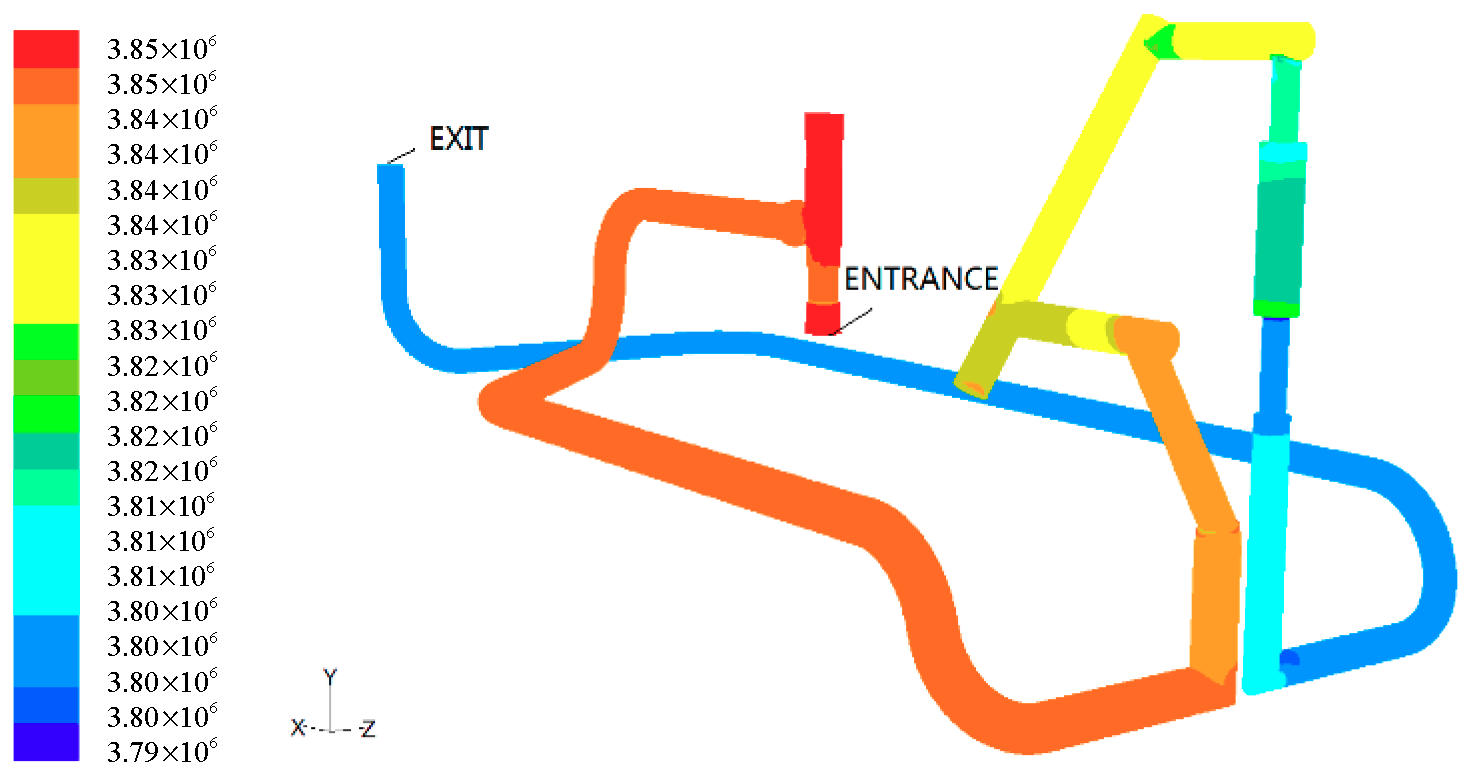
Figure 5 shows the pressure cloud diagram of the subsea tree’s overall flow field under working condition 1. The maximum pressure wasconcentrated before the throttle valve; this is because of the throttle valve that the pressure increases. The minimum pressure was 3.8 MPa concentrated between the metering valve and the outlet. It can be seen from the figure above that the pressure decreased from the inlet to the outlet. In the straight pipe, the pressure does not change much. At the bend and the diameter—especially at the right-angle bend—the pressure changed, possibly due to turbulence, but the pressure changed little from the inlet to the subsea tree’s outlet. As can be seen from the diagram, the whole tree fluid pressure presented three obvious changes. This was due to the fluid through the throttle valve and the metering valve interfering with decreasing the stress transfer. After the valve sets the pressure in a stable state, this way of easily decreasing the pass pressure is not stable, so it is prone to vibration and measurement at the throttle valve.
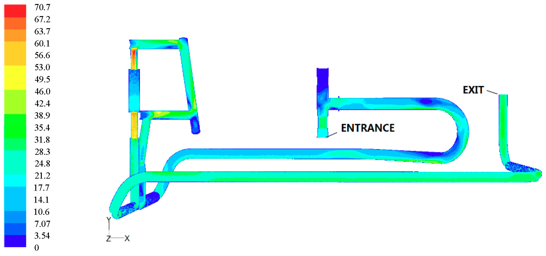
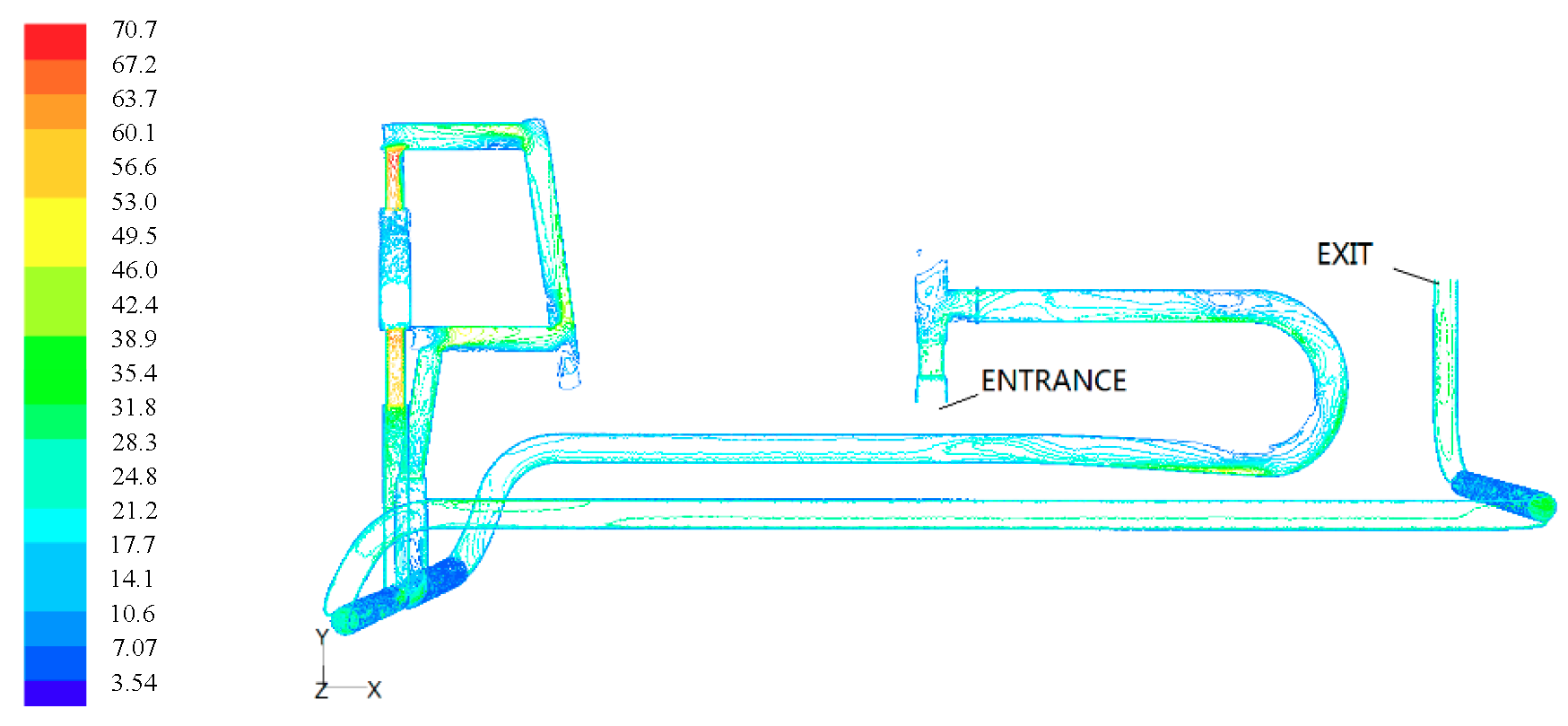
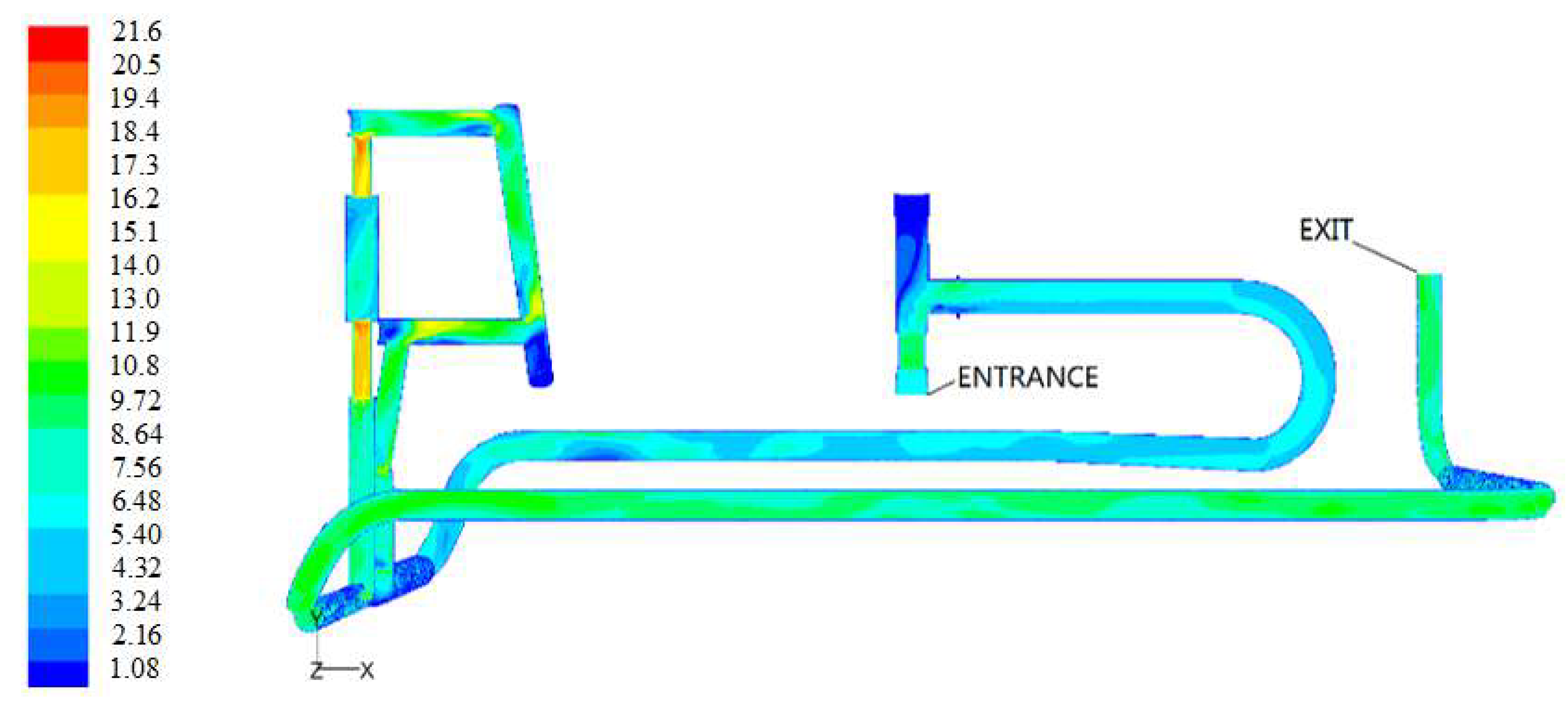
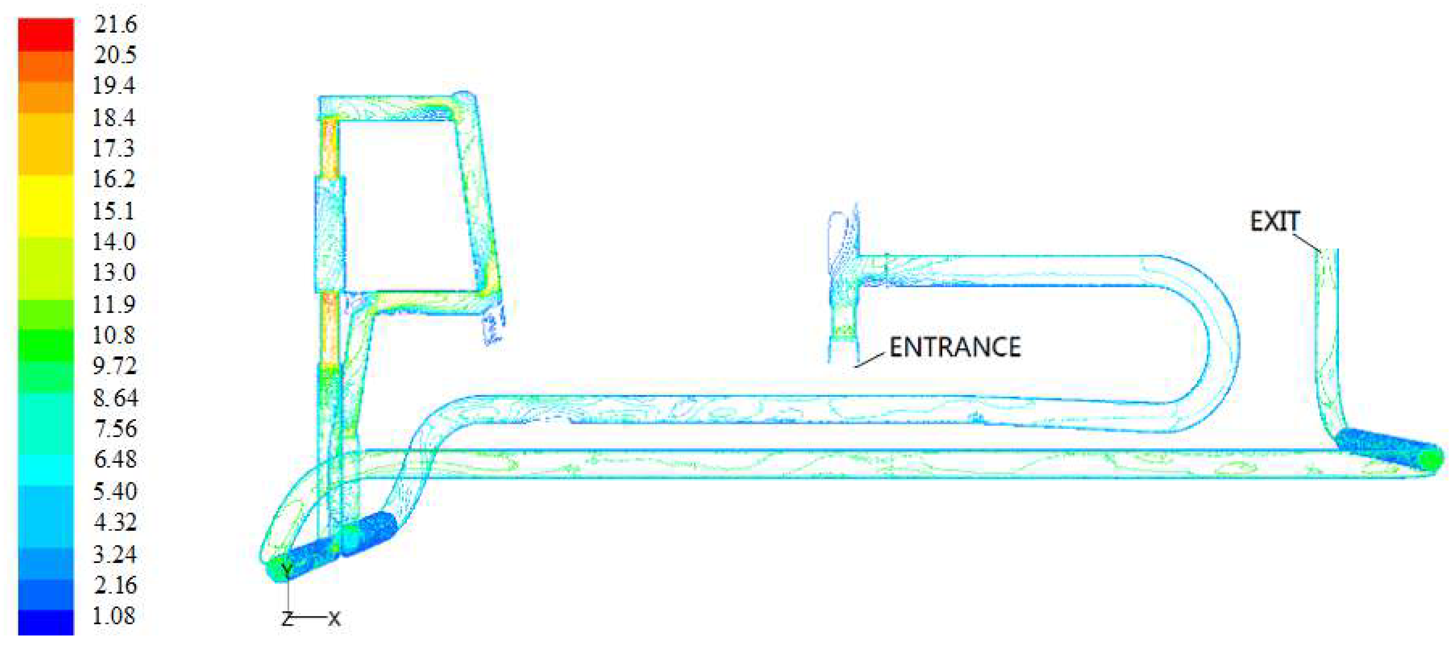
Figure 6 shows the velocity cloud diagram of the overall flow field of the structure under working condition 1. The maximum velocity in the fluid domain wassimilar to the analysis result of the flow field of the tree body. It can also be seen from the figure that most of the fluid is in a low-velocity state. Figure 7 shows the velocity contour of working condition 1. At the straight pipe, the streamline wasrelatively uniform without turbulence, while at the bend and the variable diameter, especially at the right-angle turn, the streamline became disorderly, which wascaused by turbulence.
It can be seen from the figure that the local enlarging of the velocity peaksat the throttle valve and the metering valve. The fluid velocity at these two places wasvery fast. Corresponding to the pressure neograms, they werethe places with thehighest incidence of pipeline vibration.
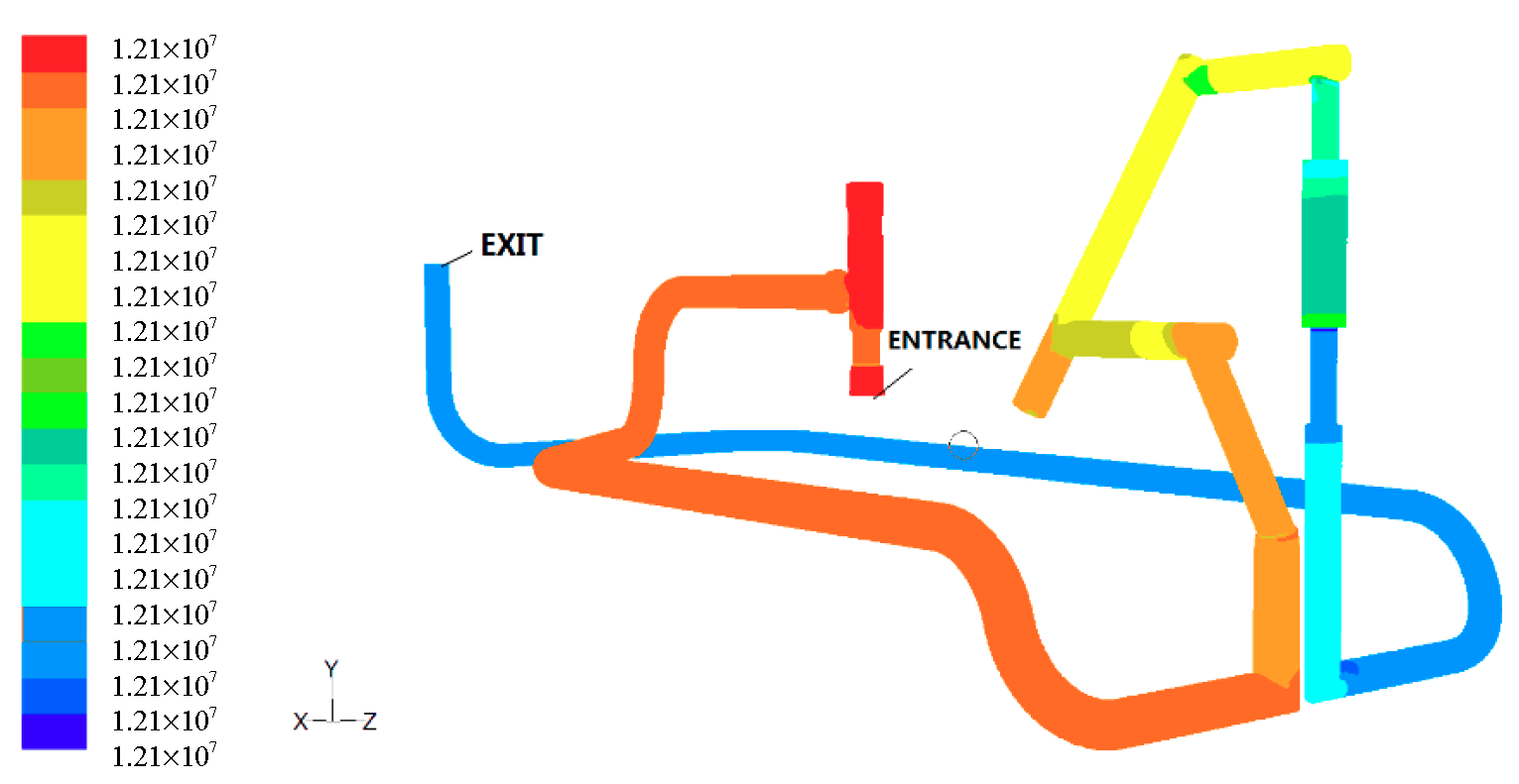
Figure 8 shows the pressure cloud diagram of the overall flow field of the structure under working condition 2. It can be seen from the above figure that, similar to working condition 1, the maximum pressure wasconcentrated before the throttle valve. The pressure behind the throttle valve wasstable at about 12.1 MPa, and the parts with pressure differenceswereprone to vibration. In the straight pipe, the pressure didnot change much. At the bend and the diameter, especially at the right-angle bend, the pressure changed, possibly due to turbulence, but the pressure changed little from the inlet to the outlet of the tree.
In thepartial enlargement of the pressure cloud at the throttle valve and metering in the figure, it can be seen that the fluid pressure at the throttle valve underwent a great change, which wasthe high-frequency of pipeline vibration.
Figure 9 shows the velocity cloud diagram of the overall flow field of the structure under working condition 2. The maximum velocity in the fluid domain was smaller than that in working condition 1 due to pressure difference and was similar to the flow field analysis results of the tree body. As can be seen from the figure above, most of the fluid was in a low-velocity state. Figure 10 shows the velocity contour of working condition 2. At the straight pipe, the streamline was relatively uniform without turbulence, while at the bend and the variable diameter, especially at the right-angle turn, the streamline became disorderly, and turbulence may occur.
From the partial enlargement of the velocity cloud at the throttle valve and metering valve, it can be seen that the fluid velocity in these two places is very fast, especially at the throttle valve, where the velocity reaches the maximum, which can easily lead to turbulence and vibration. The calculation results are shown in Table 2.
Table 2 summarizes the maximum and minimum pressure andmaximum and minimum speed under the two working conditions. Although the two working conditions were different in value, the section prone to vibration was the same, so the protection of the vibration section should be strengthened in the actual production.
4. Two-Way Fluid–Structure Coupling Analysis of Subsea Tree Pipeline
In this paper, the system coupling module of Ansys Workbench 16.0, a finite element software, wasused. This module can be coupled withfluent [35] with Ansysmechanical to realize the goalof two-way fluid–structure coupling analysis of the subsea tree body. In order to analyze the interaction of bidirectional fluid–structure, the transient solver was selected for the fluid analysis. In the solid analysis, the transient dynamics module was used, which couldanalyze the dynamic response of the structure during load changes. The boundary conditions of the fluid domain module and solid domain module were set in their respective modules, as shown in Table 3, and the coupling analysis was carried out in the system coupling module.
The main goal of computer-aided engineering (CAE) analysis wasto study the flow field distribution and vibration characteristics of subsea trees under two different working conditions. In order to reduce the calculation time, the geometric model of the subsea tree was appropriately simplified without affecting the calculation results. Some minor and small parts were eliminated. For example, the bolt holes around the valve block for fixing were simplified, and the chamfers at the corners of the body shell were simplified. Then, the simplified subsea tree model had meshed. Finally, the fluid–solid coupling calculation and analysis of the subsea tree pipeline were carried out.
The overall simplified subsea tree model consisted of two parts: the fluid domain and the solid domain. Then the model in Fluent and Transient Structural was shared to complete the geometric matching of the flow field and the solid. An automatic method mixed with tetrahedron and hexahedron elements was selected to establish the boundary surface of the fluid domain, including the entrance and exit surface and wall surface. The system coupling module was combined with the Fluent and Transient Structural modules to establish the model of the whole subsea tree system, as shown in Figure 11.
4.1. Modal Calculation Analysis of Underwater Subsea Tree
Through modal analysis, we can understand the subsea tree’s dynamic response under different load conditions, which can prevent the subsea tree from resonating or vibrating at a specific frequency in the actual working environment, and it is also conducive to control in the actual working environment. The overall modal analysis of the underwater subsea treeusedatwo-way fluid–solid coupling method. The fluid pressure calculated by this method wastransferred to the static structural module as a load item. The gravity field, external pressure and the variable diameter were added in the static structural fix constraints at the position, the right-angle elbow and the connecting device, and then the calculation time and the number of steps were set. Finally, the result calculated by Static Structuralwastransferred to the subsea tree module as a load term, and the first six modes of the structure weretaken to calculate its frequency mode under two working conditions, as shown in Figure 12 and Figure 13.
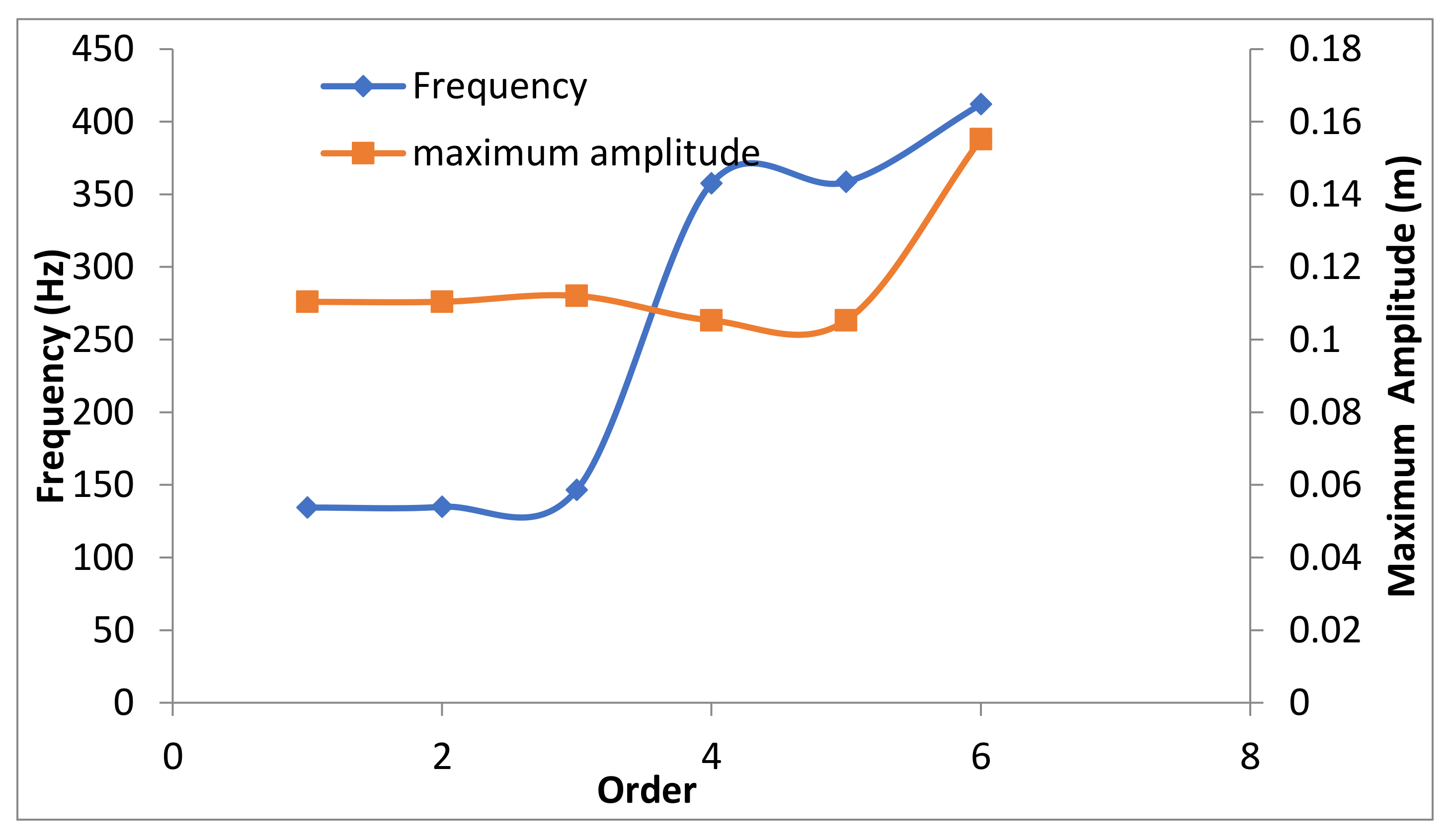
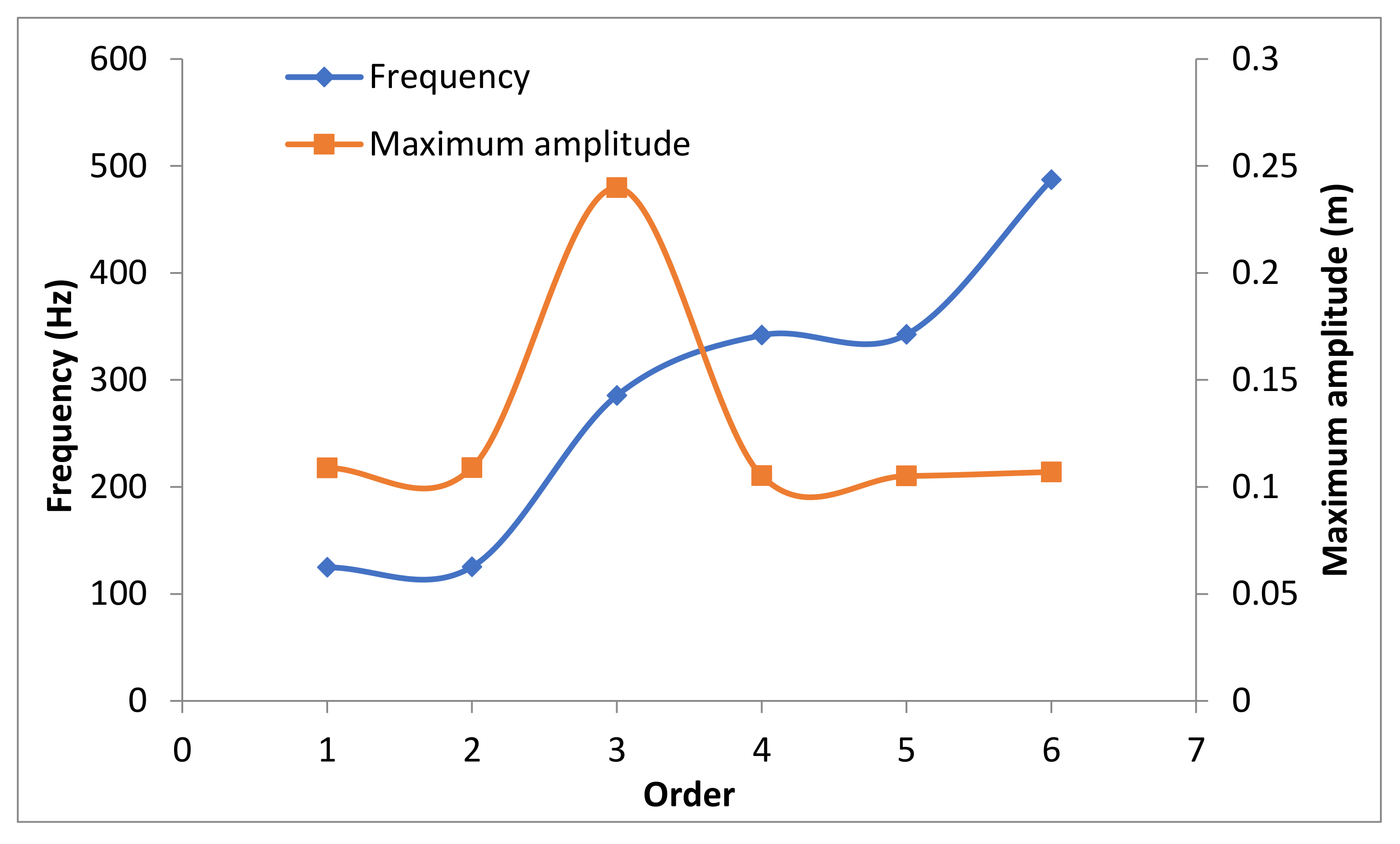
Figure 12 reflects the first six-order modal deformation cloud diagram of the overall operating condition 1 of the underwater subsea tree. From the dynamic display in the subsea tree module, it can be seen that the first-order mode showed that the structure wasunder the external influence of 134.37 Hz. The long straight pipe section of the second half of the lower subsea tree vibrates in a plane passing through the oz axis. The maximum vibration amplitude of 0.11038 m occurred in the middle section of the long straight pipe section, and the amplitude decreased from the middle to the two sides, the sixth stage. The modal performance wasthat under the external influence of 411.95 Hz. The long straight pipe section of the first half of the underwater subsea treewas vibrating in a plane passing through the z-axis. There was stretching in the z-axis direction, that was, the long straight pipe axial direction. Vibration, the maximum vibration amplitude of 0.15513 m occurred at a local position in front of this long straight pipe section, and the amplitude was more evenly distributed at this long straight section.Combining the above six-order modes, we could see the first-, second-, fourth-, and fifth-order modal deformation occur in the long straight pipe section in the second half of the overall structure. The third and sixth-order modal deformation occurred in the straight pipe section in the first half of the overall structure, and the maximum amplitude was above 0.1 m. Therefore, at these vibration frequencies, the long straight pipe was a weak and easily damaged section.
Figure 13 shows the first six-order modal deformation cloud diagram of the overall operating condition 2 of the underwater subsea tree. The third-order mode shows that the structure was under the external influence of 285.39 Hz, and the long straight pipe section of the first half of the overall underwater subsea tree passes through the z-axis. The vibration occurs in a plane, and there was tensile vibration in the z-axis direction, the long straight pipe’s axial direction. The maximum vibration amplitude of 0.23979 m occurred at a local position behind the long straight pipe section, and the amplitude goes from here to both sides decreased. Summing up the above six-order modes, it can be seen that the first, second, fourth, and fifth-order modal deformations occurred in the long straight pipe section in the second half of the overall structure, and the third and sixth-order modal deformations occurred in the straight pipe section of the first half of the overall structure. The pipe section and the maximum amplitude wereabove 0.1 m, so at these vibration frequencies, the long straight pipe section was weak and easily damaged.
Based on the above two working conditions, the calculation results of working condition 1 and working condition 2 were similar. The first, second, fourth, and fifth-order modal deformations occurred in the long straight pipe section in the second half of the overall structure, and the third and sixth-order modal deformations occurred. The modal deformation occurredin the straight pipe section of the first half of the overall structure, and the maximum amplitude is above 0.1 m. Therefore, in actual work, we should strengthen the weak section’s protection, that is, the long straight pipe section, and fix it at regular intervals. Measures, especially to strengthen the constraint treatment at the point where the maximum amplitude occurs.
4.2. Thermal Analysis of the Subsea Tree
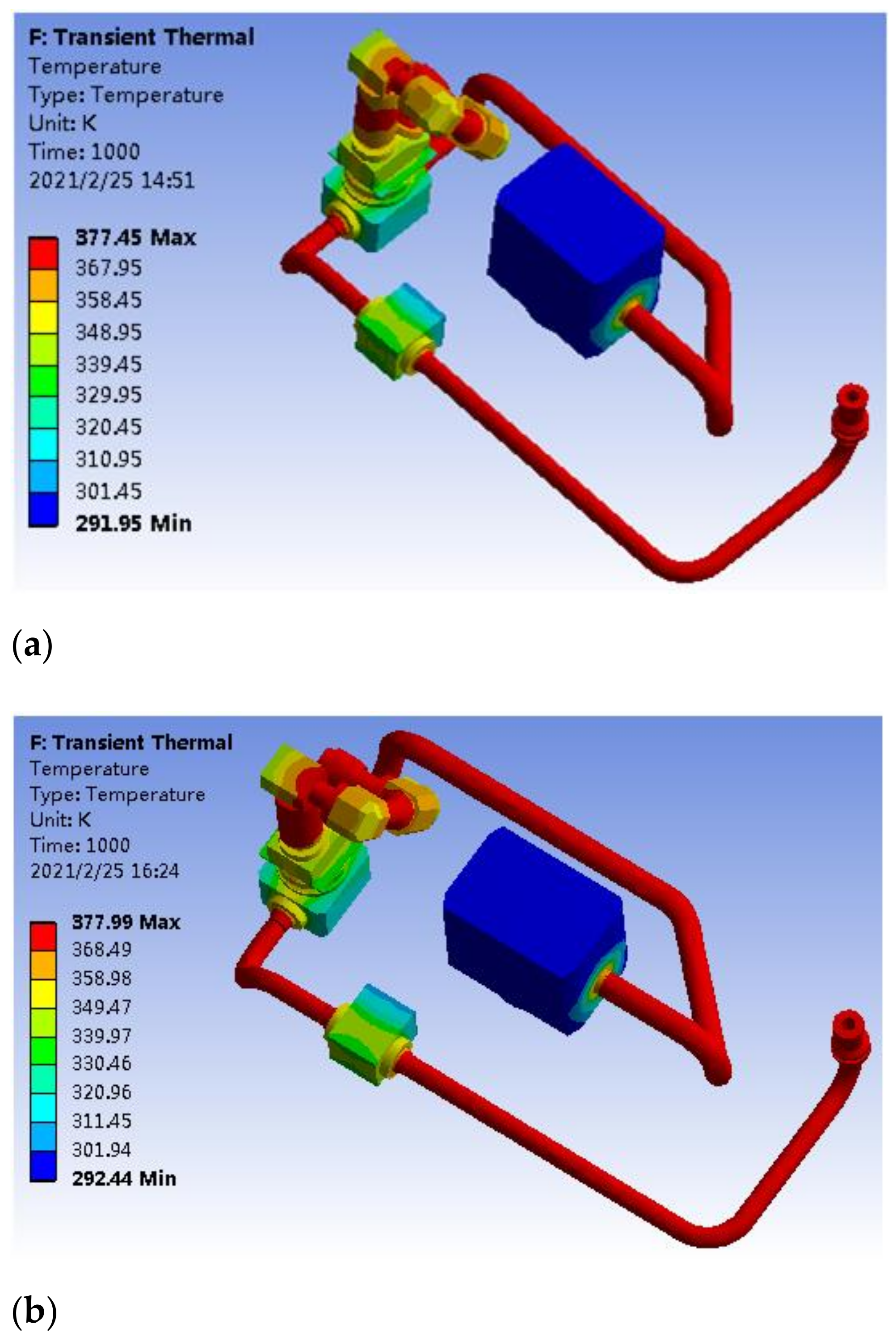
In this analysis, we transferred the Fluent solution into the two-way fluid–structure coupling to the setup of transient thermal. The finite element model in transient thermalwas shared with the model of the two-way fluid–structure coupling. The fluid domain temperature in the two-way fluid–structure coupling was loaded into transient thermal as a load term. In the imported temperature, the selection of the loading surfacewas consistent with the coupling interface, and the wall surface of the structure in contact with the fluid was selected. After setting the calculation time and the number of steps, the calculation was started, and we calculated the temperature distribution under the two working conditions. The calculated temperature distribution cloud chart is shown in Figure 14 and Figure 15.
Figure 14a shows the temperature distribution diagram of the subsea tree structure under working condition 1. It can be seen from the figure that the highest temperature was 377.45 K andthe lowest temperature was 291.95 K. In Figure 14b; it wasshown that the highest temperature was 377.99 K, the lowest temperature was 292.44 K. The temperature distribution of these two environmental conditions did not change much. The reason may be the fluid inlet temperature and outlet temperature settings were the same, but only the pressure difference.
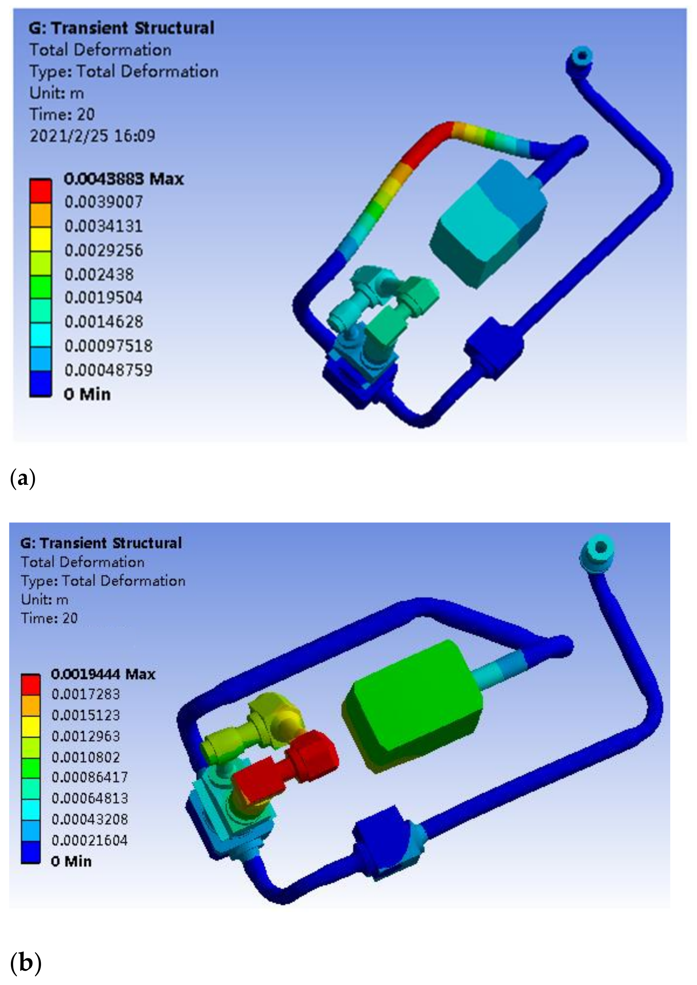
The temperature results calculated above were added as a load item to the Transient Structural to calculate the effect of temperature on the structure. The subsea tree structure displacement was calculated after setting the calculation time and the number of steps. The displacement cloud diagrams under the two working conditions are shown in Figure 15a,b.
Figure 15a shows the overall thermal stress and displacement cloud diagram under the condition of working condition 1. From the above figure, it can be concluded that the maximum displacement was 4 mm, and it was easy to occur at the bend of the pipeline. Figure 15b shows the overall thermal stress displacement cloud diagram under the condition of working condition 2. On the basis of working condition 1, constraints were added at the above-mentioned bend. From the figure above, it can be concluded that the maximum displacement was 1.9 mm, and the pipe wasessentiallynot affected by temperature.
5. Experimental Device and Scheme Design
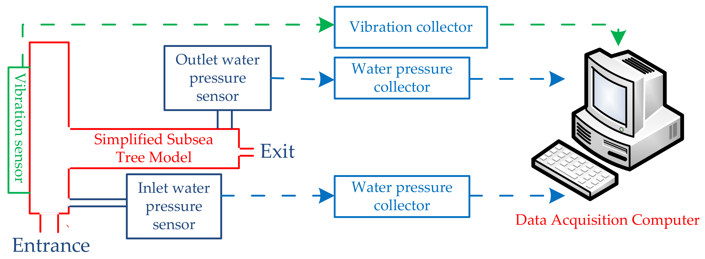
In this section, the subsea tree experiment was designed and carried out. The subsea tree model was simplified to a trigeminal pipeline similar to the fluid domain of the subsea tree body, and the flow field characteristics and modal modes under the action of fluid–solid coupling were studied. Specifically, a simplified subsea tree model was designed. The schematic diagram of the experiment is shown in Figure 16. The main experimental equipment included a water pressure sensor, vibration sensor, water pressure collector, and 24 V power supply. The 24 V power supply was used to provide voltage to the smart meter for measuring water pressure. The water pressure sensor was used to measure the water pressure at the inlet and outlet of the trigeminal pipe. The vibration sensor used advanced digital filtering technology, which could effectively reduce external interference and improve the accuracy of measurement. The water pressure collector wasused to convert the analog water pressure signal of the water pressure sensor into a digital signal.
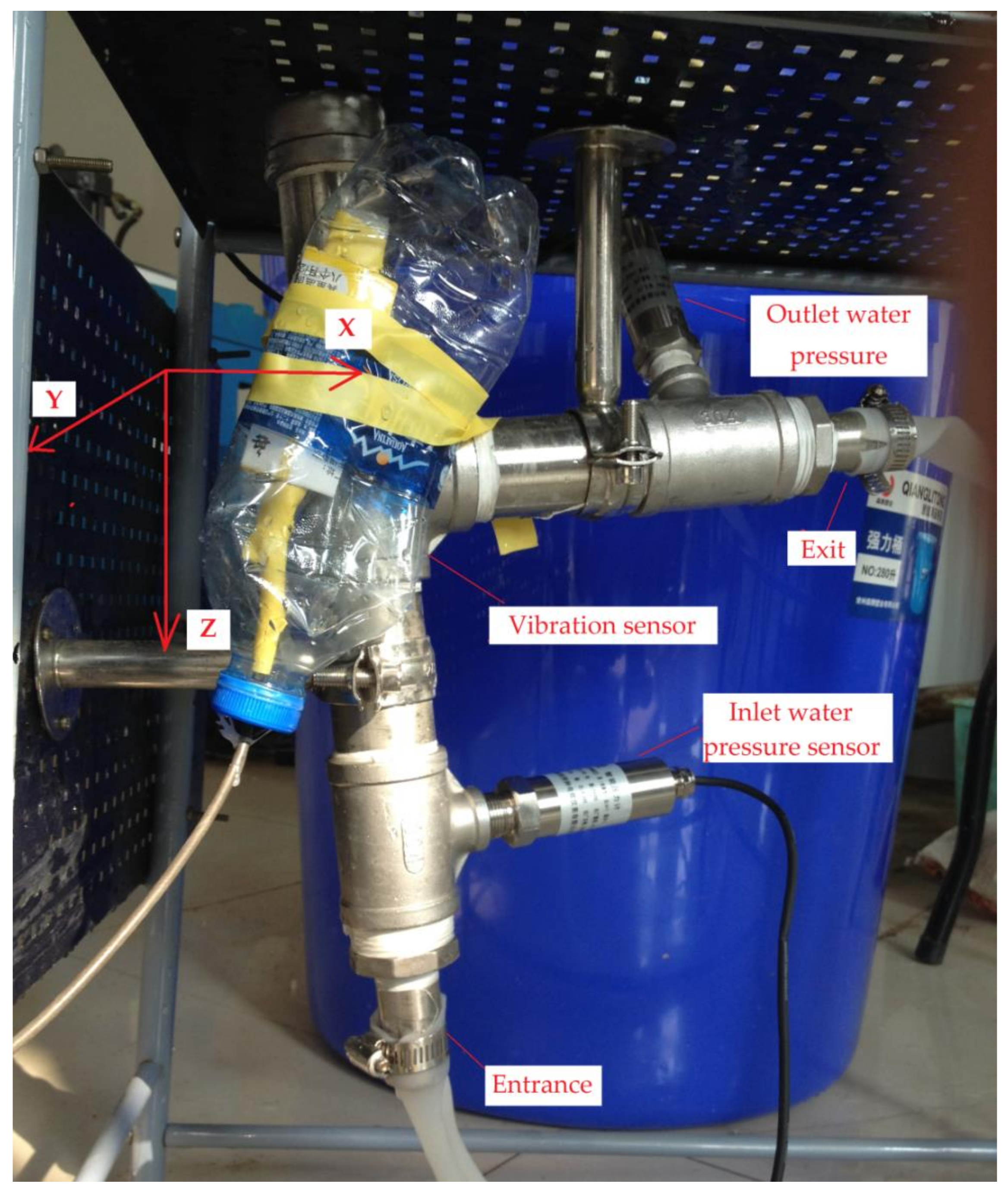
When the experimental design was completed, the water pressure sensor and vibration sensor were installed inthe simplified subsea tree model. The water pressure sensor and acceleration sensor were connected with the computer, and the data acquisition software parameters supported were set. This experimental device was installed on a shelf so that it could be put underwater as a whole for testing, as shown in Figure 17.
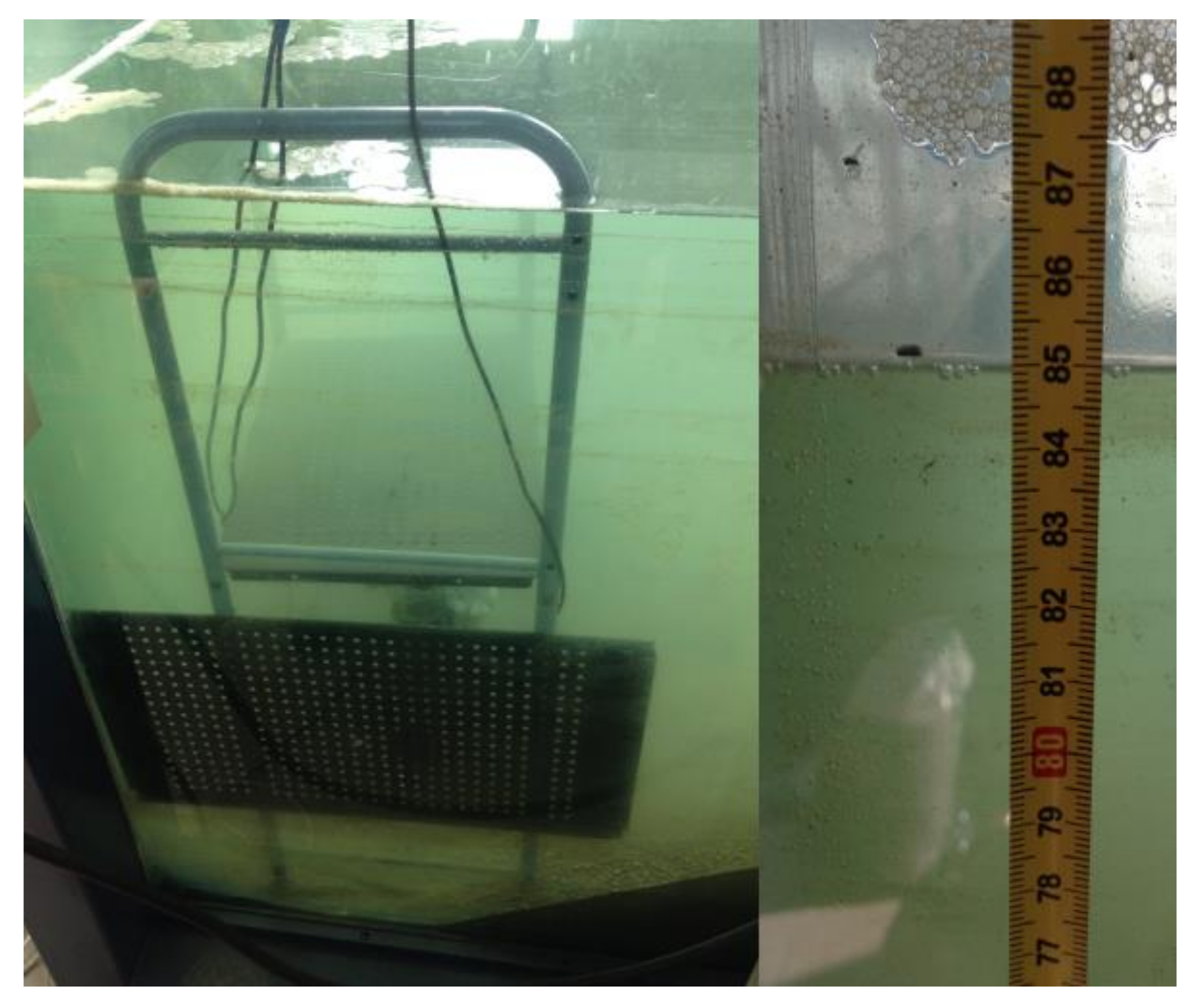
As shown in Figure 18, this experimental device was placed in a water tank with a water depth of 85 cm. The water inlet pipe was connected to the tap water pipe, and the water stop valve was opened to allow water to enter the trigeminal pipe system. The water pressure collector and vibration collector on the computer started sampling and recording experimental data. After collecting for some time, the collected data wereinitially analyzed, and then the reliability of the data was verified. The experimental process was repeated to obtain multiple sets of experimental data and reduce the acquisition device’s noise and errors.
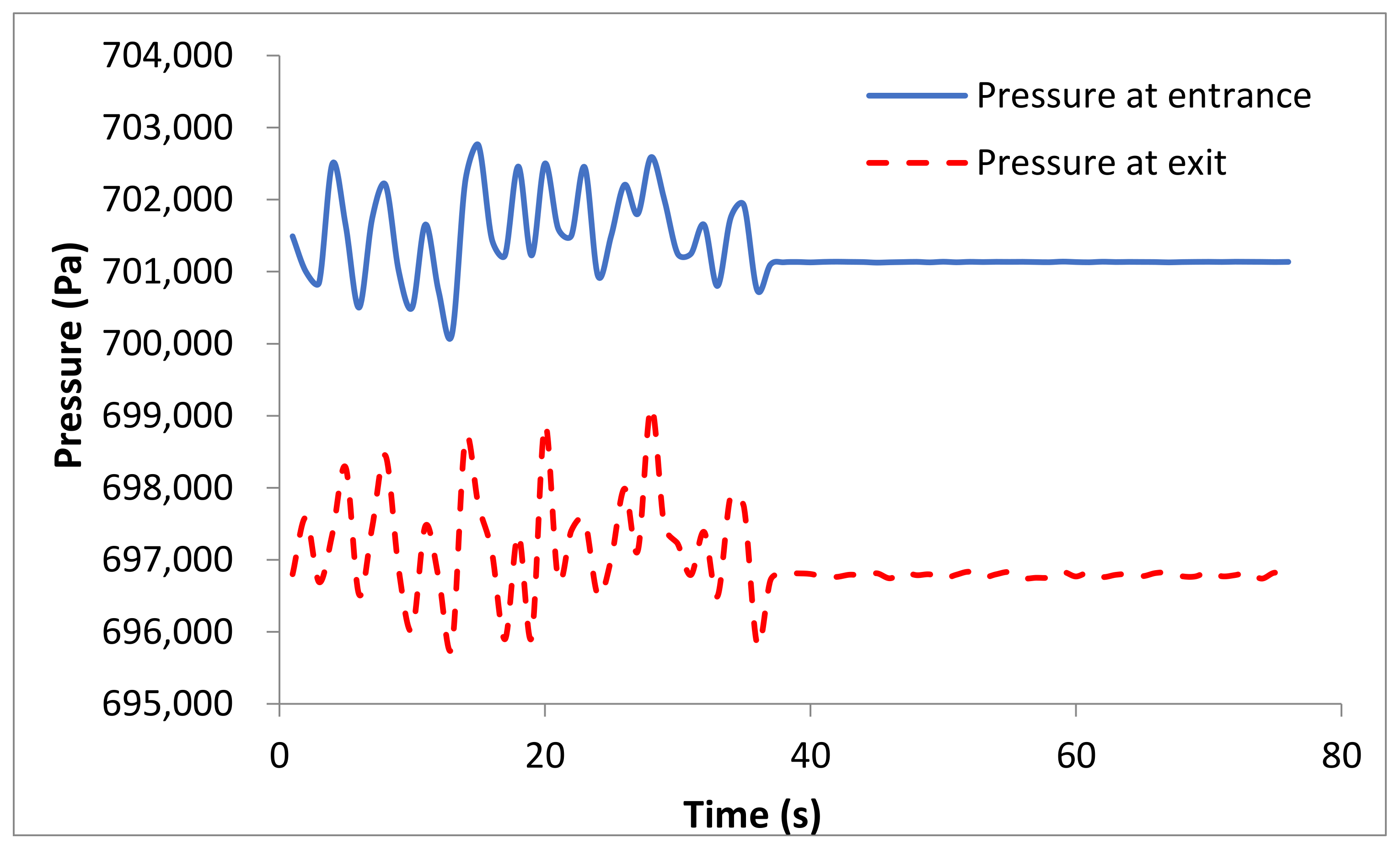
After the experiment of the simplified Subsea tree model was completed, the collected data were analyzed. It can be seen that the water pressure at the entrance was unstable at the beginning and then stabilized in Figure 19. The entrance pressure stabilized around 0.701 Mpa, and the exit pressure stabilized around 0.697 Mpa. Because the model built by the numerical simulation wassimplified, and there wasan error between the actual trigeminal pipeline and the pipeline in the boundary conditions set by the numerical simulation model, so the numerical simulation and the actual data weredifferent, but it waswithin a reasonable range.
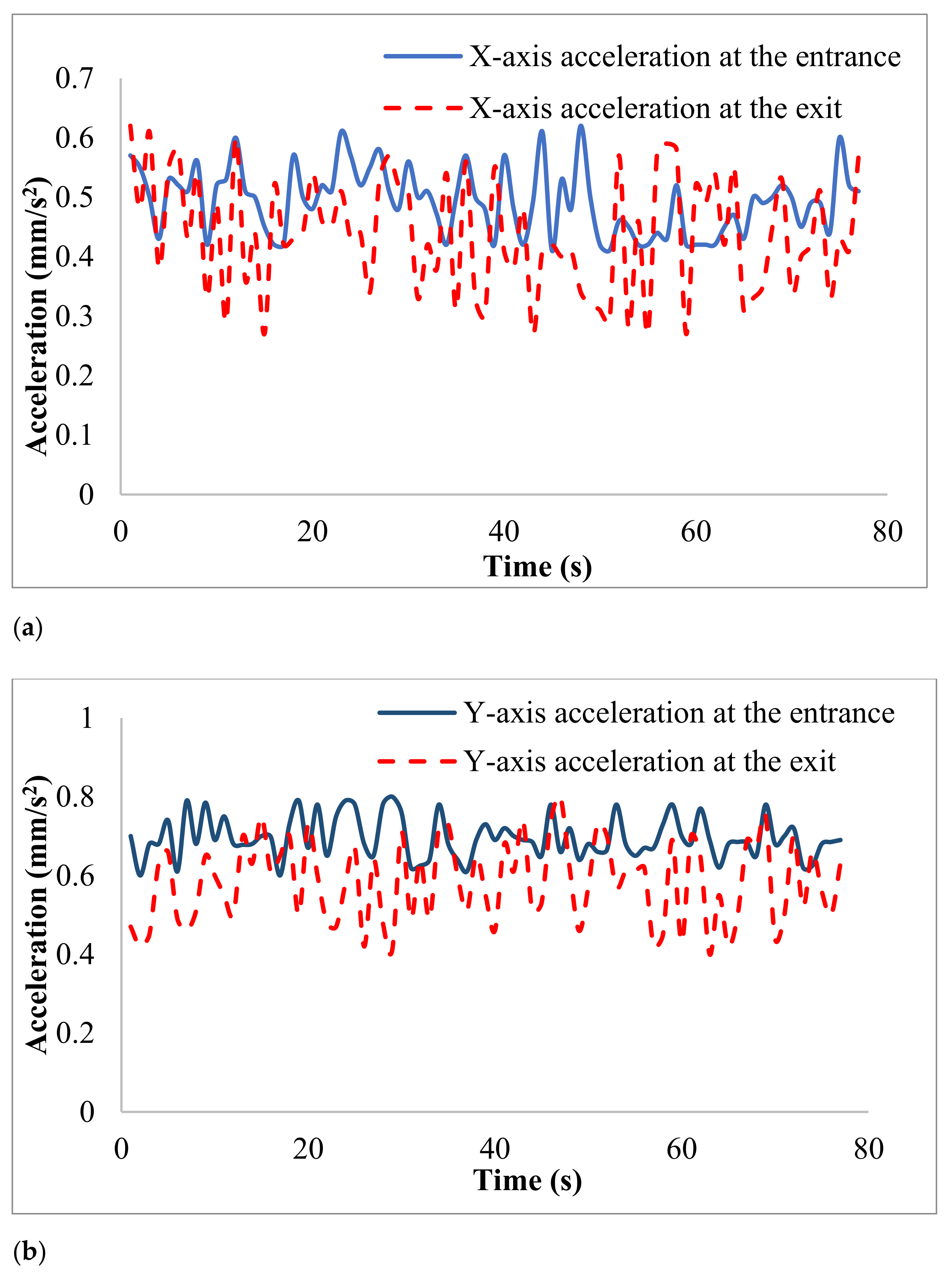
The acceleration data in three directions at the entrypoint from thevibrationsensor were recorded. Among these data, the time from opening the water stop valve to closing the water stop valve was selected from 5 s to 8 s, which was the most representative. According to the data collected during the period, the average x-axis acceleration was 0.53 mm/s2; the average y-axis acceleration was 0.71 mm/s2; the average z-axis acceleration was 0.135 mm/s2, as shown in Figure 20. The y-axis acceleration was the largest. The formula could be obtained, represents the distance the water flows through, represents the initial velocity of the water flow, represents the time, and represents the acceleration of the water flow, the maximum amplitude at the entrance pointwas 0.4 mm, and the smallest third-order mode maximum vibration amplitude was 0.48 mm; that was, the actuallymeasured amplitude did not exceed the maximum vibration amplitude calculated by the numerical simulation.
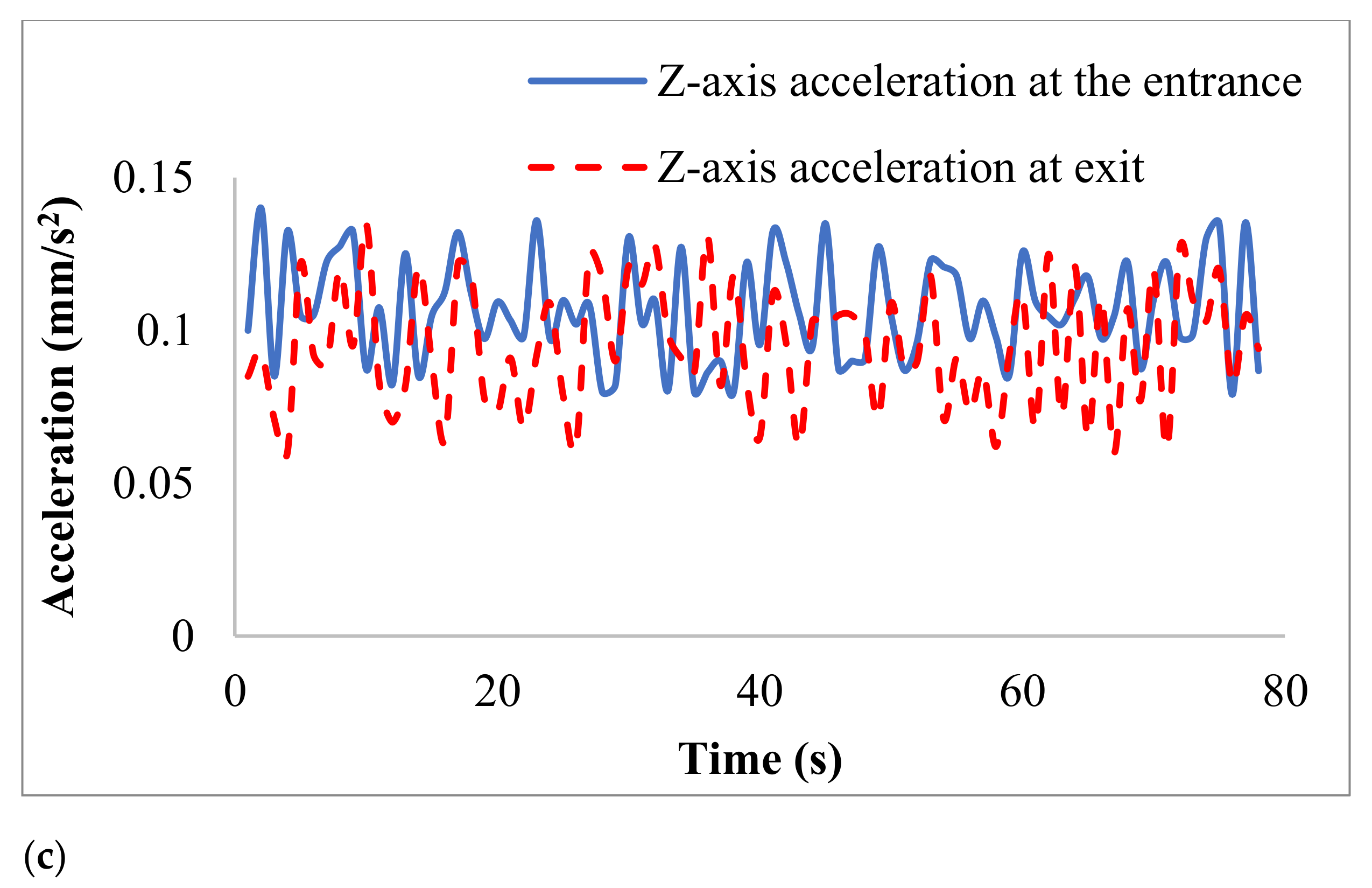
The average x-axis acceleration at the entrance was 0.51 mm/s2 and the average x-axis acceleration at the exit was 0.46 mm/s2, both of which were smaller than the average x-axis acceleration at a right-angle corner. The average y-axis acceleration at the entrance was 0.69 mm/s2, and the average y-axis acceleration at the exit was 0.59 mm/s2, both of which were smaller than the average y-axis acceleration at a right-angle corner. The z-axis acceleration line graph at the exit and the entrance, the average z-axis acceleration at the entrance was 0.107 mm/s2, and the average z-axis acceleration at the exit was 0.099 mm/s2, both of which were smaller than the average z-axis acceleration at a right-angle corner. In summary, the vibration amplitude at the right-angle corner of the trigeminal pipeline was the largest, which verified the correctness of the conclusions that the fluid in Section 3 and Section 4.
6. Conclusions
This paper takes the underwater subsea tree pipeline system as the research object and conducts two-way fluid–solid coupling analysis and modal analysis on it. The simulation experiment results showed that: the fluid velocity at the throttle valve and metering valve was very fast, the turbulence phenomenon was relatively serious, and it was easy to cause structural vibration.The finite element software Workbench 16.0 was used to analyze the tree modes, and it was found that the long straight pipe section was most affected by vibration at a specific frequency.
In the actual exploitation process, due to the change of oil and gas pressure and output at the tree inlet, when oil and gas flow through the elbow, reducing pipe, branch pipe, valve, blind plate and other pipe components, the vibration of the underwater tree pipeline will be caused. Because fluid flows in the pipeline, when external conditions, such as the working pressure of the tree, the production, the size of the pipeline flow, or the curvature of the pipeline changes, the changes in the fluid velocity and pressure will cause the vibration and deformation of the pipeline system. The vibration of the pipeline will aggravate the local stress concentration. When the vibration reaches a certain degree and lasts for a long time, it will lead to the loosening and destruction of the underwater subsea tree pipeline, which will lead to the leakage of fluid and cause certain economic losses and major safety accidents. The fluid–solid coupling vibration of the pipeline system caused by the fluid flowing through the pipeline is the main cause of pipeline vibration. For the safe operation of subsea trees, this article proposes the following suggestions:
- There willinevitably be a bend, diameter, branch, valve and other pipe components in the subsea tree pipeline. The existence of these exciting sources will produce exciting forces. Pipe layout should strive to be simple, as far as possible to reduce unnecessary elbow, size and other easy-to-produce vibration force pipe fittings. At the turning point of the piping system, elbows with a large curvature radius should be used as muchas possible instead of elbows; inclined connections should be used instead of right-angle connections, and forward connections should be used. These measures can effectively reduce the mechanical vibration amplitude, thereby reducing the harm caused by vibration;
- Support stiffness is an important factor affecting the natural frequency of the pipeline. The stronger the brace’s stiffness, the more influence the stiffness of the bracewill haveon the natural frequency of the system. The lower the support stiffness, the lower the natural frequency value of the pipe system, and vice versa; the stronger the support stiffness, the higher the natural frequency. Therefore, when designing the support, the stiffness of the support should be large, and the mass of the support should be small, and the connection between the pipe and the support should be as rigid as possible;
- The vibration is increasedwhen the pressure change frequency of the tree air inlet is close to the natural frequency of the pipeline. Attention should be paid to the frequency obtained from the modal analysis to avoid resonance and to strengthen the fixation at large displacement. Where the vibration amplitude is the largest under the first six modes frequency, these frequencies should be avoided in practical work, and measures should be taken to strengthen the fixing of the top.
Author Contributions
Conceptualization, G.W. and X.W.; methodology, G.W. and X.Z.; software, G.W.; investigation, X.W.; resources, G.W. and D.S.; writing—original draft preparation, X.W. and X.Z.; writing—review and editing, G.W., X.W. D.S. and X.Z.; visualization, G.W. and X.Z.; supervision, G.W.; project administration, G.W.; funding acquisition, G.W. All authors have read and agreed to the published version of the manuscript.
Funding
This research was funded by the National Natural Science Foundation of China, grant number51309148.
Institutional Review Board Statement
Not applicable.
Informed Consent Statement
Not applicable.
Data Availability Statement
The data used to support the findings of this study are available from the corresponding author upon request.
Acknowledgments
The authors gratefully acknowledge the financial support from the NationalNatural Science Foundation of China.
Conflicts of Interest
The authors declare no conflict of interest.
References
- Rostami, S.; Sepehrirad, M.; Dezfulizadeh, A.; Hussein, A.K.; Goldanlou, A.S.; Shadloo, M.S. Exergy optimization of a solar collector in flat plate shape equipped with elliptical pipes filled with turbulent nanofluid flow: A study for thermal management. Water 2020, 12, 2294. [Google Scholar] [CrossRef]
- Ren, K.R.; Wang, D.Y.; Zhou, T.M.; Shen, D.C.; Chen, C.H. Current situation and development trend of offshore oil subsea equipment. China Pet. Mach. 2008, 36, 151–153. [Google Scholar]
- Yang, J.; Liu, S.J.; Zhou, J.L.; Yan, D.; Tian, R.R.; Li, C. Development of deepwater oil drilling and production engineering simulation test device. China Pet. Mach. 2011, 39, 1–3. [Google Scholar]
- Zhao, H.L.; Cheng, H.R.; Tian, H.P.; Duan, M.l.; He, T.; Tang, K. Design of key parameters of lowering tool of deepwater tree tubing hanger. China Pet. Mach. 2014, 42, 16–19. [Google Scholar]
- Gong, M.X.; Liu, Z.S.; Duan, M.L.; Wang, J.G.; Zhang, M.H. Analysis and research on the process of deep-sea underwater tree laying. China Pet. Mach. 2013, 41, 50–54. [Google Scholar]
- Zhang, S.; Lu, Y.; Weijiong, C.; Liu, X. Intelligence Study on Subsea Christmas Tree Industry Based on Patent Analysis. J. Inf. 2014, 6, 74–78. [Google Scholar]
- Zhu, G.L.; Zhao, H.L.; Duan, M.L. Design elements analysis of subsea control module underwater Christmas tree. Pet. Field Mach. 2013, 42, 1–6. [Google Scholar]
- Lu, P.W.; Yuan, X.B.; Ou, Y.J.; Luo, Y.G.; Yang, W.; Su, R.H.; Zhang, Y.W.; Zhang, C.Q.; Cai, B.P. Research on the development status of underwater for Christmas tree. Pet. Field Mach. 2015, 6, 6–13. [Google Scholar]
- FMC Technologies. Subsea [K/OL]. Available online: http://www.fmctechnologies.com/en/Subsea%Systems/Technologies/Subsea%Production%Systems/SubseaTrees.aspx (accessed on 21 February 2021).
- Samad, J. Subsea development of marginal deepwater fields. In Proceedings of the Offshore Technology Conference-Asia, Kuala Lumpur, Malaysia, 25–28 March 2014. [Google Scholar]
- Zhang, H.; Chen, Z.G.; Wan, B. Research on the structural strength and experimental verification methods of underwater Christmas tree. Mod. Manuf. 2017, 30, 142–143. [Google Scholar] [CrossRef]
- Wu, Y.F. The Comparison of Two Coupling Approaches on the Analysis of Two-Way Fluid-Solid Interaction; Tianjin University: Tianjin, China, 2009. [Google Scholar]
- Yang, Y.; Chen, Z.Y. Calculation and analysis on natural frequency of fluid structure interaction in aero-engine pipelines. Gas Turbine Test Res. 2010, 23, 42–46. [Google Scholar]
- Li, H.F.; Ai, Y. Solution of fluid-structure coupling problem based on ANSYS and redevelop. Electroacoust. Technol. 2011, 35, 19–21. [Google Scholar] [CrossRef]
- Tao, D.L.; Geng, Z.; Shi, P.G. Numerical simulation analysis and optimal design of lubricating oil pipeline vibration for 10-K-302C reciprocating compressor. Guangdong Chem. Ind. 2014, 8, 118–123. [Google Scholar]
- Yu, S.R.; Ma, L.; Yu, L. Analysis of dynamic characteristics of fluid-structure coupling in curved pipes conveying fluid. Noise Vib. Control 2015, 35, 43–47. [Google Scholar]
- Zhang, J.; Liang, Z.; Han, C.J. Fluid-structure coupling analysis of U-shaped liquid-filled pipe. Chin. J. Appl. Mech. 2015, 32, 64–68. [Google Scholar]
- Ye, H.L.; Shao, P.Z.; Chen, N. Dynamic analysis and parameters’ influences on fluid-structure interaction in a fluid-filled pipes system. J. Beijing Univ. Technol. 2015, 41, 167–173. [Google Scholar] [CrossRef]
- Cao, Y. Research on Vibration Mechanism of Gas-Solid Coupling Pipeline; Yanshan University: Hebei, China, 2016. [Google Scholar]
- Dou, Y.H.; Yu, K.Q.; Yang, X.T.; Cao, Y.P. Finite element analysis of fluid-structure coupling vibration of fluid-conveying elbows. Mach. Des. Manuf. Eng. 2017, 46, 18–21. [Google Scholar] [CrossRef]
- Zhang, X.M. Research on Vibration Characteristics of Fluid-Solid Coupling Indoor Water Supply Pipeline Based on ANSYS Workbench. Chongqing. Master’s Thesis, Southwest University, Chongqing, China, 2018. [Google Scholar]
- Bai, Y.C.; Xie, W.D.; Gao, X.F.; Xu, W. Dynamic analysis of a cantilevered pipeconveying fluid with density variation. J. Fluids Struct. 2018, 81, 638–655. [Google Scholar] [CrossRef]
- Xie, C.L.; Wang, Z.Y. Numerical simulation of fluid-solid coupling of L-tube gas-liquid two-phase internal flow-induced vibration. Pet. Mach. 2019, 47, 124–128. [Google Scholar] [CrossRef]
- Wang, F.M.; Xu, Z.L.; Wu, W.B.; Liu, S.J. Analysis of dynamic characteristics of straight pipes filled with liquid under pulse dynamic action. Noise Vib. Control 2013, 2, 11–14. [Google Scholar]
- Liang, J.S.; Su, Q.; Li, X.Y. Modal analysis of fluid-structure interaction bellows based on ANSYS/Workbench. Mach. Des. Manufact. 2013, 2, 91–93. [Google Scholar] [CrossRef]
- Shi, D.D.; Xie, W.Y.; Kong, G.; Liu, W.B.; Bie, Y.B. Finite element analysis of mechanical properties of seismic supports and hangers for building pipelines. Comput. Aided Eng. 2019, 28, 56–62. [Google Scholar] [CrossRef]
- Liu, H.G.; Kong, J.Y.; Li, G.F.; Wang, X.D.; Liu, Y.J. Vibration analysis and control of liquid-filled pipeline system. J. Hubei Univ. Technol. 2005, 20, 2–4. [Google Scholar]
- Zhang, L.X. iResearch on fluid-structure coupling vibration of pipeline. Adv. Hydrodyn. Res. 2000, 15, 3. [Google Scholar]
- Zhang, T.; Lin, Z.H.; Lin, T.; Zhang, H. Analysis of dynamic instability of fluid conveying pipeline under the action of internally excited oscillating attenuated flow. J. Vib. Shock 2021, 40, 3. [Google Scholar] [CrossRef]
- Guo, S.Q. Random Uncertainty Modeling and Vibration Analysis of Pipes Conveying Multi-phase Fluid; Zhejiang University: Hangzhou, China, 2014. [Google Scholar]
- Yang, K.; Zhang, L.X.; Wang, B.D. A symmetric model of liquid filled pipe in axial vibration. Res. Prog. Hydrodyn. 2005, 20, 8–13. [Google Scholar]
- Ren, J.T. Traveling wave method of pipeline fluid-structure coupling vibration. Chin. J. Appl. Mech. 2006, 22, 530–535. [Google Scholar]
- Ni, Z.L. Burst Pressure of Glass Fiber Reinforced Composite Pipe with Delamination Defect; Zhejiang University: Hangzhou, China, 2020. [Google Scholar] [CrossRef]
- Besbes, S.; Hajem, M.; Aissia, H.B.; Champagne, J.Y. Low reynolds number turbulence models to simulate the bubble plume behavior with the euler-euler method. J. Appl. Fluid Mech. 2021, 14, 1–10. [Google Scholar] [CrossRef]
- Siddiqui, N.A.; Chaab, M.A. A simple passive device for the drag reduction of an ahmed body. J. Appl. Fluid Mech. 2021, 14. [Google Scholar] [CrossRef]
Figure 1.
Drawing of the profile of subseatree assembly.

Figure 2.
Fluid flow route of the subseatree.

Figure 3.
Fluid domain model of the subsea tree.

Figure 4.
Analysis of subsea tree meshing. (a) Subsea treemeshing; (b) local mesh amplification of the throttle valve and tubing hanger body.
Figure 4.
Analysis of subsea tree meshing. (a) Subsea treemeshing; (b) local mesh amplification of the throttle valve and tubing hanger body.

Figure 5.
Pressure cloud diagram of working condition 1.

Figure 6.
Velocity cloud diagram of working condition 1.

Figure 7.
Velocity contour of working condition 1.

Figure 8.
Pressure cloud diagram of working condition 2.

Figure 9.
Velocity cloud diagram of working condition 2.

Figure 10.
Velocity contour of working condition 2.

Figure 11.
Schematic diagram of overall constraints.

Figure 12.
Modal analysis diagram of working condition 1.

Figure 13.
Modal analysis diagram of working condition 2.

Figure 14.
Overall temperature distribution cloud diagram for the subsea tree (a) under condition 1 and (b) under condition 2.
Figure 14.
Overall temperature distribution cloud diagram for the subsea tree (a) under condition 1 and (b) under condition 2.

Figure 15.
Overall temperature distribution cloud diagram for the subsea tree (a) under condition 1 and (b) under condition 2.
Figure 15.
Overall temperature distribution cloud diagram for the subsea tree (a) under condition 1 and (b) under condition 2.

Figure 16.
Experiment design forthe simplified subsea tree model.

Figure 17.
Schematic diagram of the subsea tree experiment assembly.

Figure 18.
The experimental device underwater for testing.

Figure 19.
Comparison of inlet and outlet pressure.

Figure 20.
Comparison of acceleration in each direction of entrance and exit. (a) x-axis acceleration; (b) y-axis acceleration; (c) z-axis acceleration.
Figure 20.
Comparison of acceleration in each direction of entrance and exit. (a) x-axis acceleration; (b) y-axis acceleration; (c) z-axis acceleration.


Table 1.
Setting of calculation parameters.
| Flow Field Calculation Method | Flow Regime | Turbulence Model | Y-axis Acceleration (m/s2) | Ambient Temperature (K) | Fluid Material | Solving Algorithm | Residual Accuracy | Number of Iterations (Times) |
|---|---|---|---|---|---|---|---|---|
| Implicit algorithm | Turbulence | k-Epsilon | −9.81 | 292.65 | CH4 | SIMPLE algorithm | 0.00001 | 500 |
Table 2.
Analysis of the calculation results.
| Operating Condition | Maximum Pressure (MPa) | Minimum Pressure (MPa) | Maximum Speed (m/s) | Minimum Speed (m/s) |
|---|---|---|---|---|
| Condition 1 | 3.8467 | 3.7907 | 70.7225 | 1.08 |
| Condition 2 | 12.1387 | 12.0931 | 21.5945 | 1.08 |
Table 3.
Setting for thesystem coupling module.
| Mesh Style | Algorithm Processing Type | Turbulence Modeling Type | Outer Wall Pressure (MPa) | Ambient Temperature (K) | Fluid Material | Solver Type |
|---|---|---|---|---|---|---|
| Tetrahedral mesh | Mechanical | k-Epsilon | 4.9 | 292.65 | CH4 | Fluent |
Publisher’s Note: MDPI stays neutral with regard to jurisdictional claims in published maps and institutional affiliations. |
© 2021 by the authors. Licensee MDPI, Basel, Switzerland. This article is an open access article distributed under the terms and conditions of the Creative Commons Attribution (CC BY) license (https://creativecommons.org/licenses/by/4.0/).
Share and Cite
MDPI and ACS Style
Wu, G.; Zhao, X.; Shi, D.; Wu, X. Analysis of Fluid–Structure Coupling Vibration Mechanism for Subsea Tree Pipeline Combined with Fluent and Ansys Workbench. Water 2021, 13, 955. https://doi.org/10.3390/w13070955
AMA Style
Wu G, Zhao X, Shi D, Wu X. Analysis of Fluid–Structure Coupling Vibration Mechanism for Subsea Tree Pipeline Combined with Fluent and Ansys Workbench. Water. 2021; 13(7):955. https://doi.org/10.3390/w13070955
Chicago/Turabian StyleWu, Gongxing, Xiaolong Zhao, Danda Shi, and Xiaodong Wu. 2021. "Analysis of Fluid–Structure Coupling Vibration Mechanism for Subsea Tree Pipeline Combined with Fluent and Ansys Workbench" Water 13, no. 7: 955. https://doi.org/10.3390/w13070955
Note that from the first issue of 2016, this journal uses article numbers instead of page numbers. See further details here.