
Porosity Models for Large-Scale Urban Flood Modelling: A Review


Research unit Urban & Environmental Engineering (UEE), Hydraulics in Environmental and Civil Engineering (HECE), University of Liège, 4000 Liège, Belgium
*
Author to whom correspondence should be addressed.
Water 2021, 13(7), 960; https://doi.org/10.3390/w13070960
Submission received: 24 February 2021
/
Revised: 23 March 2021
/
Accepted: 26 March 2021
/
Published: 31 March 2021
(This article belongs to the Special Issue Modelling of Floods in Urban Areas)
Abstract
:In the context of large-scale urban flood modeling, porosity shallow-water models enable a considerable speed-up in computations while preserving information on subgrid topography. Over the last two decades, major improvements have been brought to these models, but a single generally accepted model formulation has not yet been reached. Instead, existing models vary in many respects. Some studies define porosity parameters at the scale of the computational cells or cell interfaces, while others treat the urban area as a continuum and introduce statistically defined porosity parameters. The porosity parameters are considered either isotropic or anisotropic and depth-independent or depth-dependent. The underlying flow models are based either on the full shallow-water equations or approximations thereof, with various flow resistance parameterizations. Here, we provide a review of the spectrum of porosity models developed so far for large-scale urban flood modeling.
1. Introduction
Worldwide, climate evolution, population growth and rapid urbanization tend to increase urban flood risk [1,2]. Though this trend is well established, the magnitude of changes in flood risk and the distribution of risk in space and time remain highly uncertain [3]. Therefore, flood risk management should be guided by analyzing a high number of scenarios based on many runs of numerical models used for predicting flood hazard. This requires a high computational efficiency of the models, as it is also necessary for real-time forecasting of urban flooding, catchment-scale analyses, and interactive computations for risk communication [4]. Concurrently, high-resolution topographic data have become widely available. There is thus a need for high-performance urban flood models, which take benefit of available data to guide risk management and climate adaptation [5].
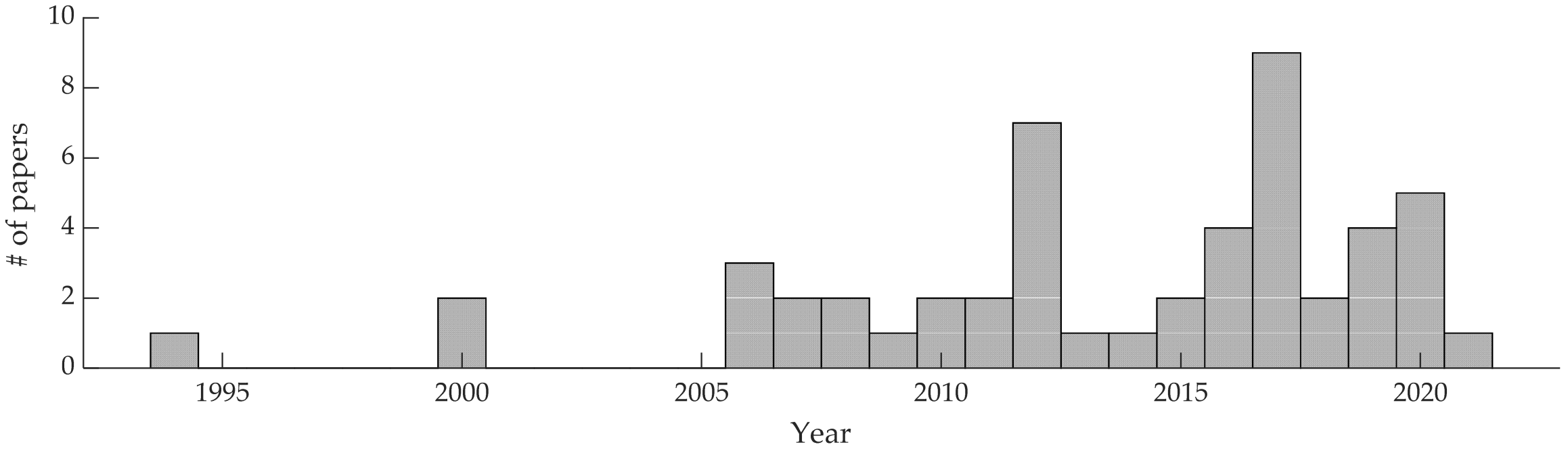
Meshing real-world urban areas for detailed flood modeling may prove very demanding. Indeed, a relatively fine discretization is required to capture relevant flow paths (voids in-between buildings) whose characteristic size is typically a few decameters, while computational domains covering urban areas may extend over hundreds of km2. This makes fast computations particularly challenging [6]. Besides massive parallelization [4,7], another viable option for improving the computational efficiency of urban flood models consists of using subgrid modeling techniques, in which the computation is performed on a relatively coarse grid. At the same time, information on the sub-grid scale topography is preserved [8]. Porosity shallow-water models are a promising sub-grid modeling technique for large-scale urban flood modeling [9,10], as computation times two to three orders of magnitude smaller than standard shallow-water models were reported [11,12,13]. Over the last two decades, rapid advances have been made in the development of porosity shallow-water models (Figure 1).
Therefore, it is deemed timely to conduct a review of the many recent contributions in the field. Half of the studies included in this review were published over the last five years.
Porosity shallow-water models are based on a relatively coarse computational mesh, while so-called porosity parameters are introduced to account for topographic information available at a subgrid-scale [9,10]. This approach is similar to common practice in modeling flow in porous media, such as in groundwater modeling [14].
The presence of an obstacle, such as buildings, in an urban environment, has a threefold effect on the flow: they reduce the volume available for water storage; they channelize the flow along directional pathways defined by the arrangement of the obstacles; and they induce flow resistance due to various mechanisms, such as wakes [15]. The first effect is reproduced using a storage porosity parameter, which indicates the fraction of space available for mass and momentum storage. In all models, this storage porosity is consistently evaluated as the ratio of the volume of void in-between obstacles to the volume of a considered control volume. The other effects are accounted for in various ways, such as by means of additional porosity parameters characterizing the flow conveyance along with specific directions [9,11,15,16,17] or through directional flow resistance terms expressed in the tensor form [18,19].
Many flood models were developed based on the concept of porosity, but they vary greatly in terms of conceptual, mathematical and numerical formulations. As highlighted in Table 1,
Moreover, the underlying flow model may correspond to the complete shallow-water equations (dynamic wave) [9,10,11,12,15,20,22,23] or to an approximation thereof, such as the diffusive wave [24,25,26].
Specific features are included in some models, such as separate flow paths within a single-cell thanks to a multilayered approach [24] or a multiple porosity model [17]. With this review, the authors aim to help the reader navigate through those various formulations of porosity shallow-water models for large-scale urban flood modeling.
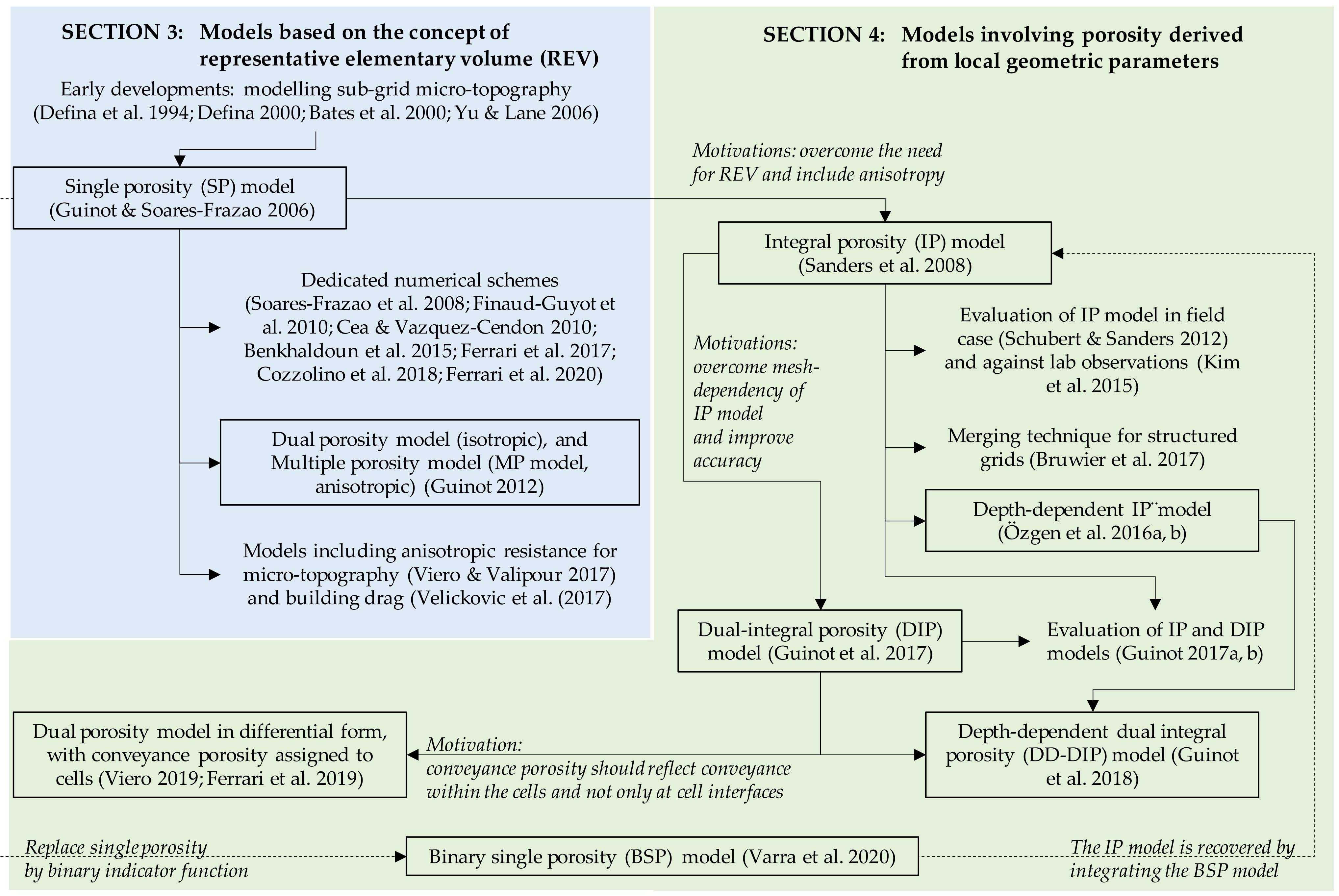
In Section 2, we define the porosity parameters based on a control volume of relevance for urban flood modeling. As suggested by Table 1, there are multiple possibilities for classifying existing porosity shallow-water models. We opted for organizing the review in two-steps. Section 3 presents models in which porosity parameters are defined as statistical descriptors over an area sufficiently large to represent the urban area at a large-scale. In contrast, models that consider porosities defined based on local geometric parameters are detailed in Section 4. Figure 2 provides a schematic representation of the articulation between the major contributions to the field. They are all organized around a handful of landmark papers, as detailed in the following sections. Finally, Section 5 draws attention to recommended directions for future research.
2. Control Volume and Porosity Parameters
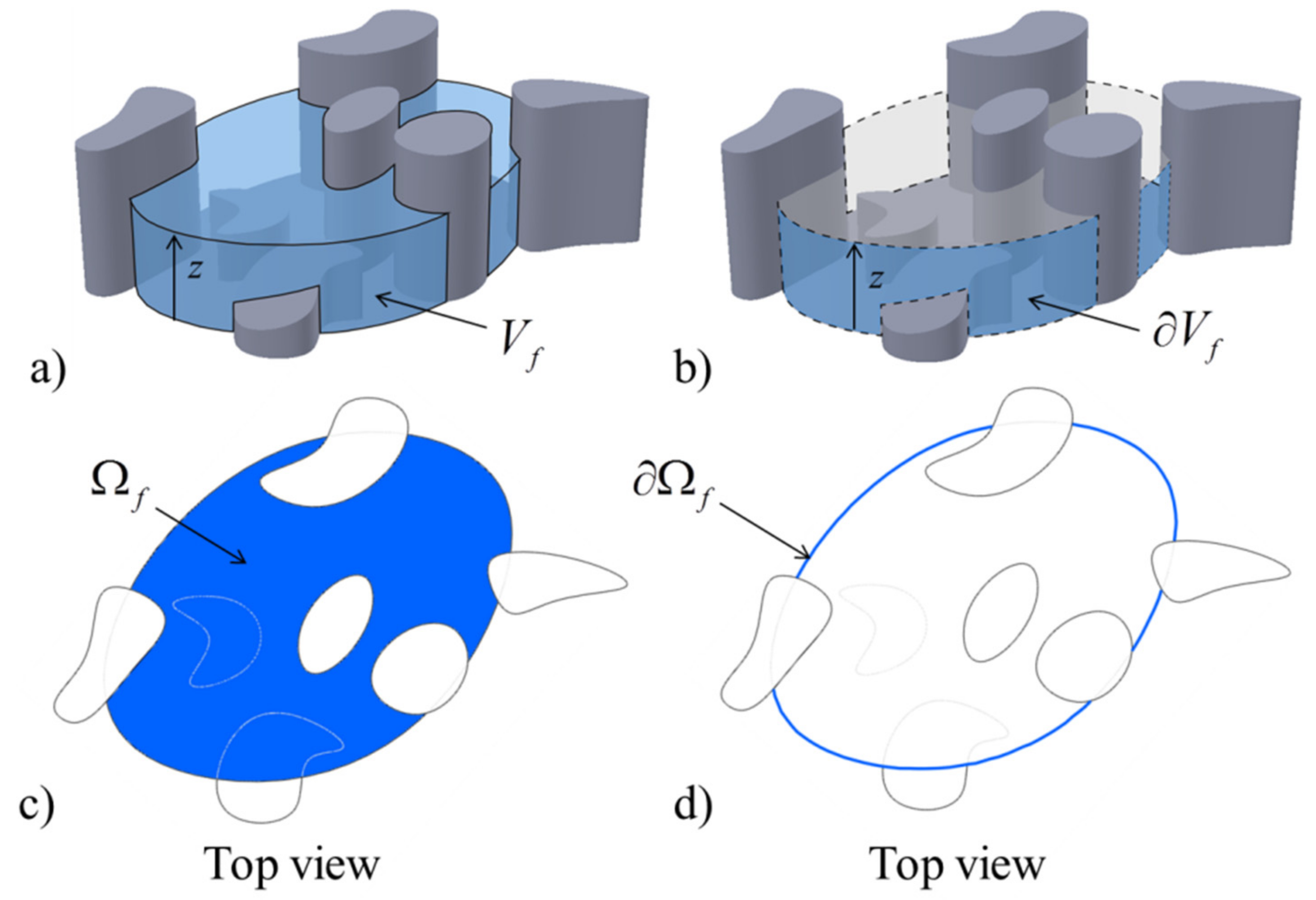
Almost all porosity shallow-water models aim at resolving the flow variables on average over a certain region of space. Hence, in the first place, these models are derived by integrating the flow governing equations over a control volume, as detailed in Appendix A of [10] or in [9]. A control volume of relevance for urban flood modeling is sketched in Figure 3. It is characterized by the presence of rigid obstacles (e.g., buildings) and water in-between. The control volume is delimited downward by the bottom elevation, upward by the water surface and laterally by vertical boundaries. The total volume of the control volume shown in Figure 3 is noted V, while Vf is the part of V filled with water (Figure 3a). Similarly, the contour of V is noted ∂V, while ∂Vf is the part of ∂V through which water can be exchanged (Figure 3b). The projection of the control volume on the horizontal plane x−y is noted Ω, while, for a given arbitrary elevation z, the part Ω corresponding to voids is Ωf (Figure 3c). The contour of Ω is noted ∂Ω, while ∂Ωf is the part of ∂Ω through, which fluid can be exchanged (Figure 3d).
Note that depending on the particular type of porosity shallow-water model, the control volume shown in Figure 3 may correspond to a computational cell [9,11] or to a much wider area (e.g., a representative elementary volume, as discussed in Section 3).
Two types of porosities are used in porosity shallow-water models. First, the storage porosity ϕ, quantifies the volume of voids, i.e., the volume actually available to store water mass and momentum. For a given water level z in a control volume, the storage porosity is expressed mathematically as ϕ(z) = Vf(z)/V(z) [12,22,23]. As highlighted by [23], this definition of ϕ as a function of z is not univocal. It requires an assumption on the shape of the free surface. This shape is often assumed horizontal in the control volume [23].
When the obstacles may be considered prismatic for the range of water depths of interest and that none of them is submerged, the ratio of the volumes Vf and V become independent of the level z. Consequently, the following alternate definition was extensively used when referring to depth-independent storage porosity: ϕ = Ωf/Ω [9,10,11,20].
The conveyance porosity, Ψ, quantifies the fraction of space available for mass and momentum exchange. Unlike the storage porosity, there is not a single clear-cut geometric definition Ψ. Depending on the models, the conveyance porosity is defined either statistically [10,20], or locally at the cell boundary (Ψ(z) = ∂Vf (z)/∂V(z), or Ψ = ∂Ωf/∂Ω in the depth-independent case) [9,11], or at the level of a computational cell (and not just its boundary) [21]. The motivations for these various choices, as well as their implications on model accuracy and mesh sensitivity, are discussed in Section 4.
Note that care must be taken to the nomenclature, as the wording “storage” and “conveyance” porosity was not used uniformly across past studies (Table 2). Particularly, the conveyance porosity is also referred to as connectivity porosity, or areal porosity, among other terms.
3. Models Based on the Concept of Representative Elementary Volume
3.1. Representative Elementary Volume
Pioneering work on porosity shallow-water models was done by Defina et al. (1994) [27] to improve the numerical treatment of wetting and drying fronts when solving the full shallow-water equations. Their approach was later improved by Defina (2000) [28] and Bates (2000) [29]. In these models, the porosity was considered variable with the water depth because it was used as a statistical descriptor of sub-grid microtopographic features and not of buildings. Later, the concept of porosity was transposed to urban flood modeling as a building treatment method [10].
The reasoning underpinning the first porosity shallow-water models consists in idealizing the urban area as a fictitious continuum, in which the flow properties are described by statistical averages at a scale much larger than the scale of individual obstacles and pathways, but also sufficiently small compared to the extent of the whole urban area. This type of approach is widely used for modeling flow in porous media [14], such as in groundwater modeling, and it relies on the concept of representative elementary volume (REV). In general terms, the REV is defined as the smallest control volume for which the statistical properties of the porous medium become independent of the size of this control volume [14]. As pointed out by [17], in the case of a two-dimensional shallow flow model, the REV should normally be called representative elementary area [16], but the terminology REV is preserved here for the sake of consistency with most previous studies [9,17]. We consider these “two-dimensional REVs”.
Provided that it exists in the considered medium, a REV can be defined around any arbitrary point (x,y), irrespective of the positioning of this specific point in water or in an obstacle (Figure 3). Indeed, in all cases, the porosity parameters can be evaluated as averages over the REV, which is much wider than the individual obstacles. It results that, in the REV, the mathematical expectation that a particular point is located in water or in a building is ϕ and 1 − ϕ, respectively.
3.2. Single Porosity Model
By phase-averaging the standard shallow-water equations over a REV containing fluid and obstacles, porosity shallow-water equations were derived by Guinot and Soares-Frazão (2006) [10] (Figure 2). They considered the porosity as depth-independent since it is used to represent the effect of buildings (assumed tall compared to the flow depth) and not of microtopographic features. In general, phase-averaging the shallow-water equations leads to two types of porosity parameters as previously defined: one expressing the available space for mass and momentum storage (ϕ), and the other one referring to the space available for mass and momentum exchange (Ψ). However, the authors of the first models of this type assumed that Ψ = ϕ [10]. This is the reason why this kind of model is called the single-porosity model (SP model).
In a perspective of space-averaging over a REV, a uniform porosity value was generally assigned to the computational cells in the urban area. This choice of a uniform porosity value makes the model unable to reproduce preferential flow directions resulting from directional pathways induced by the arrangement of the buildings at the subgrid-scale. The theoretical wave celerities are identical to those of the standard shallow-water equations [10,11].
The model of Guinot and Soares-Frazao (2006) is expressed in the differential form [10]. Indeed, flow variables (flow depth and depth-averaged velocities) associated with an arbitrary location (x,y) represent an average of the corresponding flow property over a control volume whose centroid is located at the coordinates (x,y). For sufficiently large control volumes (i.e., at minimum equal to the REV), the geometric properties and the flow variables averaged over these control volumes are continuous, differentiable and independent of the specific size chosen for the control volume. A practical advantage of this is that those models do not show an over-sensitivity to the design of the computational mesh. This also relates to the fact that a uniform porosity value was generally assigned to the computational cells in the urban area, no matter how much space is actually occupied by obstacles in each individual cell [18].
Note that, in real-world urban areas, a REV usually does not exist as it would extend beyond the limits of the urban area itself. Nevertheless, based on computational examples, Guinot (2012) [17] highlights that porosity approaches may nonetheless deliver results of practical relevance even for domain sizes smaller than that of the REV. The reason for this is that the errors arising from the porosity evaluation are commensurate with the degree of precision of other parameters or input data in shallow-water models [17].
The resolution of the SP model was performed with several numerical schemes based on the finite volume technique [30,31] and the use of various types of Riemann solvers [10,20,32,33,34,35,36]. Although the SP model was written in differential form, an integral form of the equations was solved numerically since finite volume schemes were used.
3.3. Introducing Anisotropy: Directional Drag, Multiple Porosity Model and Nonuniform Porosity
When the SP model is used with a uniform value of porosity throughout the urban area, a major limitation of such a modeling strategy is its inability to represent directionality [17]. The need for considering two different porosities (storage and conveyance) was pointed out by Lhomme (2006) [37]. However, although two distinct parameters were formally introduced in the governing equations, they were given equal values, and no insight was given on how to infer the value of the conveyance porosity from the geometry of the building footprints [37].
First attempts to introduce anisotropy in the SP model were made through the source term representing buildings drag. Indeed, two types of momentum losses are usually included in the SP model: those due to bottom and sidewall friction, as well as losses induced by the interplay occurring between the flow and the obstructions not explicitly resolved (e.g., wave reflections, building wakes …). In the first implementations of the SP model, the formulation of the corresponding additional sink term was isotropic, and the associated coefficients were taken equal along the x and y directions and evaluated by Borda-like formulations (for the case of a regular grid of buildings) [10,20] or through calibration [35]. In contrast, Velickovic et al. (2017) [18] represented directional effects by introducing a tensor of drag coefficients and amplification coefficients depending on the flow direction. The formulation was later questioned by Guinot (2017) [38], and the use of Borda-like formulae was also invalidated [17]. Similar to [18], a tensor form was used by [19] to model directional flow resistance in the case of overland flow and shallow inundation in agricultural landscapes.
Separately, Guinot (2012) [17] introduced anisotropy in a REV-based model by decomposing the domain into five types of regions: obstacles, regions with stagnant water, regions of isotropic 2D flow, several regions characterized by anisotropic 1D flow and interconnections between the 1D anisotropic flow regions. The immobile regions may be used to represent the wakes of buildings. The different regions exchange mass and momentum as a function of local differences in water levels. Hence, flow exchange coefficients, instead of drag coefficients, need to be calibrated. In each type of region, a specific formulation of the porosity shallow-water equations is used. This approach is called the multiple porosity model (MP model) and is reported to give more accurate results than the SP model [17]. Unlike in the SP model, the MP model’s theoretical wave celerities differ from those in the standard shallow-water equations. The MP model of Guinot (2012) [17] may be reduced to an isotropic dual-porosity formulation if only obstacles, stagnant water and 2D isotropic flow regions are considered.
While most studies based on the SP model used a uniform value of porosity in the whole urban area, several authors [39,40,41] demonstrated the viability of finite volume schemes for the solution of SP models with a local storage porosity defined at the level of computational cells, regardless of the conceptual problems linked to the REV definition. Considering a porosity value variable from one cell to another in the SP model enables reproducing preferential flow paths and hence anisotropy. These models can be regarded as particular applications of the binary single porosity model recently proposed by Varra et al. (2020) [42] and described in Section 4.4.
4. Models Involving Porosity Derived from Local Geometric Parameters
4.1. Integral Porosity Model
Another line of research was also followed for the development of porosity shallow-water models. Along this line, the concept of REV is not used, and the equations are written in integral form for a control volume, which is either taken equal to a computational cell [9] or arbitrary (i.e., irrespective of a particular discretization) [11,23]. The main motivation for this approach was to overcome the theoretical limitation related to the inexistence of a REV in most real-world urban areas, as well as the inability of the SP model to reproduce directional effects.
In a landmark paper, Sanders et al. (2008) [9] used the Reynolds transport theorem and a binary density function to derive a macroscopic form of mass conservation and momentum equations, called the integral porosity model (IP model). In these equations, written in integral form, both storage and conveyance porosities are involved. The storage porosity ϕ is computed similarly as in the SP model but considering one computational cell instead of the REV as control volume. The conveyance porosity Ψ is defined as the fraction of a boundary of a computational cell, which contributes to mass and momentum exchange. Sanders et al. (2008) [9] indicate how to compute this parameter from geospatial data, such as classified aerial imagery or a digital elevation model and vector data describing building footprints.
Although the IP model was originally written in integral form, deriving a differential analog is useful for checking numerical convergence and for evaluating the wave celerities [17]. In a first attempt to do so, several authors estimated that the theoretical wave celerities of the IP model differ from those of the standard shallow-water equations [11,37,39]. In particular, they concluded that the conveyance porosity Ψ, which accounts for building obstruction to the flow, must be smaller than the storage porosity ϕ; otherwise, wave celerities larger than in the case without obstruction would be obtained, which appears unphysical [11,38]. Nonetheless, this constraint was recently questioned by Varra et al. (2020) [42], who proposed another differential equivalent of the IP model, as detailed in Section 4.4. According to [42], the differential analogs considered earlier cannot be used to evaluate wave celerities of the IP model.
Unlike the single porosity in the SP model, both the storage and the conveyance porosities introduced by [9] are defined locally at the level of computational cells or cell boundaries. Additionally, the conveyance porosity of [9] depends on the orientation of the cell boundary, which enables anisotropy of the urban area to be accounted for. These features make the model of [9] more accurate [13,39] and more suitable than the SP model for reproducing directional effects induced by obstructions not explicitly resolved in the computations, but it also makes this model overly sensitive to the mesh design [17,43]. Guidelines were formulated and assessed for designing suitable meshes.
A so-called gap-conforming mesh is recommended [9] to capture the anisotropy of urban networks through the conveyance porosity parameters by ensuring that computational edges intersect the obstacles indeed. However, these guidelines for mesh design do not completely fix the mesh over-sensitivity of the IP model and are not applicable to all types of meshes (e.g., Cartesian) [6,9,43]. A technique consisting of merging computational cells with low porosity values was proposed by [44] for the case of Cartesian grids.
To account for head losses induced by subgrid-scale buildings, the IP model uses a quadratic drag expression in the model equations [9]. It involves a drag coefficient and the projected area of the obstructions as seen by an observer moving along the flow direction. In general, these quantities are both direction- and flow-dependent, but a single scalar value was used by [9]. Determining these values for real-world applications is not straightforward. For the case of a field test with complex building geometry and topographic variations, a simplified version of the building drag term was tested by [6]: the flow-direction dependence of the frontal area of obstructions was ignored, and this quantity was computed as the average of the frontal area of obstructions over the directions of all cell boundaries.
Özgen et al. (2016) [12,22] proposed an extension of the IP model, in which the storage and conveyance porosities are depth-dependent. Approaches similar to that of Sanders et al. (2008) [9] and Özgen et al. (2016) [12] were adopted in multiple other studies, which account for obstruction-induced effects on storage and conveyance at the level of each computational cell [4,8,24,25,26,45,46,47,48,49,50,51]. Various approximations of the shallow-water equations were used in these studies (e.g., diffusive wave), and the storage and conveyance properties were generally considered as depth-dependent. For pluvial flooding applications, Chen et al. (2012) [25] derived an integral porosity model based on a diffusive wave approximation. No building drag term was considered. Representing separate flow paths within a single-cell of a Cartesian grid was made possible in an upgraded version of the same model [24]. This feature is based on a multilayered approach, and it shows similarity with the MP model [17].
4.2. Dual Integral Porosity Model
In another landmark paper, Guinot et al. (2017) [11] derived the dual integral porosity model (DIP model) considering an arbitrary control volume (not necessarily linked to a computational cell). The DIP model is an extension of the IP model, which aims at correcting discrepancies between wave celerities obtained from the IP model and from refined calculations based on the standard shallow-water equations. Compared to the IP model, the DIP model contains three major conceptual improvements: (i) porosity and flow variables are defined separately for control volumes and boundaries, and a closure scheme is proposed to link control volume-based and boundary-based quantities; (ii) a new transient momentum dissipation mechanism active for positive waves is introduced, and (iii) an anisotropic drag force model is formulated.
As shown by [17], when a positive wave propagates in an urban area, wave reflections occur against the buildings and generate moving bores. The forces exerted by the building walls are opposed to the average flow velocity and thus contribute to dissipating momentum. Similar bores do not occur in the case of steady flow nor for decreasing water levels [17]. This momentum dissipation mechanism cannot be described by an equation of state, i.e., involving only the flow variables. Hence, it cannot be reproduced by means of a building drag term [23]. Therefore, Guinot et al. (2017) [11] introduced this dissipation mechanism directly in the fluxes of the model by means of a tensor whose elements need to be calibrated. It is active only under transient conditions involving positive waves (rising water levels).
Note that the closure scheme proposed by Guinot et al. (2017) [11] leads to using only the storage porosity in the continuity fluxes. This contrasts with the original IP model, but it makes the new continuity equation consistent with that originally derived by Defina [28]. For the DIP model to be well-posed, it is necessary that the conveyance porosity is lower than the storage porosity, as mentioned above for the IP model [38].
Based on a set of 96 benchmarks, enabling direct validation of flux closures and source terms, the DIP model was shown to outperform the IP and SP models [38]. The DIP model was also shown to be substantially less sensitive to mesh design than the IP model [43]. Similar to the extension brought by [12] to the IP model, Guinot et al. (2018) [23] proposed a new formulation of the DIP model, in which the porosities are depth-dependent, and the model is adapted to handle submerged obstructions. In this study, the superiority of the DIP model over the IP model is confirmed, and the transient momentum dissipation mechanism is shown to be essential [23].
4.3. Alternate Uses and Definitions of Conveyance Porosities
To further reduce the model sensitivity to the design of the mesh, Viero (2019) [16] implemented a dual-porosity model, in which the conveyance porosity is not evaluated locally at the cell interfaces but at the level of each computational cell, and it is defined along mutually orthogonal principal directions. It is assumed that water flows through the narrowest cross-section over the computational cell, as already assumed by [44] among others. This is justified by the occurrence of most dissipation at locations where velocity is the largest and by the fact that the effective length of the narrowest section is longer than its geometric length due to the jet developing downstream of a contraction [16]. Unlike previous implementations of the IP and DIP models using collocated finite volume schemes, a finite element scheme was used on a staggering unstructured mesh [16]. Tests against refined numerical solutions and experimental data suggest that the model sensitivity to the mesh design is acceptable in the tested configurations.
With the same objective of further reducing model mesh sensitivity, Ferrari et al. (2019) [15] considered an isotropic single porosity formulation for the fluxes and used anisotropic conveyance porosities to estimate flow resistance by means of a directionally dependent tensor formulation. Like in [16], the effective velocity for evaluating losses is determined from the narrowest cross-section in the considered urban district. The authors conclude that the model is not oversensitive to mesh resolution and design, but they call for more research on the determination of the conveyance porosity for real-world urban areas. This issue has been addressed by Ferrari and Viero (2020) [21], who detail an algorithm for computing distributed cell-based conveyance porosities as needed in the dual-porosity models. It is based on the analysis of the footprints of buildings and obstacles on Cartesian grids and uses mutually orthogonal principal directions. This approach performs well in the presence of a single dominant obstacle in the cell but not with multiple obstacles. Therefore, more research is needed regarding the modeling of conveyance porosity.
4.4. Binary Single Porosity Model
In a recent theoretical contribution, Varra et al. (2020) [42] introduced the binary single porosity model (BSP model), a novel local, differential porosity model formulation derived regardless of the existence of a REV. The BSP model adopts the same mathematical formulation as the SP model, the REV-based porosity parameter of the SP model being replaced by a binary indicator (equal to unity in the water and to zero in the obstacles). Therefore, derivatives in the BSP differential form must be understood in the sense of generalized functions (distributions). The IP model may be recovered from the BSP model by integration in space. As the derivation of the BSP model does not involve space averaging, the flow variables are pointwise and not space averaged values.
Varra et al. (2020) [42] claim that a suitable Riemann solver has the potential to take into account energy loss due to wave reflections, hence reducing the need to resort to additional drag terms. In addition, additional stationary dissipation is needed through porosity reductions in supercritical flow.
Despite encouraging results obtained so far with the dual porosity models [11,16,23,38,43], Varra et al. (2020) [42] indicates that the use of different storage and conveyance porosities in the mathematical model formulation in differential form violates the Galilean invariance and that the difference between storage and conveyance porosities arises in the numerical discretization, but should not be introduced in the model mathematical formulation. This further emphasizes the need for additional research on the modeling of anisotropic conveyance effects in porosity shallow-water models.
5. Directions for Further Research
This paper reviews the various porosity shallow-water models developed so far for large-scale urban flood modeling. Two main families of porosity models can be distinguished depending on the scale at which porosity parameters are determined (REV-based porosity vs. porosity derived from local geometric data). Recent developments have been numerous. They have addressed multiple aspects of the models, such as more physically grounded modeling of momentum dissipation mechanisms, enhanced determination of conveyance porosities, strategies to mitigate mesh over-sensitivity of integral porosity models or new insights into the theoretical formulation of the models.
Despite many efforts devoted to the formulation of models for building drag and other dissipation mechanisms, none of the current models is complete [38]. There are still gaps in knowledge regarding not only the calibration but also the structure of dissipation mechanism models adapted to porosity shallow-water equations for large-scale urban flood modeling. This calls for more research on both the conceptual and numerical aspects [42].
Recent advances in porosity models were not all evaluated based on the same test cases. This may influence conclusions drawn on the model’s performance, such as accuracy or degree of mesh sensitivity. The scientific community would highly benefit from the setup of a series of accepted benchmarks against which every new contribution could be assessed. This would take the form of an evolving, shared database of test cases as it does exist in other fields. Such test cases should incorporate a blend of idealized, synthetic [52] and fully realistic configurations, including high-quality field observations of flow depth and velocity. Particularly valuable are direct evaluations of flux and source terms [38], as well as disentangling structural, scaling and porosity model errors [13].
The transfer of porosity shallow-water models from research to practice poses specific challenges [4]. Guidelines should be developed to enable practitioners to achieve optimal mesh design and model calibration. However, a general methodology for model parametrization for real-world urban areas remains a research question. Strategies could be elaborated for calibrating porosity models using fine-scale reference model runs over only a limited domain or for optimally combining porosity and detailed models using domain decomposition or nested models.
Flow modeling results are often used as input for complementary analyses, such as damage modeling, solute [46] or sediment transport and morphodynamic modeling. It is, therefore, necessary to assess whether the porosity models succeed in predicting, at the right scale, the flow variables needed for these complementary analyses and which postprocessing steps may be necessary [53].
Author Contributions
Conceptualization, B.D., P.A. and M.B.; formal analysis, B.D. and M.B.; writing—original draft, B.D. and M.B.; writing—review and editing, B.D., P.A., S.E., M.P. All authors have read and agreed to the published version of the manuscript.
Funding
This research received no external funding.
Informed Consent Statement
Not applicable.
Acknowledgments
The authors gratefully acknowledge two anonymous reviewers whose insightful comments substantially improved several aspects of the manuscript.
Conflicts of Interest
The authors declare no conflict of interest.
References
- Ward, P.J.; Blauhut, V.; Bloemendaal, N.; Daniell, E.J.; De Ruiter, C.M.; Duncan, J.M.; Emberson, R.; Jenkins, F.S.; Kirschbaum, D.; Kunz, M.; et al. Review article: Natural hazard risk assessments at the global scale. Nat. Hazards Earth Syst. Sci. 2020, 20, 1069–1096. [Google Scholar] [CrossRef] [Green Version]
- Aerts, J.C.J.H.; Botzen, W.J.W.; Emanuel, K.; Lin, N.; De Moel, H.; Michel-Kerjan, E.O. Climate adaptation: Evaluating flood resilience strategies for coastal megacities. Science 2014, 344, 473–475. [Google Scholar] [CrossRef]
- IPCC. Managing the Risks of Extreme Events and Disasters to Advance Climate Change Adaptation—A Special Report of Working Groups I and II of the IPCC; Field, C.B., Barros, V., Stocker, T.F., Qin, D., Dokken, D.J., Ebi, K.L., Mastrandrea, M.D., Mach, K.J., Plattner, G.-K., Allen, S.K., et al., Eds.; Cambridge University Press: Cambridge, UK, 2012. [Google Scholar]
- Sanders, B.F.; Schubert, J.E. PRIMo: Parallel raster inundation model. Adv. Water Resour. 2019, 126, 79–95. [Google Scholar] [CrossRef]
- Dottori, F.; Di Baldassarre, G.; Todini, E. Detailed data is welcome, but with a pinch of salt: Accuracy, precision, and uncertainty in flood inundation modeling. Water Resour. Res. 2013, 49, 6079–6085. [Google Scholar] [CrossRef]
- Schubert, J.E.; Sanders, B.F. Building treatments for urban flood inundation models and implications for predictive skill and modeling efficiency. Adv. Water Resour. 2012, 41, 49–64. [Google Scholar] [CrossRef]
- Yu, D. Parallelization of a two-dimensional flood inundation model based on domain decomposition. Environ. Model. Softw. 2010, 25, 935–945. [Google Scholar] [CrossRef] [Green Version]
- McMillan, H.K.; Brasington, J. Reduced complexity strategies for modelling urban floodplain inundation. Geomorphology 2007, 90, 226–243. [Google Scholar] [CrossRef]
- Sanders, B.F.; Schubert, J.E.; Gallegos, H.A. Integral formulation of shallow-water equations with anisotropic porosity for urban flood modeling. J. Hydrol. 2008, 362, 19–38. [Google Scholar] [CrossRef]
- Guinot, V.; Soares-Frazão, S. Flux and source term discretization in two-dimensional shallow water models with porosity on unstructured grids. Int. J. Numer. Methods Fluids 2006, 50, 309–345. [Google Scholar] [CrossRef]
- Guinot, V.; Sanders, B.F.; Schubert, J.E. Dual integral porosity shallow water model for urban flood modelling. Adv. Water Resour. 2017, 103, 16–31. [Google Scholar] [CrossRef] [Green Version]
- Özgen, I.; Liang, D.; Hinkelmann, R. Shallow water equations with depth-dependent anisotropic porosity for subgrid-scale topography. Appl. Math. Model. 2016, 40, 7447–7473. [Google Scholar] [CrossRef] [Green Version]
- Kim, B.; Sanders, B.F.; Famiglietti, J.S.; Guinot, V. Urban flood modeling with porous shallow-water equations: A case study of model errors in the presence of anisotropic porosity. J. Hydrol. 2015, 523, 680–692. [Google Scholar] [CrossRef] [Green Version]
- Bear, J. Dynamics of Fluids in Porous Media; Dover Publications Inc.: New York, NY, USA, 1988. [Google Scholar]
- Ferrari, A.; Viero, D.P.; Vacondio, R.; Defina, A.; Mignosa, P. Flood inundation modeling in urbanized areas: A mesh-independent porosity approach with anisotropic friction. Adv. Water Resour. 2019, 125, 98–113. [Google Scholar] [CrossRef]
- Viero, D.P. Modelling urban floods using a finite element staggered scheme with an anisotropic dual porosity model. J. Hydrol. 2019, 568, 247–259. [Google Scholar] [CrossRef] [Green Version]
- Guinot, V. Multiple porosity shallow water models for macroscopic modelling of urban floods. Adv. Water Resour. 2012, 37, 40–72. [Google Scholar] [CrossRef]
- Velickovic, M.; Zech, Y.; Soares-Frazão, S. Steady-flow experiments in urban areas and anisotropic porosity model. J. Hydraul. Res. 2017, 55, 85–100. [Google Scholar] [CrossRef]
- Viero, D.P.; Valipour, M. Modeling anisotropy in free-surface overland and shallow inundation flows. Adv. Water Resour. 2017, 104, 1–14. [Google Scholar] [CrossRef]
- Soares-Frazão, S.; Lhomme, J.; Guinot, V.; Zech, Y. Two-dimensional shallow-water model with porosity for urban flood modelling. J. Hydraul. Res. 2008, 46, 45–64. [Google Scholar] [CrossRef]
- Ferrari, A.; Viero, D.P. Floodwater pathways in urban areas: A method to compute porosity fields for anisotropic subgrid models in differential form. J. Hydrol. 2020, 589. [Google Scholar] [CrossRef]
- Özgen, I.; Zhao, J.; Liang, D.; Hinkelmann, R. Urban flood modeling using shallow water equations with depth-dependent anisotropic porosity. J. Hydrol. 2016, 541, 1165–1184. [Google Scholar] [CrossRef] [Green Version]
- Guinot, V.; Delenne, C.; Rousseau, A.; Boutron, O. Flux closures and source term models for shallow water models with depth-dependent integral porosity. Adv. Water Resour. 2018, 122, 1–26. [Google Scholar] [CrossRef] [Green Version]
- Chen, A.S.; Evans, B.; Djordjević, S.; Savić, D.A. Multi-layered coarse grid modelling in 2D urban flood simulations. J. Hydrol. 2012, 470–471, 1–11. [Google Scholar] [CrossRef] [Green Version]
- Chen, A.S.; Evans, B.; Djordjević, S.; Savić, D.A. A coarse-grid approach to representing building blockage effects in 2D urban flood modelling. J. Hydrol. 2012, 426–427, 1–16. [Google Scholar] [CrossRef] [Green Version]
- Yu, D.; Lane, S.N. Urban fluvial flood modelling using a two-dimensional diffusion-wave treatment, part 2: Development of a sub-grid-scale treatment. Hydrol. Process. 2006, 20, 1567–1583. [Google Scholar] [CrossRef]
- Defina, A.; D’Alpaos, L.; Matticchio, B. New set of equations for very shallow water and partially dry areas suitable to 2D numerical models. In Proceedings of the Specialty Conference on Modelling of Flood Propagation Over Initially Dry Areas, Milan, Italy, 29 June–1 July 1994; ASCE: Reston, VA, USA, 1994; pp. 72–81. [Google Scholar]
- Defina, A. Two-dimensional shallow flow equations for partially dry areas. Water Resour. Res. 2000, 36, 3251–3264. [Google Scholar] [CrossRef] [Green Version]
- Bates, P.D. Development and testing of a subgrid-scale model for moving-boundary hydrodynamic problems in shallow water. Hydrol. Process. 2000, 14, 2073–2088. [Google Scholar] [CrossRef]
- Cozzolino, L.; Pepe, V.; Cimorelli, L.; D’Aniello, A.; Della Morte, R.; Pianese, D. The solution of the dam-break problem in the porous shallow water equations. Adv. Water Resour. 2018, 114, 83–101. [Google Scholar] [CrossRef]
- Mohamed, K. A finite volume method for numerical simulation of shallow water models with porosity. Comput. Fluids 2014, 104, 9–19. [Google Scholar] [CrossRef]
- Ferrari, A.; Vacondio, R.; Mignosa, P. A second-order numerical scheme for the porous shallow water equations based on a DOT ADER augmented Riemann solver. Adv. Water Resour. 2020, 140. [Google Scholar] [CrossRef]
- Ferrari, A.; Vacondio, R.; Dazzi, S.; Mignosa, P. A 1D–2D shallow water equations solver for discontinuous porosity field based on a generalized Riemann problem. Adv. Water Resour. 2017, 107, 233–249. [Google Scholar] [CrossRef]
- Benkhaldoun, F.; Elmahi, I.; Moumna, A.; Seaid, M. A non-homogeneous Riemann solver for shallow water equations in porous media. Appl. Anal. 2016, 95, 2181–2202. [Google Scholar] [CrossRef] [Green Version]
- Cea, L.; Vázquez-Cendón, M.E. Unstructured finite volume discretization of two-dimensional depth-averaged shallow water equations with porosity. Int. J. Numer. Methods Fluids 2010, 63, 903–930. [Google Scholar] [CrossRef]
- Finaud-Guyot, P.; Delenne, C.; Lhomme, J.; Guinot, V.; Llovel, C. An approximate-state Riemann solver for the two-dimensional shallow water equations with porosity. Int. J. Numer. Methods Fluids 2010, 62, 1299–1331. [Google Scholar] [CrossRef]
- Lhomme, J. One-Dimensional, Two-Dimensional and Macroscopic Approaches to Urban Flood Modelling. Ph.D.Thesis, Montpellier 2 University, Montpellier, France, 2006. [Google Scholar]
- Guinot, V. A critical assessment of flux and source term closures in shallow water models with porosity for urban flood simulations. Adv. Water Resour. 2017, 109, 133–157. [Google Scholar] [CrossRef] [Green Version]
- Özgen, I.; Zhao, J.-H.; Liang, D.-F.; Hinkelmann, R. Wave propagation speeds and source term influences in single and integral porosity shallow water equations. Water Sci. Eng. 2017, 10, 275–286. [Google Scholar] [CrossRef]
- Velickovic, M.; Van Emelen, S.; Zech, Y.; Soares-Frazão, S. Shallow-water model with porosity: Sensitivity analysis to head losses and porosity distribution. In Proceedings of the River flow 2010: International Conference on Fluvial Hydraulics, Braunschweig, Germany, 8–10 September 2010; Dittrich, A., Koll, K., Aberle, J., Geisenhainer, P., Eds.; Bundesanstalt für Wasserbau: Karlsruhe, Germany, 2010; Volume 2, pp. 613–620. [Google Scholar]
- Soares-Frazão, S.; Franzini, F.; Linkens, J.; Snaps, J.-C. Investigation of distributed-porosity fields for urban flood modelling using single-porosity models. In Proceedings of the E3S Web of Conferences, Lyon, France, 6–8 April 2018; Volume 40, p. 06040. [Google Scholar]
- Varra, G.; Pepe, V.; Cimorelli, L.; Della Morte, R.; Cozzolino, L. On integral and differential porosity models for urban flooding simulation. Adv. Water Resour. 2020, 136. [Google Scholar] [CrossRef]
- Guinot, V. Consistency and bicharacteristic analysis of integral porosity shallow water models. Explaining model oversensitivity to mesh design. Adv. Water Resour. 2017, 107, 43–55. [Google Scholar] [CrossRef] [Green Version]
- Bruwier, M.; Archambeau, P.; Erpicum, S.; Pirotton, M.; Dewals, B. Shallow-water models with anisotropic porosity and merging for flood modelling on Cartesian grids. J. Hydrol. 2017, 554, 693–709. [Google Scholar] [CrossRef]
- Li, Z.; Hodges, B.R. On modeling subgrid-scale macro-structures in narrow twisted channels. Adv. Water Resour. 2020, 135. [Google Scholar] [CrossRef]
- Li, Z.; Hodges, B.R. Modeling subgrid-scale topographic effects on shallow marsh hydrodynamics and salinity transport. Adv. Water Resour. 2019, 129, 1–15. [Google Scholar] [CrossRef]
- Shamkhalchian, A.; De Almeida, G.A.M. Upscaling the shallow water equations for fast flood modelling. J. Hydraul. Res. 2020. [Google Scholar] [CrossRef]
- Wu, G.; Shi, F.; Kirby, J.T.; Mieras, R.; Liang, B.; Li, H.; Shi, J. A pre-storage, subgrid model for simulating flooding and draining processes in salt marshes. Coast. Eng. 2016, 108, 65–78. [Google Scholar] [CrossRef]
- Volp, N.D.; Van Prooijen, B.C.; Stelling, G.S. A finite volume approach for shallow water flow accounting for high-resolution bathymetry and roughness data. Water Resour. Res. 2013, 49, 4126–4135. [Google Scholar] [CrossRef] [Green Version]
- Neal, J.; Schumann, G.; Bates, P. A subgrid channel model for simulating river hydraulics and floodplain inundation over large and data sparse areas. Water Resour. Res. 2012, 48, W11506. [Google Scholar] [CrossRef]
- Casulli, V.; Stelling, G.S. Semi-implicit subgrid modelling of three-dimensional free-surface flows. Int. J. Numer. Methods Fluids 2011, 67, 441–449. [Google Scholar] [CrossRef]
- Bruwier, M.; Mustafa, A.; Aliaga, D.G.; Archambeau, P.; Erpicum, S.; Nishida, G.; Zhang, X.; Pirotton, M.; Teller, J.; Dewals, B. Influence of urban pattern on inundation flow in floodplains oflowland rivers. Sci. Total Environ. 2018, 622–623, 446–458. [Google Scholar] [CrossRef] [Green Version]
- Carreau, J.; Guinot, V. A PCA spatial pattern based artificial neural network downscaling model for urban flood hazard assessment. Adv. Water Resour. 2021, 147. [Google Scholar] [CrossRef]
Figure 1.
Number of papers included in this review as a function of the publication year.

Figure 2.
Articulation between selected major contributions to the development of porosity shallow-water models for large-scale urban flood modeling.
Figure 2.
Articulation between selected major contributions to the development of porosity shallow-water models for large-scale urban flood modeling.

Figure 3.
Sketch of a control volume and (a) the part Vf occupied by water, (b) the fluid–fluid exchange boundary ∂Vf, (c) a horizontal surface at a given level z and its part occupied by water Ωf, as well as (d) the fluid–fluid exchange border ∂Ωf of the horizontal surface.
Figure 3.
Sketch of a control volume and (a) the part Vf occupied by water, (b) the fluid–fluid exchange boundary ∂Vf, (c) a horizontal surface at a given level z and its part occupied by water Ωf, as well as (d) the fluid–fluid exchange border ∂Ωf of the horizontal surface.


Table 1.
Dualities in existing porosity models.
| Porosity as a Atatistical Descriptor [10,20] | Porosity as a Deterministic Geometric Parameter [9,11,21] |
|---|---|
| Single porosity parameter [10,20] (e.g., conveyance porosity equal to storage porosity) | Multiple porosity parameters [9,11,15,16,17] |
| Isotropic porosity effects [10,20] | Anisotropic porosity effects [9,11,12,15,16,21,22,23] |
| Depth-independent porosity [9,10,11,17] | Depth-dependent porosity [12,22,23] |
| Model expressed in differential form [10,20,21] | Model expressed in the integral form [9,11] |
| Numerical scheme limited to subcritical flow [16] | Shock-capturing schemes [9,10,11,12,15,20,22,23] |
| Shallow-water (dynamic wave) [9,10,11,12,15,20,22,23] | Diffusive wave approximation [24,25,26] |
| Isotropic flow resistance, e.g., [6] | Directional flow resistance [18,19] |
Table 2.
Nomenclature used in existing research to denote storage and conveyance porosities.
| Context | References | Parameter Reflecting Storage Capacity in Control Volumes | Parameter Reflecting Fraction of Space Available for Flow Conveyance |
|---|---|---|---|
| Depth-independent porosity model | [1,2,6,7,8] | Storage porosity | Conveyance porosity |
| [9,10,11] | Storage (or areal) porosity | Connectivity (or frontal) porosity | |
| [12,13] | 1 − BCR, with BCR = building coverage ratio | 1 − CRF, with CRF = conveyance reduction factors | |
| [5,15] | Volumetric porosity | Areal porosity | |
| Depth-dependent porosity model | [16,17,20,21] |
Publisher’s Note: MDPI stays neutral with regard to jurisdictional claims in published maps and institutional affiliations. |
© 2021 by the authors. Licensee MDPI, Basel, Switzerland. This article is an open access article distributed under the terms and conditions of the Creative Commons Attribution (CC BY) license (https://creativecommons.org/licenses/by/4.0/).
Share and Cite
MDPI and ACS Style
Dewals, B.; Bruwier, M.; Pirotton, M.; Erpicum, S.; Archambeau, P. Porosity Models for Large-Scale Urban Flood Modelling: A Review. Water 2021, 13, 960. https://doi.org/10.3390/w13070960
AMA Style
Dewals B, Bruwier M, Pirotton M, Erpicum S, Archambeau P. Porosity Models for Large-Scale Urban Flood Modelling: A Review. Water. 2021; 13(7):960. https://doi.org/10.3390/w13070960
Chicago/Turabian StyleDewals, Benjamin, Martin Bruwier, Michel Pirotton, Sebastien Erpicum, and Pierre Archambeau. 2021. "Porosity Models for Large-Scale Urban Flood Modelling: A Review" Water 13, no. 7: 960. https://doi.org/10.3390/w13070960
Note that from the first issue of 2016, this journal uses article numbers instead of page numbers. See further details here.