
Modeling Nickel Leaching from Abandoned Mine Tailing Deposits in Jøssingfjorden


1
Norwegian Institute for Water Research (NIVA), Gaustadalléen 21, 0349 Oslo, Norway
2
P.P.Shirshov Institute of Oceanology RAS, Nakhimovskiy prosp. 36, 117991 Moscow, Russia
*
Author to whom correspondence should be addressed.
Water 2021, 13(7), 967; https://doi.org/10.3390/w13070967
Submission received: 1 February 2021
/
Revised: 12 March 2021
/
Accepted: 20 March 2021
/
Published: 31 March 2021
(This article belongs to the Special Issue Marine Biogeochemical Modeling)
Abstract
:Underwater disposal of mine tailings in lakes and seas has been considered favorable due to the geochemical stability obtained during long-term storage in anoxic sediments. Sulfides are stable in the ore; however, oxidation and transformation of some substances into more soluble forms may impact bioavailability processes and enhance the risk of toxic effects in the aquatic environment. The goal of this work was to construct a model for simulating the nickel (Ni) cycle in the water column and upper sediments and apply it to the mine tailing sea deposit in the Jøssingfjord, SouthWest Norway. A one-dimensional (1D) benthic–pelagic coupled biogeochemical model, BROM, supplemented with a Ni module specifically developed for the study was used. The model was optimized using field data collected from the fjord. The model predicted that the current high Ni concentrations in the sediment can be a potential source of Ni leaching to the water column until about 2040. The top 10 cm of sediments were classified as being of “poor” environmental state according to the Norwegian Quality Standards. A numerical experiment predicted that with complete cessation of the discharges there would be an improvement in the environmental state of sediment to “good” in about 20 years. On the other hand, doubling of discharge would lead to an increase in the Ni content in the sediment, approaching the boundary of the “very poor” environmental state. The model results demonstrated that Ni leaching from the sea deposits may be increased due to sediment reworking by bioturbation at the sediment–water interface. The model can be an instrument for analysis of different scenarios for mine tailing activities from point of view of reduction of environmental impact as a component of the best available technology.
1. Introduction
Tailings from the mining industry are fine-grained rock materials left over from the process of separating the valuable fraction from the uneconomic fraction of an ore. In addition to fragmented rock material, tailings may contain potentially harmful substances such as trace metals and remnants of production chemicals [1]. Even the particles themselves may have detrimental effects on living organisms related to hypersedimentation and altered size and shape which may disturb vital habitat and physiological functions of some species [2].
The global mineral production in 2012 was 16 billion tons per year [3]. The production, along with the problem of waste disposal, is rising exponentially with increasing demand for metals and other mineral products [4].
Underwater disposal in lakes and seas has been considered favorable due to the geochemical stability obtained during long-term storage in anoxic sediments [5,6,7]. Some ores contain sulfide minerals. Metal sulfides are stable in the ore, but bioavailability and risk of toxic effects may increase in the water environment due to oxidation and transformation into more soluble forms [8]. Therefore, the leaching of metals such as Cu, Ni, Co, As, Cd, Zn, Pb, and Hg is a major issue in the disposal of tailings and mineral products from these mines [7,9,10,11]. Leaching of trace metals from waste rocks and tailings has been reported to be a source of trace metal input for many decades after the cessation of mining activities. Oxidation and dissolution may be prolonged in lake or sea deposits due to sediment reworking by bioturbation at the sediment–water interface [12,13,14].
In Norway and other coastal countries, sea deposits are convenient due to the availability of sea areas near the mineral ore locations [2,15,16].
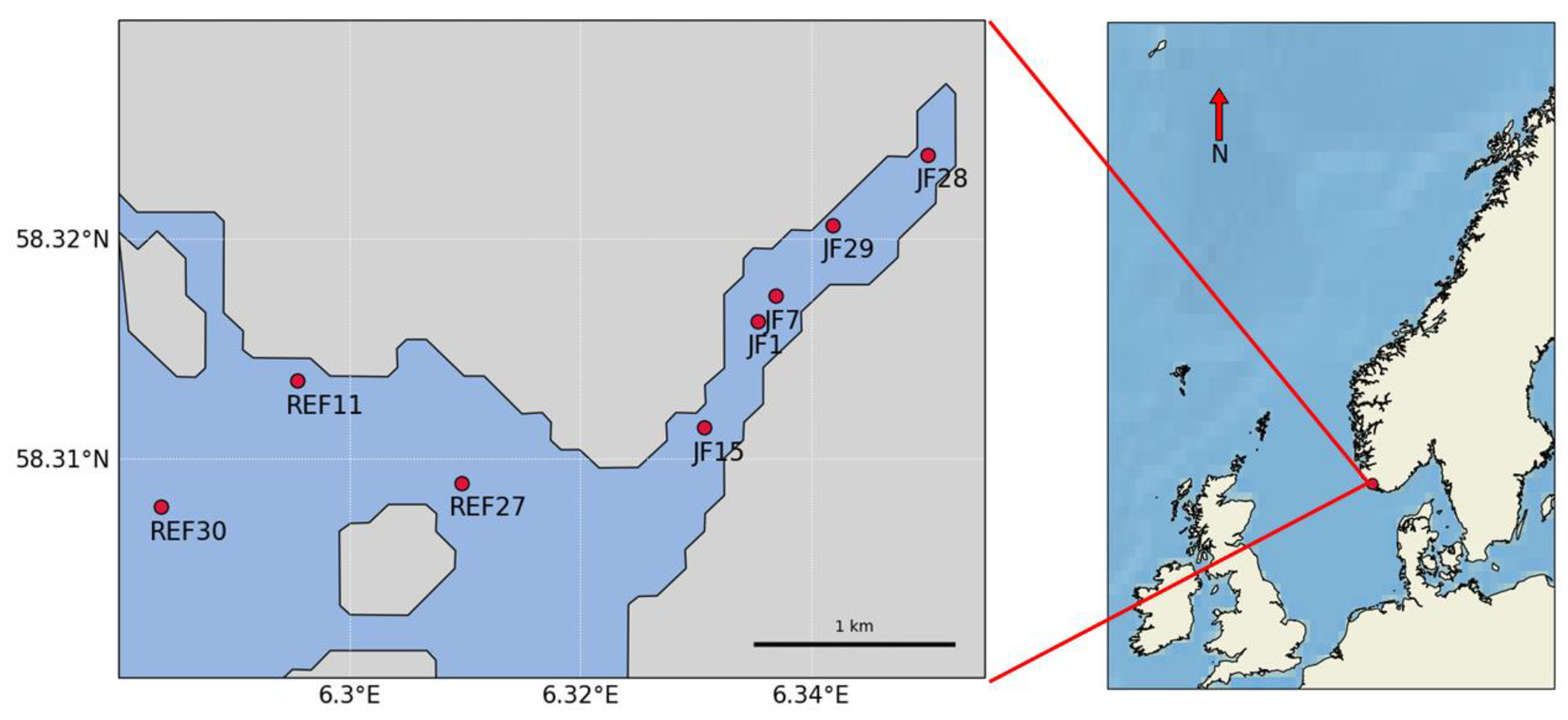
One of these sea deposits is the Jøssingfjord located in southwestern Norway, in the county of Rogaland, close to Egersund town (Figure 1). The length of the fjord is 3 km, and the width is about 250–300 m. It is surrounded by mountains oriented to the northeast.
Geologically the area consists of several large bodies of intrusive rocks in a magma chamber, collectively known as the Rogaland Anorthosite Province [17]. The province was formed during the Mesoproterozoic time, and the anorthosites were formed at 932–920 Ma [18,19].
The Rogaland Anorthosite Province contains numerous Fe-Ti oxide deposits, including the famous Tellnes ilmenite deposit [20]. The Tellnes deposit is fairly homogeneous, and the average composition is 53 vol. % euhedral plagioclase (An45–42), 29 vol. % interstitial hemo-ilmenite, and 10 vol. % orthopyroxene, with some Ti-biotite, olivine, and Fe-Ni-Co-Cu sulfides [18,21]. The ilmenite mineral (norite) in the Tellnes ore is a mixture of Fe- and Ti-oxides with small amounts of Fe-Ni-Co-Cu sulfides. Some of these sulfides are not produced and pass through to the tailings together with remnants of production chemicals such as tall oil, Xanthate, flocculants, and sulfuric acid [21,22]. Production was launched in 1916. Nowadays, it has the potential to continue for another 100 years at current production rates of about 3 million tons per year [15]. The tailings were disposed of in several deposits on land and in the sea in the Jøssingfjord and Dyngadjupet, off the southwest coast of Norway (Figure 1).
A major deposit was established in Jøssingfjorden during the period 1960–1984, when 2.5 × 10⁶ tons were deposited annually [23]. As a result, the depth was reduced from the maximum of 85 m to present depths close to the sill depth of 30 m [24]. After 1984, the discharge of tailings to the Jøssingfjord was significantly reduced. In 2016, about 1840 kg Ni was discharged to the inner part of Jøssingfjorden [25]. Suspended particles are also discharged to the inner part of Jøssingfjorden. In 2016, this amounted to 496 tons, most of which originated in drainage water pumped from the bottom of the mine [25]. Because of their different origin, the physical properties and mineral composition of these particles may be different from those of the tailings.
An assessment of mobilization and bioavailability of trace metals, essentially Ni, and potential impacts of tailings on the composition and functioning of the benthic ecosystem addressed as macrofauna communities and fluxes of O2 and nutrient species in the Jøssingfjord was recently made by Schaaning et al. [24]. The observations revealed higher Ni and Fe concentrations in the regions affected by tailings than in the baseline regions. Analysis of these observations results is needed to understand processes that lead to the present environmental state of the fjord and its potential future changes.
Models can be optimally used for numerical analyses of a system’s environmental state and for predictions of the possible changes. The goal of this work was to elaborate a model for simulations of cycling of Ni in the water column, the benthic boundary layer, and upper sediments (distributions, fluxes, rate of processes) and apply it to the case of abandoned mine tailing sea deposits in the Jøssingfjord.
The present work is a new version of the 1D benthic–pelagic coupled biogeochemical Bottom RedOx Model, BROM [26], supplemented with a Ni module specifically developed for the study (Figure 2). The model was optimized using field data collected in the Jøssingfjord. The fjord baseline water column, sediment biogeochemistry, and nickel cycling were simulated for the period before tailings disposal, during the intensive deposition of tailings, and during the restoration period after the stop of the intensive tailing deposition. Potential future dumping scenarios were numerically analyzed.
2. Materials and Methods
Here, we aim to model a specific environment of the fjord affected by the deposition of mine tailings, i.e., a mixture of gangue contaminated with leachates/precipitates settled onto the sediment, consisting of Si, Fe2O3, and NiS (see details in Section 2.4.2).
2.1. Model Description
This benthic–pelagic transport biogeochemical model BROM [26] combines a relatively simple ecosystem model with a detailed biogeochemical model for the water column, benthic boundary layer (BBL), and sediments, with a focus on oxygen and redox state. BROM consists of a 1-dimensional vertical transport module (BROM-transport) and a biogeochemical module (BROM-biogeochemistry) coupled through the Framework for Aquatic Biogeochemistry Model (FABM) [27].
BROM simulates a simple ecosystem composed of autotrophic (Phy) and heterotrophic (Het) organisms as well as four types of bacteria (aerobic heterotrophic and autotrophic bacteria and anaerobic heterotrophic and autotrophic bacteria).
BROM considers interconnected transformations of species (N, P, Si, C, O, S, Mn, Fe) and resolves organic matter (OM) in nitrogen currency. OM dynamics include parameterizations of OM production (via photosynthesis and chemosynthesis) and OM decay via oxic mineralization, denitrification, metal reduction, sulfate reduction, and methanogenesis, with a decreasing rate of OM decay in this sequence. To provide a detailed representation of changing redox conditions, OM in BROM is mineralized by several different electron acceptors, and dissolved oxygen is consumed during both mineralization of OM and oxidation of various reduced compounds. Organic matter is described in the model as dissolved labile, dissolved semilabile, particulate labile, and particulate semilabile OM. Following the approach of ERSEM [28], the decay of the labile forms results in the release of phosphate and ammonia and the transformation of labile forms into semilabile ones. During the decay of labile and semilabile OM, electron acceptors are consumed and carbon dioxide is released. Process inhibition in accordance with redox potential is parameterized by various redox-dependent switches. BROM also includes a module describing the carbonate equilibria; this allows BROM to be used to investigate acidification and impacts of changing pH and saturation states on water and sediment biogeochemistry. A detailed description of the model can be found in [26]. The source code and description are available at https://github.com/BottomRedoxModel (accessed on 27 March 2021). BROM-biogeochemistry code is divided into 20 different modules that can be used independently (brom_bio for ecosystem processes, brom_nitrogen for nitrogen species transformations, brom_fe for iron species transformations, etc.).
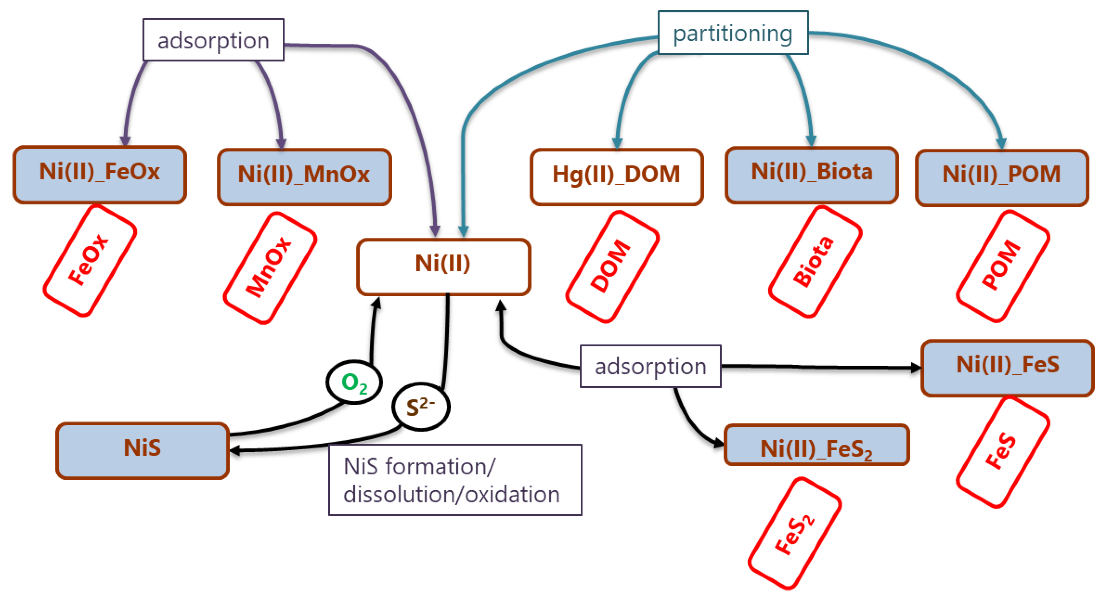
In this work, a new module, brom_ni, was elaborated. This module considers the transformation of different species of Ni in line with changes of other BROM variables (Figure 2). We parametrized reactions of Ni(II) and NiS (formation, dissolution, oxidation) and Ni(II) adsorption on oxides of Fe and Mn as well as on FeS and FeS2. We also parameterized Ni(II) partitioning with particulate and dissolved organic matter (labile POM and labile DOM) and its bioaccumulation by biota (Figure 2). Adsorption and bioaccumulation were parametrized according to Katsev et al. [29]. Bioaccumulation by biota includes autotrophs, heterotrophs, and all types of bacteria. The code of this module with the comments and the values of coefficients used is available at https://github.com/BottomRedoxModel/brom_niva_module/tree/master/brom (accessed on 27 March 2021).
2.2. Boundary Conditions
The model domain spans from the sea surface (upper boundary) down to 10 cm depth in the sediment (lower boundary). At the upper boundary, the fluxes of O2, CO2, NO3−, PO43−, Si, Fe(III) and Mn(IV) oxides, and Ni(II) were defined. Fluxes for all other modeled chemical constituents were set to zero. For CO2, the surface fluxes were calculated as proportional to the difference of their concentrations in the surface water and constant atmospheric concentrations of CO2 (380 ppmv). The exchange of O2 was parameterized as a function of O2 saturation in the surface water.
Inputs of PO43−, NO3−, Fe, and Mn from atmospheric deposition and coastal discharges were taken into account by setting constant or seasonally changeable concentrations on the water surface. There seasonal variability of inputs of PO43− and NO3− was parameterized. Maximum concentrations in the winter–spring period were assumed to be 1.6 μM for PO43− and 7 μM for NO3−. Minimum concentrations are assumed to be zero (depleted) in the summer period. Surface concentrations were set constant at 0.1 μM Fe(III), 0.1 μM Mn(IV), and 0.0001 μM Ni(II).
With an exception for alkalinity (Alk) and sulfate (SO42−), the concentrations at the lower boundary were calculated from the processes that occurred in the water column, BBL and upper sediment. Therefore, the model biogeochemistry is predominantly forced by the upper boundary conditions.
Besides this, the water column concentrations are “relaxed” (i.e., they change their values towards the “climate” data from a database) to account for lateral exchange with the open sea (following an approach described in [26]).
2.3. Hydrophysics
BROM-transport requires forcing for temperature, salinity, and turbulent vertical diffusivity at all depths in the water column and for each day of the simulation.
For the Jøssingfjord, we used the output from model ROMS [30]. The vertical diffusion coefficient kz was calculated based on vertical density distributions, following an approach by Gargett (1984) such that
where and represents the buoyancy frequency; a0 and q are empirical coefficients.
For the specific case of the Jøssingsfjord, values of a0 and q were set to 0.5 × 10⁻⁶ and 0.5, respectively. For theBBL, kz was assumed to be constant with a value of 0.5 × 10⁻⁶ m2 s−1.
In the sediments, kz was parameterized as a sum of the pore water molecular diffusion coefficient 1 × 10⁻¹¹ m2 s−1 and the bio-irrigation and sediment biomixing coefficient with a maximum value 0.1 × 10⁻¹¹ m2 s−1 in the upper 5 mm of the sediments and exponentially decreasing with the increase in depth, as described in Yakushev et al. [26]. Bioturbation occurs in cases where oxygen concentrations in the bottom water are higher than 5 μM.
2.4. Forcing
2.4.1. Water Column
We used nutrient and dissolved oxygen data from the World Ocean Database 2013 (WOD13) https://www.ncei.noaa.gov/products/world-ocean-database (accessed on 27 March 2021). WOD13 is the largest scientifically quality-controlled database of selected historical in situ surface and subsurface oceanographic measurements and is produced by the Ocean Climate Laboratory (OCL) at the National Oceanographic Data Center (NODC), Silver Spring, Maryland, USA. The analyzed dataset includes all data from the stations within the approximately 50 km distance from the mouth of the Jøssingfjord. Within this polygon, only the stations with depths less than 360 m and data starting from the year 1950 were included. All the imported data had quality flags of 0 (accepted value). The World Ocean Database 2013 (WOD13) database was used to set climatic seasonal relaxation data and upper boundary conditions for the water column [26].
2.4.2. Sediment
The data of observations [31] was used to set up low boundary conditions for alkalinity (4300 µM), sulfate (15,000 µM), and dissolved inorganic carbon (8000 µM).
2.4.3. Tailings
Analysis of the chemical composition of tailings shows that dominant fractions of solids are SiO2 (43.7%, weight percentages), Al2O3 (16.5%), and Fe2O3 (14.4%). The share of Ni is about 0.03% [32].
On the basis of these estimates we parameterized the modeled tailings as having a constant ratio between particulate Si, Fe2O3, and NiS as molar percentages of 76.86%, 23.06%, and 0.08%, respectively, assuming that modeled share of particulate Si includes parameters not considered in the model (i.e., salts of Al and Mg).
For the period of intensive tailing deposition, 1960–1984, we parameterized injection to the surface as a 50 × 50 m layer of 5 mmol Ni/s, which corresponds to the dumping of 2.3 million tons of suspended solids (SS) annually to all the fjord. After 1984, the injection was abruptly reduced to 0.0015 mmol Ni/sec; this corresponds to an annual supply to the fjord of 1550 kg of Ni and 699 tons of SS, which is close to the present-day discharge of 1840 kg of Ni and 496 tons of SS [25].
The simulations started from homogeneous initial conditions of all the parameters in the water column and the sediments. The model was spun up for 10 model years with repeated-year forcing and boundary conditions. After this time, a quasi-stationary solution with seasonally forced oscillations of the biogeochemical variables was reached.
2.5. Scenarios
Three different scenarios were modeled in addition to the main scenario:
- Total cessation of mine tailing deposition into the fjord in 2030.
- Doubling of the intensity of mine tailing deposition into the fjord in 2030.
- Increased bioturbation activity from 2020. Bioturbation activity was changed by an increase in parameters of sediment diffusivity (Table 1).
3. Results
3.1. Simulated Interannual Variability
The constructed model was applied for simulations of the benthic–pelagic systems under seasonally changing hydrophysical and biogeochemical forcing.
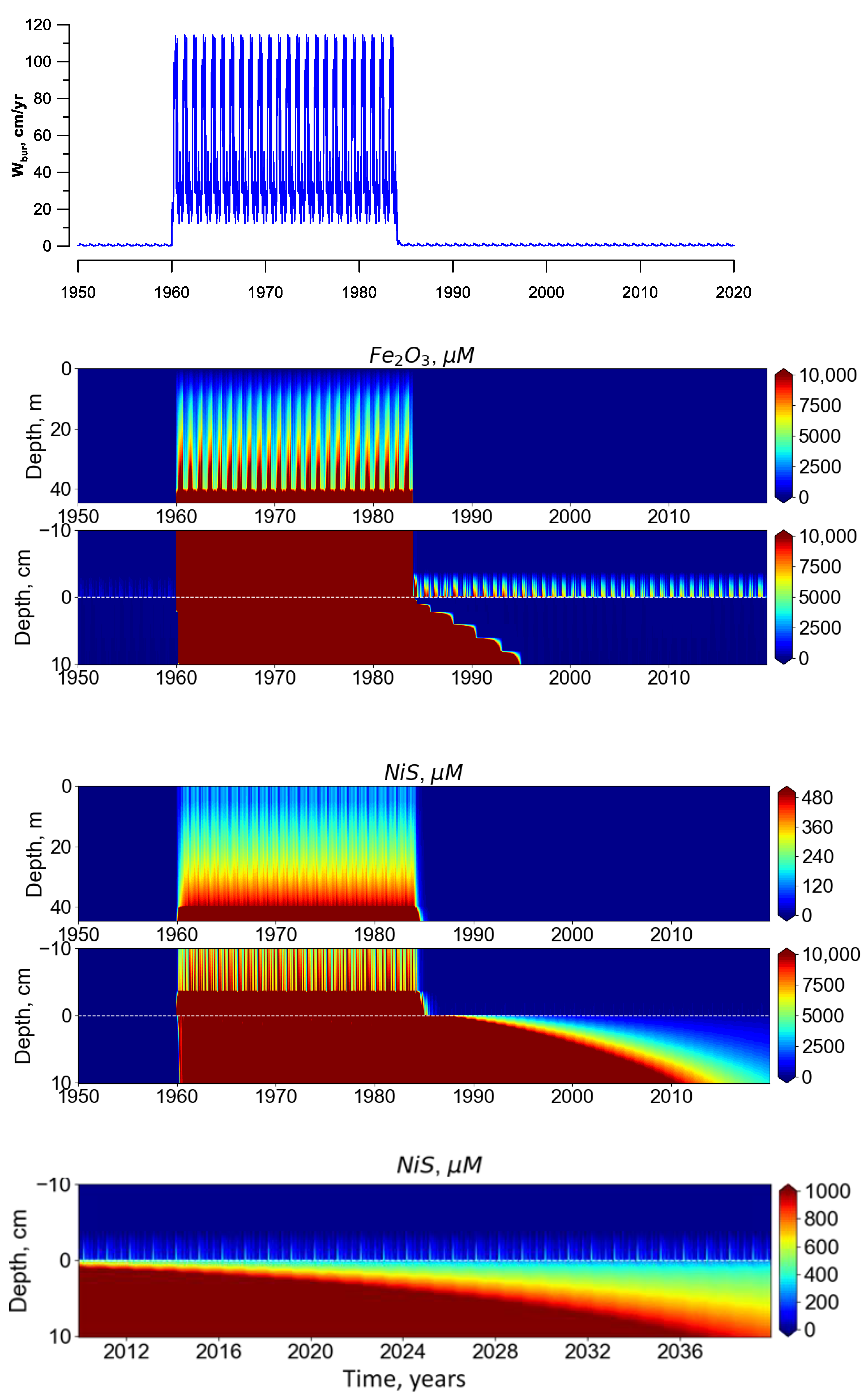
We first simulated the “baseline solution” for the system for conditions of the natural fjord seasonal variability with relatively low content of iron and nickel species entering the system and low burying rate (natural state (NS); model years 1940–1960, including the “spin-up” period 1940–1949 not shown in the figures). Then we simulated a 24-year period of high rates of deposition of tailings containing particulate Si, Fe2O3, and NiS (intensive deposition (ID); from 1960 to 1984). After 1984, restoration with the current low discharge (CLD) was modeled until 2040 (Figure 3). Burying velocity calculated in BROM depends on the amount of particulate matter that reaches the bottom. Therefore, during the period of natural conditions (years 1955–1960), the model reproduced the seasonal changes in burying velocity within the limits of 0.5–4.4 cm/year with a maximum following the period of synthesis of organic matter in the productive periods of the year. During the intensive tailing deposition, the burying rate oscillates within the limits of 30–130 cm/year, with an average value of about 50 cm/year. These oscillations can be explained by the seasonality of the mixing in the water column. During the winter period, an intense vertical mixing keeps the particles in suspended condition, while in the summer period under developed stratification, particles precipitate to the bottom. Therefore, the model predicted a 12-m decrease in the average depth of the fjord during the discharge period.
According to historic maps, the maximum depth decreased by 50 m from 80 to 30 m, so the decrease in the average depth predicted by the model appears realistic. After the intensive discharge was ended in 1984, the burying rate decreased to 0.6–4.5 cm/year, which is close to the predeposition rate. That means that the current small discharge did not contribute to a significant increase in the burying velocity.
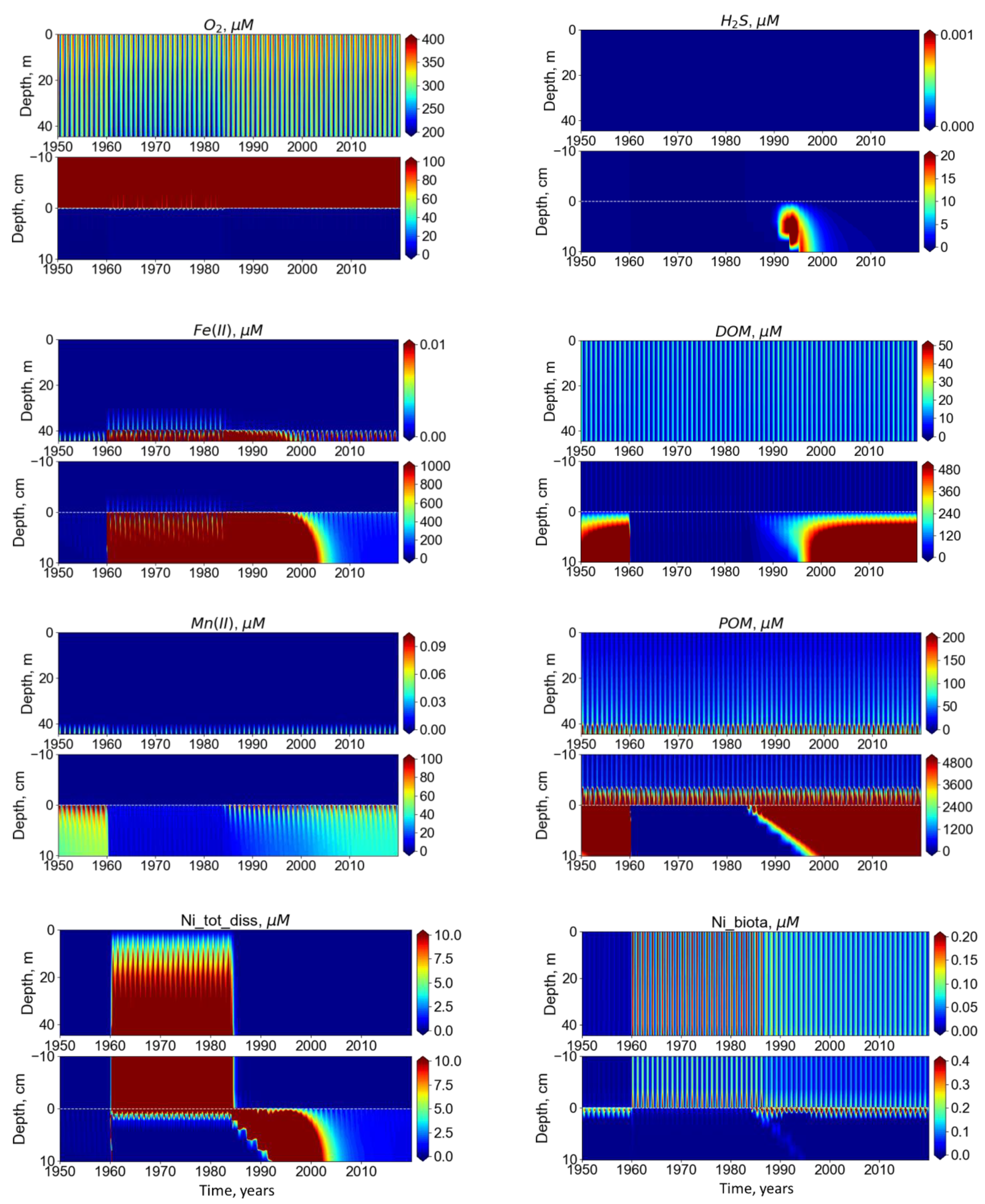
Intense deposition of mine tailings resulted in changes of biogeochemical composition both in the water column and the upper sediment layer. The oxygen concentration in the water column became about 10% lower, and the minimum O2 concentration in the bottom layer decreased from 150 to 100 µM (Figure 4). However, the high burying rate allowed some O2 (1–10 µM) to penetrate deeper into the sediment, i.e., down to 1 cm (Figure 4). Increased turbidity during the intense tailing deposition period led to changes in the model ecosystem, i.e., limitation of photosynthesis, decrease in organic matter, and disappearance of heterotrophs in the sediment. The concentrations of many dissolved (Mn(II), DOM) and solid (MnO2, POM) substances decreased in the sediment under intensive tailing, followed by an increase again after 1984 (Figure 4). The concentration of dissolved Fe(II) increased from 20–50 µM to 1–10 mM under intensive deposition from 1960. After the decrease in deposition rate, the concentration of Fe(II) reached an absolute maximum level of 30 mM, which was maintained for several years and was a result of the very intensive reductive dissolution of Fe(III) under oxidation of the restored high amount of OM and slow burial rate. Under these conditions, a low concentration of hydrogen sulfide (up to 25 µM) appeared in the porewater (Figure 4).
The concentration of total dissolved Ni in the water column increased from 0.009 to 20 µM under intensive tailing deposition, followed by a sharp decrease after 1984 to 0.06 µM (Figure 4). The concentration of total dissolved Ni in porewater increased significantly after intensive deposition was ended. Lower burial rate after 1984 allowed a high amount of NiS to remain available for oxidation in upper sediment layers; dissolution rate of NiS increased up to one order of magnitude and resulted in a concentration of total dissolved Ni in porewater of 50–200 µM until 1998. During the next 5 years, its concentration sharply decreased to 5 µM, and it did not exceed 2 µM after 2008. The concentration of NiS in the sediment decreased slowly after intensive deposition was ended. Even in 2020, its concentration was greater than 1000 µM below 4 cm depth and about 300–500 µM in the upper 4 cm (Figure 3). During NS conditions, the concentration of Ni in biota amounted to 0.01 µM in the water column and 0.4 µM in sediment. Maximum values of 0.24 µM for the water column and 1.3 µM for sediment were observed during the first 3 years after intensive deposition was ended. After 2008, the concentration of Ni in biota had a maximum of 0.12 µM in the water column and 1 µM in sediment.
3.2. Comparison with the Field Data
3.2.1. Porewater Concentrations
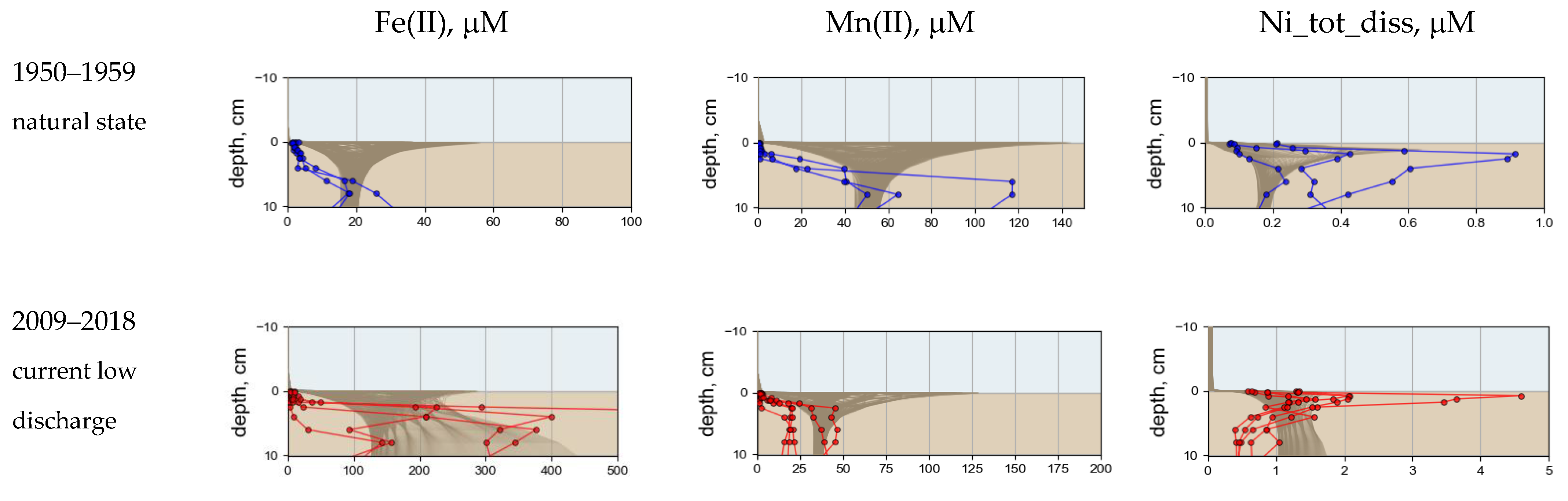
Comparisons of model results and observed field data are shown in Figure 5. The observations of dissolved Fe, Mn, and Ni distributions in the porewater were performed in the open sea (stations REF11, REF27, and REF30) and in the Jøssingfjord (stations JF5, JF7, JF11, JF28, and JF29) in 2015 [24] (Figure 1). Data for the open sea were taken to represent distributions before mine tailing deposition (natural state (NS)), and data in the fjord reflect a present state with low tailing deposition into the fjord (current low discharge (CLD)). According to the field data, concentrations of dissolved Fe and Ni are higher in the fjord than in the open sea, while the concentration of dissolved Mn is lower. This was consistent with high concentrations of solid Fe and Ni and low concentration of solid Mn in the tailings. Modeled porewater concentration levels of studied metals were consistent with the field data both for the period before mine tailing deposition and for the present day. High model concentrations of reduced Fe and Mn near the sediment surface result from the low penetration of O2 causing reduced Fe(II) and Mn(II) to be stable all the way up to the sediment surface. This is a typical distribution of Fe and Mn in many coastal and fjord sediments [34]. The distribution of dissolved Fe and Mn in the porewater has usual seasonality with maximum followed by high productivity period and intensive oxidation of OM by Fe and Mn oxides [35].
Modeled distribution of total dissolved Ni in porewater is characterized by a maximum at a sediment depth of 1–2 cm. According to the model, before 1960, for NS, the maximum concentration of total dissolved Ni did not exceed 0.009 µM in the water column and 0.6 µM in porewater. In 2009–2018, under CLD, the concentration of total dissolved Ni did not exceed 0.06 µM in the water column and 1.6 µM in porewater. Generally, modeled porewater distribution and concentration levels were reasonably consistent with the measured ones (Figure 5).
3.2.2. Benthic Fluxes
In a natural state without any input of Ni from the mining activity, the model calculations gave a benthic release flux of Ni varying over the year between 0.001 and 0.009 mmol/m2 day, 0.005 mmol/m2 day on average. At the current low discharge, the flux increased to 0.008–0.062 mmol/m2 day, 0.037 mmol/m2 day on average. Maximum fluxes occurred during the high production season. Field measurements of Ni benthic fluxes were carried out during low productivity and varied within the range 0.0004–0.0012 mmol/m2 day at reference stations and 0.003–0.010 mmol/m2 day in Jøssingfjord [24]. Another experiment with sediment covered by 2 cm of fresh Titania tailings showed release fluxes of dissolved Ni of 0.025–0.058 mmol/m2 day, 0.038 mmol/m2 day on average [25]. Thus, the modeled Ni release fluxes agreed reasonably well with the fluxes measured from tailings proper and at the deposit sites.
3.2.3. Ni in Sediment
Modeled concentration of Ni in the upper 10 cm of sediment for CLD amounted to 200–1000 µM (µmol Ni/L wet sediment) or 120–590 mg Ni/kg dry sediment. This agreed well with the observations of 115–200 mg/kg dw Ni in the upper 1 cm of sediment in Jøssingfjord [24].
If we accept that the modeled concentrations of dissolved Fe, Mn, and Ni, as well as NiS and Ni benthic fluxes, fit well to the field data, we can use the model to make predictions of further changes of Ni fate in the Jøssingfjord, for example, under different Ni discharge rates or intensity of bioturbation.
3.3. Numerical Experiments
3.3.1. Total Cessation of All Discharge of Mine Tailings
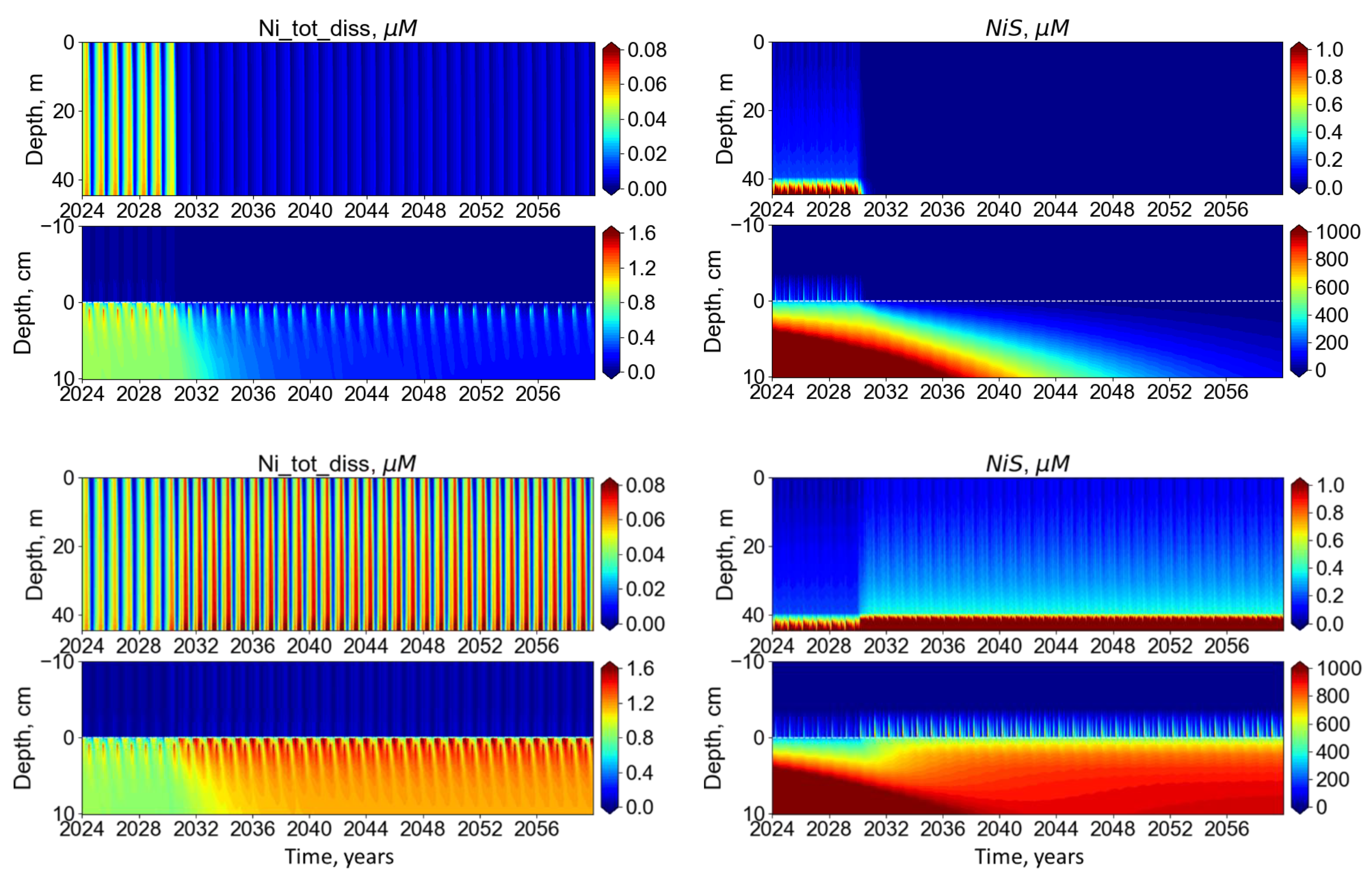
After the current low discharge was set to zero in 2030, the concentration of total dissolved nickel in the water column decreased significantly during the first two years (down to 0.01 µM), while its concentration in porewater returned to its natural state in about 10 years (Figure 6). The concentration of NiS in the top 5 cm of sediment decreased to below 100 µM in about 20 years after total cessation of tailings input.
3.3.2. Doubling of Deposition Intensity
After doubling the current low rate of Ni discharge, the annual average benthic flux of total dissolved Ni from the sediment increased from 0.037 to 0.051 mmol/m2 day. The maximum concentration of dissolved Ni reached 0.08 µM in the water column and 1.6 µM in porewater (Figure 6). The concentration of NiS remained at a relatively high level—about 500 µM in the upper 3 cm of sediment and about 900 µM down to 10 cm.
3.3.3. Increase in Bioturbation Activity
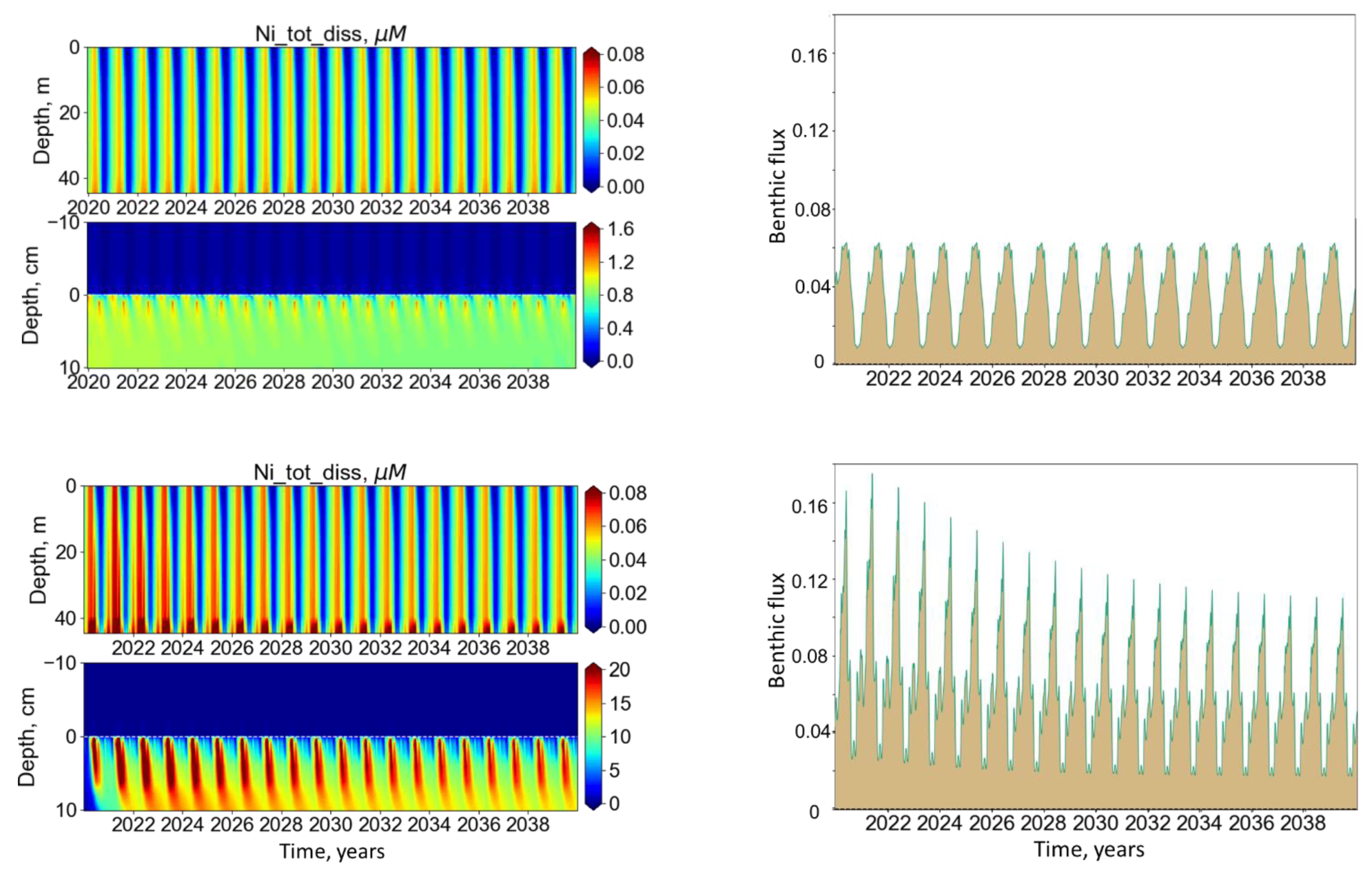
A numerical experiment with an increase in bioturbation that was initiated in 2020 clearly showed the importance of this factor for enhanced Ni leaching from sediment (Figure 7). After more active bioturbation was induced, dissolved Ni concentration increased from 0.06 to 0.15 µM in the water column, from 0.08 to 0.8 µM in BBL, and from 1.2 to 30 µM in porewater. The average annual benthic flux of dissolved Ni increased from 0.037 to 0.09 mmol/m2 day with a maximum of 0.18 mmol/m2 day. After 18–20 years, dissolved Ni concentration did not exceed 0.075 µM in the water column, 0.5 µM in BBL, and 20 µM in porewater. In this long-term perspective, the average Ni benthic flux decreased to 0.06 mmol/m2 day.
4. Discussion
In this paper, we have described an application of a mathematical model for analyzing the fate of nickel leaching from a sea deposit of mine tailings. In our model, we considered how the processes in the water column, the benthic boundary layer (BBL), and the sediments were affected by a simulated seasonality of production–decay processes of organic matter.
4.1. Ni Species Fate
In summary, we can describe the following features of the Ni transformation:
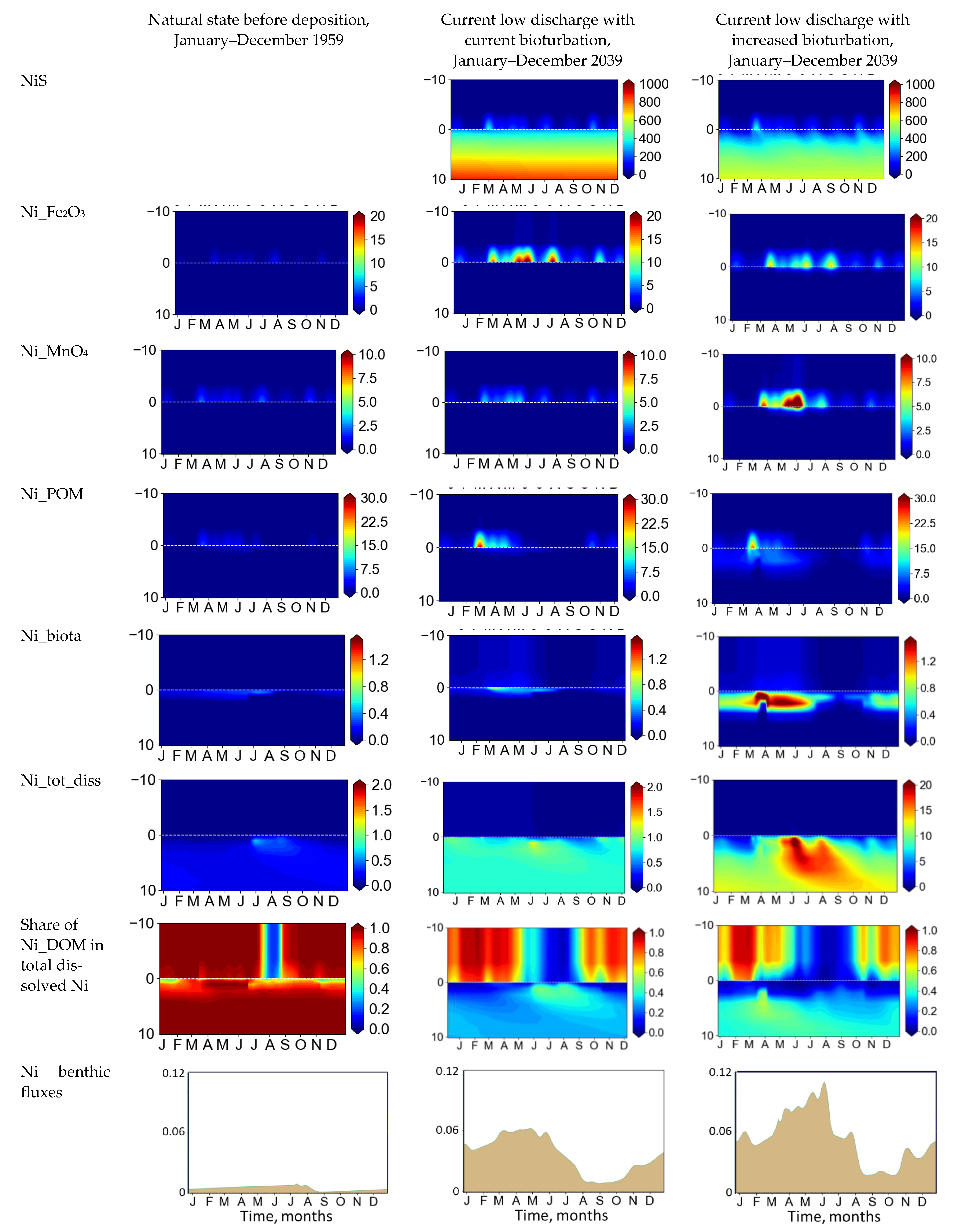
In natural conditions, Ni is characterized by low concentrations both in the water column (0.009 µM) and in porewater (maximum 0.6 µM). Practically all Ni is associated with DOM (Figure 8). The highest concentration of total dissolved Ni was observed in summer when active oxidation/reduction processes took place, resulting in desorption of Ni2+ adsorbed on Fe2O3, MnO2, and POM under their oxidative/reductive dissolution. Release of Ni to the bottom water followed the maximum concentration of Ni adsorbed on these suspended particles (Figure 8). In the natural condition, the model showed a significant seasonal variation of the benthic release flux of Ni following the annual OM formation/decay processes.
Under the current low discharge of mine tailings, Ni was assumed to enter the fjord in the form of particulate NiS. The oxidation and dissolution of discharged Ni led to the release of Ni2+ to the water, followed by its adsorption mainly on Fe2O3 and POM. Thus, Ni_POM and Ni_Fe2O3 concentrations increased 5 and 10 times, respectively, compared to the natural conditions without any discharge from the mining activity (Figure 8). The maximum concentration of total dissolved Ni occurred in the summer period after the dissolution of POM and Fe2O3 and desorption of Ni2+. Total dissolved Ni concentration in the water column was 6 times higher (0.06 µM) than in natural conditions, and porewater concentration was 2 times higher (1.2 µM) (Figure 8). Benthic release of Ni increased 6 times to 0.06 mmol/m2 day as maximum and reached 0.037 mmol/m2 day on average. The share of dissolved Ni associated with DOM decreased in comparison to the situation before the deposition, especially in porewater. The concentration of Ni in biota increased 2.5–10 times under current low deposition in comparison with the natural state.
An increase in bioturbation activity resulted in the intensification of oxidation and reduction processes in the upper sediment. The amount of NiS in the upper sediment decreased significantly in comparison to the low bioturbation conditions (Figure 8) because of active oxidation. The concentration of Fe2O3 remained practically at the same level because of its constant input with tailings, while the concentrations of Fe2+, MnO2, and Mn2+ increased one order of magnitude as a result of intensive diagenesis [35,36]. The concentration of total dissolved Ni in the porewater increased to 22 µM due to enhanced downwards mixing of O2 for the oxidation of NiS. In the water column, the concentration of dissolved Ni increased to a maximum of 0.15 µM shortly after the induction of intensive bioturbation, and this was followed by a decrease to 0.06 µM. The benthic flux of total dissolved Ni first increased 3 times to a maximum of 0.18 mmol/m2 day, followed by a decline to 0.12 mmol/m2 day (Figure 7). Notably, the increase in Ni in porewater did not result in an increase in the benthic flux to the same extent, because most of the released Ni was adsorbed on Fe and Mn oxides and POM. Meanwhile, the concentration of Ni in biota increased up to 100 times under intense bioturbation in comparison with current low deposition conditions.
Schaanning et al. [24] showed that sediment concentrations in the top layer (0–1 cm) of the sediments remained elevated for more than 20 years after the deposition was ended in the open area (Dyngadjupet) and explained this by upwards mixing of tailings enhanced by the high density of conveyor belts and other bioturbators in the area. Near-surface oxidation of recycled metal sulfides caused increased concentrations of metals in pore water and elevated fluxes from the sediments to the overlying water. Consistent with the relatively high loss of Ni, they also showed that the Ni/Cu ratio decreased from about 2:1 in the tailings and deep deposit layers to about 1:1 in the top layer (Figure 2A in Schaanning et al., 2019). The BROM model was able to reproduce this complex mechanism and demonstrated that bioturbation has a large potential to postpone restoration of predeposition conditions with NS metal spreading to surrounding environments and biota.
4.2. Environmental Status of Water and Sediment in Jøssingfjord for Different Scenarios
Compared to the Norwegian Quality Standards [37], the calculated concentrations of dissolved Ni in the natural state correspond to the quality classes “very good” in the water column, BBL, and, sediment and “moderate” in pore water (Table 2). At present-day low discharge, concentrations correspond to “good” in the water column and BBL and “poor” in porewater and sediment (Table 2). The upper 10 cm of the sediments remained “poor” until 2040, while the upper 1 cm of sediment reached the “moderate” condition at about 2030 (Figure 3).
The model predicted that complete cessation of the discharges would result in an improvement of sediment state to “good” in about 5–7 years for the top 1 cm layer and in about 22 years for the top 10 cm of sediment. (Figure 6). Ten years after ending the deposition of tailings, porewater was predicted to improve from “poor” to “moderate” state. Doubling of deposition intensity did not change status in the water column or porewater but caused the sediments to approach the boundary of “very poor” (Figure 6).
Increased bioturbation led to the change of the BBL and porewater conditions to “poor” and “very poor”, while sediment state improved to “moderate” (Table 2, Figure 8). This clearly demonstrates that an increase in bioturbation activity can worsen the environmental status of the Jøssingfjord provided that the concentration of Ni in sediment stays at a high level.
The application of the model described in this paper allowed numerical analysis of the fate of Ni under abundant mine tailing deposition to be performed. It was possible to reveal specific features of its transformation (i.e., role of bioturbation) and perform numerical experiments on future changes. The application of a complex biogeochemical benthic–pelagic coupled model for these purposes is a new perspective methodology, but naturally, there are limitations associated with the model development, application, and validation. We hope that we have taken into account all the important processes, but further studies are needed, and a similar approach can be used for analyzing the fate of other chemical elements (e.g., Cu and Co) found in these tailings.
5. Conclusions
A 1D benthic–pelagic coupled biogeochemical model, BROM, supplemented with an elaborated Ni module was applied for analyzing the Ni fate in the Jøssingfjord, which hosts an abundant mine tailing deposit and is affected by the current-day Ni waste discharge. The model was satisfactorily validated against the measurements. The model demonstrated that two decades are required to return the fjord’s sediment state to conditions close to natural conditions before the discharge of tailings. Transformations of dissolved Ni are connected with the formation and decay of OM, resulting in significant seasonal changes in Ni benthic flux. Bioturbation intensity plays a large role in the leaching of Ni from the sediment. The model can be an instrument for analysis of different scenarios for mine tailing activities from point of view of reduction of environmental impact as a component of the best available technology.
Author Contributions
Conceptualization, S.P., M.T.S., and E.Y.; methodology, E.Y.; software, S.P. and E.Y.; validation, S.P. and E.Y.; resources, M.T.S.; writing—original draft preparation, S.P. and E.Y., writing—review and editing, S.P., E.Y., and M.T.S. All authors have read and agreed to the published version of the manuscript.
Funding
M.T.S. and E.Y. were supported under the NYKOS project “New Knowledge On Sea Deposits” funded by the Norwegian Research Council (project No. 236658), S.P. and E.Y. were supported by the Norwegian Research Council project No. 272749 (“Aquatic Modeling Tools”, SkatteFUNN), and S.P. and E.Y. were supported by the Ministry of Science and Higher Education of Russia (theme 0128-2021-0001).
Data Availability Statement
Model outputs (netcdf) will be available on zenodo.org, accessed on 1 February 2021.
Acknowledgments
Authors are grateful to Elizaveta Protsenko (NIVA) and Anfisa Berezina (SIO RAS) for technical support with data visualization.
Conflicts of Interest
The authors declare no conflict of interest.
References
- Koski, R.A. Metal Dispersion Resulting from Mining Activities in Coastal Environments: A Pathways Approach. Oceanography 2012, 25, 170–183. [Google Scholar] [CrossRef]
- Ramirez-Llodra, E.; Trannum, H.C.; Evenset, A.; Levin, L.A.; Andersson, M.; Finne, T.E.; Hilario, A.; Flem, B.; Christensen, G.; Schaanning, M.; et al. Submarine and deep-sea mine tailing placements: A review of current practices, environmental issues, natural analogs and knowledge gaps in Norway and internationally. Mar. Pollut. Bull. 2015, 97, 13–35. [Google Scholar] [CrossRef]
- Reichl, C.; Schatz, M.; Zsak, G. World-Mining-Data. Miner. Prod. Inter Natl. Organ. Comm. World Min. Congr. 2014, 32, 1–261. [Google Scholar]
- Hudson-Edwards, K.A.; Dold, B. Mine Waste Characterization, Management and Remediation. Minerals 2015, 5, 82–85. [Google Scholar] [CrossRef] [Green Version]
- Arnesen, R.T.; Bjerkeng, B.; Iversen, E.R. Comparison of model predicted and measured copper and zinc concentrations at three Norwegian underwater tailings disposal sites. In Proceedings of the Fourth International Conference on Acid Rock Drainage, Vancouver, BC, Canada, 31 May–6 June 1997; Volume 4, pp. 1831–1847. [Google Scholar]
- Dold, B. Evolution of Acid Mine Drainage Formation in Sulphidic Mine Tailings. Minerals 2014, 4, 621–641. [Google Scholar] [CrossRef] [Green Version]
- Dold, B. Submarine tailings disposal (STD)—A review. Minerals 2014, 4, 642–666. [Google Scholar] [CrossRef]
- Simpson, S.L.; Spadaro, D.A. Bioavailability and Chronic Toxicity of Metal Sulfide Minerals to Benthic Marine Invertebrates: Implications for Deep Sea Exploration, Mining and Tailings Disposal. Environ. Sci. Technol. 2016, 50, 4061–4070. [Google Scholar] [CrossRef]
- Schippers, A. Biogeochemistry of metal sulfide oxidation in mining environments, sediments, and soils. In Sulfur Biogeochemistry—Past and Present; Geological Society of America Special Paper; Amend, J.P., Edwards, K.J., Lyons, T.W., Eds.; Geological Society of America: Boulder, CO, USA, 2004; Volume 379, pp. 49–62. [Google Scholar]
- Schaanning, M.T.; Trannum, H.C.; Pinturier, L.; Rye, H. Metal Partitioning in Ilmenite- and Barite-Based Drill Cuttings on Seabed Sections in a Mesocosm Laboratory. SPE Drill. Complet. 2011, 26, 268–277. [Google Scholar] [CrossRef]
- Koski, R.A.; Munk, L.; Foster, A.L.; Shanks, W.C.; Stillings, L.L. Sulfide oxidation and distribution of metals near abandoned copper mines in coastal environments, Prince William Sound, Alaska, USA. Appl. Geochem. 2008, 23, 227–254. [Google Scholar] [CrossRef]
- Amato, E.D.; Simpson, S.L.; Remaili, T.M.; Spadaro, D.A.; Jarolimek, C.V.; Jolley, D.F. Assessing the Effects of Bioturbation on Metal Bioavailability in Contaminated Sediments by Diffusive Gradients in Thin Films (DGT). Environ. Sci. Technol. 2016, 50, 3055–3064. [Google Scholar] [CrossRef]
- Mil-Homens, M.; Vale, C.; Naughton, F.; Brito, P.; Drago, T.; Anes, B.; Raimundo, J.; Schmidt, S.; Caetano, M. Footprint of roman and modern mining activities in a sediment core from the southwestern Iberian Atlantic shelf. Sci. Total Environ. 2016, 571, 1211–1221. [Google Scholar] [CrossRef]
- Simpson, S.L.; Apte, S.C.; Batley, G.E. Effect of Short-Term Resuspension Events on Trace Metal Speciation in Polluted Anoxic Sediments. Environ. Sci. Technol. 1998, 32, 620–625. [Google Scholar] [CrossRef]
- Berg, B.I.; Sæland, F.; Nyland, A.J.; Østensen, P.Ø.; Nordrum, F.S.; Kullerud, K. Bergverk i Norge; Fagbokforl: Bergen, Norway, 2016. [Google Scholar]
- Kvassnes, A.J.S.; Iversen, E. Waste sites from mines in Norwegian fjords. Mineralproduksjon 2013, 3, A27–A38. [Google Scholar]
- Nordgulen, Ø.; Andersen, A. Jordas Urtid–De Eldste Bergarter Dannes: 4600–850 MA; Ramberg, B., Bryhni, I., Nøttevedt, A., Eds.; Norges Geologi: Trondheim, Norway, 2007; pp. 107–108. [Google Scholar]
- Bjerkgard, T.; Boyd, R.; Ihlen, P.; Korneliussen, A.; Nilsson, L.P.; Often, M.; Sandstad, j.; Eilu, P.; Hallberg, A. Metallogenic areas in Norway. Geol. Surv. Finl. 2012, 53, 35–138. [Google Scholar]
- Schärer, U.; Wilmart, E.; Duchesne, J.C. The short duration and anorogenic character of anorthosite magmatism: U-Pb dating of the Rogaland complex, Norway. Earth Planet. Sci. Lett. 1996, 139, 35–350. [Google Scholar] [CrossRef]
- Charlier, B.; Skår, Ø.; Korneliussen, A.; Duchesne, J.-C.; Auwera, J.V. Ilmenite composition in the Tellnes Fe–Ti deposit, SW Norway: Fractional crystallization, postcumulus evolution and ilmenite–zircon relation. Contrib. Miner. Pet. 2007, 154, 119–134. [Google Scholar] [CrossRef]
- Duchesne, J.C.; Schiellerup, H. The iron-titanium deposits. In The Rogaland Intrusive Massifs: An Excursion Guide; NGU Report 2001.29; Duchesne, J.C., Ed.; Norges Geologiske Undersøkelse: Trondheim, Norway, 2001; pp. 56–75. [Google Scholar]
- Anon. Titania A/S–Proposal for Monitoring Program. Geode Consult AS, P.O. Box 97, 1378 Nesbu. 2015. [Google Scholar]
- Sørby, H.; Storbråten, G.; Braastad, G.; Løkeland, M. Bergverk og Avgangsdeponering. In Status, Miljøutfordringer og Kunnskapsbehov; Klif report TA2715/2010; Klima-og Forurensningsdirektoratet: Oslo, Norway, 2010. [Google Scholar]
- Schaanning, M.T.; Trannum, H.C.; Øxnevad, S.; Ndungu, K. Benthic community status and mobilization of Ni, Cu and Co at abandoned sea deposits for mine tailings in SW Norway. Mar. Pollut. Bull. 2019, 141, 318–331. [Google Scholar] [CrossRef] [PubMed]
- Fauske, L.L. Transport of Heavy Metals from Mine Waste of Titania. Master’s Thesis, University of Oslo, Oslo, Norway, 2017. [Google Scholar]
- Yakushev, E.V.; Protsenko, E.A.; Bruggeman, J.; Wallhead, P.; Pakhomova, S.V.; Yakubov, S.K.; Bellerby, R.G.J.; Couture, R.-M. Bottom RedOx Model (BROM v.1.1): A coupled benthic–pelagic model for simulation of water and sediment biogeochemistry. Geosci. Model Dev. 2017, 10, 453–482. [Google Scholar] [CrossRef] [Green Version]
- Bruggeman, J.; Bolding, K. A general framework for aquatic biogeochemical models. Environ. Model. Softw. 2014, 61, 249–265. [Google Scholar] [CrossRef] [Green Version]
- Butenschön, M.; Clark, J.; Aldridge, J.N.; Allen, J.I.; Artioli, Y.; Blackford, J.; Bruggeman, J.; Cazenave, P.; Ciavatta, S.; Kay, S.; et al. ERSEM 15.06: A generic model for marine biogeochemistry and the ecosystem dynamics of the lower trophic levels. Geosci. Model Dev. 2016, 9, 1293–1339. [Google Scholar] [CrossRef] [Green Version]
- Katsev, S.; Sundby, B.; Mucci, A. Modeling vertical excursions of the redox boundary in sediments: Application to deep basins of the Arctic Ocean. Limnol. Oceanogr. 2006, 51, 1581–1593. [Google Scholar] [CrossRef] [Green Version]
- Shchepetkin, A.F.; McWilliams, J.C. The regional oceanic modeling system (ROMS): A split-explicit, free-surface, topography-following-coordinate oceanic model. Ocean Model. 2005, 9, 347–404. [Google Scholar] [CrossRef]
- Gravdal, J.K.S. Stability of Heavy Metals in Submarine Mine Tailings: A Geochemical Study. Master’s Thesis, University of Bergen, Bergen, Norway, 2013. [Google Scholar]
- Mellgren, A. Dissolved Nickel in the Lundetjern land Deposit-Identification of Main Causes and Methods for Treatment. Master’s Thesis, Norwegian University of Science and Technology, Trondheim, Norway, 2002. [Google Scholar]
- Soetaert, K.; Middelburg, J.J. Modeling eutrophication and oligotrophication of shallow-water marine systems: The importance of sediments under stratified and well-mixed conditions. In Eutrophication in Coastal Ecosystems; Springer: Berlin/Heidelberg, Germany, 2009; pp. 239–254. [Google Scholar]
- Pakhomova, S.V.; Hall, P.O.; Kononets, M.Y.; Rozanov, A.G.; Tengberg, A.; Vershinin, A.V. Fluxes of iron and manganese across the sediment–water interface under various redox conditions. Mar. Chem. 2007, 107, 319–331. [Google Scholar] [CrossRef]
- Canfield, D.E.; Thamdrup, B.; Hansen, J.W. The anaerobic degradation of organic matter in Danish coastal sediments: Iron reduction, manganese reduction, and sulfate reduction. Geochim. Cosmochim. Acta 1993, 57, 3867–3883. [Google Scholar] [CrossRef]
- Silverberg, N.; Sundby, B. Sediment-Water Interaction and Early Diagenesis in the Laurentian Trough. In Oceanography of a Large-Scale Estuarine System; Springer: Berlin/Heidelberg, Germany, 1990; pp. 202–238. [Google Scholar]
- Veileder 02:2018 Klassifisering av Miljøtilstand i vann. Økologisk og Kjemisk Klassifiseringssystem for Kystvann, Grunnvann, Innsjøer og Elver. Direktoratsguppen Vanndirektivet. 2018. Available online: https://www.vannportalen.no/veiledning/klassifiserings/ (accessed on 1 February 2021).
Figure 1.
Position of stations in the Jøssingfjord (stations JF15, JF1, JF7, JF29, and JF28) and in the open sea (REF11, REF27, and REF30).
Figure 1.
Position of stations in the Jøssingfjord (stations JF15, JF1, JF7, JF29, and JF28) and in the open sea (REF11, REF27, and REF30).

Figure 2.
Nickel transformations in aquatic ecosystems parametrized in the brom_ni module. Brown rectangles correspond to the state variables in the brom_ni module, red rectangles correspond to the state variables of BROM, whose concentrations are used in calculations of Ni transformations. Uni-directional arrows reflect the processes considered in the model. Open brom_ni rectangles represent dissolved species and shaded ones represent particulate species. The processes occur both in the pelagic and benthic parts of the model.

Figure 3.
Interannual variability of the burying rate and Fe2O3 and NiS concentrations (µmol/L wet sediment).
Figure 3.
Interannual variability of the burying rate and Fe2O3 and NiS concentrations (µmol/L wet sediment).

Figure 4.
Modeled interannual variability of concentration (µM) of dissolved O2, Fe(II), Mn(II), DOM, H2S, POM, total dissolved Ni, and bioaccumulated Ni.
Figure 4.
Modeled interannual variability of concentration (µM) of dissolved O2, Fe(II), Mn(II), DOM, H2S, POM, total dissolved Ni, and bioaccumulated Ni.

Figure 5.
Vertical distributions of dissolved Fe(II) and Mn(II) and total dissolved Ni simulated for different periods (brown lines) and observed in 2015 in the fjord (red circles ) and the open regions (blue circles).
Figure 5.
Vertical distributions of dissolved Fe(II) and Mn(II) and total dissolved Ni simulated for different periods (brown lines) and observed in 2015 in the fjord (red circles ) and the open regions (blue circles).

Figure 6.
Modeled interannual variability of total dissolved nickel (left) and NiS (right) concentrations after total cessation (top) or doubling (bottom) of the current low deposition rate discharge in 2030.
Figure 6.
Modeled interannual variability of total dissolved nickel (left) and NiS (right) concentrations after total cessation (top) or doubling (bottom) of the current low deposition rate discharge in 2030.

Figure 7.
Modeled interannual variability of total dissolved nickel concentration (μM, left) and its benthic release flux (mmol/m3 day, right) for present-day bioturbation intensity (top) and in case of increased intensity of bioturbation from 2020 (bottom).
Figure 7.
Modeled interannual variability of total dissolved nickel concentration (μM, left) and its benthic release flux (mmol/m3 day, right) for present-day bioturbation intensity (top) and in case of increased intensity of bioturbation from 2020 (bottom).

Figure 8.
Modeled seasonal variability of concentrations of NiS, Ni adsorbed on Fe2O3 and MnO2, Ni associated with POM, bioaccumulated Ni, and total dissolved Ni (μM) and share of Ni_DOM in total dissolved Ni (%) and Ni benthic release flux (mmol/m3day): natural state before deposition (left), current low discharge with low bioturbation (middle), and current low discharge with increased bioturbation (right).


Table 1.
Parametrization of bioturbation activity for different scenarios.
| . | Basic Scenario | Increased Bioturbation Scenario |
|---|---|---|
| kz_bioturb_max, m2/s | 1 × 10⁻¹¹ | 20 × 10−11 |
| z_const_bioturb, m | 0.0001 | 0.01 |
| z_decay_bioturb, m | 0.01 | 0.1 |
kz_bioturb_max is maximum diffusivity due to bioturbation in the sediments, range (0.3–30) × 10−11 m2/s [33]; z_const_bioturb is the thickness of the sediment layer with maximum diffusivity, range 0.01–0.05 m [33]; z_decay_bioturb is the decay scale of bioturbation diffusivity below z_const_bioturb; value 0.01m [33].
Table 2.
Environmental Quality Standards (EQS) for nickel in coastal water and sediments [37] and environmental conditions of the Jøssingfjord under different modeled scenarios.
Table 2.
Environmental Quality Standards (EQS) for nickel in coastal water and sediments [37] and environmental conditions of the Jøssingfjord under different modeled scenarios.
| Condition | Class I Background “Very Good” | Class II AA-EQS “Good” | Class III Mac-EQS “Moderate” | Class IV “Poor” | Class V “Very Poor” |
|---|---|---|---|---|---|
| Coastal water, μg/L (μM) | <0.5 (0.01) | 0.5–8.6 (0.01–0.15) | 8.6–34 (0.15–0.58) | 34–67 (0.58–1.14) | >67 (1.14) |
| Sediment, mg/kg | <30 | 30–42 | 42–271 | 271–533 | >533 |
| Water column | NS | CLD, CLDib | ID | ||
| BBL (water) | NS | CLD | CLDib | ID | |
| Porewater | NS | CLD | CLDib | ||
| Sediment | NS | CLDib | CLD | ID |
NS, natural state; ID, intensive mine tailing deposition (1960–1984); CLD, current low discharge with present bioturbation; CLDib, current low discharge with increased bioturbation.
Publisher’s Note: MDPI stays neutral with regard to jurisdictional claims in published maps and institutional affiliations. |
© 2021 by the authors. Licensee MDPI, Basel, Switzerland. This article is an open access article distributed under the terms and conditions of the Creative Commons Attribution (CC BY) license (https://creativecommons.org/licenses/by/4.0/).
Share and Cite
MDPI and ACS Style
Pakhomova, S.; Yakushev, E.; Schaanning, M.T. Modeling Nickel Leaching from Abandoned Mine Tailing Deposits in Jøssingfjorden. Water 2021, 13, 967. https://doi.org/10.3390/w13070967
AMA Style
Pakhomova S, Yakushev E, Schaanning MT. Modeling Nickel Leaching from Abandoned Mine Tailing Deposits in Jøssingfjorden. Water. 2021; 13(7):967. https://doi.org/10.3390/w13070967
Chicago/Turabian StylePakhomova, Svetlana, Evgeniy Yakushev, and Morten Thorne Schaanning. 2021. "Modeling Nickel Leaching from Abandoned Mine Tailing Deposits in Jøssingfjorden" Water 13, no. 7: 967. https://doi.org/10.3390/w13070967
Note that from the first issue of 2016, this journal uses article numbers instead of page numbers. See further details here.