Analytical Solution of Saltwater Intrusion in Costal Aquifers Considering Climate Changes and Different Boundary Conditions

Abstract

Groundwater contamination due to saltwater intrusion (SWI) has an extreme effect on freshwater quality. Analytical and numerical models could be used to investigate SWI. This study aims to develop an analytical solution to investigate SWI into coastal aquifers which was applied to a real case study at the Middle Nile Delta aquifer (MNDA). The study presented a new formula to predict the difference in depth of freshwater to seawater interface due to a change in boundary conditions. A Computer Program for Simulation of Three-Dimensional Variable-Density Ground-Water Flow and Transport (SEAWAT) is used for groundwater flow simulation and SWI and the results compared with the developed analytical solution. Four scenarios are considered in the study, including; the sea-level rise (SLR), reduction in recharge, over abstraction, and combination after 50 years (2070). The analytical solution gave good results compared to the numerical one where Equiline 1 intruded to 103 and 101.66 km respectively at the base case. The results also gave a good agreement between numerical and the analytical solution for SLR due to climate changes by 52.80 cm where the Equiline 1 reached to 105 and 103.45 km. However, the reduction in aquifer recharge by 18.50% resulted in an intrusion for the Equiline-1 to 111 and 108.25 km from the shoreline. Over pumping due to the increase in population by 89% has increased the SWI to reach 121,110.31 km, while it reached 131 and 111.32 km at a combination of the three scenarios, which represents the highest threatening scenario. Also, the difference between the two solutions reached 1.30%, 1.48%, 2.48%, 8.84%, and 15.02%, respectively for the base case and four scenarios. For the current case study, the analytical model gave good results compared to the numerical one, so that the analytical solution is recommended for similar studies, which could save the time and capabilities of computer required for the numerical solutions.

1. Introduction

Coastal aquifers are the main source of freshwater resources in many countries over the world [1]. A number of coastal areas around the world are subject to saltwater intrusion (SWI) which resulted in deterioration of groundwater [2]. SWI is an environmental problem in coastal areas where more than two third of the world’s population lives. This problem is mainly due to indiscriminate and unplanned abstraction of groundwater from these aquifers that are hydraulically connected with the sea [3]. In these aquifers, the denser saline water tends to remain separated from the overlying freshwater forming a variable density miscible fluid mixing zone called a transition or dispersion zone [4]. Saline water is dynamic flows in a cycle from the floor of the sea to the zone of dispersion and back to the sea [5].

During the previous century, field measurements showed that the global mean Sea-Level Rise (SLR) has increased from 10 to 20 mm per year according to the Intergovernmental Panel on Climate Change (IPCC) in 1996. By 2100, the SLR is expected to increase at a rate between 90 to 880 mm per year according to IPCC (2001) [6], while it was estimated between 180 and 580 mm based on IPCC in 2007. Klein and Lichter [7] showed that the average rate of SLR in the Mediterranean Sea ranges from 0.50 to 2.5 mm/year while IPCC (2014) [8] indicated that the SLR changed from 1.70 to 2.30 mm/year over the 20th century. Also, IPCC (2014) [8] showed that the precipitation has increased since 1901 at the mid-latitude land areas of the Northern Hemisphere while other latitudes have long-term positive or negative trends. Moreover, the future changes in rainfall will be variable, the high latitudes and the wet regions of mid-latitude will have an increase in annual mean precipitation while the annual mean precipitation in mid-latitude and subtropical dry regions will be decreased.

Werner and Simmons [9] simulated the effect of SLR on SWI in coastal unconfined aquifers using two conceptual models. Abd-Elhamid and Javadi [10] developed a variable density finite element model to simulate SWI in coastal aquifers and investigating the possible impact of SLR due to climate change and increasing abstraction rates on SWI. Abd-Elhamid et al. [11] developed a numerical model for investigating SWI in a Gaza aquifer, Palestine using variable density finite element model for different scenarios of SLR and over-pumping. Abd-Elhamid et al. [12] simulated the SWI in the Nile Delta aquifer, Egypt under the conditions of climate change. The simulation indicated that the aquifer will be affected by a rise in sea levels and a large quantity of freshwater will be degraded. Wassef and Schüttrumpf [13] used Finite Element subsurface FLOW system (FEFLOW) model to assess the impact of SLR on groundwater salinity in the western delta, Egypt. The results indicated that the areas of low elevation demonstrate a clear effect with SLR. Between 1980 and 2870 km² of GW will be degraded by two scenarios of Representative Concentration Pathway: RCP2.6 and RCP8.5 respectively at 2100. Also, 10% of the study area was degraded by the salinity up to 5000 mg/L by increasing the over pumping of groundwater from 1990 to 2100. Sbai et al. [14] developed a finite element model for SWI prediction under steady state and transient conditions based on sharp interface assuming immiscible fluid between the freshwater and saltwater. Marin et al. [15] applied a quasi-three-dimensional finite-difference solution to simulate groundwater flow in Karstic aquifer of northwestern Yucatan, Mexico based on sharp interface.

A number of numerical models have been developed and applied to simulate the freshwater/saltwater interface based on sharp interface assumption in coastal aquifers. This requires a simultaneous solution of the equations that describe freshwater and saltwater flow and satisfies the Hubbert equilibrium theory. The solutions of the governing equations were developed by finite difference, finite element [4]. Numerical models allowing more complex systems to be characterized than can be characterized using analytical models [16]. Mathematical models consider the continuous variation in concentration between the two fluids, where the saltwater/freshwater interface is separated by a transition zone of brackish water and the mixing of two fluids is by hydrodynamic dispersion and diffusion [17]. Todd [18] indicated that the transition zone thickness depends on aquifer abstraction, structure, variability of recharge, tides and climate change. Sakr [19] showed that the solute transport in the aquifer occurs by three main mechanisms including; advection that transports the solute load from one point to another by the average flow velocity, hydrodynamic process that allows the distribution of the solute due to the irregularity of flow lines as well as the effect of the molecular diffusion and density differences between the two fluids.

In this study a numerical and analytical solutions are developed to investigate SWI in coastal aquifers with application to a real case study that is suffering from severe SWI at the Middle Nile Delta aquifer (MNDA). SEAWAT code is used for predicting groundwater levels at different scenarios of rise in sea levels, decreasing the Nile flow, over-pumping and their acting in combination. The analytical and numerical solutions are used to predict the length of saline water intrusion under the same scenarios. Then the new position of transition zone is identified. Also, the study presents comparisons between the numerical and analytical solution for the real case study considering different future scenarios.

2. Study Area and Used Data

The selected study area is located at the Middle Nile Delta (MND), Egypt. It covers an area of 9000 km² in the Northern Region of Egypt and lies between longitudes 30°10′ and 31°35′ East and latitude 30°20′ and 31°50′ North. The aquifer is located between the two branches of the Nile River, Damietta branch on the east and Rosetta branch on the west that form a triangle with its apex at the delta Barrages in the South at Cairo and the base along the Mediterranean Sea in the North, as shown in Figure 1 [4].

2.1. Meteorological Data of the Study Area

The minimum average daily temperature varies between 17 °C and 20 °C at the Mediterranean Sea coast, and 25 °C on the south edge of the study area [20]. The average annual precipitation in the Nile delta is limited and ranges from 250 mm in the north at the Mediterranean Sea to 200 mm/year in the south and middle parts of the Nile Delta (ND) [21]. In Egypt, the Evaporation rates ranges between 7 mm/day in the South of Egypt to about 4 mm/day in the North of Egypt along the Mediterranean Sea coast [22].

2.2. Topography and Land Use of the Study Area

Figure 1 presents the geomorphologic features of the ND. The ground surface levels of the delta land ranges between 17 m above mean sea level (MSL) at the south to less than 1 m above MSL at the northern boundary [23]. It is composed of two plain regions including the foreshore plain characterised by the coastal lakes and their inland extension into brackish water lagoons, the young alluvial plains cover most of the ND region and are dominated by cultivated lands [24]. The Nile Delta is divided into three main regions, including agricultural land, a wetland portion, and a desert portion [4].

2.3. Population Growth and Climate Change in the Study Area

Egypt is the most populous country on the African continent and also the third most populous in the Middle East. The Nile Delta is considered one of the most densely populated areas in the world (1500 inhabitants per km²) and which represents 4% of the total area of Egypt [25]. In 2018, the population in Egypt was 100 Million. The average rate of population growth is 1.75%. A number of studies have been conducted on the Nile Delta considering climatic changes including; Agrawala et al. [26], Coastal Research Institute [27], Sherif et al. [28], and Abd-Elhamid et al. [12,29]. These studies showed that the ND coastal zone is extremely vulnerable to the impacts of SLR, and the low elevation areas experience a high risk of flooding and SWI. The increasing rate of SLR is 8.80 mm/year. Moreover, Sayed et al. [30] indicated that the Nile flow change is very significant due to changes in temperature and precipitation. Strzepek et al. [31] estimated the Nile flow into the High Aswan Dam (HAD) could decrease by 10 to 50% in 2020. Ministry of Water Resources and Irrigation (MWRI) [25] documented that the Nile flow will change by 0.28% per year due to climate changes.

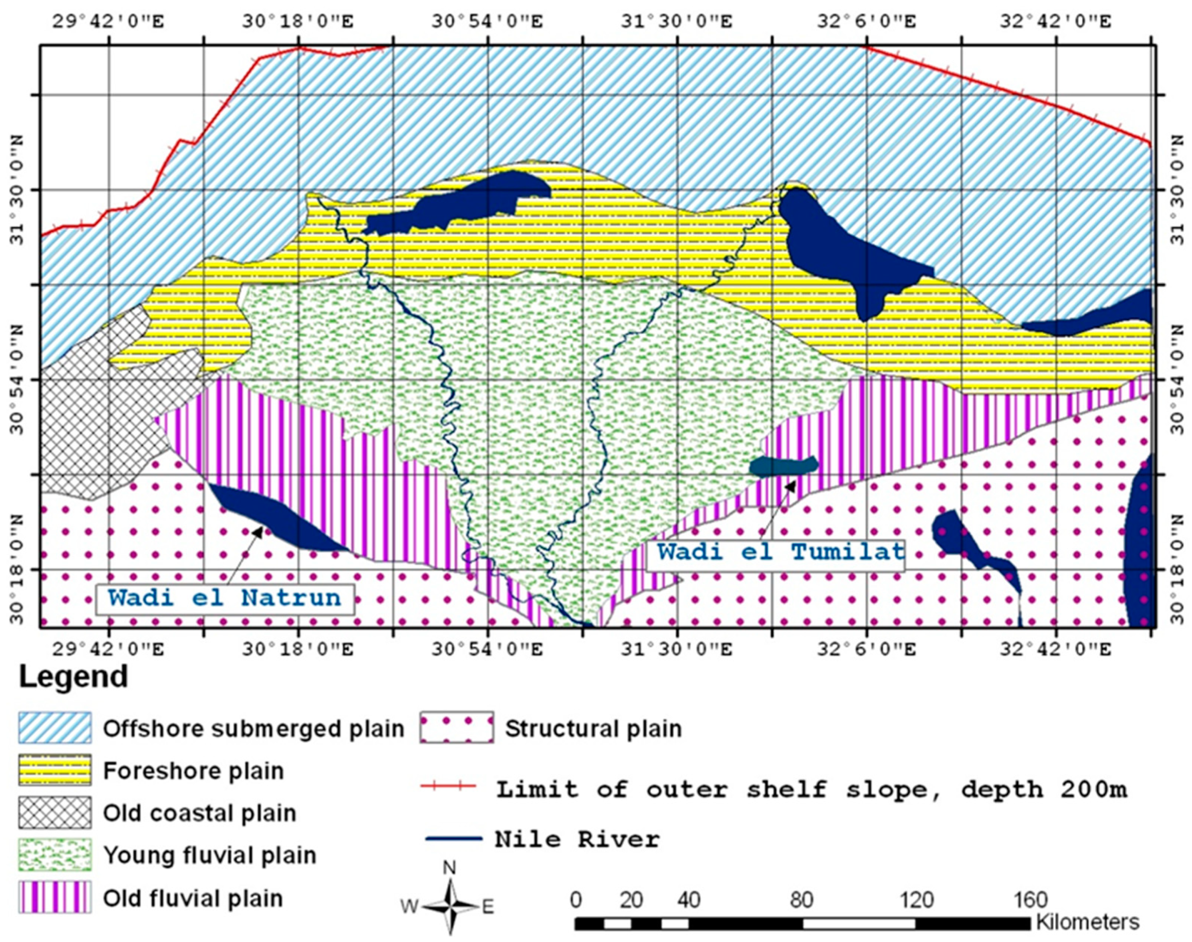
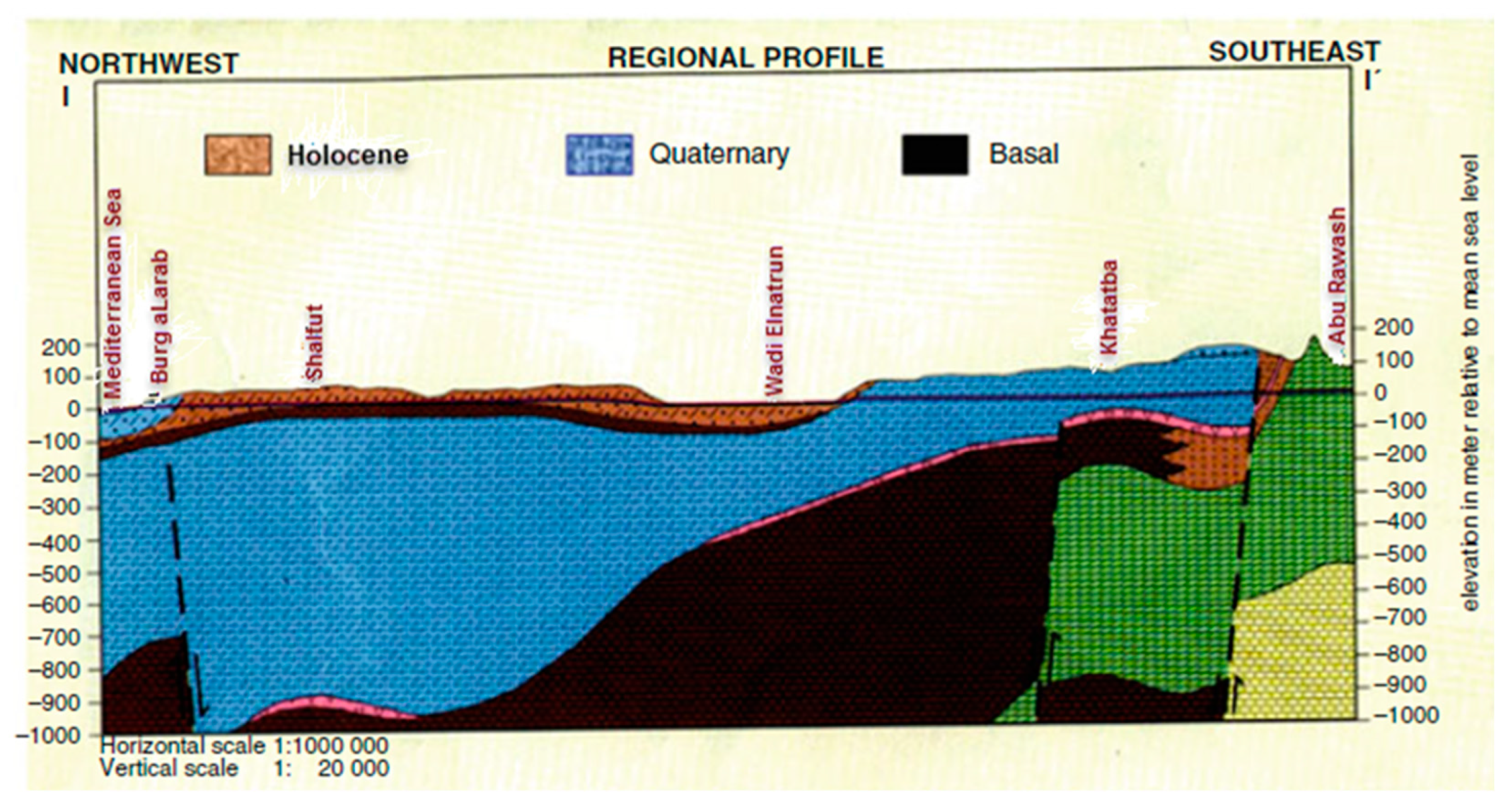
2.4. Geology of the Study Area

Two main geological components in the ND region are Quaternary deposits and Tertiary deposits. The Quaternary includes the Holocene and Pleistocene sediments. Holocene deposits are widely spread with maximum thickness of about 77 m [32]. Moreover, the thickness of Quaternary deposits increases in a northward direction to reach 250 m at the south and 1000 m at the north [33]. The Tertiary deposits including Pliocene, Miocene, Oligocene, Eocene and Paleocene sediments. El Shazly et al. [34] revealed that the lower Pliocene sediments are fluvio-marine and sandy clays. This forms the lower boundary of the Quaternary deposits. The hydrogeological cross section in the ND area is shown in Figure 2 [4].

The Quaternary aquifer contains coarse sand and gravel with occasionally clay lenses and underlies the Holocene top clay layer. The aquifer thickness increases northward, where the thickness ranges between 150 m in the south and more than 500 m near Tanta to 1000 m near the coast zone. Hydraulic conductivity of these layers increases northward and eastward and ranges between 50 m/day in the South to more than 100 m/day at the northward [35]. The Drainage Research Institute (DRI) [36] reported that the downward leakage towards the aquifer varies from 0.25 to 0.80 mm/day. The abstraction rates for drinking and irrigation purposes were 3.03 and 4.90 Billion Cubic Meter (BCM) per year in 1992 and 2008 respectively [37]. The depth of groundwater table in this aquifer ranges between 1 and 2 m at the North, 3–4 m at the Middle, and 5 m at the South [37,38].

2.5. Hydrogeology of the Study Area

The two Nile branches, Damietta and Rosetta are the main water resources in the ND. The ND consists of complex irrigation and drainage network, which are hydraulically connected to the aquifer system [25]. This area has a semi-confined Quaternary aquifer which covered by semi pervious clay and silt which acts as a cap for the main Quaternary aquifer [37]. The clay layer thickness varies from 5 to 20 m in the south and the middle and reaches to 50 m in the North [39]. Research Institute for Groundwater (RIGW) [37] estimated the average hydraulic conductivity of the clay cap is 2.5 mm/day in vertical direction and ranges between 50 and 500 mm/day in horizontal direction.

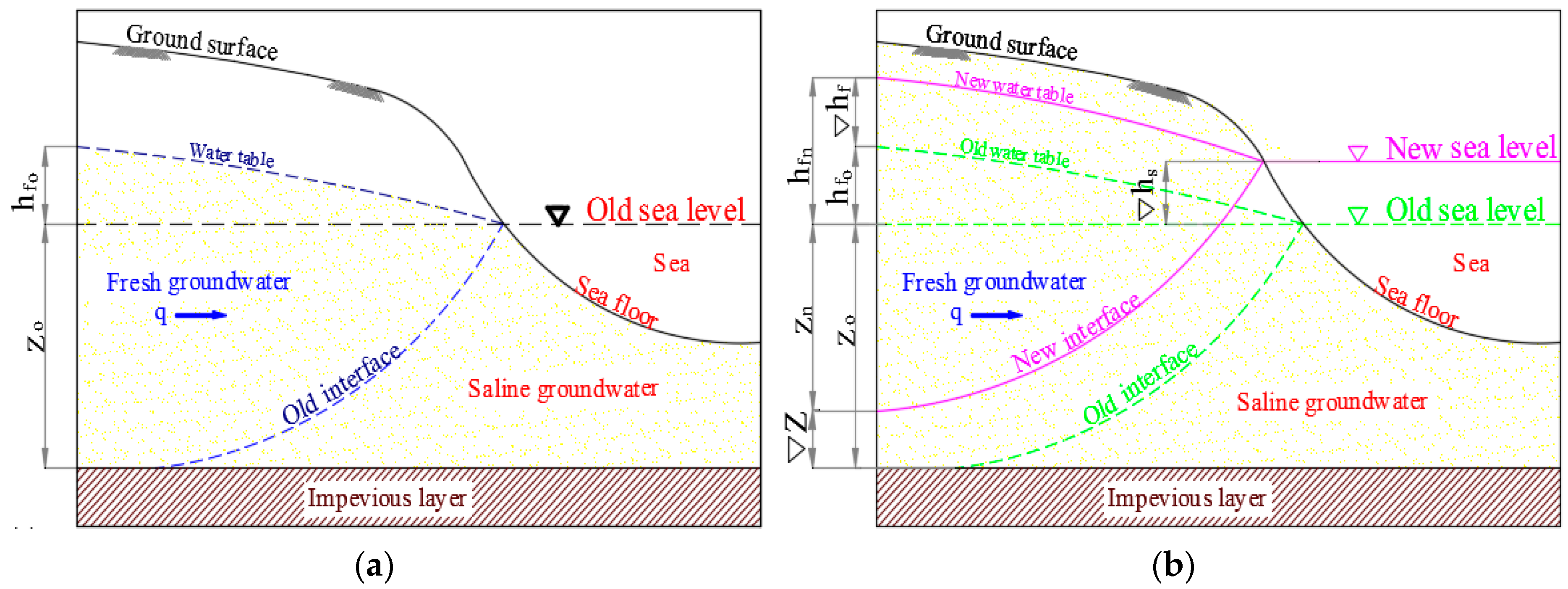
3. Analytical Solution of SWI in Coastal Aquifers

Analytical models simulate groundwater flow and contaminant transport for simple physical settings and low accuracy of model predictions [40]. Limitations of analytical models including flexibility of modeling are limited due to simplifying assumptions including isotropy, homogeneity, geometry, and simple initial conditions [41]. The hydrodynamic balance between freshwater and saltwater depends on shape and movement of mixing zone between the two fluids. Saltwater/freshwater interface bodies normally consist of narrow mixing zone. This interface in an intruded aquifer represents a flow line, which implies no flow across the surface [4].

The first model for SWI was developed by Ghyben [42] and Herzberg [43] which known as Ghyben-Herzberg model. This simple model draws the sharp saltwater/freshwater interface due to the hydrostatic equilibrium between the two immiscible fluids that having different densities of freshwater and saline water as shown in Figure 3a. The derived formula that discovered by Ghyben-Herzberg is based on an average value of fresh water and saline water densities (ρ_f = 1000 and ρ_s = 1025 kg/m³) can be written as:

$${\mathrm{Z}}_{\mathrm{o}}=\left(\frac{{\mathsf{\rho }}_{\mathrm{f}}}{{\mathsf{\rho }}_{\mathrm{s}}-{\mathsf{\rho }}_{\mathrm{f}}}\right){\mathrm{h}}_{\mathrm{f}}=\mathrm{G}\times {\mathrm{h}}_{\mathrm{f}}=40\times {\mathrm{h}}_{\mathrm{f}}$$

(1)

Muskat [44] studied the dynamics of saltwater interfaces and indicated that the pressure continuity in the flow field must be retained across the assumed interface. The interface governing equation based on potential function (head) for each fluid under equilibrium conditions, when saltwater is static or when both fluids are in motion can be written as following:

$${\mathrm{Z}}_{\mathrm{o}}=\left(\frac{{\mathsf{\rho }}_{\mathrm{f}}}{{\mathsf{\rho }}_{\mathrm{s}}-{\mathsf{\rho }}_{\mathrm{f}}}\right){\mathrm{h}}_{\mathrm{s}}-\left(\frac{{\mathsf{\rho }}_{\mathrm{f}}}{{\mathsf{\rho }}_{\mathrm{s}}-{\mathsf{\rho }}_{\mathrm{f}}}\right){\mathrm{h}}_{\mathrm{f}}$$

(2)

where:

Z₀ is the initial depth, ρ_s is the saline water density (MT⁻³), ρ_f is the freshwater density (MT⁻³), h_s is the depth of interface below mean sea level [L]; h_f is the height of the potentiometric surface above the mean sea level (L); G = ρ_f/(ρ_s − ρ_f) ≈ 40 for ordinary saltwater.

A number of analytical models were developed to estimate the saltwater/freshwater interface under different hydrological conditions based on theory of Hubbert as a foundation and with accurate field description between the two immiscible fluids behavior in coastal aquifers [4]. Glover [45] developed the movement and discharge of freshwater toward the sea for sharp interface in coastal aquifers. Also, it was found that freshwater flows through a thin gap between freshwater/saltwater interfaces and water table outcrops at the coast when dynamic factors are considered [4].

Cooper [5], indicated that in practice, saltwater/freshwater interface is not sharp (immiscible fluids) and the saline water merges gradually with the freshwater by mixing process uses the advection-dispersion equation (miscible fluids), also the study showed the water particles movement due to tides or variation due to recharge could affect the width of the dispersion zone [5]. Henry [46] developed the first semi-analytical solution based on Cooper’s hypothesis considering the mixing process including the effect of dispersion and density differences on seawater encroachment in confined coastal aquifer. Bower et al. [47] presented an analytical solution for saltwater upcoming in a leaky confined aquifer. The model assumed the existence of sharp interface between freshwater and saltwater.

In the current study a new equation is developed to investigate the freshwater/saline water interface based on Ghyben-Herzberg, considering the changes in boundary conditions (see Figure 3b). Equation (6) is used to calculate the shift in the saline of sharp interface (ΔZ) based on the difference in density between the fresh water and saline water (G), the freshwater difference (Δh_f) and the changes in sea level (Δh_s). The equation has been derived as following:

$${\mathrm{Z}}_{\mathrm{n}}=\left(\frac{{\mathsf{\rho }}_{\mathrm{f}}}{{\mathsf{\rho }}_{\mathrm{s}}-{\mathsf{\rho }}_{\mathrm{f}}}\right){\mathrm{h}}_{\mathrm{fn}}-\left(\frac{{\mathsf{\rho }}_{\mathrm{f}}}{{\mathsf{\rho }}_{\mathrm{s}}-{\mathsf{\rho }}_{\mathrm{f}}}\right){\mathsf{\Delta }\mathrm{h}}_{\mathrm{s}}$$

(3)

$${\mathrm{Z}}_{\mathrm{n}}-{\mathrm{Z}}_{\mathrm{o}}=\left(\frac{{\mathsf{\rho }}_{\mathrm{f}}}{{\mathsf{\rho }}_{\mathrm{s}}-{\mathsf{\rho }}_{\mathrm{f}}}\right){\mathrm{h}}_{\mathrm{fn}}-\left(\frac{\mathsf{\rho }\mathrm{s}}{\mathsf{\rho }\mathrm{s}-{\mathsf{\rho }}_{\mathrm{f}}}\right){\mathsf{\Delta }\mathrm{h}}_{\mathrm{s}}-\left(\frac{{\mathsf{\rho }}_{\mathrm{f}}}{{\mathsf{\rho }}_{\mathrm{f}}-{\mathsf{\rho }}_{\mathrm{f}}}\right){\mathrm{h}}_{\mathrm{fo}}$$

(4)

$$\mathsf{\Delta }\mathrm{Z}=\left(\frac{{\mathsf{\rho }}_{\mathrm{f}}}{{\mathsf{\rho }}_{\mathrm{s}}-{\mathsf{\rho }}_{\mathrm{f}}}\right)\left({\mathrm{h}}_{\mathrm{fn}}-{\mathrm{h}}_{\mathrm{fo}}\right)-\left(\frac{{\mathsf{\rho }}_{\mathrm{s}}}{{\mathsf{\rho }}_{\mathrm{s}}-{\mathsf{\rho }}_{\mathrm{f}}}\right){\mathsf{\Delta }\mathrm{h}}_{\mathrm{s}}$$

(5)

$$\mathsf{\Delta }\mathrm{Z}=\pm \mathrm{G}\times {\mathsf{\Delta }\mathrm{h}}_{\mathrm{f}}-\left(\mathrm{G}+1\right){\mathsf{\Delta }\mathrm{h}}_{\mathrm{s}}$$

(6)

where:

Z₀ is the initial depth of freshwater to sea water interface (L), Z_n is the new depth of fresh water to sea water interface (L), ΔZ is the difference in depth of fresh water to sea water interface (L), h_fo is the initial height of the potentiometric surface above the mean sea level (L), h_fn is the new height of the potentiometric surface above the mean sea level (L), Δh_fn is the difference height of the potentiometric surface above the mean sea level (L) it is positive for groundwater head above mean sea level (MSL) and negative where the groundwater level below MSL, Δh_s is the difference height of the sea level (L).

4. Numerical Simulation of Groundwater Flow and Solute Transport in MNDA

Visual MODFLOW (USGS, USA) is applied to simulate and investigate the groundwater flow in the MNDA. The study area is divided to 172 rows and 157 columns with cell area (1 km²) as presented in Figure 4a. The model is divided into 11 layer, the first layer is clay cap with depth ranged from 20 to 50 m and layers from 2 to 11 are divided into equal thickness. Two sections in X direction and Y direction are presented in Figure 4b,c.

4.1. Model Boundary Conditions

The study area boundary conditions are assigned by a constant head with zero value at the shoreline of the Mediterranean Sea. Also, in the two Nile branches, in Damietta branch the head ranged from 13.66 m at the south to 0.50 m at the north. However, in Rosita, branch the head ranged from 13.17 m at the south to 0.50 m at the north. The canals were assigned using river packages where the river head ranged from 16.17 m at south to 0.50 m at north above MSL. Also, drains were assigned using drain packages where the head ranged from 8 at South to 0.25 m at North above MSL, as shown in Figure 4.

4.2. Model Hydraulic Parameters

The hydraulic parameters of Nile Delta (ND) aquifer are shown in

Table 1. Hydrogeological parameters of the ND aquifer.

Main Hydraulic Units	Layer No	Hydraulic Conductivity		Storage Coefficient	Specific Yield	Effective Porosity
		Kh	Kv	Ss	Sy	n
		(m/day)	(m/day)	(-)	(-)	%
Clay	1	0.10–0.25	0.01–0.025	10−3	0.10	50–60
Fins Sand with Lenses of Clay	2, 3, 4 and 5	5–20	0.5–2	5 × 10−3	0.15	30
Course Sand Quaternary	6, 7, 8 and 9	20–75	2–7.50	2.50 × 10−3	0.18	25
Graded Sand and Gravel	10 and 11	75–100	7.50–10	5 × 10−4	0.20	20

which are used as input to the model. The parameters include hydraulic conductivity in horizontal direction (K_h) and vertical direction (K_v), specific storage (S_s), specific yield (S_y), and total porosity (n). These data collected from previous studies and some calculations [37]. The total abstraction in the study area is about 0.81×10⁹ m³/year in 2008 while the net recharge ranged from 0.20 to 0.80 mm per day [37]. A value of 250 m is used for the longitudinal dispersivity (α_L) while the lateral dispersivity (α_T) and the vertical dispersivity (α_V) are set equal to 25 m and 2.50 m, respectively. The diffusion coefficient is set equal to 10⁻⁴ m²/day [28].

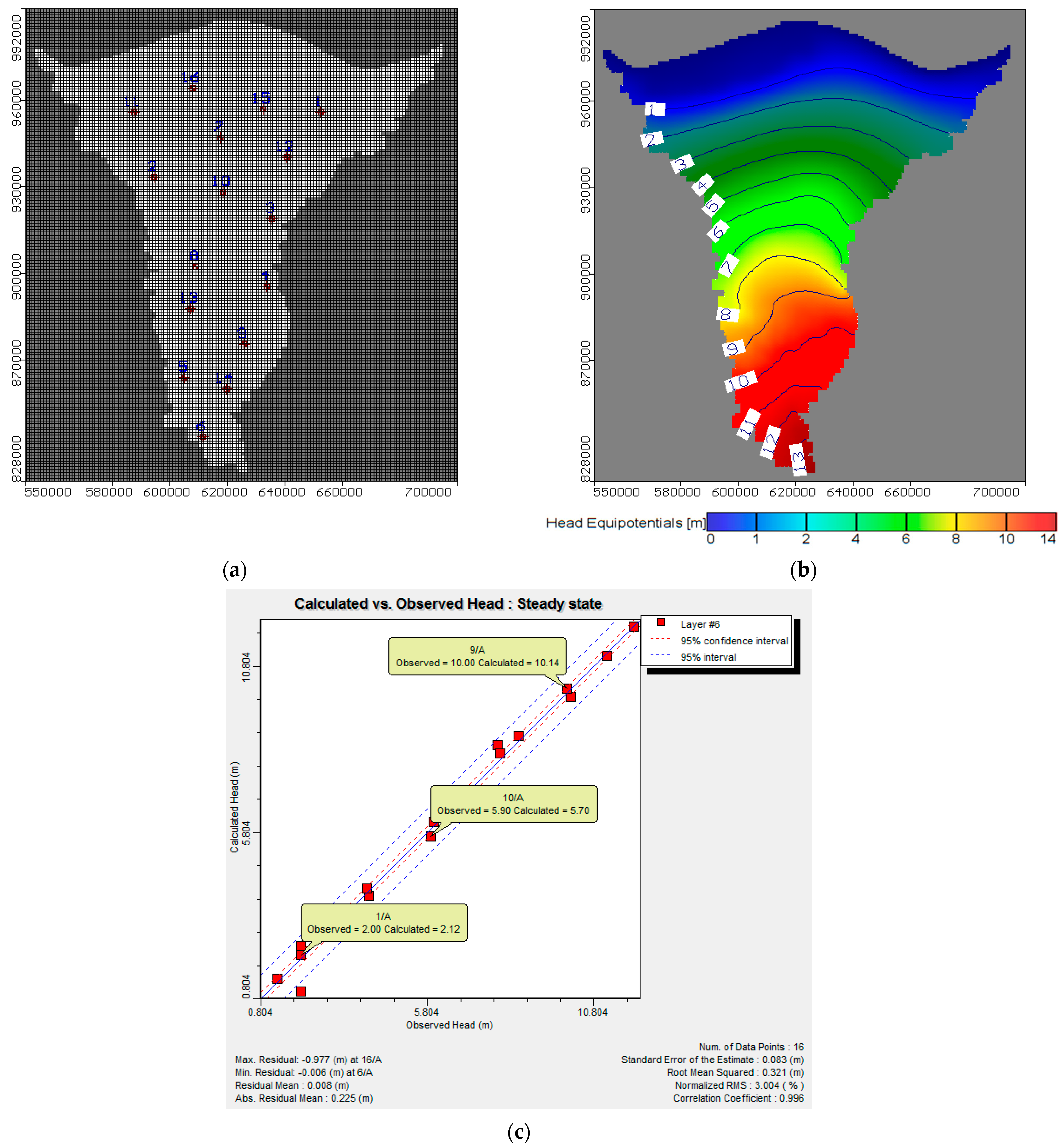
4.3. Model Calibration

SEWAT is used to simulate groundwater heads in the MNDA. Figure 5a presents the distribution of observation wells in the study area; also Figure 5b presents the distribution of groundwater flow in the aquifer at layer 2, where the flow direction changes gradually from high level at the south to low level along the shoreline of the Mediterranean Sea. The model calibration is done by trial and error to match between the field and calculated data. A number of 16 observation wells are used in the current simulation and the calibration results show that the residual varied between −0.006 and −0.977 m with root mean square (RMS) of 0.321 m and a normalization root mean square of 3.004% as shown in Figure 5c. The model was applied to predict groundwater flow under different scenarios. The predicted heads are used to calculate saltwater intrusion interface using the analytical solution. Then the model is used to assess the changes in groundwater heads in the MND aquifer due to different scenarios shown in

Table 2. Proposed scenarios for different years.

Scenario		Year
		2010	2070
1	Seal level rise (cm)	0	52.80
2	Reduction in Nile flow (%)	0	−18.50
	Nile flow (Billion m3/year)	55.50	45.20
	Recharge reduction for study area (Million m3/year)	5,935,800	4,837,677
3	Population increasing (%)	0	184%
	Egypt population (Million)	79	225
	50% of population increasing (%)	0	92%
	Abstraction of study area (Million m3/year)	2,220,414	4,263,195

.

The solute transport model is calibrated by comparing the results with other models which was developed to simulate the current study area. The model results have been compared with the numerical models developed by [12,48,49] where good agreement was obtained between the results. Also, the SEAWAT results showed that the equi-concentration line 1000 ppm and 35,000 ppm reached to 101.66 and 63.80 km, respectively, as presented in Figure 5b and Figure 6a. The calibrated results of this case for both groundwater head and salinity distribution in the MNDA are used as a base case for further scenarios.

5. Results

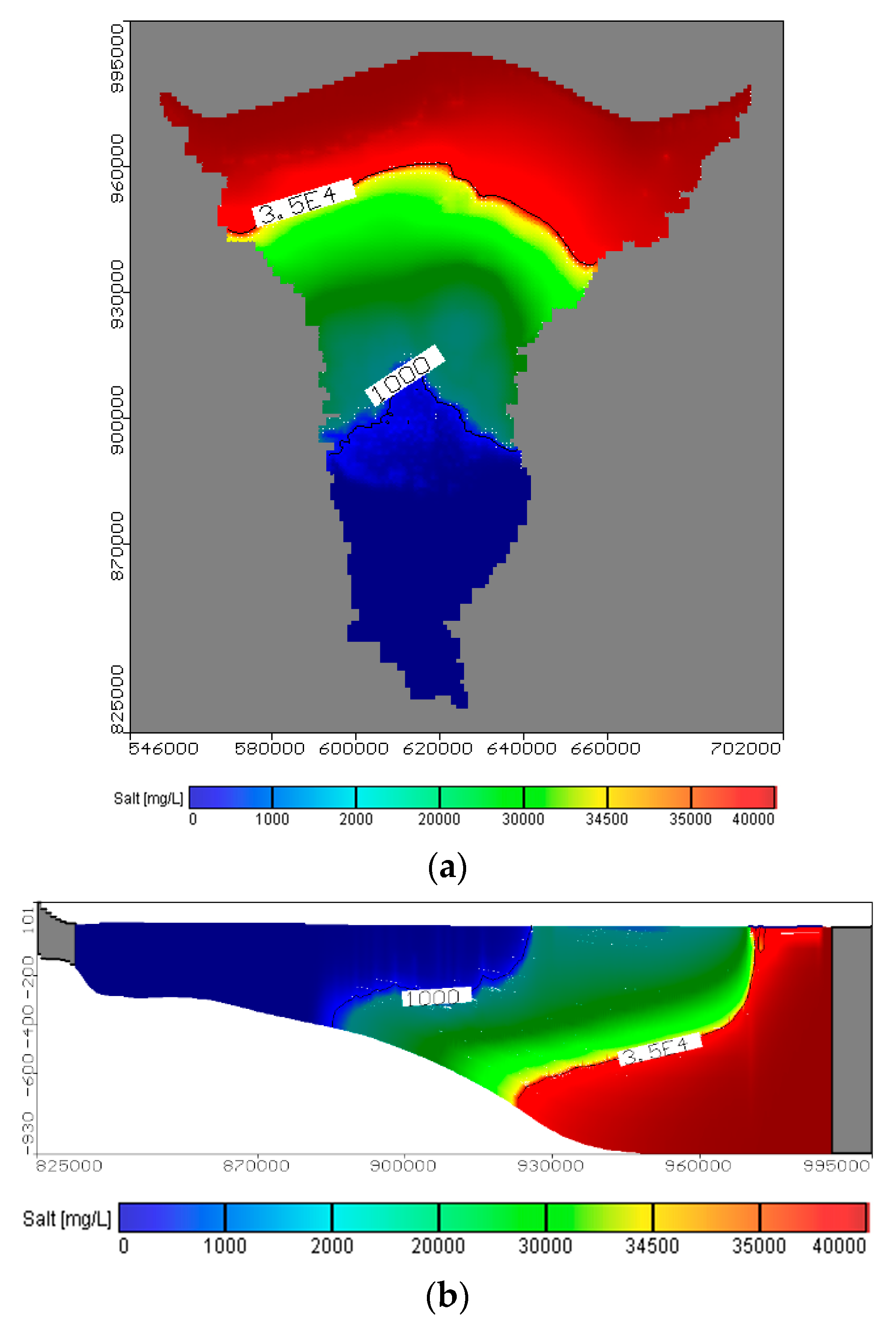
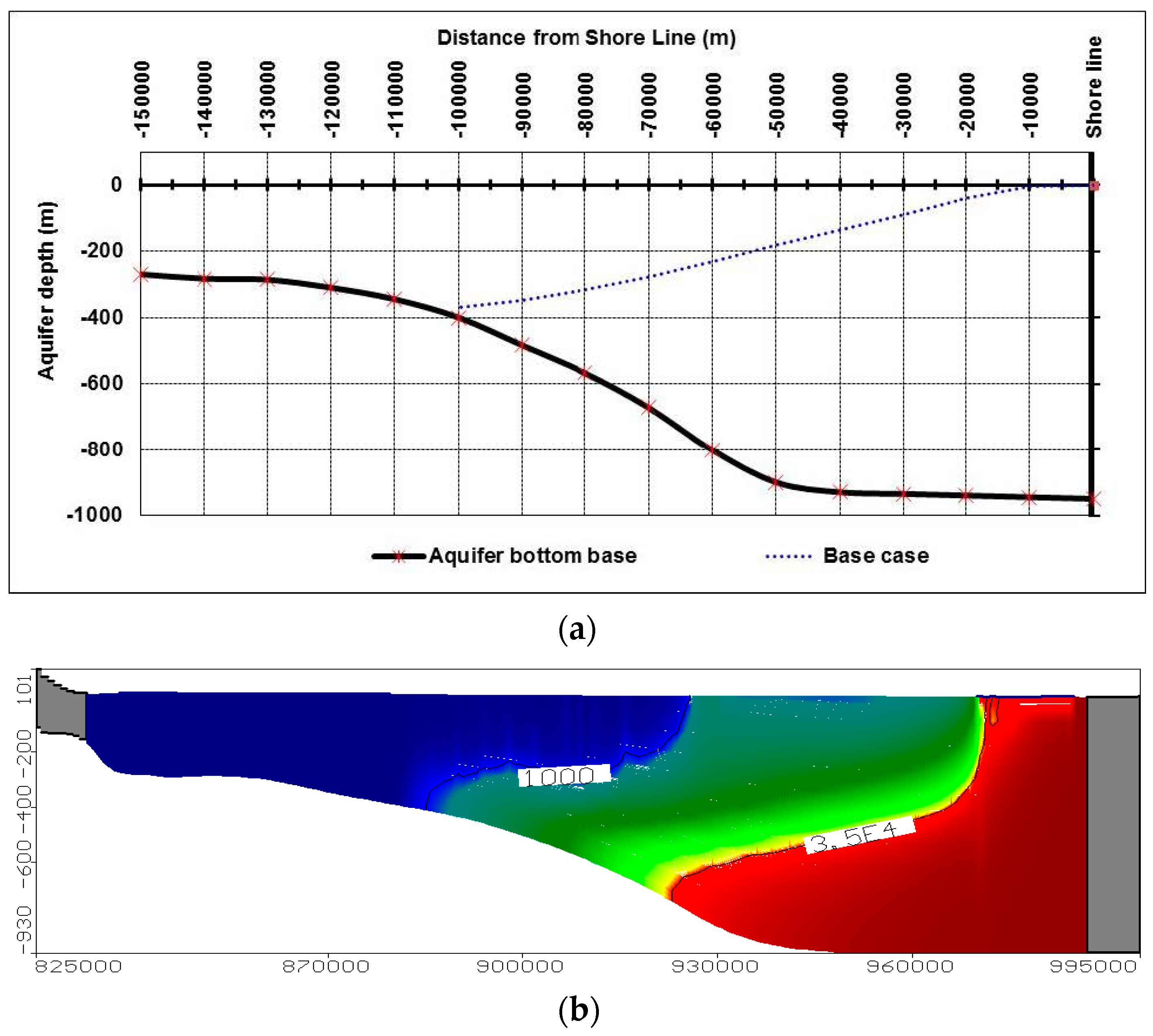
5.1. Simulation of Groundwater Flow in the MNDA

After model has been calibrated, the numerical model has been applied to simulate groundwater flow in the MNDA. Four scenarios are considered in this study to simulate groundwater flow. The first scenario is increasing the sea level by 52.80 cm at 2070 due to climate changes. The results showed that SLR has increased the groundwater head to reach 52.80 cm above the mean sea level (MSL) at the shoreline as presented in Figure 7. The second scenario is reducing groundwater recharge due to the reduction in the Nile flow by 18.50%. The groundwater head is decreased, and the maximum reduction has reached to 7.4 m above (MSL) at a distance of 100 km from shoreline due to the reduction in aquifer recharge (see Figure 7). The third scenario is increasing the groundwater abstraction by 92% at 2070 due to the expected increase in population. The results showed that over pumping has decreased the head to reach 5.2 m above MSL at 100 km from shoreline for the maximum reduction in water levels (see Figure 7). The fourth scenarios are combination of three scenarios; rise 52.80 cm in SLR, reduction in Nile flow by 18.50% and increase in abstraction by 92%. The results showed that this scenario has a greater reduction in groundwater head at the middle part of the ND which reached to 3.3 m above (MSL) at distance 100 km from shoreline (see Figure 7).

5.2. Simulation of SWI in the MNDA Using Numerical and Anylatical Models

The analytical model is used to determine the vertical distribution of TDS by calculating the difference in depth of freshwater to sea water interface (ΔZ) using Equation (6) and shift the initial depth of freshwater to seawater interface (Z_o) by this value to determine the new depth of fresh water to saline water interface (Z_n). SWI distribution in the aquifer has been predicted using the analytical solution as presented in Figure 8a. Also, numerical model (SEWAT) is used to simulate the same case and the results are presented in Figure 8b. The results of both models showed that equiconcentration line 1 moved to a distance of 103 and 101.66 km from the seaside in analytical and numerical models, respectively. The results gave good agreement between numerical and analytical model for the base case as shown in Figure 8a,b. Then, both models have been used to simulate SWI in the MNDA considering four scenarios after 50 years (2070) as described in the following sections.

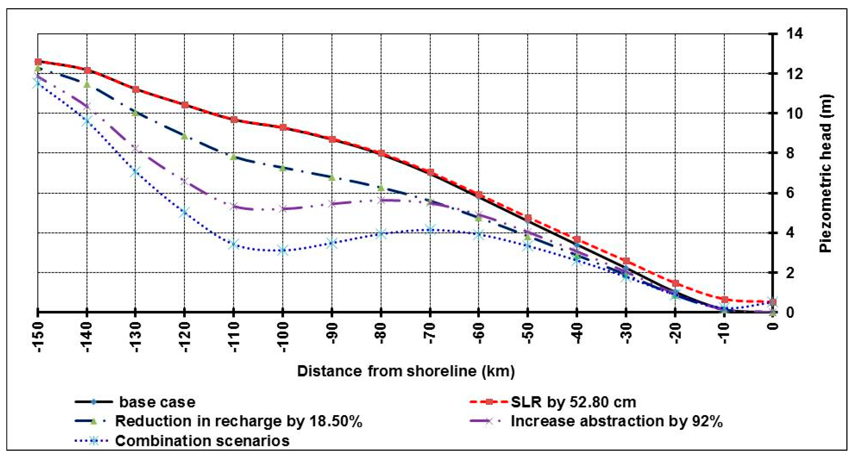
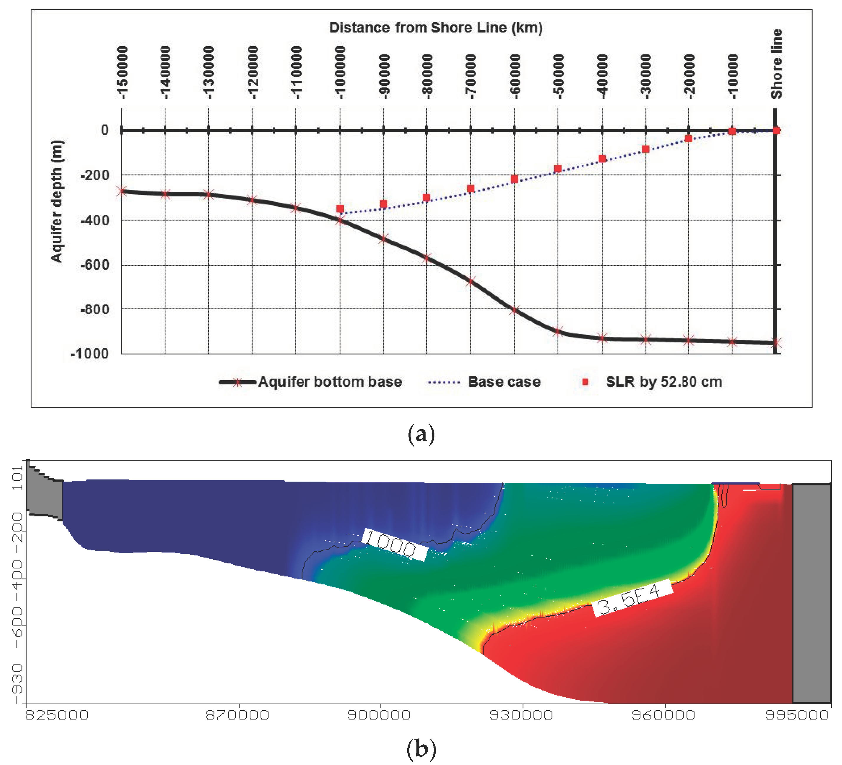
5.2.1. Impact of SLR on SWI in the MNDA

In this scenario an increase in the sea level by 52.80 cm at 2070 due to climate changes has been applied. The results showed that SLR has increased the intrusion length in both analytical and numerical models. A new position of the equi-concentration line 1 was detected in land direction. SWI was predicted and the intrusion changed with small values from the shoreline due to increasing the seawater level where intrusion reached 105 km in analytical model and 103.45 km for numerical model. Also, equiconcentration line 35 reached 65.03 km for the numerical model. The results showed that the two models’ results are very close, as shown in Figure 9a,b.

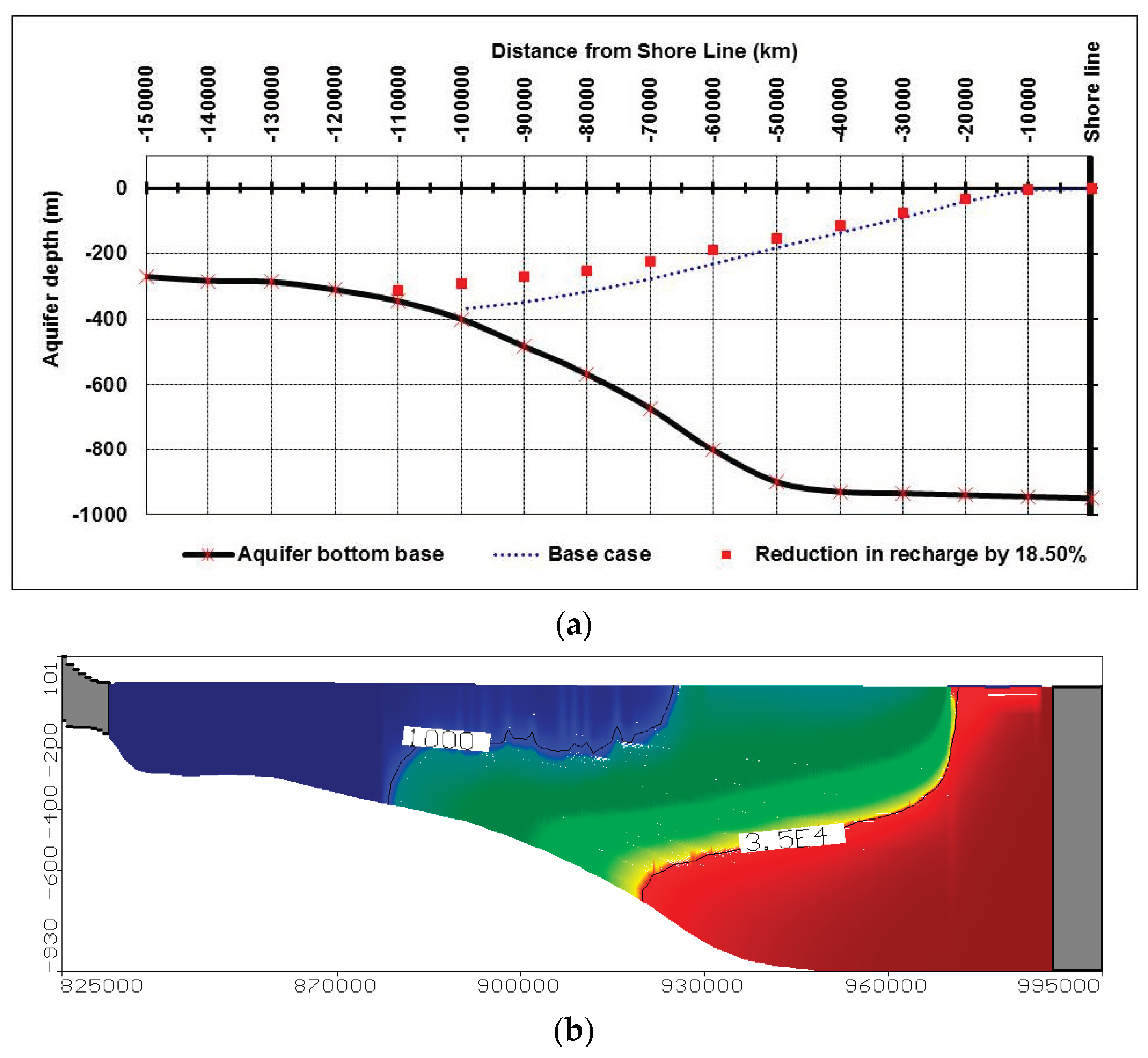
5.2.2. Impact of Decreasing the Nile Flow on SWI in the MNDA

The analytical and numerical models have been applied to study the reduction in Nile flow on SWI in the MNDA by 18.50% from base case. The intrusion of equiconcentration line 1 for analytical model reached 111 km and 108.25 km from shoreline for numerical model as presented in Figure 10a,b. The intrusion reached 66.90 km for the equiconcentration line 35 by the numerical model.

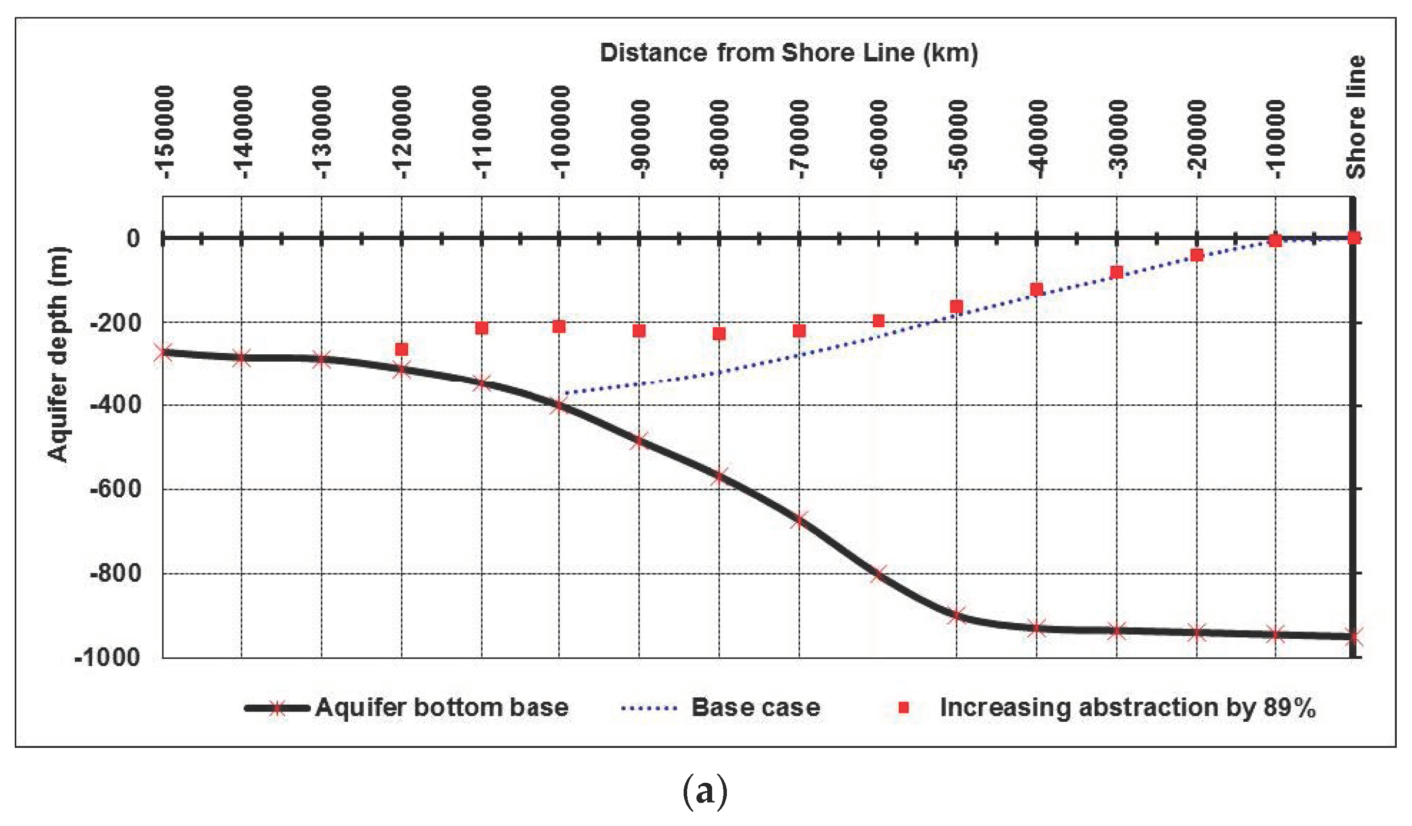
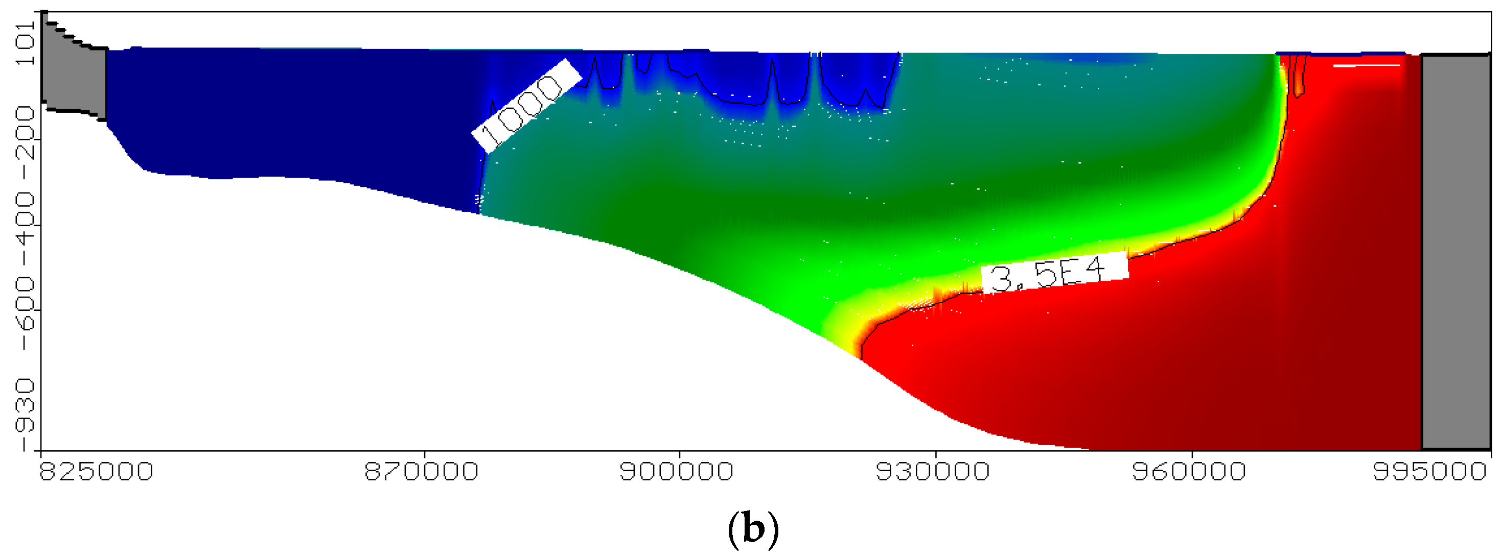
5.2.3. Impact of over Abstraction on SWI in the MNDA

In this scenario the abstraction from the aquifer has increased to 92% after 50 years (2070) from base case due to increase in population. The intrusion length of equiconcentration line 1 reached 121 km and 110.30 km from shoreline for analytical and numerical models respectively as shown in Figure 11a,b. The intrusion reached 65.33 km for equiconcentration line 35 in the numerical model. The difference between the two models is due to that over pumping abstracted saline water in the numerical model and the intrusion rates is decreased to reach 65.33 km at this case compared to 66.90 km at reduction in recharge.

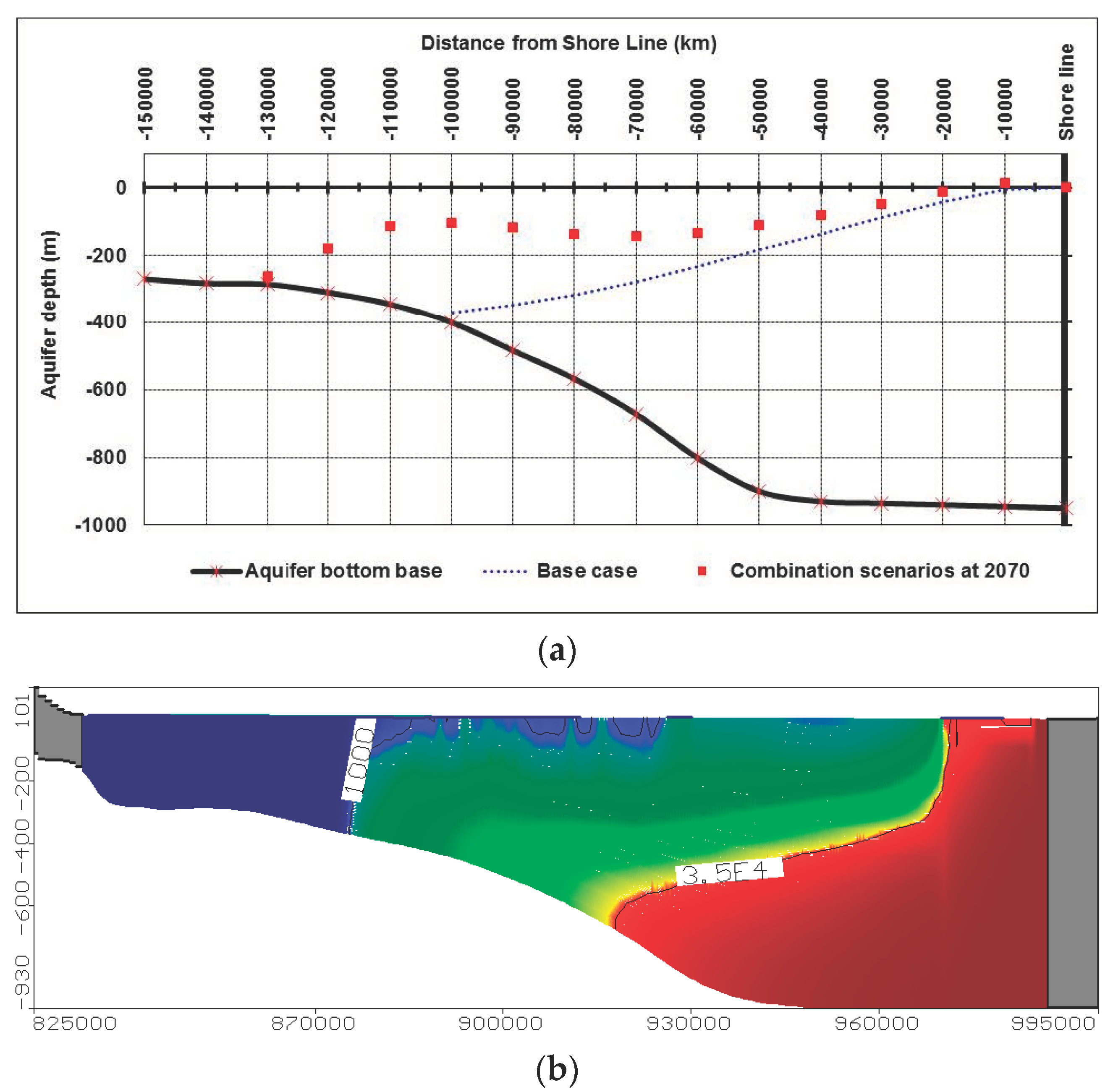
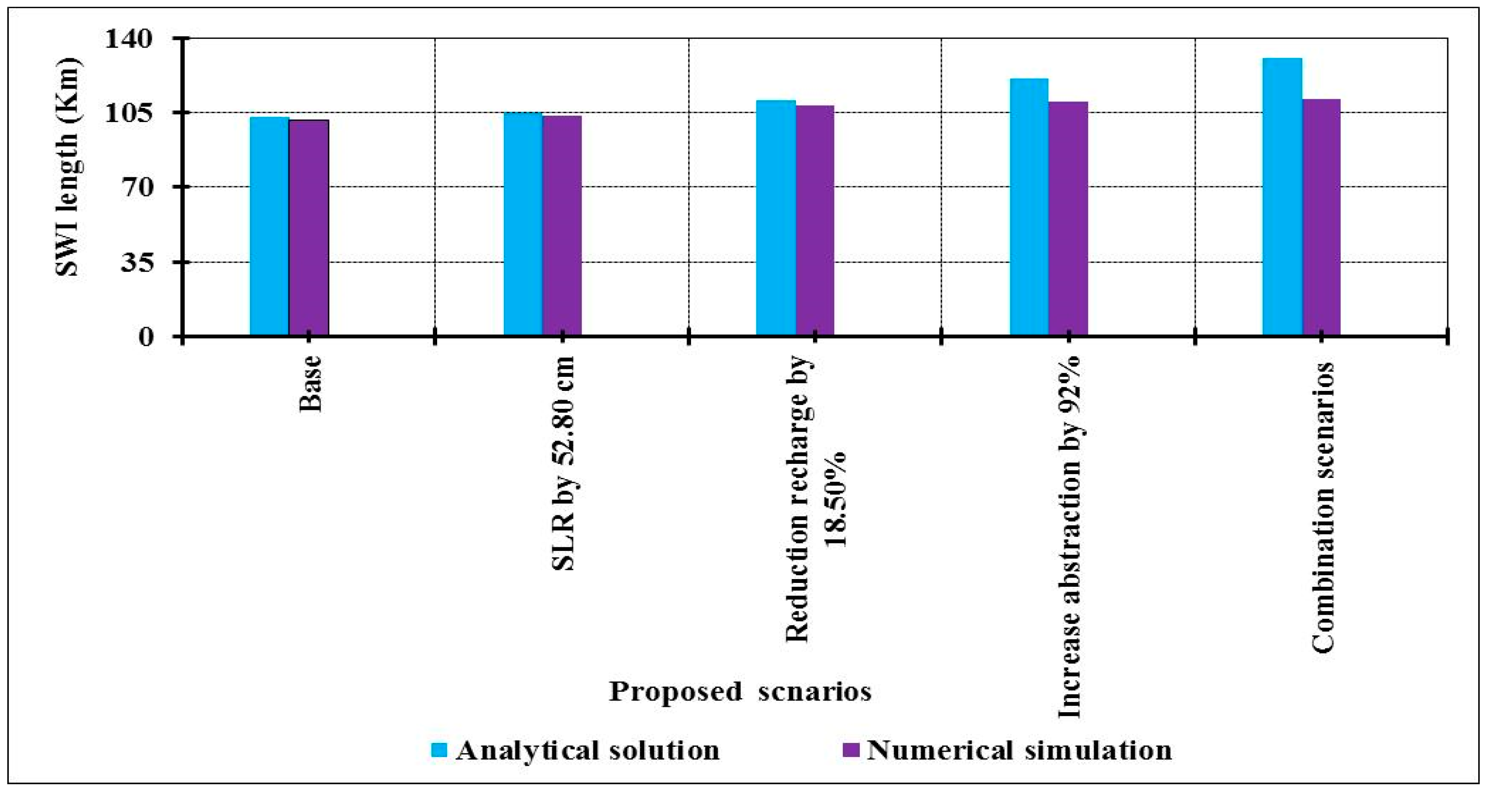
5.2.4. Impact of Combination of Scenarios 1, 2 and 3 on SWI in the MNDA

This scenario presents the combination of the previous three scenarios; SLR, decrease in Nile flow and increasing the abstraction rates from the ND aquifer. In this case, the intrusion length of equiconcentration line reached 131 km for analytical solution and 111.66 km for numerical solution respectively as shown in Figure 12a,b. The equi-concentration line 35 reached 68.94 km in the numerical model. The higher intrusion in the analytical solution is due to neglecting the abstraction force for saltwater compared with the numerical solution considering over pumping.

6. Discussion

In this study analytical model and numerical model (SEAWAT) have been used to simulate groundwater flow and solute transport in coastal aquifers and then applied to a real case study at the MNDA. SEAWAT code is used to simulate groundwater flow in the MNDA considering four scenarios. The sea level by 52.80 cm has increased the groundwater head to reach 52.80 m above MSL at shoreline. The reduction in the Nile flow by 18.50% decreased the head to 7.4 m above (MSL) at distance 100 km from shoreline. The increase of groundwater abstraction by 92% decreased the head to reach 5.2 m above MSL at 100 km from shoreline. However, the combination of the three scenarios resulted in more reduction in groundwater head in the middle part of Nile delta to reach 3.3 m above (MSL) at distance 100 km from shoreline.

Then both numerical and analytical models applied to simulate salinity distribution in the MNDA considering different scenarios. The results of all scenarios for both analytical and numerical models are presented in

Table 3. Intrusion length of Equiline 1 for analytical and numerical model.

Scenario			Analytical Model	Numerical Model	The Differences (%)(XTA − XTN)/XTA
No	Case	Value	Intrusion Length (km)	Intrusion Length (km)
			Equiline 1	Equiline 1	Equiline 1
1	base	-	103	101.66	1.30
2	Seal level rise (cm)	52.80	105	103.45	1.48
3	Reduction in Nile flow (%)	−18.50	111	108.25	2.48
4	Over pumping	92%	121	110.31	8.84
5	Combination of scenario1, 2 and 3	Combination of values in 1, 2 and 3	131	111.32	15.02

. Figure 13 shows a comparison between results for equi-concentration 1 from numerical and analytical models for different scenarios in 2070. The results of the base case for the two models gave a good agreement where the intrusion reached to 103 and 101.66 km measured at the base of the aquifer for the analytical and numerical solution respectively. The increase in sea levels by 52.80 cm at 2070 increased the intrusion in the two models where the SWI reached 105 and 103.45 km for analytical and numerical models respectively. Also, the reduction in recharge by 18.50% increased the intrusion for the two models where the SWI reached 111 and 108.25 km for analytical and numerical solution respectively. Over pumping has increased the intrusion to reach 121, 110.31 km for the two models while the combination of the three scenarios increased the intrusion to reach 131 and 111.32 km for analytical and numerical models respectively.

The difference percentage between the analytical and numerical models for different scenarios has been determined using the following relation:

The differences (%) = (XT_A − XT_N)/XT_A

(7)

where, XT_A is the intrusion length for the analytical solution and XT_N is the intrusion length for numerical solution.

The calculated percentage for the base case and the four scenarios are 1.30%, 1.48%, 2.48%, 8.84%, and 15.02%, respectively, as presented in Table 3. From the results a good agreement obtained between the two models in most of the cases. The results revealed that the analytical model is capable of simulating such large cases studies with high accuracy.

The main limitation of this study was the lack of updated data for such case studies which was addressed by the authors through some field data and literature review.

7. Conclusions

Saltwater intrusion into coastal aquifers could have a great effect on freshwater quality in these aquifers. Analytical and numerical models could be used to simulate SWI in such cases. In the current study, analytical and numerical models are developed to simulate groundwater flow and saltwater intrusion in the MNDA. This aquifer is subject to changes in boundary condition due to rise in sea level, changes in freshwater heads in landside due to reduction in recharge, increase in the abstraction rates and decrease in the Nile flow. The analytical and numerical models are used to simulate SWI in the study area considering different scenarios including; sea level rise, reduction in the Nile flow, over abstraction, and combination scenarios after 50 years (2070). The groundwater heads were predicted using Visual MODFLOW to be used in the analytical solution to determine SWI for different scenarios. In this study a new formula is developed to determine the changes in freshwater/saline water interface due to changes in boundary conditions. The analytical results compared with the numerical. The result with the base case is very close in the two models, where the intrusion for equiconcentration lines 1 reached to 103 and 101.66 km for the two models, respectively. Also, the investigated intrusion at 2070 and equiconcentration lines 1 reached 105, 111, 121, and 131 km in the analytical solution and 101.66, 103.45, 108.25, 110.31, and 111.32 km in the numerical simulation for the four scenarios including; sea level rise by 52.80, reduction in Nile flow by 18.50% cm due to the expected climate changes, increasing in abstraction by 89% due to over population and combination scenarios. The developed analytical model for the current real case study gave good results compared with the numerical model as the difference between the two solutions reached to 1.30%, 1.48%, 2.48%, 8.84%, and 15.02% for the base case and the future four scenarios considered in this study. The analytical solution is recommended for similar studies which save time and capabilities of computers required in the numerical solutions.

References

1. Cheng, A.H.-D.; Benhachmi, M.K.; Halhal, D.; Ouazar, D.; Naji, A.; Harrouni, K.E. Pumping optimization in saltwater-intruded aquifers. In Coastal Aquifer Management: Monitoring, Modeling and Case Studies; Cheng, A.H.-D., Ouazar, D., Eds.; CRC Press: Boca Raton, FL, USA, 2004; pp. 178–197. [Google Scholar]
2. Narayan, K.A.; Schleeberger, C.; Charlesworth, P.B.; Bistrow, K.L. Effects of groundwater pumping on saltwater intrusion in the lower Burdekin Delta, North Queensland. In MODSIM 2003 International Congress on Modelling and Simulation; Post, D.A., Ed.; Modelling and Simulation Society of Australia and New Zealand: Perth, Australia, 2003; pp. 212–217. [Google Scholar]
3. Sreekanth, J.; Datta, B. Multi-objective management of saltwater intrusion in coastal aquifers using genetic programming and modular neural network based surrogate models. J. Hydrol. 2010, 393, 245–256. [Google Scholar] [CrossRef]
4. Sakr, S.A. Impact of the Possible Sea Level Rise on the Nile Delta Aquifer. A Study for Lake Nasser Flood and Drought Control Project (LNFDC/ICC); Planning Sector, Ministry of Water Resources and Irrigation: Cairo, Efypt, 2005.
5. Cooper, H.H. A hypothesis concerning the dynamic balance of fresh water and saltwater in a coastal aquifer. J. Geophys. Res. 1959, 64, 461–467. [Google Scholar] [CrossRef]
6. IPCC. Annex B: Glossary of terms. In Climate Change 2001: Impacts, Adaptation and Vulnerability; McCarthy, J.J., Canziani, O.F., Eds.; Cambridge University Press: Cambridge, UK, 2001; p. 995. [Google Scholar]
7. Klein, M.; Lichter, M. Statistical analysis of recent Mediterranean Sea-level data. Geomorphology 2009, 107, 3–9. [Google Scholar] [CrossRef]
8. IPCC. Summary for policy makers. In Climate Change 2014: Impacts, Adaptation, and Vulnerability. Synthesis Report based on the Contribution of the three Working Groups to the Fifth Assessment Report of the Intergovernmental Panel on Climate Change; Field, C.B., Barros, V.R., Eds.; Cambridge University Press: Cambridge, UK, 2014; pp. 1–32. [Google Scholar]
9. Werner, A.D.; Simmons, C.T. Impact of sea-level rise on seawater intrusion in coastal aquifers. Groundwater 2009, 47, 197–204. [Google Scholar] [CrossRef] [PubMed]
10. Abd-Elhamid, H.F.; Javadi, A.A. Impact of Sea Level Rise and Over-pumping on Seawater Intrusion in Coastal Aquifers. J. Water Clim. Chang. 2011, 2, 19–28. [Google Scholar] [CrossRef]
11. Abd-Elhamid, H.F.; Javadi, A.A.; Qahman, K. Impact of over-pumping and sea level rise on seawater intrusion in Gaza aquifer. J. Water Clim. Chang. 2015, 5, 222–234. [Google Scholar] [CrossRef]
12. Abd-Elhamid, H.; Javadi, A.; Abdelaty, I.; Sherif, M. Simulation of seawater intrusion in the Nile Delta aquifer under the conditions of climate change. J. Hydrol. Res. 2016, 47, 1–14. [Google Scholar] [CrossRef]
13. Wassef, R.; Schüttrumpf, H. Impact of sea level rise on groundwate rsalinity at the development area western delta, Egypt. Groundw. Sustain. Dev. 2016, 2, 85–103. [Google Scholar] [CrossRef]
14. Sbai, M.A.; Larabi, A.; De Smedt, F. Modelling saltwater intrusion by a 3- D sharp interface finite element model. WIT Trans. Ecol. Environ. 1998, 17, 1743–3541. [Google Scholar]
15. Marin, L.E.; Perry, E.C.; Essaid, H.I.; Steinich, B. Hydrogeological investigations and numerical simulation of groundwater flow in karstic aquifer of northwestern Yucatan, Mexico. In Proceedings of the 1st International Conference and Workshop on Saltwater Intrusion and Coastal Aquifers, Monitoring, Modelling, and Management, Essaouira, Morocco, 23–25 April 2001. [Google Scholar]
16. Barnett, B.; Townley, L.R.; Post, V.; Evans, R.E.; Hunt, R.J.; Peeters, L.; Richardson, S.; Werner, A.D.; Knapton, A.; Boronkay, A. Australian Groundwater Modelling Guidelines; National Water Commission: Canberra, Australia, 2012. [Google Scholar]
17. Abd-Elhamid, H.F. A Simulation-Optimization Model to Study the Control of Seawater Intrusion in Coastal Aquifers. Ph.D. Thesis, College of Engineering, Mathematics and Physical Sciences, University of Exeter, Exter, UK, December 2010. [Google Scholar]
18. Todd, D.K. Salt-water intrusion and its control. Water technology/resources. J. Am. Water Work. Assoc. 1974, 66, 180–187. [Google Scholar] [CrossRef]
19. Sakr, S.A. Three-Dimensional Finite Element Model of Seawater Intrusion in Aquifers. Ph.D. Thesis, Faculty of Engineering, Colorado State University, Fort Collins, CO, USA, 1995. [Google Scholar]
20. EEAA. Egypt Second National Communication under the United Nations Framework Convention on Climate Change (UNFCCC); Egyptian Environmental Affairs Agency, Ministry of State for Environmental Affairs: Cairo, Egypt, 2010.
21. RIGW. Hydrogeological Map of Nile Delta, Scale 1:500,000, 1st ed.; RIGW: Kanater El Khairia, Nile Delta, Egypt, 1992.
22. WMRI-NWRC. Unpublished Report under the Matching Supply and Demand Project; Water Management Research Institute, National Water Research Center, Ministry of Water Resources and Irrigation: Cairo, Egypt, 2002.
23. Farid, M.S. Management of Groundwater System in the Nile Delta. Ph.D. Thesis, Cairo University, Cairo, Egypt, 1985. [Google Scholar]
24. Shata, A.; El-Fayoumey, I. Remarks on the regional geological structure of the Nile Delta. Proceeding of the Bucharest Symposium on Hydrogeology of Deltas, Bucharest, Romania, 6–14 May 1969; pp. 189–197. [Google Scholar]
25. MWRI. Adaptation to Climate Change in the Nile Delta through Integrated Coastal Zone Management; Ministry of Water Resources and Irrigation: Cairo, Egypt, 2013.
26. Agrawala, S.; Annett, M.; El Raey, M.; Declan, C.; Maarten van, A.; Marca, H.; Joel, S. Development and Climate Change in Egypt: Focus on Coastal resources and the Nile; Environment Policy Committee, Working Party on Global and Structural Policies and Working Party on Development Co-operation and Environment; Organization for Economic Co-operation and Development (OECD): Paris, France, 2004. [Google Scholar]
27. Coastal Research Institute (CORI). Studying Shoreline Changes along El Burullus Coastal Zone, Nile Delta Coast during the Period (2004–2014); Technical Report; Coastal Research Institute (CORI): Los Angeles, CA, USA, 2015. [Google Scholar]
28. Sherif, M.M.; Sefelnasr, A.; Javad, A. Incorporating the concept of equivalent freshwater head in successive horizontal simulations of seawater intrusion in the Nile Delta aquifer, Egypt. Hydrogeol. J. 2012, 464, 186–198. [Google Scholar] [CrossRef]
29. Abd-Elhamid, H.F.; Abd-elaty, I.; Sherif, M. Evaluation of on Seawater Intrusion in the Nile Delta Aquifer potential impact of Grand Ethiopian Renaissance Dam. Int. J. Environ. Sci. Technol. 2018, 16, 2321–2332. [Google Scholar] [CrossRef]
30. Sayed, M.A.; Nour El-Din, M.M.; Nasr, F.M. Impacts of Global Warming on Precipitation Patterns on the Nile Basin. In Proceedings of the Second Regional Conference on Action Plans for Integrated Development, Cairo, Egypt, 12–15 April 2004. [Google Scholar]
31. Strzepek, K.; Yates, D.; Yohe, G.; Tol, R.; Mader, N. Constructing not implausible Climate and Economicscenarios for Egypt. Integr. Assess. 2001, 2, 139–157. [Google Scholar] [CrossRef]
32. Zaghloul, Z.M.; Taha, A.A.; Hegab, O.; El Fawal, F. The Neogene’s Quaternary Sedimentation Basins of the Nile Delta. Egypt. J. Geol. 1977, 21, 1–48. [Google Scholar]
33. El-Fayoumy, I.F. Geology of Groundwater Supplies in the Eastern Region of the Nile Delta and its Extension in North Sinai. Ph.D. Thesis, Faculty of Science, Cairo University, Cairo, Egypt, 1968; pp. 1–207. [Google Scholar]
34. El Shazly, E.M. Geological and Groundwater Potential Studies of Ismailia Master Plane Study Area. Remote Sensing Research Project; Academy of Scientific Research and Technology: Cairo, Egypt, 1975; pp. 1–24. [Google Scholar]
35. RIGW (Research Institute for Groundwater). Projected of the Safe Yield Study for Groundwater Aquifer in the Nile Delta and Upper Egypt. Part1; Ministry of Irrigation, Academy of Scientific Research and Technology, and Organization of atomic Energy: Cairo, Egypt, 1980. (In Arabic)
36. DRI. Mashtul Pilot Area, Physical Description; Technical Report No. 57, Pilot Areas and Drainage Technology Project; Drainage Research Institute: El-Qanater El-Khiriaya, Egypt, 1987. [Google Scholar]
37. Morsy, W.S. Environmental Management to Groundwater Resources for Nile Delta Region. Ph.D. Thesis, Faculty of Engineering, Cairo University, Cairo, Egypt, 2009. [Google Scholar]
38. RIGW. Nile Delta Groundwater Modeling Report; Research Institute for Groundwater: Kanater El-Khairia, Egypt, 2002.
39. Diab, M.S.; Dahab, K.; El Fakharany, M. Impacts of the paleohydrological conditions on the groundwater quality in the northern part of Nile Delta, The geological society of Egypt. Geol. J. B 1997, 4112, 779–795. [Google Scholar]
40. Wels, C.; Mackie, D.; Scibek, J. Guidelines for Groundwater Modelling to Asses Impacts of Proposed Natural Resource Development Activities; Technical report; Report n 194001; British Columbia Minstry of Environment—Water Protection and Sustainability Branch: Victoria, BC, Canada, 2012.
41. Kumar, C.P. Groundwater Flow Models; National Institute of Hydrology: Roorkee, India, 2002. [Google Scholar]
42. Ghyben, B.W. Nota in Verband Met de Voorgenomen put Boring Nabij Amsterdam; Tydscrift Van Het Koninkyky Institute Van Ingenieurs: Hague, The Netherlands, 1889; p. 21. [Google Scholar]
43. Herzberg, A. Die wasserversorgung Einnger Nordsecbader. JGUW 1901, 44, 815–819. [Google Scholar]
44. Muskat, M. The Flow of Homogeneous Fluids Through Porous Media; McGraw-Hill: New York, NY, USA, 1937. [Google Scholar]
45. Glover, R.E. The pattern of freshwater flow in a coastal aquifer. J. Geophys. Res. 1959, 64, 457–459. [Google Scholar] [CrossRef]
46. Henry, H. Effects of dispersion on salt encroachment in coastal aquifer. U.S. Geol. Surv. Water Supply Pap. 1964, 1613, 70–84. [Google Scholar]
47. Bower, J.W.; Motez, L.H.; Durden, D.W. Analytical Solution for the Critical Conditions of Saltwater Upconing in a Leaky Artesian Aquifer. J. Hydrol. 1999, 221, 43–54. [Google Scholar] [CrossRef]
48. Abdelaty, I.M.; Abd-Elhamid H., F.; Fahmy, M.R.; Abdelaal, G.M. Study of Impact Climate Change and Other on Groundwater System in Nile Delta Aquifer. EIJEST 2014, 17, 2061–2079. [Google Scholar]
49. Nofal, E.R.; Amer, M.A.; El-Didy, S.M.; Fekry, A.M. Delineation and modeling of seawater intrusion into the Nile Delta Aquifer: A new perspective. Water Sci. 2015, 29, 156–166. [Google Scholar] [CrossRef] [Green Version]
Figure 1. Configuration of aquifer systems at the Nile delta region [4].
Water 13 00995 g001
Figure 2. Hydrogeological cross section in the Nile Delta area [4].
Water 13 00995 g002
Figure 3. Schematic diagram of freshwater-saltwater interface position for (a) Freshwater-saltwater interface position (Ghyben-Herzberg) (b) Freshwater-saltwater interface position for incremental changes in the boundary condition.
Water 13 00995 g003
Figure 4. Model domain discretization and boundary conditions for the MNDA (a) Areal view, (b) Cross section in X-direction, (c) Cross section in Y-direction.
Water 13 00995 g004
Figure 5. Calibration and results of groundwater flow model in MNDA (a) distribution of observation wells, (b) Areal view of groundwater head in MND aquifer, (c) Model calibration for calculated versus observed heads.
Water 13 00995 g005
Figure 6. Salinity distribution in the MNDA using the numerical model. (a) Areal view, (b) Vertical cross section.
Water 13 00995 g006
Figure 7. Future GWH at different scenarios of SLR, Nile flow rates, abstraction rates and combination of the three scenarios.
Water 13 00995 g007
Figure 8. Current SWI distribution in the MNDA (base case) (a) Analytical solution (b) Numerical solution.
Water 13 00995 g008
Figure 9. SWI distribution in the MNDA due to SLR (a) Analytical solution (b) Numerical solution.
Water 13 00995 g009
Figure 10. SWI distribution in the MNDA due reduction in recharge. (a) Analytical solution, (b) Numerical solution.
Water 13 00995 g010
Figure 11. SWI distribution in the MNDA due increasing abstraction rates. (a) Analytical solution, (b) Numerical solution.
Water 13 00995 g011aWater 13 00995 g011b
Figure 12. SWI distribution in the MNDA due to combination of three scenarios. (a) Analytical solution, (b) Numerical solution.
Water 13 00995 g012
Figure 13. Comparison between results of numerical and analytical solution for different scenarios at 2070.
Water 13 00995 g013