
Evaluating the Structure from Motion Technique for Measurement of Bed Morphology in Physical Model Studies


1
Department of Civil and Environmental Engineering, Norwegian University of Science and Technology (NTNU), S.P. Andersens Veg 5, 7491 Trondheim, Norway
2
Hydro Lab Pvt. Ltd., GPO Box No 21093, Kathmandu 44600, Nepal
*
Author to whom correspondence should be addressed.
Water 2021, 13(7), 998; https://doi.org/10.3390/w13070998
Submission received: 2 March 2021
/
Revised: 25 March 2021
/
Accepted: 29 March 2021
/
Published: 5 April 2021
(This article belongs to the Special Issue Advances and Challenges in Hydropower)
Abstract
:The selection of instrumentation for data acquisition in physical model studies depends on type and resolution of data to be recorded, time frame of the model study, available instrumentation alternatives, availability of skilled personnel and overall budget of the model study. The available instrumentation for recording bed levels or three-dimensional information on geometry of a physical model range from simple manual gauges to sophisticated laser or acoustic sensors. In this study, Structure from Motion (SfM) technique was applied, on three physical model studies of different scales and study objectives, as a cheap, quicker, easy to use and satisfactorily precise alternative for recording 3D point data in form of colour coded dense point cloud representing the model geometry especially the river bed levels in the model. The accuracy of 3D point cloud generated with SfM technique were also assessed by comparing with data obtained from manual measurement using conventional surveying technique in the models and the results were found to be very promising.
1. Introduction
The use of physical hydraulic models to study different hydraulic phenomena has a history spanned over a few centuries. Since the fundamental theoretical background on producing hydraulically similar models were already put forward by past researchers, the advancement in physical hydraulic modelling since then were mostly focused on measurement, data acquisition and processing technologies. The laboratory instrumentation for physical hydraulic models have been evolved from simple manual gauges to highly sophisticated acoustic, ultrasonic and laser-based measurement systems [1]. However, various laboratories around the world still use the simple manual/mechanical instrumentation for measurements in physical hydraulic models because of their simplicity in operation as well as in data interpretation and their low logistical cost, though the measurement processes with those instruments are more time consuming. Whereas, relatively sophisticated thus expensive instrumentations are more accurate and less time consuming but require high logistical cost and specialized user expertise for data acquisition and analyses. These advanced measurement systems can be tailored for semi or fully automatic data acquisition curtailing the experiment time. However, the availability of instrumentation facilities, skills of the operator, time and budget for a given experiment ultimately govern the selection of measurement techniques for the experiment.
Traditional close-range digital photogrammetry was successfully used, in both field and laboratory measurements, as a cost-effective method to create 3D surface of a topography [2,3,4]. But the traditional photogrammetry is time consuming and the user is required to have a keen knowledge of mathematical foundations of photogrammetry in order to reconstruct an accurate 3D model [5]. When 3D laser scanning technology was released, it was supposed to completely replace the traditional photogrammetry, because of its accuracy and automation level [6]. But recent developments in photogrammetry and computer vision have made many improvements in the automated extraction of three-dimensional information from 2D images to generate accurate and dense models. Hence, image-based techniques are still widely used as the most complete, economical, portable and flexible method to generate 3D models [7]. Backed by complex algorithms, various commercial and open-source software are available to implement photogrammetric techniques, most of which can be used even by non-vision experts [8].
Structure from Motion (SfM) is a widely used photogrammetric technique which utilizes multi-view 3D reconstruction technology to produce high-resolution 3D models of a target object from a series of overlapping 2D images [9,10,11]. The fundamental advantage of SfM over traditional photogrammetry is its capability to automatically determine geometry of the target object, camera positions and orientation without prior need for a set of defined control points [9,12,13]. SfM solves these parameters simultaneously using a highly redundant, iterative bundle adjustment procedure based on a dataset of distinct features extracted automatically from the given set of images [14]. All the processes in SfM, from identification of key features to 3D reconstruction of scene geometry, can be automated which makes it more practical and cheaper alternative compared to traditional photogrammetry. SfM can be a low-cost but reliable alternative to other sophisticated measurement techniques also as it can be applied with images taken from low-cost consumer level digital cameras [9,15,16] or even from smartphones and complete processing can be carried out with freely available tools/software. With easy access to unmanned aerial vehicles (UAVs) and drones, which can be equipped with camera and sensors, SfM technique has also been widely used in medium to large-scale terrestrial surveying [17,18]. The accuracy of SfM for generation of high-resolution 3D topography has been validated by multiple studies [15,19,20] with some results being highly comparable to laser-based techniques [8,21,22].
The advantages of photogrammetric method over laser scanning are low operation cost, short data acquisition time, high quality of colour information and scalable 3D point clouds as output [23]. For example, Lane [3] spent about 8 h just to collect the data, using a laser sensor on a motorized cart, required to create a DEM with 0.5 mm resolution on a 0.25 m x 0.25 m area. To achieve the similar output using SfM technique, the required images can be acquired in few minutes and can be processed to produce 3D models within a couple of hours. Additionally, SfM technique is capable of producing better detailed 3D surface since images can be taken from various angles and distances unlike the laser-based measurements with limited measurement angles. The SfM technique has the potential to bridge the spatial scales between detailed measurement of small areas and coarser large-scale measurements [23]. However, SfM technique has some shortcomings like: majority of the users are not aware of the fundamental mathematics behind it; the accuracy of final output is hugely affected by lighting conditions during photography; difficulty in reproducing smooth or transparent surfaces with indistinct features/textures [22,24,25,26]. SfM technique have been widely applied in field-scale terrestrial surveying [27,28], geosciences [9,10,15,17,29], archaeology [30,31,32,33] and also in robotics [34,35,36], real estate and even in film productions. A few researchers have used it to study fluvial geomorphology in laboratory flumes and physical river models [3,37,38,39,40,41,42,43].
This study presents the evaluation of SfM technique in different model scale case studies to record 3-dimensional bed topography for different stages of tests and to quantify the extent and volume of change in riverbed topography in each case studies. In this study, images were acquired using handheld photography, instead of using camera installed in fixed orientation on moving trolleys, to reduce the logistical cost and image acquisition time. With handheld photography, it is also possible to put more focus on important details by taking images from different angles and distances specially in irregular shaped physical river models. The objective of this study is to evaluate the applicability of SfM technique with close range handheld photography in physical hydraulic model studies to capture 3D topography for each test event and to quantify the changes in riverbed topography. The applicability of SfM technique was evaluated by comparing the accuracy of 3D point clouds produced using SfM technique against the manual measurement data acquired using conventional surveying techniques.
2. Method
2.1. Ground Control Points (GCPs) and Georeferencing
The 3D model produced by SfM technique is created based on relative spatial relationships among locations of extracted feature points on multiple images taken from different viewpoints [19]. Therefore, the 3D model output preserves the shape of the target object but the size is arbitrarily scaled [44]. Hence, georeferencing of the 3D model output shall be done by transforming it to original scaling and coordinates in reference to a set of pre-defined ground control points (GCPs). The GCPs with known coordinates shall be marked on the model before capturing the images. The accuracy in defining these GCPs is crucial to avoid structural errors in resulting 3D models [15]. The structural errors are caused by erroneous scaling of the 3D model output in reference to the inaccurately defined control points. For better results, the GCPs should be distributed in such a way that it covers all the concerned area [45]. Micheletti [19] recommended to use at least 5 GCPs. The accuracy of output 3D model can be increased by increasing the number of GCPs [46] since the accuracy in reproducing elevations in 3D model output increases with decreasing distance to GCPs [47]. For better accuracy in 3D model output, each GCP should be visible in at least three images from different viewpoints [9]. It is recommended to define GCPs beforehand and then process the images for generating 3D model output in actual scaling and coordinates. However, it is also possible to produce a 3D model output in arbitrary scaling and coordinates and then transform it into original scaling and coordinates by using rotation, translation and scaling in reference to the GCPs. If the camera captures geotagged images, then the GCPs are not required but the accuracy of results may not be satisfactory for small scale objects [48]. Although scale river models were used in this study, the GCPs were defined with actual prototype coordinates to avoid ambiguities. Hence, the 3D model outputs were generated in original prototype scaling and coordinates.
2.2. Image Acquisition
A Sony α6300 (model ILCE-6300) camera was used for capturing images for the study. It was a mirrorless digital camera with 24-megapixel Exmor RS sensor and 425 phase detection autofocus points. For flexibility and time saving in image acquisition, the camera was operated in hand-held condition without using tripods or trolleys. Since handheld camera operation is prone to camera shaking at lower shutter speed resulting blurry images, the maximum exposure time (associated with slowest shutter speed) was kept below 1/100 s to avoid ‘motion blur’ effect in images due to camera shaking. The camera’s aperture was allowed to vary for optimum image exposure under the normal laboratory lighting condition, which resulted in camera aperture ranging from F9 to F11. The focal length of the camera lens was fixed at 16 mm. With these settings, the camera was operated in handheld condition to capture sets of overlapping images from varying viewpoints and orientations covering the whole study area. Additional closeup images of important features were taken from different angles to achieve better detailing.
2.3. Digital Photogrammetry
Nowadays various commercial and free software are available to cater the implementation of SfM technique in different applications. Based on the comparison among different SfM software made in [49], Agisoft Photoscan was selected for this study. Agisoft Photoscan (now available as Agisoft Metashape) is a commercial software developed by Agisoft LLC, Russia. It is a complete package loaded with all the capabilities from processing images to generating 3D models in form of a dense point cloud, a mesh and a Digital Elevation Model (DEM). It also includes additional pre-processing and post processing features. It is capable of processing both aerial and close-range photographs, and is efficient in both controlled and uncontrolled conditions. The software has a linear project-based workflow [8] consisting of: feature matching and aligning photographs; building dense point cloud; building mesh; generating texture; and exporting results [50]. In this study, dense point clouds and DEMs were generated with Photoscan. The quality of dense point clouds designated as Ultra high, High, Medium, Low and Lowest can be selected in Photoscan to specify the desired reconstruction quality. Mentioned quality settings were relative to the resolution of original input images and it provides the users to keep a balance between the quality of output and the processing time. In this study, we have used “medium” and “high” quality settings for different case studies. The DEMs were then exported to compute volume between two point-cloud surfaces using 2.5D volume computation tool in ‘CloudCompare’ software.
The total processing time is largely determined by specification of the workstation used and the extent of the study area. In this study, a workstation with Intel® Core™ i7-4790 CPU @3.60GHz processor, 32 GB RAM and 18 GB NVIDIA GeForce GTX 750 Ti GPU was used.
2.4. Manual Measurements
Manual measurements of a few cross-sections were also carried out in the physical models using a level machine, a staff gauge and a distance measuring bar with an accuracy of ±1 mm. These data were used for comparison with the corresponding cross-section profiles extracted from the 3D model outputs by SfM technique. In addition, a few distances between random pairs of the established GCPs were also measured manually to assess the accuracy of SfM output models.
3. Case Studies
3.1. Case Study I: Measurement of Changes in Bed Morphology
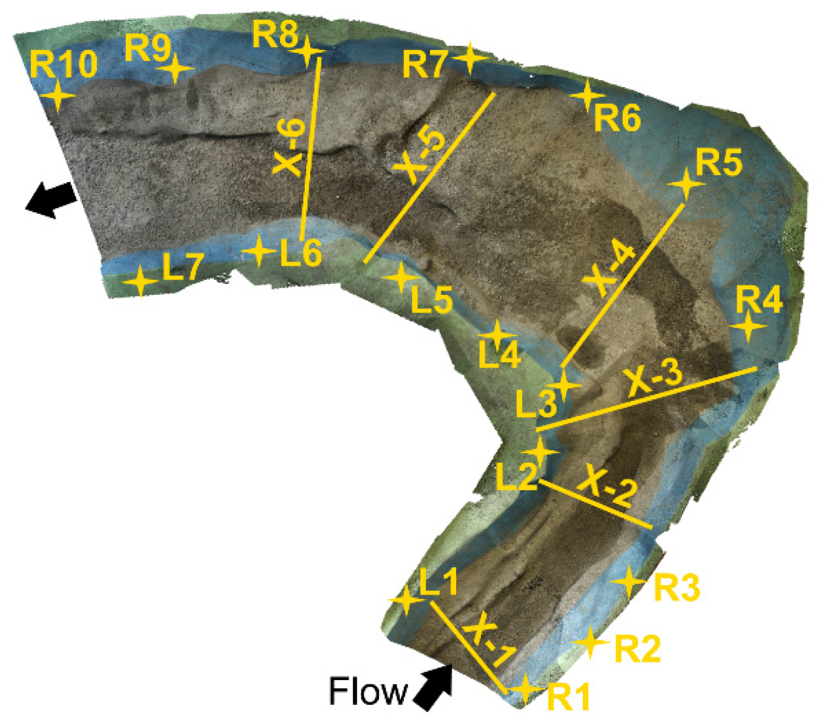
In case study I, the SfM technique was applied to record changes in bed morphology during a physical model study. The objective of the model study was to simulate evolution of river bed morphology during high sediment transport event and to create a database to validate a 1D numerical model developed for simulating river morphology in sediment laden rivers. The study was conducted on a physical hydraulic model representing 1 km long reach of Trishuli River in Nepal (Figure 1). Trishuli River is a typical Himalayan river with steep bed gradient which becomes relatively flatter after it crosses Betrawati. The selected river reach has an average bed slope of about 1:200 and consists of a sharp bend. The particular reach was chosen for the study since evolvement of river bed morphology is prominent in reaches with flatter bed gradient and with bends.
The 12.5 m long undistorted Froude scaled model at hydraulic laboratory of Hydro Lab in Nepal, representing the 1 km long reach of Trishuli river under study, was built in 1:80 scale. The modelled river channel had a fixed bed which was then filled with sand to provide a mobile bed having an average longitudinal slope of 1:200, in order to match the original bed slope in the prototype. The sand used for preparing mobile bed had median particle diameter (d50) of 0.55 mm, d90 of 1.28 mm and geometric standard deviation (σg) in particle size of 1.972. Similar sediment was also fed with inlet discharge during the simulation. It is to be noted that d50 of the prototype sediment is about 0.1 mm which shall be represented by model sediment with d50 = 1.25 microns to fulfill the scaling requirements for an undistorted Froude model. But using such a fine sediment in the model will introduce cohesion in the sediment particles and there is possibility of alteration of sediment transport phenomena from bed load in the prototype to suspended load in the model [51]. According to Bretschneider, the particle size of sand in models should be greater than 0.5 mm [52] to avoid the scale effects due to cohesion between sediment particles and changes in flow-grain interaction characteristics. Therefore, a model sediment having d50 = 0.55 mm was used in this study. A steady discharge of 40 L/s (2290 m3/s in prototype, which is close to the magnitude of 2 years return period flood) was supplied into the model with sediment feeding at the rate of 10 kg/min which corresponds to sediment concentration of 4167 ppm in the flow. The concentration of sediment fed into the model is about 5 times of average concentration for given discharge as estimated from the site measurement data. The experiment was run for 140 min (about 21 h in prototype) only. Due to high sediment concentration and the flatter river bed gradient, most of the sediment fed with inflow discharge deposited along the channel. The effect of the river bend was clearly visible with the flow concentrating towards the outer bank (the right bank) accompanied with small scour on the initially filled sediment bed while most of the sediment fed was deposited along inner bank (the left bank). A distinct delta front was witnessed propagating to downstream direction, which can be seen in Figure 2.
The river-bed topographies of initial bed and final river bed after simulation were recorded and respective 3D dense point clouds and DEMs were produced in prototype scale with actual coordinates (meters) and elevations (in masl) using SfM technique. The quality and size of the output dense point clouds and total processing time for each stage were given in Table 1.
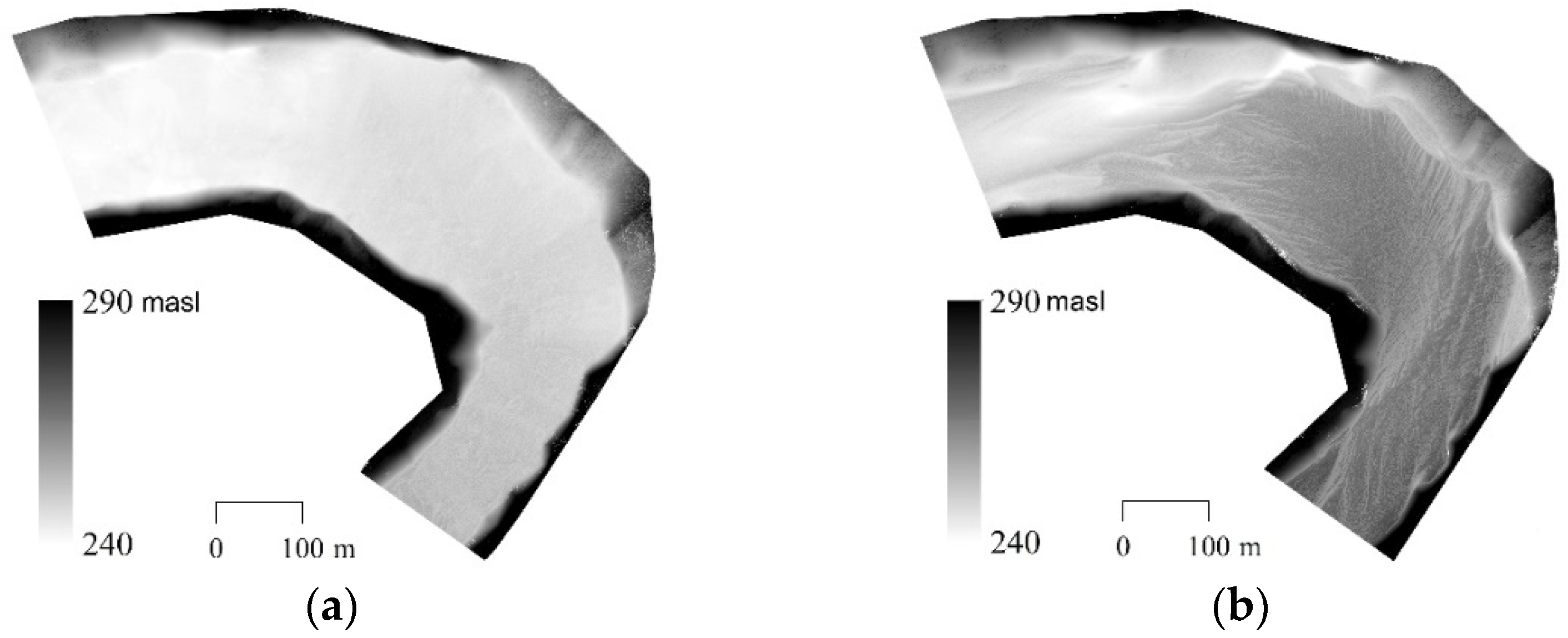
The DEMs of initial river bed and the river bed after test run are shown in Figure 2a,b respectively. Total 17 GCPs, 10 in the right bank (R1-R10) and 7 in the left bank (L1-L7), distributed over the study area (Figure 1) were used for georeferencing the 3D models into actual coordinates.
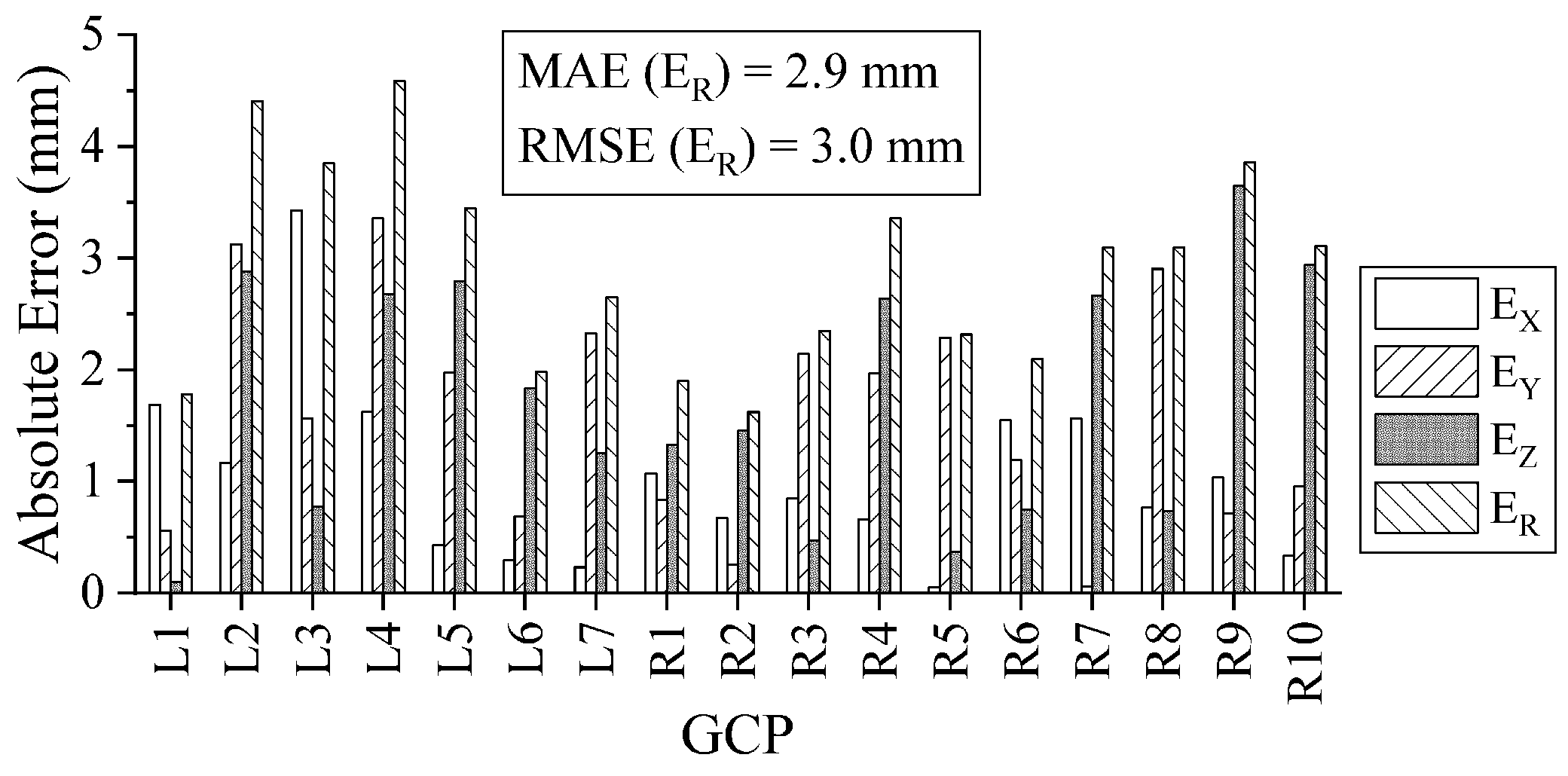
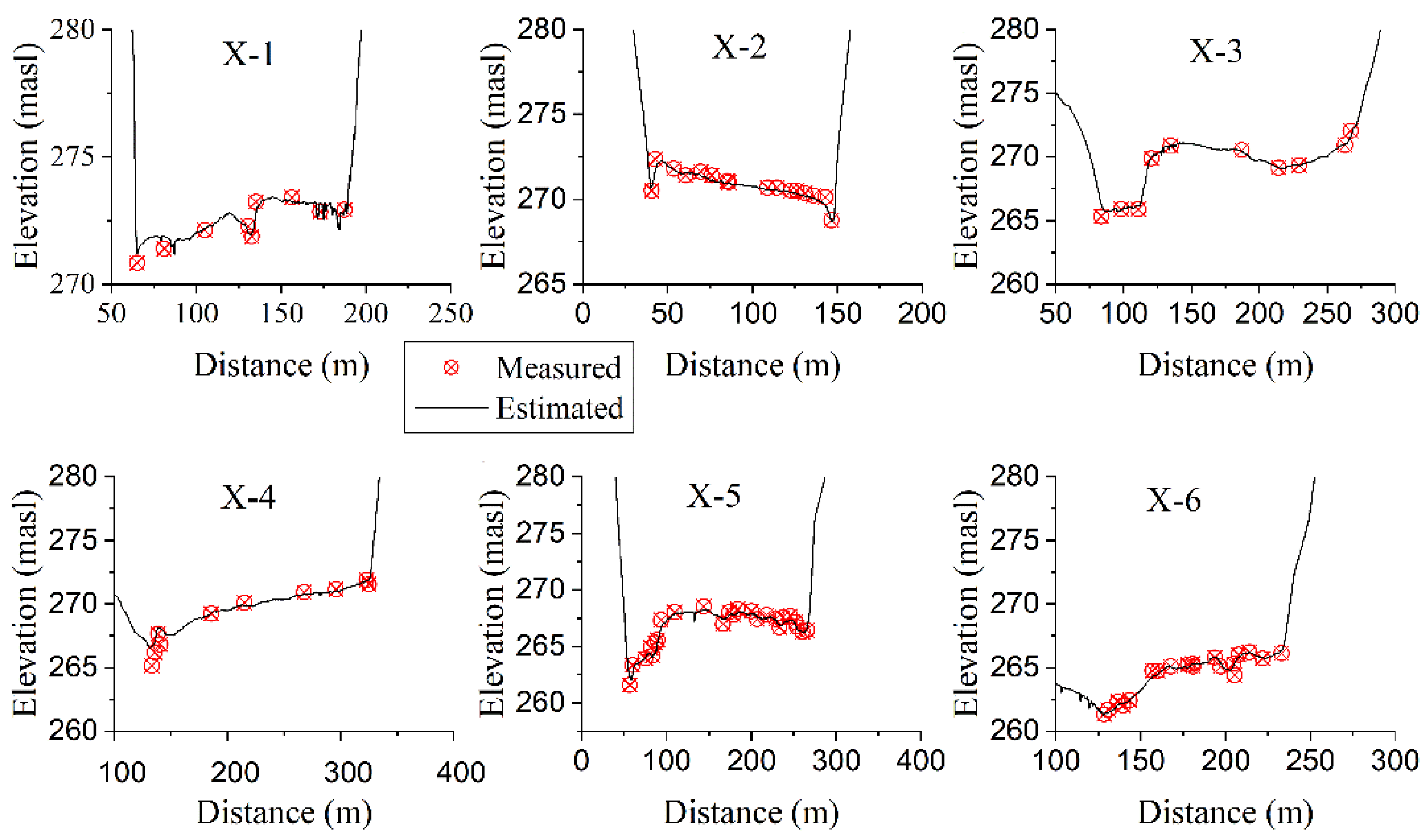
The accuracy of these 3D models was investigated by estimating errors in reproducing 3D location of points, horizontal lengths and cross sections in reference to manual measurements. Figure 3 shows errors in X, Y and Z coordinates of the selected 17 GCPs in the 3D model, designated as Ex, Ey and Ez respectively. The locations of these points were reproduced in the 3D model with maximum deviation below 4 mm in each direction and the maximum resultant error (ER) was below 5 mm. Likewise, 12 distances between random pairs of these GCPs were estimated from the 3D model and compared with respective manually measured distances (Table 2). The estimated lengths matched pretty well against respective measured distances with root mean square error (RMSE) of 1.9 mm and mean absolute error (MAE) of 1.7 mm. Moreover, 6 cross sections designated as X-1 to X-6 (Figure 1) were randomly selected over the study area and their cross-section profiles were extracted from the 3D model output for ‘After run scenario’. These estimated cross sections were compared with their respective upscaled cross-section data from manual measurements in the model (Figure 4), which showed that the estimated cross sections were close to the measured cross sections and had more detailing with abundant points.
After confirming the accuracy of DEMs produced by SfM technique to be within acceptable limits, changes in volume of river bed morphology were calculated using the DEMs generated for initial bed and after run scenarios mentioned above. At the rate of 10 kg/min for 140 min, total 1400 kg sediment was fed with the inflow discharge during the test. Using bulk density of the sediment to be 1680 m3/s, the total volume of sediment added into the system during the test was calculated to be 0.833 m3. Analysing the difference between DEMs for initial bed and river bed after simulation, it showed that 0.677 m3 (out of 0.833 m3 sediment fed into the system) sediment was deposited into whereas 0.125 m3 sediment from initially filled bed was scoured out of the system; which means total 0.281 m3 of sand was transported to downstream of the modelled river reach. To check the accuracy in estimating changes in volume, the volume of sediment trapped at the outlet tank downstream of the model was measured manually using a calibrated bucket. The measured and estimated volumes in model scale were 0.292 m3 and 0.281 m3 respectively with a discrepancy of 4% only.
After the satisfactory result from the test, SfM technique was further applied in full-fledged model study in which intermediate river bed formations at different time steps during the test were also recorded in addition to the initial and final river bed. Besides measuring the changes in bed morphology precisely, SfM technique also made it possible to record the evolution of bed morphology over time by capturing the river bed at different time steps during the test. Moreover, it provided high resolution river bed data for creating mesh of initial river bed to be used in numerical modelling. It also provided high-resolution river bed data for intermediate time steps for validating the results from the numerical model.
3.2. Case Study II: Evaluation of Sediment Flushing Efficiency
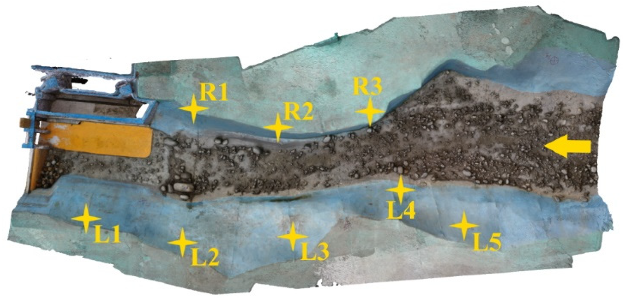
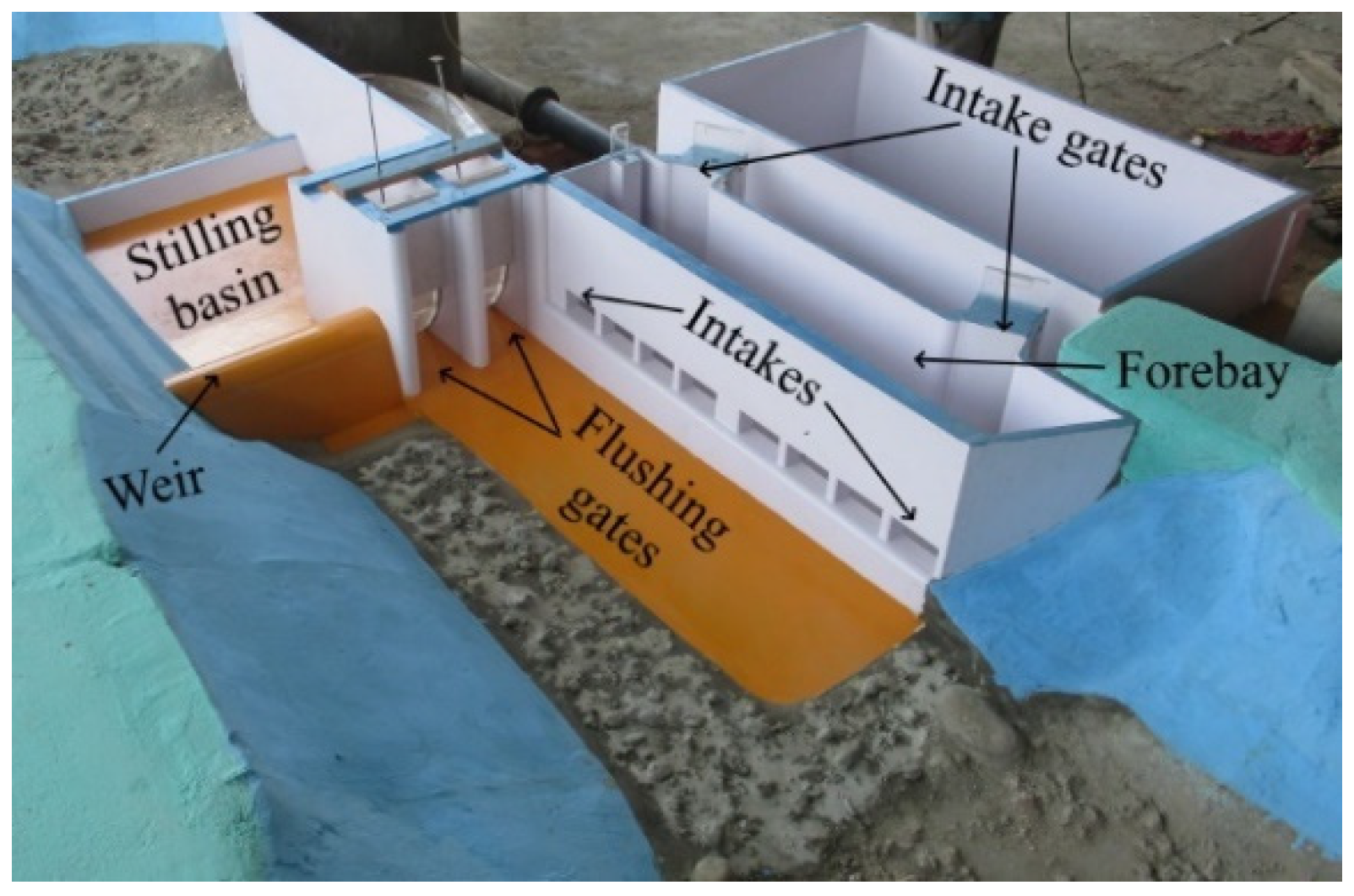
A physical hydraulic model of the headworks of a hydropower project in Khimti River of Nepal was selected to apply SfM technique in investigating flushing efficacy of headworks structures. Khimti River is a tributary of Tamakoshi River in Saptakoshi river basin. The Saptakoshi River is one of the tributaries of the Ganges River. The study area covered about 250 m reach of Khimti River upstream of the weir axis (Figure 5). The model was built as an undistorted fixed bed model on a scale of 1:40 using the Froude’s Model Law. The headworks design consisted of a free flow type gravity weir, two bed load sluices, a side intake with eight orifices and a forebay from where water is diverted towards settling basins through two gated inlet orifices. A general arrangement of the headwork is as shown in Figure 6. Since Khimti River is a typical Himalayan river with steep gradient, the hydropower plant was designed as run-off-river type. In such headworks arrangement, the pool created upstream of the diversion weir is normally insignificant and gets filled with the incoming sediment in very short time-span of operation. So, the designed headworks arrangement should be able to flush the sediment deposits around the intake area in order to avoid entry of bed sediments into the intakes. Regarding this, one of the main objectives of the model study was to ensure the capability of flushing gates to clean the deposited sediments from area around the intake upstream of the diversion weir. Since the partial opening of flushing gates in normal operation condition could not stop sedimentation in front of intakes, free flushing with annual flood discharge was tested in the model.
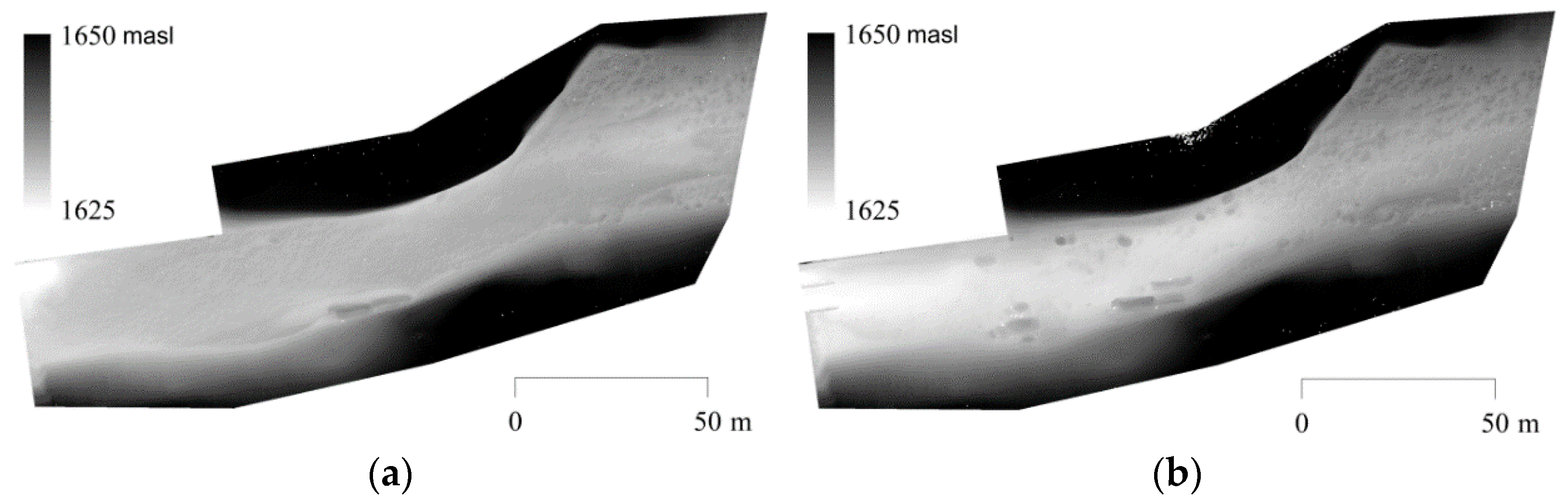
In order to speed up the sedimentation process, the river upstream of the weir was initially filled with bed sediment up to the sill level of intake orifices. The sand used for representing the bed load had median particle diameter (d50) of 1.5 mm, d10 = 0.5 mm and d90 = 10 mm. The sediment fed with the inflow discharge during the test also had the same composition. The model was run under normal operating conditions for 12 min (1.3 h in prototype) simulating a river discharge of 14.4 L/s (equivalent to annual flood with the magnitude of 146 m3/s in prototype) with sediment feeding at the rate of 0.580 kg/min which corresponds to sediment concentration of 671 ppm in the flow. Then both flushing gates were opened to allow free gravity flushing of the bed sediment with the annual flood discharge for 38 min (4 h in prototype). Initial bed before flushing and final bed after flushing were photographed and a dense point cloud for each scenario was produced in prototype scale using SfM technique in reference to 8 GCPs defined over the study area. The quality and size of dense point clouds produced with their respective processing times are presented in Table 3. The DEMs generated from the dense point clouds of the two scenarios are shown in Figure 7.
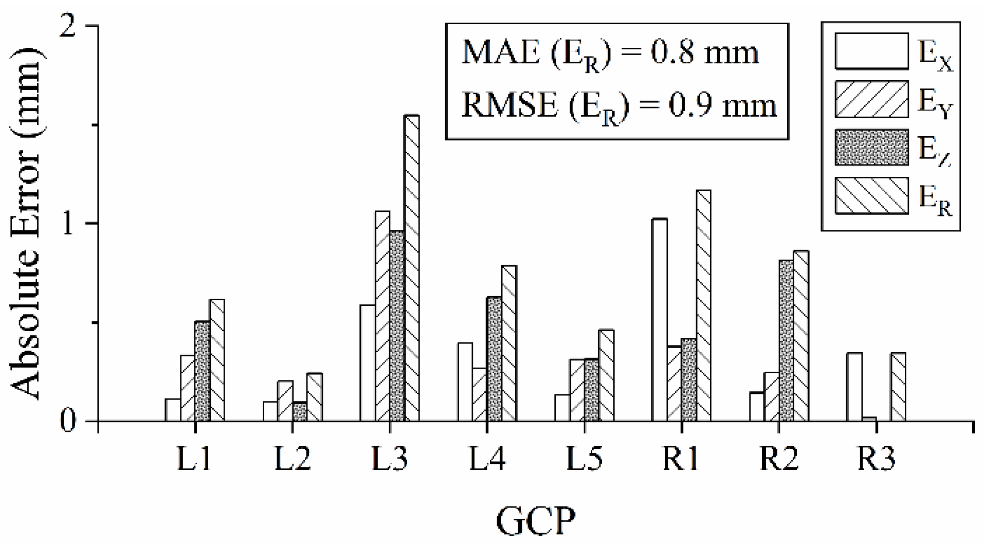
Errors in reproducing both the locations of GCPs and linear distances were calculated to be below 2 mm in the model as shown in Figure 8 and Table 4 respectively. Finally, flushing scenario was quantified by analysing the dense point clouds in CloudCompare software. Evaluating volume changes among dense point clouds for given scenarios, about 88% of sum of deposited sediment volume and volume of sediment fed was found to be flushed successfully keeping the area around the intake clean from sediment deposits. The flushed volume of sediment was estimated as a volume difference between dense cloud for initial bed before flushing and that for final bed after flushing in addition to the volume of sediment fed during the experiment. The estimated flushed volume of sediment in model scale was 0.1602 m3 against the measured volume of 0.162 m3 with only 1% of discrepancy.
In this way, the SfM technique helped to precisely quantify the bed control near intake structure in physical model studies. The SfM technique was also useful in recording spatial distribution of the sediment deposits remained upstream of the headworks after flushing, which was very useful information for the designer to identify the passive zones not cleaned by the flushing operation and to further modify, if required, the components of headworks structure to improve its overall performance. However, in this test the flushing operation was satisfactorily successful as 88% of the sediment were flushed downstream and the area around the intake was clean of sediment deposit.
3.3. Case Study III: Measurement of Flushing Cone Volume
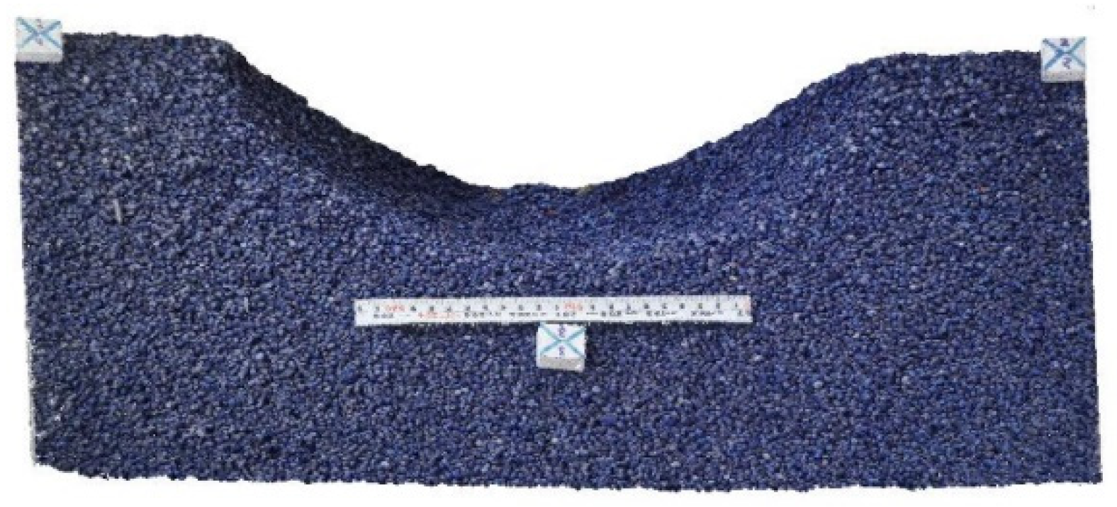
Finally, the SfM technique was applied on small scale flume experiments to investigate scour holes, commonly called as flushing cones, created by pressurized flushing of sediment deposit through a bottom outlet under steady flow conditions. The experimental setup consisted of a 0.6 m wide horizontal flume with a 50 mm wide rectangular orifice, the opening height of which was variable, at the centre of the flume. The sill of the orifice was 60 mm above the flume bed. A 120 mm thick layer of plastic grains representing sediment in the model were filled before the tests. Then a desired discharge was supplied into the flume without disturbing the filled sediment layer. When the water surface reached desired level, the bottom outlet was opened for desired opening height, which was meant to maintain the selected water level for the selected discharge, and pressurized flushing of the deposits were allowed to form a flushing cone. Once the flushing cone upstream of the outlet reached an equilibrium, the gate was closed and the flume was drained slowly without disturbing the cone. Then the flushing cone was measured manually with a millimeter precise point gauge as well as using SfM technique. Total 7 tests were carried out for different combination of discharge, water level and opening height of the outlet as listed in Table 5.
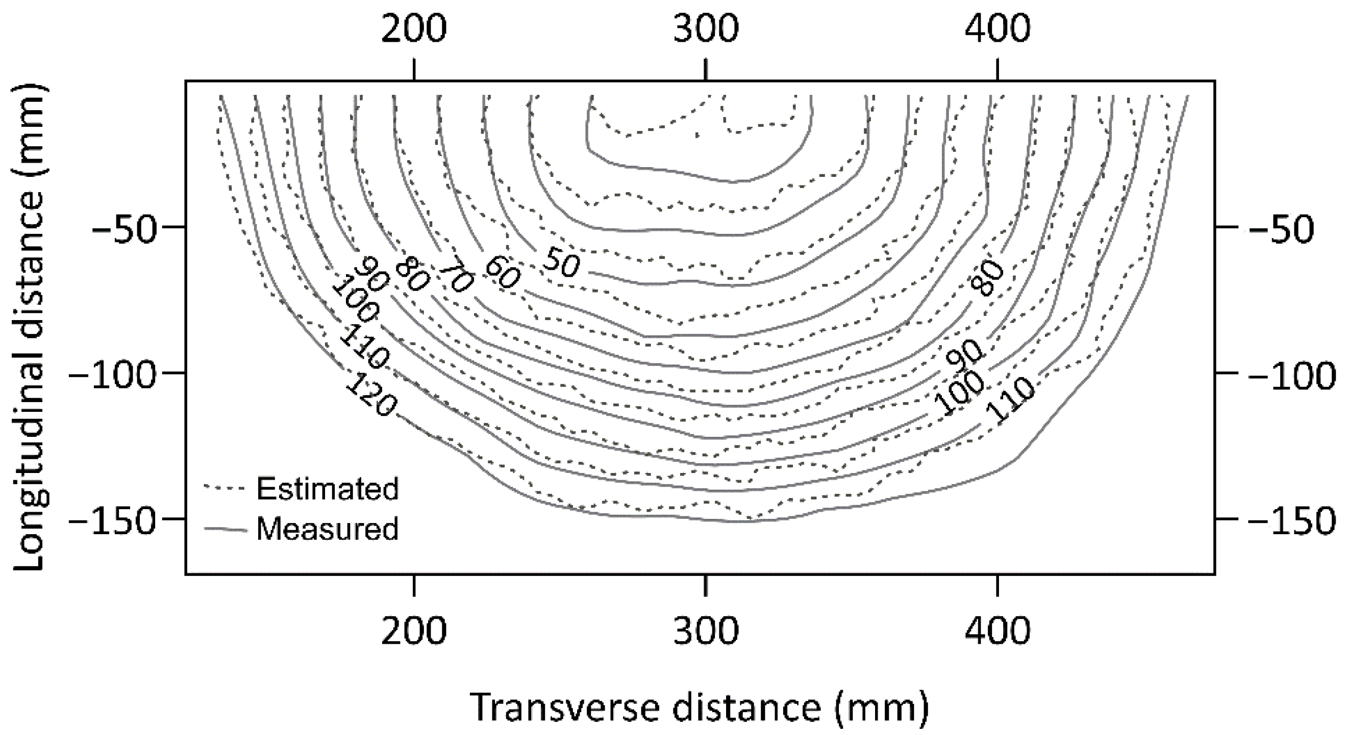
Since it was a small-scale flume test, high quality dense clouds were produced expecting better accuracy. For example, the dense point cloud for Test no. 3 is shown in Figure 9. The contour plot of flushing cone for Test no. 3 produced by SfM superimposed on that produced by manual measurements is presented in Figure 10. It shows that the flushing cone reproduced with SfM technique is comparable against the one produced by manual measurement.
The size of dense point cloud for each test and their respective processing time is shown in Table 6. The volumes of flushing cones measured manually were compared with volumes of respective cones estimated by SfM technique as shown in Table 5. The absolute discrepancy between measured and estimated volumes for all the tests were below 5% of the measured volume.
After achieving satisfactory precision from the SfM technique for such experiments, it was further applied in similar tests to produce high resolution point clouds of flushing cones which was utilized for precisely estimating dimensions and volume of flushing cones. A number of tests were carried out with varying water level, discharge, opening height of outlet, thickness of sediment deposit and density of sediment materials. The results from the experiments were used to develop empirical relations to predict the length and volume of flushing cone for relevant input parameters.
4. Discussion of Results
The overall accuracy of SfM technique was estimated to be below 5 mm for reproducing location of points and below 3 mm for estimating distance measurements in the model. Between two models in case study I and case study II, accuracy of SfM reproduced models was found to be coarser for bigger model. It can be justified with expected precision of derived elevations as defined by Lane [3]:
With de = 4 µm and c = 16 mm, the expected vertical precision for case study I and II were 0.45 mm and 0.3 mm for camera flying height of 1.79 m and 1.25 m respectively. According to Lane [3], the best possible spatial resolution is about 5 times coarser than p. From Equation (1), it can be concluded that the precision will be reduced for bigger model since camera flying height need to be increased to cover bigger area considering same camera with similar settings is used. Morgan et al. [37] also concluded that the decrease in model point count with respect to increase in distance between camera and subject follows a power law having the exponent value of approximately 2.15. The other way around to achieve output model with better accuracy is to take more pictures with lower camera flying height but it will increase the time required for image acquisition and processing.
The precision in estimating volume changes was found to be better (below 5% of measured values), most probably due to compensation of errors while subtracting two 3D models (dense point clouds or DEMs). The applicability of SfM method hence depends on acceptable error or discrepancy, which in turn is governed by scale factor for the model, objective of the model study and measurement techniques available as alternative. Analysing the results of this study, it can be concluded that SfM is a quick, economic and comparatively accurate alternative for manual measurements in the model study. The acceptability of the precision of SfM technique is entirely subjective. The same precision could be acceptable for large scale models while on the other hand it might be unacceptable for small-scale models. Besides scale factor, acceptable precision is also limited by purpose of the model study. For model studies with objectives to assess bed evolution pattern (case study I) and to estimate sediment budget (case study II and III), the achieved precision in each case studies seemed to be satisfactory. Since manual measurement with staff gauges of 1 mm precision was the only low-cost alternative available in our laboratory to SfM technique, RMSE error of 1.9 mm in output dense cloud (in model scale) is satisfactory provided with the fact that SfM technique was quicker and reproduced better detailing of important features.
The major advantage of SfM technique over manual measurement is the detailing captured as colour-coded dense point cloud. In general practice with manual measurements, only a few cross sections are selected over the study area for conducting measurements and the measured data are interpolated in-between. In such case, there is always possibility of loss or even mis-interpretation of detailing in between the measured cross sections. For example, in case study I, the front of sediment deposition was continuously moving downstream. If the deposition front was in between two measurement cross sections for a certain time step, then interpolation of manually measured two cross-section profiles upstream and downstream of that deposition front will not represent the actual pattern. Therefore, for mobile bed model studies with an objective to study patterns of bed evolution, SfM technique can ensure higher detailing of the river bed reproduced in 3D model output. Additionally, SfM technique can be highly beneficial to capture the time-evolution of the river bed morphology by taking set of photographs at certain intervals of model run time. It can save a significant amount of time compared to measurements carried out with manual instrumentation. Though processing time for SfM technique could extend up to couple of hours, e.g., more than 4 h for producing 3D dense point cloud of initial filled bed in Case study I as shown in Table 1, actual man-hour used will be much lower since the image processing up to production of 3D models can be fully automatized. Moreover, the total processing time can also be reduced considerably by targeting low or medium quality of dense point cloud yet ensuring the quality of result will not be compromised.
The results from all three case studies (see Table 1, Table 3 and Table 6) showed that the image processing time in SfM is not proportional to the number of images to be processed. While doing trials to produce 3D models of different quality (low, medium and high), it was observed that the processing time for same set of images increased as the desired output (dense point cloud) quality was set from low to medium and then to high.
5. Conclusions
SfM photogrammetry technique was successfully applied in three different model studies to estimate changes in mobile river bed. Free handheld photography was used for acquiring images which reduced the logistical cost for camera support setup and also reduced the image acquisition time. The 3D models in form of dense point clouds were produced with satisfactory precision against manual measurement using lesser time and human resources. Hence, SfM is recommended as a low-cost and quicker alternative to manual measurements in physical hydraulic models. However, the selection of measurement technique is always a trade-off between desired precision, time spent for measurement and data analysis, and total budget (cost) incurred.
Author Contributions
Conceptualization: N.R., S.K.K.; Methodology: S.K.K., U.S.; Resources: N.R., M.B.B.; Investigation: S.K.K., U.S.; Formal analysis: S.K.K., U.S.; Software: S.K.K., U.S.; Validation: N.R.; Visualization: S.K.K., U.S.; Data curation: S.K.K., U.S.; Writing-original draft: S.K.K.; Writing-review & editing: S.K.K.; Supervision: N.R.; Project administration: N.R., M.B.B.; Funding acquisition: N.R., M.B.B. All authors have read and agreed to the published version of the manuscript.
Funding
This research was funded by The Research Council of Norway, Hydro Lab, Statkraft and the Norwegian Hydropower Center (NVKS).
Institutional Review Board Statement
Not applicable.
Informed Consent Statement
Not applicable.
Data Availability Statement
3rd Party Data.
Acknowledgments
We would like to thank all the technicians and colleagues at Hydro Lab, Nepal for the help and support during the study.
Conflicts of Interest
The authors declare no conflict of interest.
References
- Aberle, J.; Rennie, C.D.; Admiraal, D.M.; Muste, M. Experimental Hydraulics: Methods, Instrumentation, Data Processing and Management: Volume II: Instrumentation and Measurement Techniques, 1st ed.; Aberle, J., Rennie, C., Admiraal, D., Muste, M., Eds.; CRC Press: Boca Raton, FL, USA, 2017; ISBN 978-1-315-15892-1. [Google Scholar]
- Lane, S.N.; Richards, K.S.; Chandler, J.H. Developments in Photogrammetry; the Geomorphological Potential. Prog. Phys. Geogr. Earth Environ. 1993, 17, 306–328. [Google Scholar] [CrossRef]
- Lane, S.N.; Chandler, J.H.; Porfiri, K. Monitoring River Channel and Flume Surfaces with Digital Photogrammetry. J. Hydraul. Eng. 2001, 127, 871–877. [Google Scholar] [CrossRef]
- Chandler, J.H.; Shiono, K.; Rameshwaren, P.; Lane, S.N. Measuring Flume Surfaces for Hydraulics Research Using a Kodak DCS460. Photogramm. Rec. 2001, 17, 39–61. [Google Scholar] [CrossRef]
- Smith, M.W.; Carrivick, J.L.; Quincey, D.J. Structure from Motion Photogrammetry in Physical Geography. Prog. Phys. Geogr. 2016, 40, 247–275. [Google Scholar] [CrossRef] [Green Version]
- Skarlatos, D.; Kiparissi, S. Comparison of Laser Scanning, Photogrammetry and SFM-MVS Pipeline Applied in Structures and Artificial Surfaces. ISPRS Ann. Photogramm. Remote Sens. Spat. Inf. Sci. 2012, I-3, 299–304. [Google Scholar] [CrossRef] [Green Version]
- Remondino, F.; El-Hakim, S. Image-Based 3D Modelling: A Review. Photogramm. Rec. 2006, 21, 269–291. [Google Scholar] [CrossRef]
- Acuna, M.; Sosa, A. Automated Volumetric Measurements of Truckloads through Multi-View Photogrammetry and 3D Reconstruction Software. Croat. J. For. Eng. J. Theory Appl. For. Eng. 2019, 40, 151–162. [Google Scholar]
- Westoby, M.J.; Brasington, J.; Glasser, N.F.; Hambrey, M.J.; Reynolds, J.M. ‘Structure-from-Motion’ Photogrammetry: A Low-Cost, Effective Tool for Geoscience Applications. Geomorphology 2012, 179, 300–314. [Google Scholar] [CrossRef] [Green Version]
- Favalli, M.; Fornaciai, A.; Isola, I.; Tarquini, S.; Nannipieri, L. Multiview 3D Reconstruction in Geosciences. Comput. Geosci. 2012, 44, 168–176. [Google Scholar] [CrossRef] [Green Version]
- Wu, C. Towards Linear-Time Incremental Structure from Motion. In Proceedings of the 2013 International Conference on 3D Vision—3DV 2013, Seattle, WA, USA, 29 June–1 July 2013; pp. 127–134. [Google Scholar]
- Eltner, A.; Sofia, G. Structure from motion photogrammetric technique. In Developments in Earth Surface Processes; Elsevier: Amsterdam, The Netherlands, 2020; Volume 23, pp. 1–24. ISBN 978-0-444-64177-9. [Google Scholar] [CrossRef]
- Smith, M.W.; Vericat, D. From Experimental Plots to Experimental Landscapes: Topography, Erosion and Deposition in Sub-Humid Badlands from Structure-from-Motion Photogrammetry. Earth Surf. Process. Landf. 2015, 40, 1656–1671. [Google Scholar] [CrossRef] [Green Version]
- Snavely, K.N. Scene Reconstruction and Visualization from Internet Photo Collections. Ph.D. Thesis, University of Washington, Seattle, WA, USA, 2009. [Google Scholar]
- James, M.R.; Robson, S. Straightforward Reconstruction of 3D Surfaces and Topography with a Camera: Accuracy and Geoscience Application. J. Geophys. Res. Earth Surf. 2012, 117, F03017. [Google Scholar] [CrossRef] [Green Version]
- Goesele, M.; Snavely, N.; Curless, B.; Hoppe, H.; Seitz, S.M. Multi-View Stereo for Community Photo Collections. In Proceedings of the 2007 IEEE 11th International Conference on Computer Vision, Rio de Janeiro, Brazil, 14–21 October 2007; pp. 1–8. [Google Scholar]
- James, M.R.; Chandler, J.H.; Eltner, A.; Fraser, C.; Miller, P.E.; Mills, J.P.; Noble, T.; Robson, S.; Lane, S.N. Guidelines on the Use of Structure-from-Motion Photogrammetry in Geomorphic Research. Earth Surf. Process. Landf. 2019, 44, 2081–2084. [Google Scholar] [CrossRef]
- Szabó, G.; Bertalan, L.; Barkóczi, N.; Kovács, Z.; Burai, P.; Lénárt, C. Zooming on Aerial Survey. In Small Flying Drones: Applications for Geographic Observation; Casagrande, G., Sik, A., Szabó, G., Eds.; Springer International Publishing: Cham, Switzerland, 2018; pp. 91–126. ISBN 978-3-319-66577-1. [Google Scholar]
- Micheletti, N.; Chandler, J.; Lane, S.N. Structure from Motion (SFM) Photogrammetry. In Geomorphological Techniques (Online Edition); Cook, S.J., Clarke, L.E., Nield, J.M., Eds.; British Society for Geomorphology: London, UK, 2015. [Google Scholar]
- Lane, S.N. The Measurement of River Channel Morphology Using Digital Photogrammetry. Photogramm. Rec. 2000, 16, 937–961. [Google Scholar] [CrossRef]
- Hartley, R.; Zisserman, A. Multiple View Geometry in Computer Vision, 2nd ed.; Cambridge University Press: Cambridge, UK, 2004; ISBN 978-0-521-54051-3. [Google Scholar]
- Leduc, P.; Peirce, S.; Ashmore, P. Short Communication: Challenges and Applications of Structure-from-Motion Photogrammetry in a Physical Model of a Braided River. Earth Surf. Dyn. 2019, 7, 97–106. [Google Scholar] [CrossRef] [Green Version]
- Carrivick, J.L.; Smith, M.W. Fluvial and Aquatic Applications of Structure from Motion Photogrammetry and Unmanned Aerial Vehicle/Drone Technology. Wiley Interdiscip. Rev. Water 2019, 6, e1328. [Google Scholar] [CrossRef] [Green Version]
- Alfredsen, K.; Haas, C.; Tuhtan, J.A.; Zinke, P. Brief Communication: Mapping River Ice Using Drones and Structure from Motion. Cryosphere 2018, 12, 627–633. [Google Scholar] [CrossRef] [Green Version]
- Atkinson, K. Close Range Photogrammetry and Machine Vision; Whittles Publ.: Dunbeath, UK, 1996. [Google Scholar]
- Bemis, S.P.; Micklethwaite, S.; Turner, D.; James, M.R.; Akciz, S.; Thiele, S.T.; Bangash, H.A. Ground-Based and UAV-Based Photogrammetry: A Multi-Scale, High-Resolution Mapping Tool for Structural Geology and Paleoseismology. J. Struct. Geol. 2014, 69, 163–178. [Google Scholar] [CrossRef]
- Mancini, F.; Dubbini, M.; Gattelli, M.; Stecchi, F.; Fabbri, S.; Gabbianelli, G. Using Unmanned Aerial Vehicles (UAV) for High-Resolution Reconstruction of Topography: The Structure from Motion Approach on Coastal Environments. Remote Sens. 2013, 5, 6880–6898. [Google Scholar] [CrossRef] [Green Version]
- Gindraux, S.; Boesch, R.; Farinotti, D. Accuracy Assessment of Digital Surface Models from Unmanned Aerial Vehicles’ Imagery on Glaciers. Remote Sens. 2017, 9, 186. [Google Scholar] [CrossRef] [Green Version]
- Micheletti, N.; Chandler, J.H.; Lane, S.N. Investigating the Geomorphological Potential of Freely Available and Accessible Structure-from-Motion Photogrammetry Using a Smartphone. Earth Surf. Process. Landf. 2015, 40, 473–486. [Google Scholar] [CrossRef] [Green Version]
- Abdelaziz, M.; Elsayed, M. Underwater Photogrammetry Digital Surface Model (DSM) of the Submerged Site of the Ancient Lighthouse Near Qaitbay Fort In Alexandria, Egypt. Int. Arch. Photogramm. Remote Sens. Spat. Inf. Sci. 2019, XLII-2/W10, 1–8. [Google Scholar] [CrossRef] [Green Version]
- Jones, C.A.; Church, E. Photogrammetry Is for Everyone: Structure-from-Motion Software User Experiences in Archaeology. J. Archaeol. Sci. Rep. 2020, 30, 102261. [Google Scholar] [CrossRef]
- Sapirstein, P.; Murray, S. Establishing Best Practices for Photogrammetric Recording During Archaeological Fieldwork. J. Field Archaeol. 2017, 42, 337–350. [Google Scholar] [CrossRef]
- Lerma, J.L.; Muir, C. Evaluating the 3D Documentation of an Early Christian Upright Stone with Carvings from Scotland with Multiples Images. J. Archaeol. Sci. 2014, 46, 311–318. [Google Scholar] [CrossRef]
- Andreff, N.; Horaud, R.; Espiau, B. Robot Hand-Eye Calibration Using Structure-from-Motion. Int. J. Robot. Res. 2001, 20, 228–248. [Google Scholar] [CrossRef] [Green Version]
- Schmidt, J.; Vogt, F.; Niemann, H. Calibration–Free Hand–Eye Calibration: A Structure–from–Motion Approach. In Pattern Recognition; Kropatsch, W.G., Sablatnig, R., Hanbury, A., Eds.; Springer: Berlin/Heidelberg, Germany, 2005; Volume 3663, pp. 67–74. ISBN 978-3-540-28703-2. [Google Scholar]
- Heller, J.; Havlena, M.; Sugimoto, A.; Pajdla, T. Structure-from-Motion Based Hand-Eye Calibration Using L∞ Minimization. In Proceedings of the CVPR 2011, Colorado Springs, CO, USA, 20–25 June 2011; pp. 3497–3503. [Google Scholar]
- Morgan, J.A.; Brogan, D.J.; Nelson, P.A. Application of Structure-from-Motion Photogrammetry in Laboratory Flumes. Geomorphology 2017, 276, 125–143. [Google Scholar] [CrossRef] [Green Version]
- Balaguer-Puig, M.; Marqués-Mateu, Á.; Lerma, J.L.; Ibáñez-Asensio, S. Estimation of Small-Scale Soil Erosion in Laboratory Experiments with Structure from Motion Photogrammetry. Geomorphology 2017, 295, 285–296. [Google Scholar] [CrossRef]
- Hwang, K.S.; Hwung, H.H.; Shi, B.T. Applying Photogrammetry in Laboratory Bathymetry Measurement. In Proceedings of the 13th Asian Symposium on Visualisation, Novosibirsk, Russia, 22–26 June 2015. [Google Scholar]
- Di Bacco, M.; Scorzini, A.R. Experimental Analysis on Sediment Transport Phenomena in Channels Equipped with Inclined Side Weirs. In Proceedings of the Proceedings of the 8th IAHR International Symposium on Hydraulic Structures ISHS2020, The University of Queensland, Santiago, Chile, 1 January 2020. [Google Scholar]
- Ferreira, E.; Chandler, J.; Wackrow, R.; Shiono, K. Automated Extraction of Free Surface Topography Using SfM-MVS Photogrammetry. Flow Meas. Instrum. 2017, 54, 243–249. [Google Scholar] [CrossRef] [Green Version]
- van Scheltinga, R.C.T.; Coco, G.; Kleinhans, M.G.; Friedrich, H. Observations of Dune Interactions from DEMs Using Through-Water Structure from Motion. Geomorphology 2020, 359, 107126. [Google Scholar] [CrossRef]
- Kasprak, A.; Wheaton, J.M.; Ashmore, P.E.; Hensleigh, J.W.; Peirce, S. The Relationship between Particle Travel Distance and Channel Morphology: Results from Physical Models of Braided Rivers. J. Geophys. Res. Earth Surf. 2015, 120, 55–74. [Google Scholar] [CrossRef]
- Yang, M.-D.; Chao, C.-F.; Huang, K.-S.; Lu, L.-Y.; Chen, Y.-P. Image-Based 3D Scene Reconstruction and Exploration in Augmented Reality. Autom. Constr. 2013, 33, 48–60. [Google Scholar] [CrossRef]
- Chandler, J. Effective application of automated digital photogrammetry for geomorphological research. Earth Surf. Process. Landf. 1999, 24, 51–63. [Google Scholar] [CrossRef]
- Oniga, V.-E.; Breaban, A.-I.; Statescu, F. Determining the Optimum Number of Ground Control Points for Obtaining High Precision Results Based on UAS Images. Proceedings 2018, 2, 352. [Google Scholar] [CrossRef] [Green Version]
- Tonkin, T.; Midgley, N. Ground-Control Networks for Image Based Surface Reconstruction: An Investigation of Optimum Survey Designs Using UAV Derived Imagery and Structure-from-Motion Photogrammetry. Remote Sens. 2016, 8, 786. [Google Scholar] [CrossRef] [Green Version]
- Turner, D.; Lucieer, A.; Wallace, L. Direct Georeferencing of Ultrahigh-Resolution UAV Imagery. IEEE Trans. Geosci. Remote Sens. 2014, 52, 2738–2745. [Google Scholar] [CrossRef]
- Karmacharya, S.K.; Bishwakarma, M.; Shrestha, U.; Rüther, N. Application of ‘Structure from Motion’ (SfM) Technique in Physical Hydraulic Modelling. J. Phys. Conf. Ser. 2019, 1266, 012008. [Google Scholar] [CrossRef]
- Agisoft. Agisoft PhotoScan User Manual—Standard Edition, Version 1.4; Agisoft LLC: St. Petersburg, Russia, 2018; p. 66. [Google Scholar]
- Kamphuis, J.W. Practical Scaling of Coastal Models. Coast. Eng. Proc. 1974, 121. [Google Scholar] [CrossRef] [Green Version]
- Kobus, H. Hydraulic Modelling; German Association for Water Research and Land Development: Berlin, Germany, 1980. [Google Scholar]
Figure 1.
Trishuli River model with locations of 17 GCPs (R1-R10 in the right bank and L1-L7 in the left bank) and 6 measurement cross-sections (X-1 to X-6). The figure shows the fixed bed river model which is then filled with mobile sediment bed.
Figure 1.
Trishuli River model with locations of 17 GCPs (R1-R10 in the right bank and L1-L7 in the left bank) and 6 measurement cross-sections (X-1 to X-6). The figure shows the fixed bed river model which is then filled with mobile sediment bed.

Figure 2.
DEMs produced by SfM technique for Case Study I: (a) initial mobile bed; (b) final bed after test run.
Figure 2.
DEMs produced by SfM technique for Case Study I: (a) initial mobile bed; (b) final bed after test run.

Figure 3.
Estimated errors in reproduction of points in a 3D model using SfM, Case Study I. The errors are calculated in model scale.
Figure 3.
Estimated errors in reproduction of points in a 3D model using SfM, Case Study I. The errors are calculated in model scale.

Figure 4.
Plots of cross-sections estimated by SfM and manually measured cross-sections upscaled to prototype scale.
Figure 4.
Plots of cross-sections estimated by SfM and manually measured cross-sections upscaled to prototype scale.

Figure 5.
Khimti River model with location of 8 GCPs (R1-R3 in the right bank and L1-L5 in the left bank). The figure shows the fixed bed river model which is then filled with mobile sediment bed.
Figure 5.
Khimti River model with location of 8 GCPs (R1-R3 in the right bank and L1-L5 in the left bank). The figure shows the fixed bed river model which is then filled with mobile sediment bed.

Figure 6.
Headworks structure arrangement under study, Case study II.

Figure 7.
DEMs produced by SfM technique for Case Study II: (a) initial mobile bed; (b) final bed after flushing test.
Figure 7.
DEMs produced by SfM technique for Case Study II: (a) initial mobile bed; (b) final bed after flushing test.

Figure 8.
Estimated errors in reproduction of points in a 3D model using SfM, Case Study II. The errors were estimated in model scale.
Figure 8.
Estimated errors in reproduction of points in a 3D model using SfM, Case Study II. The errors were estimated in model scale.

Figure 9.
Dense point cloud of flushing cone for Test no. 3, Case study III.

Figure 10.
Contour plots for Test no. 3 by SfM estimation and Manual measurement in model scale, Case study III.
Figure 10.
Contour plots for Test no. 3 by SfM estimation and Manual measurement in model scale, Case study III.


Table 1.
Processing time and output quality for Case study I.
| Stage | No. of Images | Time for Feature Matching and Alignment | Time to Create Dense Cloud | Time to Create DEM | Quality of Dense Cloud | No. of Vertices in Dense Point Cloud |
|---|---|---|---|---|---|---|
| Initial Bed | 244 | 31 min | 4 h | 18 min | medium | 30.36 million |
| After Run | 116 | 46 min | 49 min | 15 min | medium | 23.45 million |
Table 2.
Estimated errors in reproduction of selected distances in the 3D model by SfM, Case Study I.
Table 2.
Estimated errors in reproduction of selected distances in the 3D model by SfM, Case Study I.
| Distance between GCPs | Distance by Manual Measurement, mm | Distance from 3D Model by SfM, mm | Absolute Discrepancy, mm |
|---|---|---|---|
| LA-R1 | 1879.15 | 1877.00 | 2.2 |
| L1-R2 | 1861.60 | 1862.00 | 0.4 |
| L2-RA | 2466.94 | 2465.00 | 1.9 |
| L2-R3 | 2132.04 | 2135.00 | 3.0 |
| L5-R5 | 3793.81 | 3796.00 | 2.2 |
| L5-R9 | 3909.81 | 3912.00 | 2.2 |
| L7-R10 | 2594.69 | 2597.00 | 2.3 |
| L6-R9 | 2543.95 | 2544.00 | 0.0 |
| L5-R7 | 2893.94 | 2895.00 | 1.1 |
| L6-R8 | 2568.95 | 2571.00 | 2.0 |
| L4-R6 | 3245.66 | 3245.00 | 0.7 |
| L5-R4 | 4422.73 | 4425.00 | 2.3 |
Table 3.
Processing time and output quality for Case study II.
| Stage | No. of Images | Time for Feature Matching and Alignment | Time to Create Dense Cloud | Time to Create DEM | Quality of Dense Cloud | No. of Vertices in Dense Point Cloud |
|---|---|---|---|---|---|---|
| Initial Bed | 61 | 6 min | 57min | 9 min | medium | 13.21 Million |
| After Run | 74 | 14 min | 1 h 7 min | 11 min | medium | 16.13 Million |
Table 4.
Estimated errors in reproduction of selected distances in the 3D model by SfM, Case Study II.
Table 4.
Estimated errors in reproduction of selected distances in the 3D model by SfM, Case Study II.
| Distance between GCPs | Distance by Manual Measurement, mm | Distance from 3D Model by SfM, mm | Absolute Discrepancy, mm |
|---|---|---|---|
| L1-R1 | 1550.35 | 1550.0 | 0.35 |
| L2-R1 | 1326.82 | 1328.0 | 1.18 |
| L4-R3 | 1121.20 | 1121.0 | 0.20 |
| L5-R5 | 1858.53 | 1857.0 | 1.53 |
| L2-R5 | 4101.46 | 4100.0 | 1.46 |
| R1-R2 | 851.83 | 852.0 | 0.17 |
| R2-R3 | 911.97 | 913.0 | 1.03 |
Table 5.
Boundary conditions and measured volume of flushing cone for tests conducted in Case Study III.
Table 5.
Boundary conditions and measured volume of flushing cone for tests conducted in Case Study III.
| Test No. | Discharge, L/s | Water Level, mm | Outlet’s Opening Height, mm | Volume of Flushing Cone, ×106 mm3 | Absolute Discrepancy % | |
|---|---|---|---|---|---|---|
| Manual Measurement | Measured from 3D Model by SfM | |||||
| 1 | 2.5 | 244 | 40 | 1.31 | 1.27 | 3.05 |
| 2 | 3.2 | 352 | 40 | 1.54 | 1.54 | 0.00 |
| 3 | 3.9 | 455 | 40 | 1.72 | 1.78 | 3.49 |
| 4 | 4.3 | 570 | 40 | 1.80 | 1.77 | 1.67 |
| 5 | 3.2 | 264 | 50 | 1.48 | 1.41 | 4.73 |
| 6 | 3.8 | 327 | 50 | 1.63 | 1.67 | 2.45 |
| 7 | 5.0 | 502 | 50 | 1.98 | 1.99 | 0.51 |
Table 6.
Processing time and output quality for Case study III.
| Test No. | No. of Images | Total Processing Time to Create Dense Cloud (hh:mm:ss) | Quality of Dense Cloud | Points in Dense Cloud (in Millions) |
|---|---|---|---|---|
| 1 | 18 | 00:48:27 | high | 13.7 |
| 2 | 24 | 01:08:21 | high | 15.5 |
| 3 | 18 | 00:31:38 | high | 12.6 |
| 4 | 28 | 01:11:44 | high | 15.3 |
| 5 | 22 | 01:03:15 | high | 14.3 |
| 6 | 30 | 02:54:23 | high | 15.8 |
| 7 | 27 | 02:08:32 | high | 18.6 |
Publisher’s Note: MDPI stays neutral with regard to jurisdictional claims in published maps and institutional affiliations. |
© 2021 by the authors. Licensee MDPI, Basel, Switzerland. This article is an open access article distributed under the terms and conditions of the Creative Commons Attribution (CC BY) license (https://creativecommons.org/licenses/by/4.0/).
Share and Cite
MDPI and ACS Style
Karmacharya, S.K.; Ruther, N.; Shrestha, U.; Bishwakarma, M.B. Evaluating the Structure from Motion Technique for Measurement of Bed Morphology in Physical Model Studies. Water 2021, 13, 998. https://doi.org/10.3390/w13070998
AMA Style
Karmacharya SK, Ruther N, Shrestha U, Bishwakarma MB. Evaluating the Structure from Motion Technique for Measurement of Bed Morphology in Physical Model Studies. Water. 2021; 13(7):998. https://doi.org/10.3390/w13070998
Chicago/Turabian StyleKarmacharya, Sanat Kumar, Nils Ruther, Ujjwal Shrestha, and Meg Bahadur Bishwakarma. 2021. "Evaluating the Structure from Motion Technique for Measurement of Bed Morphology in Physical Model Studies" Water 13, no. 7: 998. https://doi.org/10.3390/w13070998
Note that from the first issue of 2016, this journal uses article numbers instead of page numbers. See further details here.