Introducing Non-Stationarity Into the Development of Intensity-Duration-Frequency Curves under a Changing Climate

Abstract

Intensity-duration-frequency (IDF) relationships are traditional tools in water infrastructure planning and design. IDFs are developed under a stationarity assumption which may not be realistic, neither in the present nor in the future, under a changing climatic condition. This paper introduces a framework for generating non-stationary IDFs under climate change, assuming that probability of occurrence of quantiles changes over time. Using Extreme Value Theory, eight trend combinations in Generalized Extreme Value (GEV) parameters using time as covariate are compared with a stationary GEV, to identify the best alternative. Additionally, a modified Equidistance Quantile Matching (EQM_NS) method is implemented to develop IDFs for future conditions, introducing non-stationarity where justified, based on the Global Climate Models (GCM). The methodology is applied for Moncton and Shearwater gauges in Northeast Canada. From the results, it is observed that EQM_NS is able to capture the trends in the present and to translate them to estimated future rainfall intensities. Comparison of present and future IDFs strongly suggest that return period can be reduced by more than 50 years in the estimates of future rainfall intensities (e.g., historical 100-yr return period extreme rainfall may have frequency smaller than 50-yr under future conditions), raising attention to emerging risks to water infrastructure systems.

1. Introduction

Extreme precipitation is expected to increase in intensity and magnitude due to the effects of global warming, also recognized as climate change [1,2]. Changes in patterns of climate have already been observed in many parts of the globe since the last century [3]. In urban areas, the rise of intense precipitation can negatively impact the urban infrastructure, economic activities, and social well-being through the drainage system overflow and resulting flooding events.

The intensity-duration-frequency (IDF) curve is one of the most traditional tools for engineering planning and design of various urban infrastructure systems, including urban drainage infrastructure and flood protection measures. The IDF curves are generated based on a stationary frequency-based analysis of historical annual maximum precipitation for a given duration, which assumes that the frequency of occurrence of extreme precipitation remains constant over time. However, under a changing climate, current IDF curves may be underestimating rainfall intensity because: (i) IDF curves are developed for earlier climatic conditions that may not be adequately representing future conditions [4]; (ii) IDF curves are developed based on an assumption of stationarity which may not be valid anymore [5,6]; and (iii) combination of (i) and (ii). For previously mentioned scenarios, a frequent overload of the water infrastructure systems is expected, resulting in an increase in probability of failure. Given the effects of climate change and non-stationarity on IDFs, it is necessary to investigate new methods for their development [7]. The development of future climate based IDF curves has been explored in the literature to some extent [8,9,10,11,12]. Most of the research is using precipitation outputs from Global Climate Models (GCMs) that simulate future climate states for different scenarios of radiative forcing, the Representative Concentration Pathways (RCPs) [2]. Climate projection data from GCMs are of great value, in spite of coarse spatial and temporal resolutions (usual grid size is 100 by 100 km) [11] which may lead to misrepresentation of extreme rainfall events and high uncertainty [7,13], especially for precipitation events with low frequency (large return period). That limitation can be addressed with the use of downscaling (dynamic or statistical) techniques.

Dynamic downscaling reduces the scale by refining climate processes and simulating local conditions, generating small spatiotemporal gridded Regional Climate Models (RCMs) (usually from 25 to 50 km and sub-daily time step). In general, for urban drainage engineering and planning, RCMs are recommended for local rainfall extreme analysis, given their representation of the convective processes that dominate short-duration rainfall extremes and the higher precision and accuracy when compared to the GCMs [14,15]. High-resolution RCMs, as examples of convection-permitting climate models (about 1 km), allow the explicit simulation of atmospheric deep convection and improve the representation of orography and land-surface interactions [16,17]. However, climate models often provide biased representations of observed time series [18] and RCMs inherit the biases and other deficiencies from the GCMs, and hence further (statistical) downscaling is often necessary for RCM projections [19]. The fundamental assumption of the statistical downscaling is to correct the biases presented in climate model products compared to the observed data [20]. There are several methods to manage bias correction but performance of all is highly dependent on the goal of the study. Specially, for updating future IDF curves studies, statistical downscaling is used as the main process since time scales as low as 10 min can be necessary [7]. Among the existing statistical downscaling methods, those which consider both spatial and temporal downscaling have received significant attention [8,9,11,14,21,22]. Those methods that include the downscaling of the whole rainfall series remain less certain since they cannot adequately represent the frequency of rainfall extremes [23]. The quantile-mapping based downscaling methods focus on downscaling extreme rainfall quantiles and reduces the error propagation [9,11,24,25]. However, the use of quantile-mapping based statistical downscaling models including an assumption that the relationship between GCM and the observed data remains the same for projected future period, and does not account for the non-stationarity inherent in the climate change context [11].

Non-stationarity of precipitation is characterized by a variation in the form of a trend or oscillation in the patterns of a rainfall time series. Based on recent theoretical developments in the Extreme Value Theory (EVT), several studies investigated development of non-stationary rainfall IDF curve [6,26,27]. In general, different trend functions can introduce one or more covariates, and their combinations, in the parameters of probability distributions, such as Generalized Extreme Value (GEV) and peaks-over-threshold (POT) Generalized Pareto Distribution (GPD). Linear trend functions are the most frequently used for the development of non-stationary IDF curves. They are applied to different parameters, such as, for example, the location parameter of the GEV distribution [26], location and shape parameters [27], or the scale parameter of the GPD distribution [28].

Quantile-mapping-based downscaling methods have been used to develop future IDF curves under climate change over Canada [29,30]. The original methodology, as proposed by [11], named Equidistance Quantile Matching method (EQM), incorporates the changes in the distribution characteristics of the GCM model between the baseline and projected periods. Even though there are advances in improving the projections of future IDFs, only a few studies include assessment or consideration of the non-stationary behavior of the precipitation data. A recent research carried by [14] assessed the effects of non-stationarity on the IDF curves by comparison with stationary IDFs, using climate change projections over the Southern Ontario, Canada. The authors used the RCM outputs and bias-correction for generating future annual maxima precipitation (AMP) time series. Their statistics are further modeled by taking into account the non-stationarity and introduction of the linear trend in the location parameter of GEV distribution. This implies that non-stationarity is considered after the statistical downscaling, ignoring its possible effects even in the reference period (i.e., present).

Note that the several approaches using non-stationarity in IDF relationships have been reported in the literature [6,26,27]. In addition, studies of non-stationarity in future IDF relationships under climate change are already ongoing [14]. However, to the authors’ best knowledge, no research was reported which (i) considered non-stationary modelling conditions to the reference period before the downscaling procedure to generate future AMP series in the projected period, and then (ii) developed non-stationary future IDF curves under climate change. Using the EQM algorithm, this study aims to assess and develop non-stationary GEV models, and non-stationary IDF relationships under climate change. Unlike the straightforward application of non-stationarity in modeling GEV parameters, this new framework to update IDF curves (called EQM_NS) is based on statistical analysis which identifies if the non-stationary GEV model is the best GEV model fitted to the data. Time is adopted as a covariate in the location and scale parameters of the GEV distribution. Different time-variant and trend functions lead to eight combinations of non-stationary models which are considered in this study together with one stationary GEV model. The new framework is applied to Moncton City gauging station data in the Province of New Brunswick, Canada, in order to analyze its performance in developing future IDF curves.

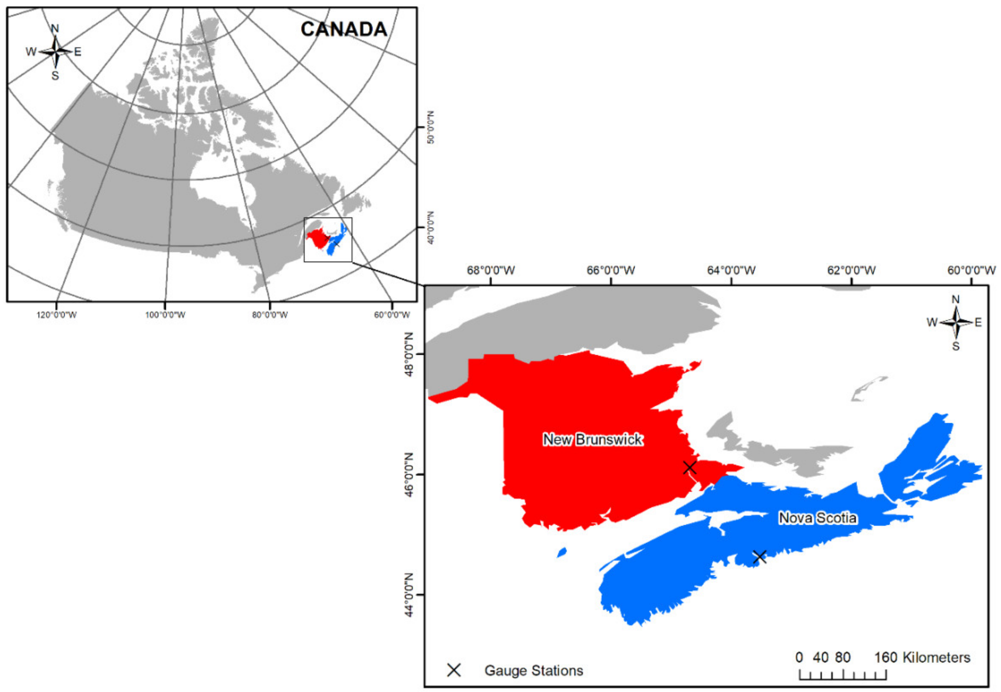
2. Study Area and Data Used

Since this study aims to analyze the impact of non-stationarity on IDF curves under climate change, the case study area is selected based on the presence of non-stationary behavior in the observed rainfall data. The proposed methodology is implemented with the annual maximum rainfall series at two gauging stations located in the Maritime Provinces of Canada: Halifax and Moncton (Figure 1).

Moncton City is located at the Petitcodiac River, area bordered by the Atlantic Ocean, with a maximum height of about 70 m above sea level, and an average precipitation of 1146 mm/year. The Moncton City Köppen–Geiger classification is Dfb (short for a warm-summer humid continental climate [31]), and there is uniform precipitation distribution during the year. Halifax City is bordered by the Atlantic Ocean, lying 8 m above sea level. As Moncton’s, the climate of Halifax is classified as Dfb, with an average precipitation of 1410 mm/year, varying between the drier and colder months. A brief description of the stations used in this study is presented in

Table 1. Stations selected for the study.

Study Area	Station Name	Station ID	Latitude x Longitude	Data Availability
Moncton	Moncton INTL A	8103201	46°7′ N 64°41′ W	1946–2016 (67 years)
Halifax	Shearwater RCS	8205092	46°7′ N 64°41′ W	1955–2016 (59 years)

. Datasets are available through the Environment and Climate Change Canada. Series of 5 min, 10 min, 15 min, 30 min, 1 h, 2 h, 6 h, 12 h and 24 h duration rainfall can be downloaded from https://climate.weather.gc.ca/prods_servs/engineering_e.html (accessed on 15 November 2020) for the available period.

For this study, precipitation data is derived from 24 GCMs produced for Coupled Model Intercomparison Project Phase 5 (CMIP5) [2] (

Table 2. Global Climate Models (GCM) models used in this study.

Model	Country	Centre Name	Spatial Resolution (Longitude vs. Latitude)
bcc-csm1-1	China	Beijing Climate Center, China Meteorological Administration	2.8 × 2.8
bcc-csm1-1-m	China	Beijing Climate Center, China Meteorological Administration	2.8 × 2.8
BNU-ESM	China	College of Global Change and Earth System Science	2.8 × 2.8
CanESM2	Canada	Canadian Centre for Climate Modeling and Analysis	2.8 × 2.8
CCSM4	USA	National Center of Atmospheric Research	1.25 × 0.94
CESM1-CAM5	USA	National Center of Atmospheric Research	1.25 × 0.94
CNRM-CM5	France	Centre National de Recherches Meteorologiques and Centre Europeen de Recherches et de Formation Avancee en Calcul Scientifique	1.4 × 1.4
CSIRO-Mk3-6-0	Australia	Australian Commonwealth Scientific and Industrial Research Organization in collaboration with the Queensland Climate Change Centre of Excellence	1.8 × 1.8
FGOALS-g2	China	IAP (Institute of Atmospheric Physics, Chinese Academy of Sciences, Beijing, China) and THU (Tsinghua University)	2.55 × 2.48
GFDL-CM3	USA	National Oceanic and Atmospheric Administration’s Geophysical Fluid Dynamic Laboratory	2.5 × 2.0
GFDL-ESM2G	USA	National Oceanic and Atmospheric Administration’s Geophysical Fluid Dynamic Laboratory	2.5 × 2.0
HadGEM2-AO	United Kingdom	Met Office Hadley Centre	1.25 × 1.875
HadGEM2-ES	United Kingdom	Met Office Hadley Centre	1.25 × 1.875
IPSL-CM5A-LR	France	Institut Pierre Simon Laplace	3.75 × 1.8
IPSL-CM5A-MR	France	Institut Pierre Simon Laplace	3.75 × 1.8
MIROC5	Japan	Japan Agency for Marine-Earth Science and Technology	1.41 × 1.41
MIROC-ESM	Japan	Japan Agency for Marine-Earth Science and Technology	2.8 × 2.8
MIROC-ESM-CHEM	Japan	Japan Agency for Marine-Earth Science and Technology	2.8 × 2.8
MPI-ESM-LR	Germany	Max Planck Institute for Meteorology	1.88 × 1.87
MPI-ESM-MR	Germany	Max Planck Institute for Meteorology	1.88 × 1.87
MRI-CGCM3	Japan	Meteorological Research Institute	1.1 × 1.1
NorESM1-M	Norway	Norwegian Climate Center	2.5 × 1.9
NorESM1-ME	Norway	Norwegian Climate Center	2.5 × 1.9
GFDL-ESM2M	USA	National Oceanic and Atmospheric Administration’s Geophysical Fluid Dynamic Laboratory	2.5 × 2.0

). These data are bias corrected and statistically downscaled GCM projections generated using the Bias Correction Constructed Analogues with quantile (version 2) mapping reordering (BCCAQv2) for Canada, at a gridded resolution of 300 arc-seconds (0.0833 degrees, or roughly 10 km) for the simulated period of 1950–2100 [32]. BCCAQv2 corrects the bias in daily precipitation series obtained from climate models so the distribution properties are close to historical [33,34]. The climate models were selected based on the availability of precipitation projections for different RCP scenarios (2.6, 4.5 and 8.5). The data used in the study is available from the Pacific Climate Impacts Consortium (PCIC) website (https://data.pacificclimate.org/portal/downscaled_gcms/map/, accessed on 1 July 2020).

3. Methodology

The presented methodology is based on a modification of the EQM method, originally developed by [11] and updated by [24]. The EQM method is currently used for updating the IDF curves under climate change without consideration of non-stationarity modelling [32]. The methodology proposed in this paper extends EQM by addressing the non-stationary behavior of rainfall into the generation of IDFs under the climate change. The proposed methodology is named EQM_NS and is schematically shown in Figure 2.

The EQM_NS methodology includes:

• Statistical analysis: applied to fit stationary and non-stationary probability distributions to both historical and future projected data. An information criteria method is used to identify the best probability distribution model, and a significance test is performed to assess the statistical significance of the non-stationary model in comparison to the stationary one;
• Updating IDF curves for future conditions (EQM_NS): a modified EQM methodology is applied to generate future sub-daily annual maximum precipitation data, and update IDF curves for future period under non-stationary conditions.

3.1. Statistical Analysis

The following discussion provides a detailed description of the statistical analysis implemented in this study.

3.1.1. Theoretical Probability Distribution

Extreme events are usually modelled using peaks-over threshold (POT) and block maxima [35]. The first fits all events exceeding a specific threshold to a generalized Pareto distribution (GP) and the occurrence of an exceedance to a Poisson process. Block maxima consists on fitting a theoretical probability distribution to blocks of annual maximum precipitation values. Both approaches are widely used in extreme events studies (see [5]); however, the implementation of the POT approach involves subjective choices regarding the specification of the threshold, decluttering of threshold exceedances and the treatment of the annual cycle [36]. Furthermore, the availability of data on extremes is often processed into block maxima, which do not allow POT analysis, such as the Environment Canada data, used in this study.

Let the time series, denoted by {x₁,x₂,…,x_n}, be independent and identically distributed (i.i.d.) with common cumulative distribution function. The annual maximum series can be approximate to a theoretical probability of extremes (e.g., GEV, Gumbel, Fréchet, Weibull). In fact, GEV probability distribution is a family of three distributions combined into one: Gumbel, Fréchet and Weibull. GEV distribution is applied by many studies of extreme precipitation [5,6,32,37,38]. The GEV cumulative distribution function F(x) is given by Equation (1) for ξ ≠ 0 [35]:

$$F\left(x/\mu ;\sigma ;\xi \right)=\left\{\begin{array}{c}\exp \left\{-{\left[1+\frac{\xi \left(x-\mu \right)}{\sigma }\right]}^{-1/\xi }\right\},\sigma >0.1+ \frac{\xi \left(x-\mu \right)}{\sigma },\xi \ne 0 \\ \exp \left\{-\exp \left[-\frac{\left(x-\mu \right)}{\sigma }\right]\right\},\sigma >0,\xi =0 \end{array}\right.$$

(1)

where μ is the location parameter, which describes the shift of a distribution, σ is the scale parameter, describing the spread of the distribution, and ξ is the shape parameter, which describes the tail behavior and directly estimated values of extreme precipitation [39]. ξ > 0 represents the heavy-tailed Frechét case, and its probability density function decreases at so slow a rate in the upper tail; ξ = 0 gives the light-tailed Gumbel case, representing an unbounded tail; and ξ < 0 the short-tailed Weibull case, where the distribution has a bounded upper tail [40].

Based on the Extreme Value Theory (EVT) advancements, the non-stationary behavior can be introduced in GEV model by expressing one or more of the parameters as functions with a covariate. In this study, time is used as a covariate for developing non-stationary IDF curves. Empirical studies indicate that it is preferable to represent the non-stationarity in both location and scale parameters [41]. The shape parameter is usually difficult to estimate accurately-it is unrealistic to try modeling ξ as a smooth function of time [35].

Table 3. List of Generalized Extreme Value (GEV) models used in this study and their parameter combinations. $\mu ,\sigma ,$ and $\xi$ are the GEV parameters and ‘t’ is the scoring year for which maximum is taken.

GEV Model
ID	Specification
I	F ($\mu ;\sigma ;\xi )$
II	F (${\mu }_0+{\mu }_1\mathrm{t};\sigma ;\xi )$
III	F (${\mu }_0+{\mu }_1\mathrm{t};{\sigma }_0+{\sigma }_1\mathrm{t};\xi )$
IV	F (${\mu }_0+{\mu }_1\mathrm{t};e^{\left(\sigma 0+\sigma 1\mathrm{t}\right)}$;$\xi )$
V	F ($\mu ;{\sigma }_0+{\sigma }_1\mathrm{t};\xi )$
VI	F ($\mu ;e^{\left(\sigma 0+\sigma 1\mathrm{t}\right)};\xi )$
VII	F (${\mu }_0+{\mu }_1\mathrm{t}+{\mu }_2{\mathrm{t}}^2;\sigma ;\xi )$
VIII	F (${\mu }_0+{\mu }_1\mathrm{t}+{\mu }_2{\mathrm{t}}^2;{\sigma }_0+{\sigma }_1\mathrm{t};\xi )$
IX	F (${\mu }_0+{\mu }_1\mathrm{t}+{\mu }_2{\mathrm{t}}^2;e^{\left(\sigma 0+\sigma 1\mathrm{t}\right)};\xi )$

presents nine models used in this study (eight non-stationary and one stationary).

Different functions can be considered to represent the parameters’ behavior. Here, nine GEV models are constructed using one stationary GEV model (I) and eight non-stationary GEV models (II–IX), based on combinations of trends in both location and/or scale parameters. GEV-I is expressed as a stationary model, with all parameters kept constant; GEV-II to GEV-IX models are non-stationary models, with location parameter conditioned to be a linear or polynomial function of time, and scale parameter assumed to be linear or exponential function of time, while keeping the shape parameter constant. These functions are commonly found in hydrological and climate change studies when investigating trends in distribution model parameters [14,26,42,43], although linear and log-linear models are usually preferred [42].

Estimating GEV parameters is not a simple procedure since it may require complex calculations. The maximum likelihood estimator (MLE) is considered one of the most efficient methods for this estimation [41,44], and can be easily extended to the non-stationary case [45]. Therefore, in this study, MLE is used to estimate the parameters of the GEV distribution. For the annual maximum series X = {x₁,x₂,…,x_n} with n years, the log-likelihood derived from Equation (1) is given by Equation (2), for the stationary case.

For ξ ≠ 0,

$$\begin{array}{ll}logL\left(X;\mu ;\sigma ;\xi \right)=& -n\log \sigma \\ & -\left(1+\frac{1}{\xi }\right){\displaystyle {\displaystyle \sum }_{i=1}^n}\log \left[1+\frac{\xi \left(x_i-\mu \right)}{\sigma }\right]-{\displaystyle {\displaystyle \sum }_{i=1}^n}{\left[1+\frac{\xi \left(x_i-\mu \right)}{\sigma }\right]}^{-1/\xi },1\\ & +\frac{\xi \left(x_i-\mu \right)}{\sigma }>0\end{array}$$

(2)

Instead of a direct maximization method, MLE estimator commonly uses the minimization of the negative log-likelihood, as provided by Equation (2). It is important to notice that Equation (2) is formulated for GEV family with ξ ≠ 0, disregarding the Gumbel distribution. For the non-stationary cases, the location and scale parameters in the Equations (1) and (2) are replaced in accordance with the non-stationary setting presented in Table 3. Given the requirements of iterative numerical procedures to solve the function, RStudio extRemes package (version 2.0-10) is used to fit GEV parameters to data based on MLE estimator for the stationary and non-stationary cases [46]. The MLE method can even be useful for selecting the best GEV model, which provides an efficient procedure for the development of rainfall quantiles.

3.1.2. Identification of the Best Model

Akaike’s Information Criteria (AIC) is a common method for selecting the best GEV model among all candidates [45]. It penalizes the minimized negative log-likelihood function ($-logL$) for the number of parameters estimated for each model. However, depending on the relation between the sample size n and the number of parameters k presented in practical applications, the Corrected Akaike’s Information Criteria (AICc) is recommended (n/k > 40) because it helps to avoid overfitting the data. AICc converges to AIC for large n [47]. From a collection of nested candidate models with k parameters, fitted to an annual maximum rainfall series with a sample size of n, AIC and AICc are expressed by Equations (3) and (4), respectively:

$$AIC\left(k\right)=-2logL+2k$$

(3)

$$AICc\left(k\right)=AIC\left(k\right)+\frac{2k\left(k+1\right)}{n-k-1}$$

(4)

where k is the number of parameters of a specific model. AICc values are much more affected by the sample size of the data series, so the rescaled form of AICc, ${\mathsf{\Delta }}_i$ is used to rank the GEV models as given by Equation (5):

$${∆}_i=AICc-\min \left(AICc\right)$$

(5)

where min(AICc) is the smallest AICc among all the models. The model which has ${∆}_i$ value zero is the best model and the models having ${∆}_i \le 2$ as reasonably good choices [47].

When a non-stationary model is identified as the best GEV model, it is necessary to assess its statistical significance against the stationary GEV model. The best non-stationary model’s significance can be checked by the likelihood ratio test (LR-test), usually recommended when comparing two candidate models. The test of the null hypothesis of no trend (stationary model) can be performed by comparing the minimized negative log-likelihood functions of the stationary and the best non-stationary model [45] (Equation (6)):

$$-log{L}_s\times -log{L}_{ns}$$

(6)

where $-log{L}_s$ is the negative log-likelihood of the stationary model, and $-log{L}_{ns}$ is the negative log-likelihood of the best non-stationary model.

Under the null hypothesis of no trend, the likelihood ratio test statistic, based on twice the difference between $-log{L}_s$ and $-log{L}_{ns}$, has an approximate Chi squared distribution (${\chi }^2$) where the degree of freedom is denoted as the difference between the number of parameters of the models [46]. The LR statistic is given by Equation (7):

$$D=2\left[-log{L}_s+log{L}_{ns}\right]~{\chi }^2$$

(7)

The statistical significance of the best non-stationary model, when compared to the stationary model, can be measured from the p-value of Chi-square distribution [6]. In this study, if the p-value is lower than the 0.05 (95% confidence level), the best non-stationary model is statistically significant compared to the stationary model.

3.1.3. Rainfall Depth Estimation

The inverse distribution function is used to estimate the rainfall depth, based on the conventional T-year return period (1/(1−F)). For stationary GEV model and ξ ≠ 0, the rainfall intensity z_p is given by Equation (8):

$$z_p=\mu -\frac{\sigma }{\xi }\left[1-\left\{-\ln {\left(1-\frac{1}{T}\right)}^{-\xi }\right\}\right]$$

(8)

However, once the best GEV model is identified as non-stationary, its location and/or scale parameter value vary over the time. Thus, the time-variant parameters are derived by computing the 95th percentile of the trending parameter’s value by Equations (9) and (10), under a low risk approach [37]. The calculated model parameters are then replaced in Equation (8) and non-stationary rainfall intensity or rainfall depth is estimated.

$${\widehat{\mu }}_{95}=Q_{95}\left({\widehat{\mu }}_1,{\widehat{\mu }}_2,\dots ,{\widehat{\mu }}_n\right)$$

(9)

$${\widehat{\sigma }}_{95}=Q_{95}\left({\widehat{\sigma }}_1,{\widehat{\sigma }}_2,\dots ,{\widehat{\sigma }}_n\right)$$

(10)

Ultimately, there are several formulations for adjusting IDFs in the form of smoothing curves [43]. In this paper, the general formulation used is shown in Equation (11):

$$I=A{\left(d+C\right)}^B$$

(11)

where I is the rainfall intensity (mm/h); A, B and C are the coefficients for each return period (T) in years; and d is the duration of precipitation in hours.

3.2. Non-Stationary IDF Curves under Changing Climate

A modified EQM method generates non-stationary IDF curves under changing climate conditions (EQM_NS). EQM method captures the distribution of changes between the projected time period and the baseline period (temporal downscaling) in addition to spatial downscaling of the annual maximum precipitation derived from the GCM data and the observed sub-daily data [11].

In original EQM, the quantile-mapping function performs the spatial downscaling by transferring the quantile of the historically observed distribution to the historically modeled distribution [20]. This method is highly recommended to be used for IDF purposes, since it allows the application of annual maximum precipitation from climate model simulated rainfall [14,48] instead of using complete daily precipitation records [29]. Using the principle of quantile mapping, the cumulative probability distribution of the GCM ($F_{m,h}$) and the sub-daily series ($x_{j,o,h}$) are equated to establish a statistical relationship between them and to obtain GCM modeled sub-daily (${\widehat{x}}_{j,o,h}$) values as shown in Equation (12):

$${\hat{x}}_{j,o,h}=F_{j,o,h}^{-1}\left[F_{m,h}\left(x_{m,h}\right)\right]$$

(12)

where $\hat{x}$ is the annual maximum quantile at the station scale, F is the cumulative distribution functions and $F^{-1}$ is its inverse. j,o,h correspond to each sub-daily (‘j’) observed rainfall data (‘o’) in historical-baseline period (‘h’), while ‘m’ remains the modeled data. The quantiles extracted from each pair ${\hat{x}}_{j,o,h}$ and $x_{m,h}$ are equated to establish a functional relationship in the form of the Equation (13).

$${\hat{x}}_{j,o,h}=\frac{a_j+x_{m,h}}{b_j+c_j{x}_{m,h}}+\frac{d_j}{x_{m,h}}$$

(13)

where $a_j,b_j,c_j$ and $d_j$ are the adjusted coefficients. A Differential Evolution optimization algorithm [49] is used to fit the coefficients. The Ordinary Least Squares method is used as the objective function to be optimized (minimized) in order to obtain the optimal set of coefficients. Unlike the original EQM, in which spatial downscaling is applied assuming no trend pattern in GEV distribution parameters of historic period, the new EQM_NS introduces the effects of non-stationarity in historic AMPs time series by adopting the 95th percentile values from the varying parameter(s) (Equations (9) and (10)) in Equation (12). This step ensures that the non-stationarity presented even in the historic period is accounted for generating IDFs for future conditions.

The second step of EQM algorithm is the temporal downscaling, which finds the relationship between GCM daily maximum precipitation for the baseline period and the future GCM-simulated (for all RCPs) daily maximum precipitation [11]. Similar to EQM, EQM_NS uses the quantile delta mapping, since it preserves the relative changes in the precipitation mean and quantiles obtained from the climate models [24,50]. The cumulative probability distribution of the GCM generated rainfall in the future period ($F_{m,f}$) and the GCM generated rainfall in the baseline period ($x_{m,h}$) are equated to establish a statistical relationship (Equation (14)). In addition, the relative change between the historical and future period is given by Equation (15):

$${\hat{x}}_{m,h}=F^{-1}{}_{m,h}\left[F_{m,f}\left(x_{m,f}\right)\right]$$

(14)

$${∆}_m=\frac{x_{m,f}}{{\hat{x}}_{m,h}}$$

(15)

where m,f corresponds to the modeled data (‘m’) in future projection period (‘f’), and ${∆}_m$ is the relative change. Projected future maximum sub-daily series ($x_{j,f}$)) at the station scale is then generated using Equation (13) by replacing $x_{m,h}$ with ${\hat{x}}_{m,h}$ and multiplying it by the relative change ${∆}_m$ from Equation (15) as given by Equation (16):

$$x_{j,f}={∆}_m·{\widehat{x}}_{j,o,h}$$

(16)

Future IDF curves are generated by repeating the statistical analysis presented in Section 3.1 (Equations (1)–(11)), given the future sub-daily time series. The application of these analysis is necessary since they certify the presence of non-stationarity in future sub-daily series and estimation of future non-stationary rainfall intensity.

4. Results and Discussions

In order to evaluate the proposed methodology, this study used the precipitation series of 5 min, 10 min, 15 min, 30 min, 1 h, 2 h, 6 h, 12 h and 24 h durations available for the selected stations. Section 4.1 provides an overview of extreme precipitation for Moncton and Shearwater stations, pointing towards the best GEV modeling for sub-daily observed data, while its effect is presented in the form of rainfall intensity in Section 4.2. Section 4.3 analyzed the new conditions for spatial downscaling to ensure the formulation of Equation (12) is able to establish a statistical relationship between the quantiles from observed and GCM series for the historical baseline period. This analysis is presented using the multimodel ensemble median of the 24 GCMs. Future IDFs are developed for 2-, 5-, 10-, 25-, 50- and 100-year return periods, which are commonly used in water infrastructure design and management. We presented the uncertainty introduced by different GCM model in rainfall depths estimation. Based on the multimodel ensemble median, future IDF curves are analyzed, which includes: (i) changes in the stationary future rainfall intensities compared to the observed rainfall intensities (EQM); (ii) changes in the non-stationary future rainfall intensities compared to the observed rainfall intensities (EQM_NS); and (iii) differences between the future rainfall intensities, obtained using stationary and non-stationary conditions.

The EQM_NS methodology implementation is done using the open-access RStudio programming environment [51], based on its available packages and functions [52].

4.1. Trends in GEV Model Parameters in Historical Observed Data

Nine GEV models are used to identify and analyze trends in the annual maximum rainfall distribution parameters for both gauging stations. As presented in Tables S1 and S2 (Supplementary Material) for Moncton and Shearwater stations, respectively, the results indicate a presence of non-stationarity for some durations, based on the existence of trends in GEV parameters.

For Moncton station, results indicate a significant trend pattern in GEV’s location or scale parameters among rainfall durations. GEV-I is not ranked as best, except for short rainfall durations (5- and 10-min). On the other hand, GEV-II is the only model that has substantial support to be a candidate model for all durations with ${∆}_i$ ≤ 2 [48]. In other words, there is a trend in the location parameter in extreme precipitation. Further, for all durations, GEV-VIII and GEV-IX models did not appear as a reasonable choice based on ${∆}_i$ value. For 5 and 10 min, the GEV-I is found to be the best GEV model (the GEV parameters remain constant). For 15 and 30 min, GEV-VI and GEV-V are identified as the best, respectively, representing a trend in scale parameter (increase indicates a higher spread of distribution over the years). Otherwise, for durations greater than 1 h a trend in location parameter is found to be the best choice model, with GEV-II for 1, 6 and 12 h and GEV-VII for 2 h.

Unlike the Moncton station, most of the durations at Shearwater station can be considered stationary based on the ${∆}_i$ value, except for 1440 min in which a linear trend in the location parameter (GEV-II) is statistically significant. For 360 min, a linear trend in the scale parameter (GEV-V) is given as the best model. It can be observed in Table S2 that, for most all the durations GEV-II model is a reasonable choice for Shearwater Station, with exceptions of 10 and 15 min.

The best GEV model identified by Table S1 supports the estimative of GEV parameters as presented in

Table 4. Parameters of GEV distribution, in mm, for historical data for the Moncton station.

Duration (Minutes)	Best GEV-Type	Stationary GEV Model			Best GEV Model (95th Percentile)			LR-Test (p-Value)
		Location	Scale	Shape	Location	Scale	Shape
5	I	5.18	2.10	0.07	5.18	2.10	0.07	-
10	I	7.32	2.92	0.07	7.32	2.92	0.07	-
15	VI	8.92	3.35	0.09	9.01	4.27	0.14	0.043
30	V	12.03	4.12	0.08	12.33	5.51	0.06	0.030
60	II	16.22	4.60	0.22	18.06	4.10	0.31	0.011
120	VII	22.22	5.63	0.23	25.46	5.19	0.30	0.047
360	II	35.30	11.07	−0.02	39.97	10.78	−0.03	0.041
720	II	43.59	14.35	0.02	50.68	13.86	0.004	0.016
1440	II	51.44	17.45	0.05	61.62	15.95	0.08	0.002

, whereas best GEV model of Table S2 supports the results of

Table 5. Parameters of GEV distribution, in mm, for historical data for the Shearwater station.

Duration (Minutes)	Best GEV-Type	Stationary GEV Model			Best GEV Model (95th Percentile)			LR Test (p-Value)
		Location	Scale	Shape	Location	Scale	Shape
5	I	4.98	1.46	0.07	4.98	1.46	0.07	-
10	I	7.67	2.16	0.001	7.67	2.16	0.001	-
15	I	9.88	2.80	−0.13	9.88	2.80	−0.13	-
30	I	13.88	3.95	−0.16	13.88	3.95	−0.16	-
60	I	19.17	4.94	−0.06	19.17	4.94	−0.06	-
120	I	26.30	6.95	0.04	26.30	6.95	0.04	-
360	V	44.24	11.94	−0.004	43.93	14.67	0.14	0.044
720	I	54.57	14.34	−0.06	54.57	14.34	−0.06	-
1440	II	60.59	16.05	0.08	66.61	15.05	0.12	0.030

. Although a single model for all durations is often assumed, these parameters are calculated based on the best model fitted to each duration data. For all the identified non-stationary models, there is upward trend in the varying parameters, indicating an underestimation of values in the stationary GEV model, and further, the rainfall depth estimation. AICc values for a specific duration do not show great variations. The same is found for ${∆}_i$ values, which indicates how sensitive these results can be when the same covariate is considered. In addition, GEV-VIII and GEV-IX have the highest AICc values for most of all the durations, indicating that they are not to be used for non-stationary modelling at the selected stations.

Overall, it is important to verify if the estimates for GEV parameters are reasonable, especially the shape parameter, since it directly influences the tails of the distribution [25]. The shape parameter value is in the range of −0.16 to +0.31, which is in line with the findings of [38] for daily time series stationary analysis for the specific study region. In this way, these results are suitable to be incorporated into the GCM data bias-correction.

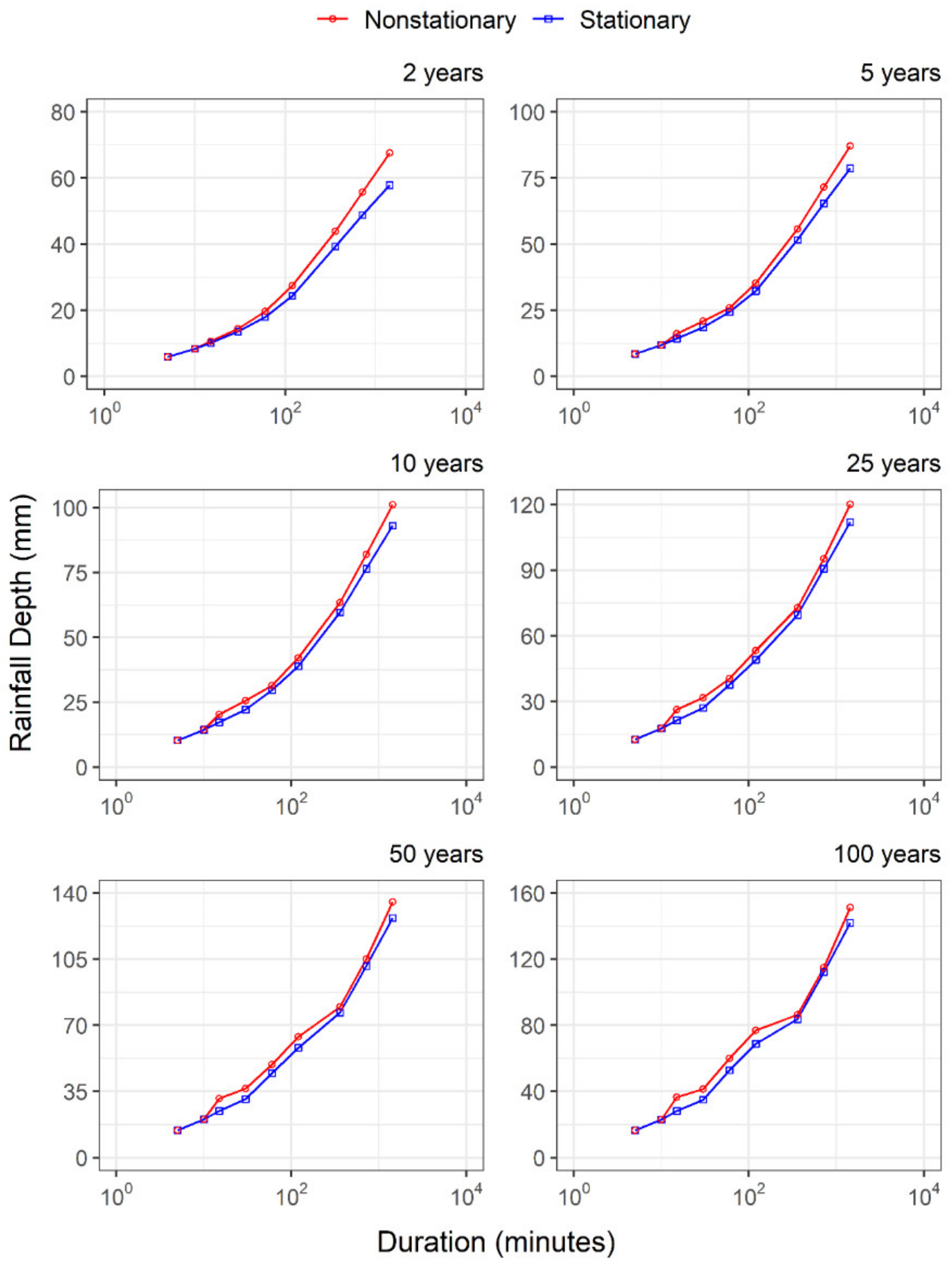
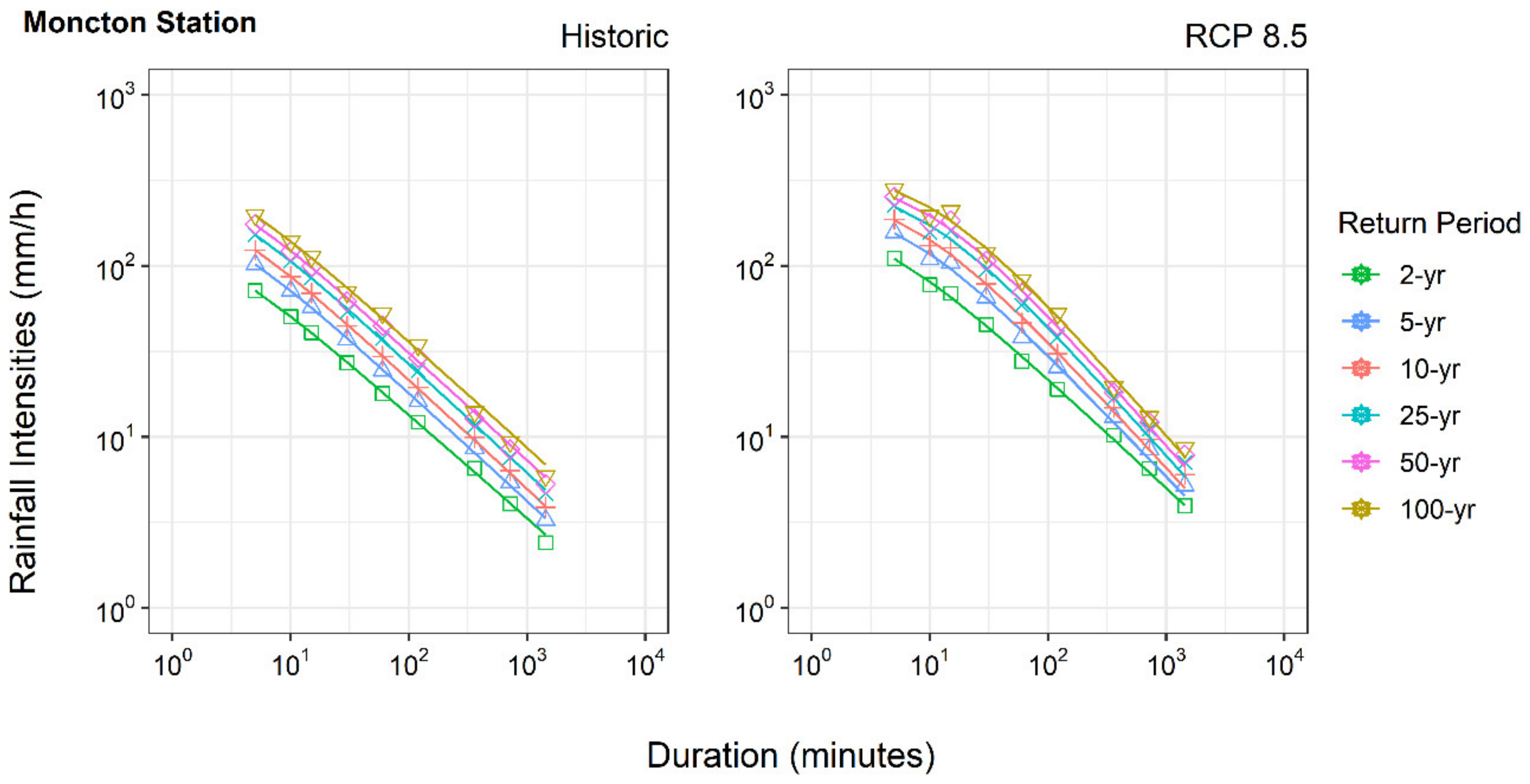
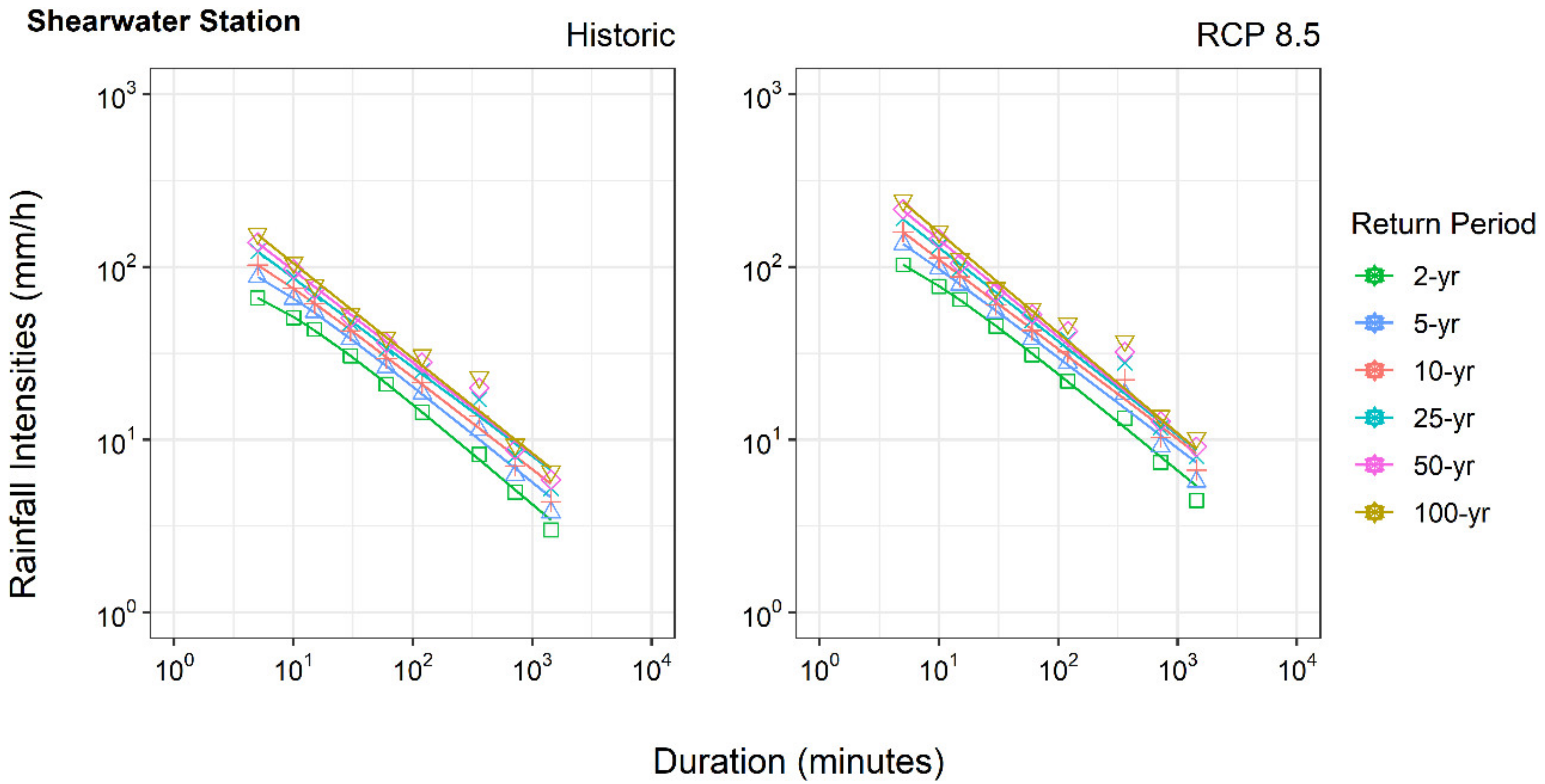
4.2. Historic IDF Relationships

Based on the best-fitted GEV models for different durations of the observed data for Moncton and Shearwater stations, IDF relationships for 2-, 5-, 10-, 25-, 50- and 100-year return periods are developed using Equation (8) (Figure 3 and Figure 4). In addition, for comparison purposes, the IDFs for the stationary case (GEV-I) are also developed. This comparison provides some additional insights about the observed historical period. Overall, non-stationary IDFs differ for different durations and therefore the observed differences and relative changes (i.e., the percentual value of rainfall increment provided by the non-stationary model compared with the stationary model) do not follow a similar pattern. Therefore, given the different trends over durations, there are some cases in which rainfall depth for a lower duration appears as superior to the rainfall intensity for a higher duration (e.g., in Figure 4, the rainfall depth estimated for 360-min and 25-year is higher than the rainfall depth estimated for 720-min and same return period). These results are expected since the trend parameters are assessed for each duration, assuming an independence assumption [43]. In addition, the rainfall depth presented here is estimated using the inverse of GEV function which parameters’ behavior varies according to its assessed performance. Further, even being in the same geographic region, the difference in the observed time period between stations may lead to different trends associated with data (as the assessed GEV models indicated), and further to the estimated rainfall quantiles. Also, the type of the covariate used, i.e., time, may lead to different trends, while large-scale variables may produce more convergent results for the same climatic region [6].

The relative changes vary with the non-stationary GEV model for calculated IDF relationships among different durations. On one hand, for those durations in which non-stationary GEV model shows a trend in the location parameter, there is no observable pattern of relative change among different return periods. The relative change is higher for low durations and lower for high durations among durations. On the other hand, when the non-stationary GEV model of a trend in the scale parameter is considered, the relative change increases with the rainfall duration. For Moncton station, relative changes for 100-year return period is about 29.9% for 15-min duration (when there is a trend in the scale parameter) and 6.5% for 1440 min (when there is a trend in the location parameter). This trend condition results in 40.2% (360-min) values and 6.4% (1440-min), respectively, for the Shearwater station.

The results provided indicate that, for both minor and major significant water infrastructure systems, the difference between stationary and non-stationary rainfall intensities can be very significant in terms of design and operations. Furthermore, even in flood mapping, usually produced with higher return periods, underestimating extreme precipitation events can lead to underestimated flow values.

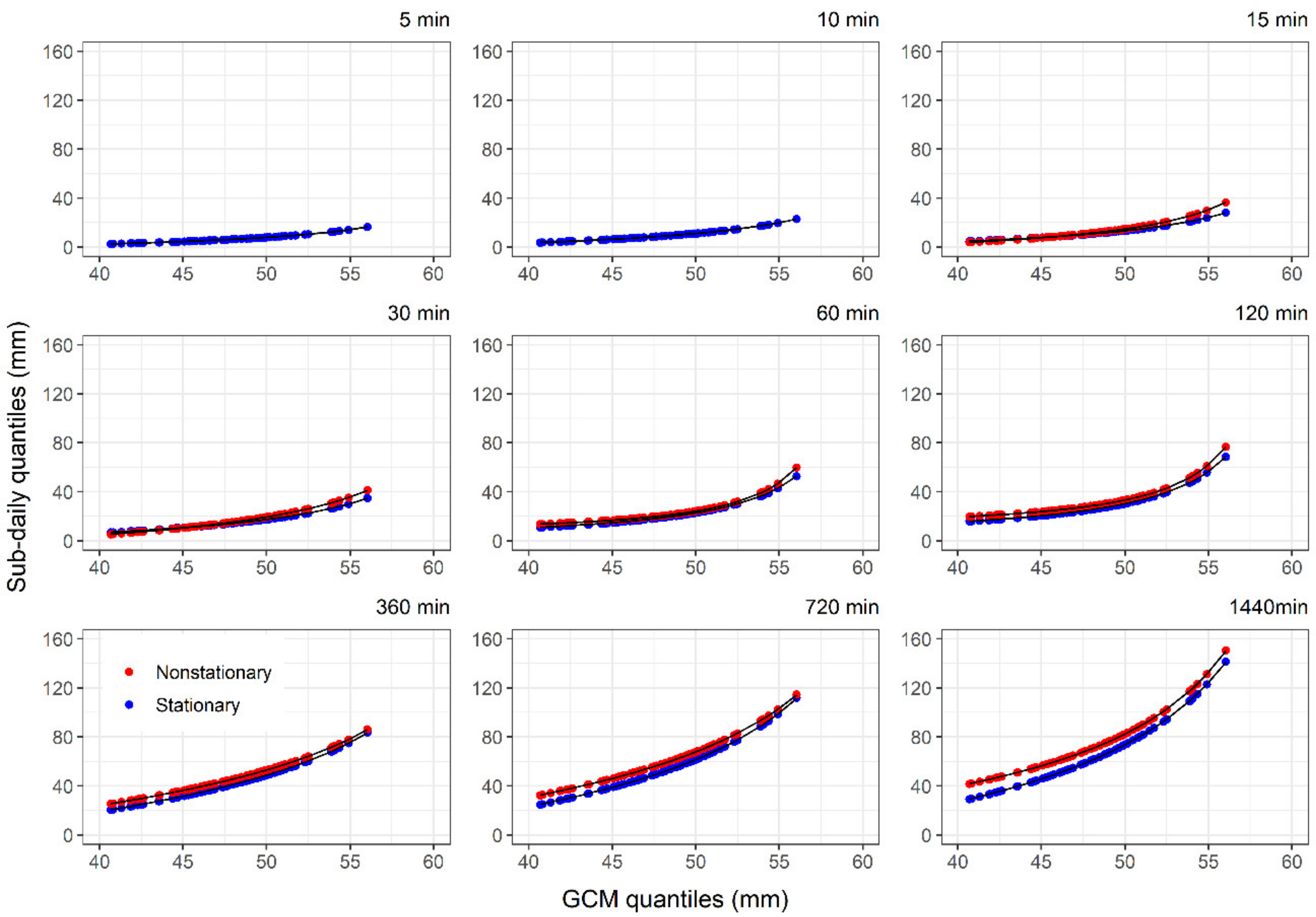
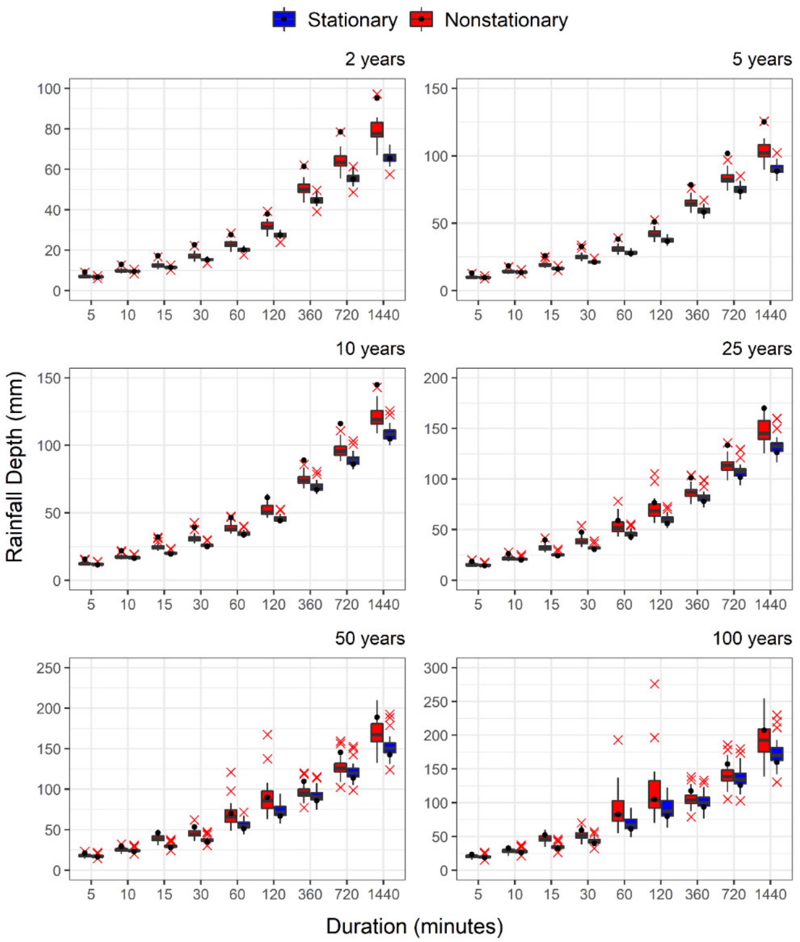
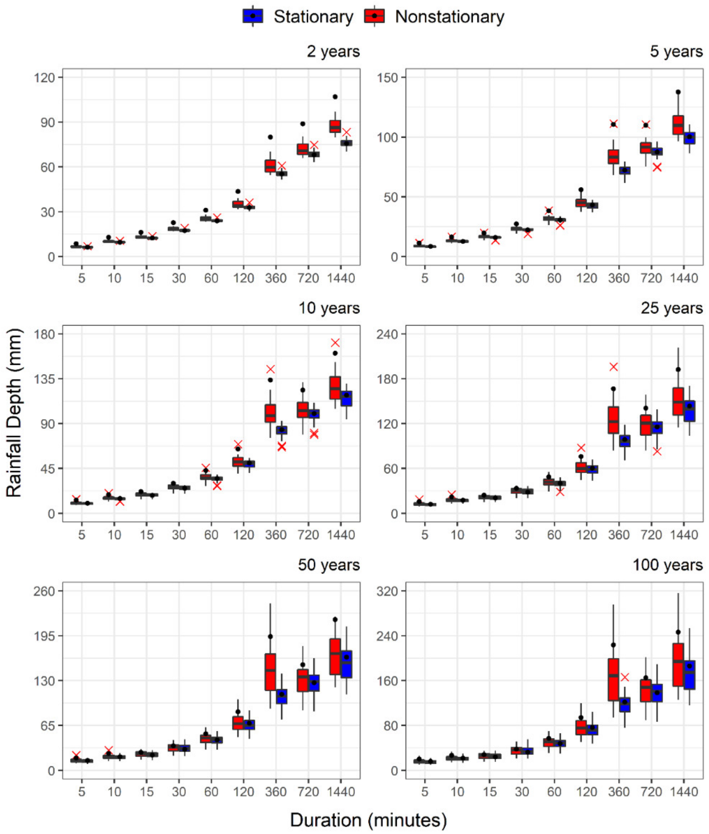
4.3. Performance of the Modified Spatial Downscaling

In this section, the location and/or scale parameters’ 95th percentile is computed based on the best GEV model and used to find a statistical relationship between observed and GCM modeled data for historical-baseline period, obtained in the form of a non-linear regression (Equation (13)). This is the modification adopted in the spatial downscaling to transfer the effects of non-stationarity in the observed period to future IDFs.

AMP quantiles at the station scale are presented in Figure 5, given the ensemble median performance. Figure 5 presents a comparison of stationary and non-stationary values, for those durations where the non-stationary behavior is identified. The results suggest larger quantile values for non-stationary conditions in comparison with stationary condition, with exception of low quantiles for short durations (e.g., less than 30-min duration). A similar quantile’s ascendance is identified between GEV modeling conditions, and the differences are greater for high rainfall durations. In addition, non-linear regression curve is presented, ensuring that the format is adequate to represent the relationship between sub-daily and GCM based historical data. Thus, results confirm that the adoption of non-stationarity in observed data in spatial downscaling is able to embed the effects of identified trends.

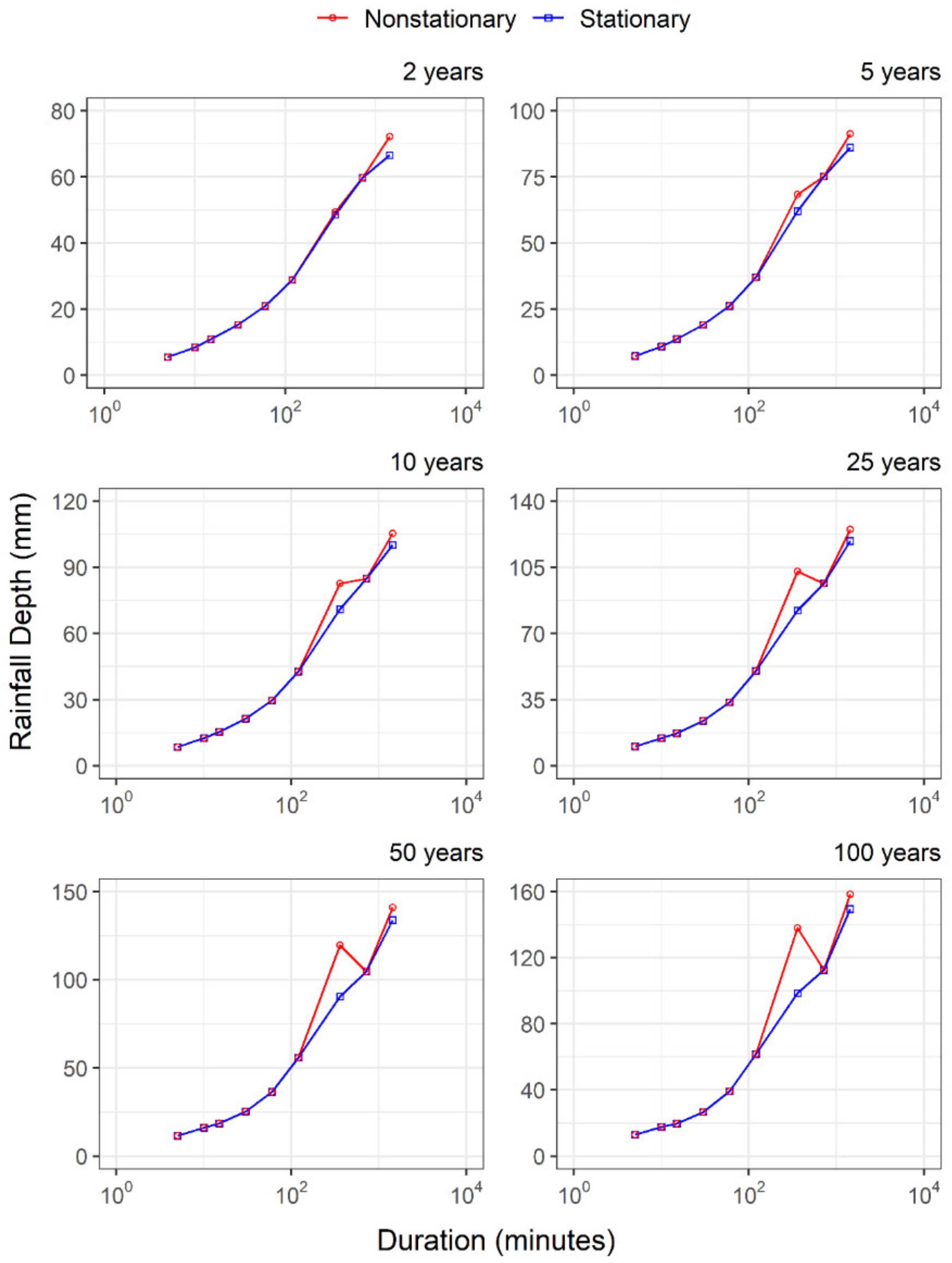
4.4. Future IDF Curves

Future rainfall depth estimation using all GCM datasets is presented in Figure 6 and Figure 7, for Moncton and Shearwater stations, respectively, and for the RCP 8.5 projection scenario. Other scenarios are available in the Supplementary Material (Figures S1 to S4). The boxplot graph shows how uncertainty on estimated rainfall quantiles is inherent to the choice of a single GCM. Overall, it is observed that the variation increases with rainfall duration and return period. These uncertainties are higher for non-stationary behavior than for the stationary, which is expected since the behavior of future sub-daily time series depends on the GCM model and is influenced by the identified best fitted GEV model.

Rainfall depth estimated using the multimodel median ensemble of the 24 GCMs is also presented in Figure 6 and Figure 7. Note that the median ensemble is obtained as the median value of AMPs outputs for each GCM model, and its rainfall depth as result does not necessarily represent the median of results from all the GCM models generated by the boxplot graph. In spite of the observed outliers, results from the ensemble can represent the rainfall depth for different future projections, being able to supply the several variables incorporated for different single models. Table S3 shows the GEV parameters fitted according to the best GEV model statistically defined for each duration and RCP 8.5 scenario for Moncton station, whereas Table S4 presents results for Shearwater station.

IDF curves generated based on the ensemble of 24 GCMs for the RCP 8.5 scenario (up to 2100) are presented in Figure 8 and Figure 9 for both gauging stations (see Figures S5 and S6 in the Supplementary Material for other RCPs). The IDF curves for the historical period are included allowing the comparison of the periods. In general, the curves shift upward from the historical period to future period. There is an increase in the future precipitation intensities, for all return periods and durations, and for both the stationary and non-stationary scenarios, although with different magnitudes. The degree of rainfall increase varies and depends on duration (on how the time series is modelling). These findings suggest that future extreme rainfall events will exceed the capacity for which the current water infrastructure is designed, pointing out the need for updating IDF curves. Regarding the RCP scenarios, the rainfall increase does not follow the severity of the scenario, which can be internally related to the nature of data and climate model used in the analysis.

Completed results can be observed in the Supplementary Material (Tables S5 and S6). The following observations are made based on the results of the analysis. Considering all the RCP scenarios, when comparing the observed stationary (S) with future non-stationary (NS) rainfall intensities, it is found that the increase is higher for those durations that present increasing trend patterns, even in the present period. For example, higher changes are observed for 360 min at Shearwater, compared to 60 min at Moncton. The results suggest that a trend pattern in the scale parameter of time series greatly influences the rainfall intensities, and this behavior is translated to the future period. For the RCP 4.5 and RCP 8.5 scenarios, the comparison of rainfall intensities from observed S and future S (from EQM) presents increasing pattern for different return periods. At Moncton station, the relative change is reduced with the increase of return period, whereas the opposite behavior is observed at Shearwater station. In spite of a higher increase, when comparing observed S and future NS rainfall intensities, a similar behavior is found at both stations. For those durations with observed scale parameter trends in the historical period (e.g., 15 min in Moncton and 360 min in Shearwater), the increase is much more significant than for other durations. Future NS rainfall intensities are estimated based on the GEV-II model for most of the durations. For the RCP 8.5, the increase up to 64.4% for 2-year return period and up to 55.4% for 100-year return period is observed for Moncton. For Shearwater, these values can reach 59.1% and 65.5%, respectively.

In general, the change imposed by the climate in future is higher for Moncton than for Shearwater, based on the all RCP scenarios, since the degree of change on precipitation is higher for Moncton. The results suggest that return period can be extremely reduced in the future. The magnitude of reduction varies with duration and is much higher under the non-stationary behavior. For example, the observed 100-year return period event of 1440-min duration is 5.9 mm/h, and it is smaller than 6.0 mm/h of the 10-year return period future extreme event for RCP 8.5 scenario at Moncton station. A similar reduction is found for Shearwater station.

5. Summary and Conclusions

This manuscript presents a new methodology that combines non-stationarity and equidistant quantile matching for the development of future IDF curves under climate change conditions. Nine GEV models (one stationary and eight non-stationary) were fitted to the historical data, using time as a covariate in the form of the trend function. Statistical analysis was performed to identify the best GEV model. Once the best GEV model is non-stationary, the trend parameters are used in spatial downscaling for the baseline period. This process ensures that non-stationarity presented in the historical period is considered in generating future rainfall quantiles. A similar procedure is used to verify and quantify future IDF curves. Unlike other methodologies for generating IDF curves under climate change, the methodology presented in this paper is able to consider the non-stationary conditions in the present and future time periods. The proposed methodology is carried out to model the sub-daily precipitation series at the Moncton and Shearwater gauging stations in Canada for the period of 2020 to 2100.

From the observed data, it is noted that non-stationarity is present for most of the durations, indicating a real and current underestimation in water infrastructure planning and design based on the stationary IDF curves. In the future scenario, and compared to the observed IDFs, there is an increase in estimates of rainfall quantiles, which is even more expressive under a non-stationary scenario due to a positive trend presented in the non-stationary modelling. At the same time, the return period reduces with time. This new framework suggests that using non-stationary frameworks to develop future IDF curves is a more conservative approach, being useful in directing ways of change. Otherwise, the magnitude of the change in the future can be highly affected by the model fitted to the data and need to be used with caution, given the complexity and number of uncertainties related to climate simulations.

Given the extended impacts of IDF curves on infrastructure planning and design, we argue for the need in estimating uncertainties arising from different sources, like choice of GCM model or choice of the probability distribution. In this study, the new non-stationary framework is based on the best GEV model. However, the results indicated that the best GEV model may not be non-stationary, and the same non-stationary GEV model may not be the best for all durations. Assessing different non-stationary GEV combinations allows for a broader understanding of the uncertainty in future IDFs introduced through the frequency analyses. Modeling approach used in this study is limited to: (i) one CDF mapping function, i.e., GEV; (ii) one probability distribution parameter estimation, i.e., Maximum Likelihood method; and (iii) the use of one covariate, i.e., time. Other uncertainties are present in climate modeling, especially when dealing with sub-daily durations. Thus, further development of the presented methodology should be carried in order to improve the estimation of future IDFs.

References

1. Mailhot, A.; Duchesne, S. Design criteria of urban drainage infrastructures under climate change. J. Water Resour. Plan. Manag. 2010, 136, 201–208. [Google Scholar] [CrossRef]
2. IPCC. Climate Change 2014: Synthesis Report; Contribution of Working Groups I, II and III to the Fifth Assessment Report of the Intergovernamental Panel on Climate Change; Pachauri, R.K., Meyer, L.A., Eds.; IPCC: Geneva, Switzerland, 2014; 151p. [Google Scholar]
3. Easterling, D.R.; Meehl, G.A.; Parmesan, C.; Changnon, S.A.; Karl, T.R.; Mearns, L.O. Climate extremes: Observations, modeling, and impacts. Science 2000, 289, 2068–2074. [Google Scholar] [CrossRef] [PubMed] [Green Version]
4. Berggren, K. Indicators for Urban Drainage System-Assessment of Climate Change Impacts. In Proceedings of the 11th International Conference on Urban Drainage, Munich, Germany, 31 August–5 September 2008. [Google Scholar]
5. Agilan, V.; Umamahesh, N.V. Detection and attribution of non-stationarity in intensity and frequency of daily and 4-hr extreme rainfall of Hyderabad, India. J. Hydrol. 2015, 530, 677–697. [Google Scholar] [CrossRef]
6. Agilan, V.; Umamahesh, N.V. What are the best covariates for developing non-stationary rainfall Intensity-Duration-Frequency relationship? Adv. Water Resour. 2017, 101, 11–22. [Google Scholar] [CrossRef]
7. Willems, P.; Vrac, M. Statistical precipitation downscaling for small-scale hydrological impact investigations of climate change. J. Hydrol. 2011, 402, 193–205. [Google Scholar] [CrossRef]
8. Nguyen, V.-T.-V.; Nguyen, T.-D.; Cung, A. A statistical approach to downscaling of sub-daily extreme rainfall processes for climate-related impact studies in urban areas. Water Sci. Technol. 2007, 7, 183–192. [Google Scholar] [CrossRef]
9. Hassanzadeh, E.; Nazemi, A.; Elshorbagy, A. Quantile-based downscaling of precipitation using genetic programming: Application to IDF curves in Saskatoon. ASCE J. Hydrol. Eng. 2014, 19, 943–955. [Google Scholar] [CrossRef]
10. Mailhot, A.; Beauregard, I.; Talbot, G.; Caya, D.; Biner, S. Future changes in intense precipitation over Canada assessed from multi-model NARCCAP ensemble simulations. Int. J. Climatol. 2012, 32, 1151–1163. [Google Scholar] [CrossRef]
11. Srivastav, R.K.; Schardong, A.; Simonovic, S.P. Equidistance Quantile Matching Method for Updating IDF Curves under Climate Change. Water Resour. Manag. 2014, 28, 2539–2562. [Google Scholar] [CrossRef]
12. Arnbjerg-Nielsen, K.; Willems, P.; Olsson, J.; Beecham, S.; Pathirana, A.; Gregersen, I.B.; Madsen, H.; Nguyen, V.-T.-V. Impacts of climate change on rainfall extremes and urban drainage system: A review. Water Sci. Technol. 2013, 68, 16–28. [Google Scholar] [CrossRef]
13. Smid, M.; Costa, A.C. Climate projections and downscaling techniques: A discussion for impact studies in urban systems. Int. J. Urban Sci. 2018, 22, 277–307. [Google Scholar] [CrossRef] [Green Version]
14. Ganguli, P.; Coulibaly, P. Assessment of future changes in intensity-duration-frequency curves for Southern Ontario using North American (NA)-CORDEX models with non-stationary methods. J. Hydrol. Reg. Stud. 2019, 22, 100587. [Google Scholar] [CrossRef]
15. Tapiador, F.J.; Navarro, A.; Moreno, R.; Sánchez, J.L.; Gárcia-Ortega, E. Regional climate models: 30 years of dynamical downscaling. Atmos. Res. 2020, 235, 104785. [Google Scholar] [CrossRef]
16. Cannon, A.J.; Innocenti, S. Projected intensification of sub-daily and daily rainfall extremes in convection-permitting climate models simulations over North America: Implications for future intensity-duration-frequency curves. Nat. Hazards Earth Syst. Sci. 2019, 19, 421–440. [Google Scholar] [CrossRef] [Green Version]
17. Prein, A.F.; Rasmussen, R.; Castro, C.L.; Dai, A.; Minder, J. Special issue: Advances in convection-permitting climate modeling. Clim. Dyn. 2020, 55, 1–2. [Google Scholar] [CrossRef] [Green Version]
18. Teutschbein, C.; Seibert, J. Bias correction of regional climate model simulations for hydrological climate-change impact studies: Review and evaluation of different methods. J. Hydrol. 2012, 456–457, 12–29. [Google Scholar] [CrossRef]
19. Sunyer, M.A.; Madsen, H.; Ang, P.H. A comparison of different regional climate models and statistical downscaling methods for extreme rainfall estimation under climate change. Atmos. Res. 2012, 103, 119–128. [Google Scholar] [CrossRef]
20. Maraun, D. Bias correcting climate change simulations—A critical review. Curr. Clim. Change Rep. 2016, 2, 211–220. [Google Scholar] [CrossRef] [Green Version]
21. Herath, S.M.; Sarukkalige, P.R.; Nguyen, V.-T.-V. A spatial temporal downscaling approach to development of IDF relations for Perth airport region in the context of climate change. Hydrol. Sci. J. 2015, 61, 2061–2070. [Google Scholar] [CrossRef] [Green Version]
22. Nguyen, T.-H.; Nguyen, V.-T.-V. Linking climate change to urban storm drainage system design: An innovative approach to modeling of extreme rainfall processes over different spatial and temporal scales. J. Hydroenviron. Res. 2020, 29, 80–95. [Google Scholar] [CrossRef]
23. Bi, E.G.; Gachon, P.; Vrac, M.; Monette, F. Which downscaled rainfall data for climate change impact studies in urban areas? Review of current approaches and trends. Theor. Appl. Climatol. 2017, 127, 685–699. [Google Scholar] [CrossRef]
24. Schardong, A.; Simonovic, S.P.; Sandink, D. Computerized Tool for the Development of Intensity-Duration-Frequency Curves under a Changing Climate: User’s Manual v.3; Water Resources Research Report no. 104; Facility for Intelligent Decision Support, Department of Civil and Environmental Engineering: London, ON, Canada, 2018; 80p, ISBN 978-0-7714-3108. Available online: https://www.eng.uwo.ca/research/iclr/fids/publications/products/104.pdf (accessed on 8 March 2021).
25. Hassazandeh, E.; Nazemi, A.; Adamowski, J.; Nguyen, T.-H.; Van-Nguyen, V.-T. Quantile-based downscaling of rainfall extremes: Notes on methodological functionality, associated uncertainty and application in practice. Adv. Water Resour. 2019, 131, 103371. [Google Scholar] [CrossRef]
26. Cheng, L.; AghaKouchak, A. Nonstationarity precipitation intensity-duration-frequency curves for infrastructure design in a changing climate. Sci. Rep. 2014, 4, 7093. [Google Scholar] [CrossRef] [PubMed] [Green Version]
27. Yilmaz, A.G.; Pereira, B.J.C. Extreme rainfall non-stationarity investigation and intensity-frequency-duration relationship. ASCE J. Hydrol. Eng. 2014, 19, 1160–1172. [Google Scholar] [CrossRef] [Green Version]
28. Sugahara, S.; da Rocha, R.P.; Silveira, R. Non-stationary frequency analysis of extreme daily rainfall in Sao Paulo, Brazil. Int. J. Climatol. 2009, 29, 1339–1349. [Google Scholar] [CrossRef]
29. Simonovic, S.P.; Schardong, A.; Sandink, D.; Srivastav, R. A web-based tool for the development of Intensity Duration Frequency curves under changing climate. Environ. Model. Softw. 2016, 81, 136–153. [Google Scholar] [CrossRef]
30. Sandink, D.; Simonovic, S.P.; Schardong, A.; Srivastav, R. A decision support system for updating and incorporating climate change impacts into rainfall intensity-duration-frequency curves: Review of the stakeholder involvement process. Environ. Model. Softw. 2016, 84, 193–209. [Google Scholar] [CrossRef]
31. Peel, M.C.; Finlayson, B.L.; McMahon, T.A. Updated world map of the Koppen–Geiger climate classification. Hydrol. Earth Syst. Sci. 2007, 11, 1633–1644. [Google Scholar] [CrossRef] [Green Version]
32. Schardong, A.; Simonovic, S.P.; Gaur, A.; Sandink, D. Web-based tool for the development of intensity duration frequency curves under changing climate at gauged and ungauged locations. Water 2020, 12, 1243. [Google Scholar] [CrossRef]
33. Maurer, E.P.; Hidalgo, H.G.; Dettinger, M.D.; Cayan, D.R. The utility of daily large-scale climate data in the assessment of climate change impacts on daily streamflow in California. Hydrol. Earth Syst. Sci. 2010, 14, 1125–1138. [Google Scholar] [CrossRef] [Green Version]
34. Gudmundsson, L.; Bremnes, J.; Haugen, J.; Engen-Skaugen, T. Technical note: Downscaling RCM precipitation to the station scale using statistical transformations—A comparison of methods. Hydrol. Earth Syst. Sci. 2012, 16, 3383–3390. [Google Scholar] [CrossRef] [Green Version]
35. Coles, S. An Introduction to Statistical Modeling of Extreme Values; Springer: London, UK, 2001. [Google Scholar]
36. Alaya, M.A.B.; Zwiers, F.; Zhang, X. An evaluation of block-maximum based estimation of very long return period precipitation extremes with a large ensemble climate simulation. J. Clim. 2020, 33, 6957–6970. [Google Scholar] [CrossRef]
37. Cheng, L.; AghaKouchak, A.; Gilleland, E.; Katz, R.W. Non-stationary extreme value analysis in a changing climate. Clim. Change 2014, 127, 353–369. [Google Scholar] [CrossRef]
38. Tan, X.; Gan, T.Y. Non-stationary analysis of the frequency and intensity of heavy precipitation over Canada and their relations to large-scale climate patterns. Clim. Dyn. 2016, 48, 2983–3001. [Google Scholar] [CrossRef]
39. Rangulina, G.; Reitan, T. Generalized extreme value shape parameter and its nature for extreme precipitation using long term series and the Bayesian approach. Hydrol. Sci. J. 2017, 62, 863–879. [Google Scholar] [CrossRef]
40. Katz, R.W. Statistics of extremes in hidrology. Adv. Water Resour. 2002, 25, 1287–1304. [Google Scholar] [CrossRef] [Green Version]
41. El Adlouni, S.; Ouarda, T.B.M.J.; Zhang, X.; Roy, R.; Bobée, B. Generalized maximum likelihood estimators for the non-stationary generalized extreme value method. Water Resour. Res. 2007, 43, W03410. [Google Scholar] [CrossRef]
42. Beguería, S.; Angulo-Martinez, M.; Vincente-Serrano, S.M.; López-Moreno, J.I.; El-Kenawy, A. Assessing trends in extreme precipitation events intensity and magnitude using non-stationary peaks-over-threshold analysis: A case study in northeast Spain from 1930 to 2006. Int. J. Climatol. 2011, 31, 2101–2114. [Google Scholar] [CrossRef] [Green Version]
43. Ouarda, T.B.M.J.; Yousef, L.A.; Charron, C. Non-stationary intensity-duration-frequency curves integrating information concerning teleconnections and climate change. Int. J. Climatol. 2018, 1–18. [Google Scholar] [CrossRef] [Green Version]
44. Naghettini, M.; Pinto, E.J.A. Hidrologia Estatística; CPRM Serviço Geológico do Brasil: Belo Horizonte, Brasil, 2007.
45. Katz, R.W. Statistical methods for non-stationary extremes. In Extremes in a Changing Climate: Detection, Analysis and Uncertainty; AghaKouchak, A., Easterling, D., Schubert, K.H.S., Sorooshian, S., Eds.; Springer: London, UK, 2013; pp. 15–37. [Google Scholar]
46. Gilleland, E. Extreme Value Analysis Version 2.0-10. 2019. Available online: http://www.ral.ucar.edu/staff/ericg/extRemes (accessed on 8 March 2021).
47. Burnham, K.P.; Anderson, D.R. Multimodel inference: Understanding AIC and BIC in model selection. Sociol. Methods Res. 2004, 33, 261–304. [Google Scholar] [CrossRef]
48. Li, J.; Evans, J.; Johnson, F.; Sharma, A. A comparison of methods for estimating climate change impact of design rainfall using high-resolution RCM. J. Hydrol. 2017, 547, 413–427. [Google Scholar] [CrossRef]
49. Storn, R.; Price, K. Differential evolution—A simple and efficient heuristic for global optimization over continuous spaces. J. Glob. Optim. 1997, 11, 341–359. [Google Scholar] [CrossRef]
50. Cannon, A.J.; Sobie, S.R.; Murdock, T.Q. Bias correction of GCM precipitation by quantile mapping: How well do methods preserve changes in quantiles and extremes? J. Clim. 2015. [Google Scholar] [CrossRef]
51. R Development Core Team. R: A Language and Environment for Statistical Computing; R Foundation for Statistical Computing: Vienna, Austria, 2011; Available online: http://www.R-project.org (accessed on 1 April 2021).
52. Silva, D.F.; Simonovic, S.P. Development of Non-Stationary Rainfall Intensity Duration Frequency Curves for Future Climate Conditions; Water Resources Research Report no. 106; Facility for Intelligent Decision Support, Department of Civil and Environmental Engineering: London, ON, Canada, 2020; 49p, ISBN 978-0-7714-3138-8. Available online: https://www.eng.uwo.ca/research/iclr/fids/publications/products/106.pdf (accessed on 8 March 2021).
Figure 1. Study area.
Water 13 01008 g001
Figure 2. Framework for generating non-stationary intensity-duration-frequency (IDF) curves under climate change. Modified from [11,24].
Water 13 01008 g002
Figure 3. Stationary and non-stationary rainfall depths for different return periods for Moncton station.
Water 13 01008 g003
Figure 4. Stationary and non-stationary rainfall depths for different return periods for Shearwater station.
Water 13 01008 g004
Figure 5. Quantile-mapping method for spatial downscaling for different durations. Lines represent the non-linear equation.
Water 13 01008 g005
Figure 6. Rainfall depth estimation for different return periods and GCM models for the Moncton station (Representative Concentration Pathways (RCP) 8.5 emission scenario). Black point represents the rainfall depth estimated with the multimodel median ensemble. Red x represents the models in which results produce outliers.
Water 13 01008 g006
Figure 7. Rainfall depth estimation for different return periods and GCM models for the Shearwater station (RCP 8.5 emission scenario). Black point represents the rainfall depth estimated with the multimodel median ensemble. Red x represents the models in which results produce outliers.
Water 13 01008 g007
Figure 8. Rainfall intensities, in mm/h, estimated for the multimodel ensemble for the Moncton station. X-axis is duration of precipitation in minutes, and Y-axis is the intensity of precipitation in mm/h.
Water 13 01008 g008
Figure 9. Rainfall intensities, in mm/h, estimated for the multimodel ensemble for the Shearwater station. X-axis is duration of precipitation in minutes, and Y-axis is the intensity of precipitation in mm/h.
Water 13 01008 g009