
Stream Temperature Response to 50% Strip-Thinning in a Temperate Forested Headwater Catchment
by
 , and
, and
Dinh Quynh Oanh
1,* ,
,
Takashi Gomi
2,
R. Dan Moore
3,
Chen-Wei Chiu
2,
Marino Hiraoka
2,4,
Yuichi Onda
5 and
Bui Xuan Dung
6 
1
Symbiotic Science of Environment and Natural Resources, United Graduate School of Agriculture Science, Tokyo University of Agriculture and Technology, Tokyo 183-8509, Japan
2
Graduate School of Agriculture, Tokyo University of Agriculture and Technology, Tokyo 183-8509, Japan
3
Department of Geography, University of British Columbia, Vancouver, BC V6T-1Z2, Canada
4
Erosion and Sediment Control Research Group, Public Works Research Institute, Tsukuba 305-8516, Japan
5
Center for Research in Isotopes and Environmental Dynamics, University of Tsukuba, Tsukuba 305-8577, Japan
6
Department of Environmental Management, Vietnam National University of Forestry, Xuan Mai, Hanoi 13417, Vietnam
*
Author to whom correspondence should be addressed.
Water 2021, 13(8), 1022; https://doi.org/10.3390/w13081022
Submission received: 16 February 2021
/
Revised: 22 March 2021
/
Accepted: 5 April 2021
/
Published: 8 April 2021
(This article belongs to the Special Issue Aquatic Biodiversity and Forests)
Abstract
:Stream temperature is a critical parameter for understanding hydrological and biological processes in stream ecosystems. Although a large body of research has addressed the effects of forest harvesting on stream temperature, less is known about the responses of stream temperature to the practice of strip-thinning, which produces more coherent patches of shade and sunlight areas. In this study, we examined stream temperature response to 50% strip-thinning in a 17 ha headwater catchment. The thinning lines extended through the riparian zone. Paired-catchment analysis was applied to estimate changes in daily maximum, mean, and minimum stream temperatures for the first year following treatment. Significant effects on daily maximum stream temperature were found for April to August, ranging from 0.6 °C to 3.9 °C, similar to the magnitude of effect found in previous studies involving 50% random thinning. We conducted further analysis to identify the thermal response variability in relation to hydrometeorological drivers. Multiple regression analysis revealed that treatment effects for maximum daily stream temperature were positively related to solar radiation and negatively related to discharge. Frequent precipitation during the summer monsoon season produced moderate increases in discharge (from 1 to 5 mm day−1), mitigating stream temperature increases associated with solar radiation. Catchment hydrologic response to rain events can play an important role in controlling stream thermal response to forest management practices.
1. Introduction
Stream temperature is an important indicator for understanding hydrological processes such as groundwater inflows [1] and groundwater–surface exchange in hyporheic zones [2]. In particular, because of tight linkages between hillslopes, riparian zones, and stream channels in headwater streams [3], stream temperature dynamics can be sensitive to hydrological processes in adjacent hillslopes and riparian zones. Changes in flow conditions (i.e., subsurface flow and groundwater inflow), as well as shading patterns along streams, alter stream heating processes [4,5]. Stream temperature is also one of the key variables for biological processes such as the distribution, abundance, metabolism, and growth rates of aquatic organisms in headwater streams [6,7].
Studies over the last five decades have revealed that changes in riparian forest condition influence stream temperature in headwater streams around the world (e.g., [8]), primarily due to the increase in solar radiation reaching the stream [9]. For instance, Harris [10] showed that increases in daily maximum stream temperature in summer increased up to 11.6 °C in the first year after harvest in the coastal Pacific Northwest of North America. Webb and Crisp [11] showed that recovery of riparian vegetation and increases in shading after 4 years of coniferous plantation in the UK decreased monthly mean maximum stream temperature by 5 °C. In Indonesia, Carlson et al. [12] reported that stream temperature increased up to 2.1 °C after the conversion of native forest to oil palm plantation because of changes in shading patterns along riparian zones. Removal of Rhododendron understory in a southern Appalachian catchment increased daily maximum stream temperature by up to 2.6 °C because of the increases in canopy gaps, although the treatment effect was variable among sites and years [13].
Responses of stream temperature to forest harvesting in riparian zones vary depending on the types of riparian management [9]. A number of studies found that buffer retention consistently reduced the magnitude of postharvest temperature increases following clear cut harvesting (e.g., [14,15,16,17]). The magnitude of postharvest thermal response also varies with hydrogeomorphic characteristics of a stream and its catchment. For example, Gomi et al. [18] found that, for clear-cut harvesting with no buffer, the increase in maximum daily temperature ranged among streams from about 2 °C to about 8 °C. In that study, the lowest increase occurred for an incised, narrow stream that experienced substantial bank shading, whereas the highest increase occurred for a weakly incised stream fed by a small wetland that was exposed by the harvest. Janisch et al. [19] found that spatially intermittent streams, usually characterized by coarse-textured bed sediments, tended to be thermally unresponsive. Thermal response to harvest in the Oregon Coast Range was also related to different internal hydrological processes of catchments underlain by resistant lithology [20].
Thermal responses to timber harvesting vary on multiple time scales. On a multiyear time scale, treatment effects of forest harvesting decline through time as riparian vegetation develops and shade recovers (e.g., [18,21,22]). On a seasonal time scale, the thermal influence of harvest tended to be minimal during winter in a coastal rain and rain-on-snow dominated catchment [18,23], reflecting the reduction of insolation by low solar angles and cloud cover, in addition to the dominant influence of advective energy input associated with hillslope runoff [24]. In contrast, treatment effects can vary substantially from day to day during warm day spells in summer, when vertical energy exchanges become a more significant component of the stream heat budget and streamflow remains low [18,23,25].
The day-to-day variability of the treatment response should depend positively on the magnitude of energy inputs to the streams and negatively with stream discharge. Strong positive relations were found between the treatment effect and daily air temperature for three of four streams that experienced clear-cut harvesting with no buffer, with substantial variability between spring and summer [18]. A number of studies have demonstrated that stream temperature sensitivity to energy inputs is moderated by stream discharge (e.g., [26,27]). However, no studies have examined the sensitivity of postharvest stream temperature increases to stream discharge. This relation is important in the context of climatic warming, and the projected declines in summer precipitation and streamflow in many regions such as the Pacific Northwest of North America [28], which could increase the magnitude of postharvest stream warming.
Variable-retention or thinning treatments have been widely applied for striking a balance between wood production and ecological conservation, and for improving the wood quality of remaining trees [29,30]. Variable retention and thinning, which removes selected trees within a cut-block, provide intermediate levels of shade as compared to clear-cutting with and without riparian buffers. For instance, partial-retention harvesting of 50% of standing trees in riparian zones increased daily maximum stream temperature by up to 4.4 °C in Ontario, Canada [31] and 5.5 °C in British Columbia, Canada [23].
Strip-thinning is a unique harvesting practice for effective timber removal while maintaining retention compared to conventional single-tree thinning (e.g., random and selective thinning) [32]. Removal of trees within linear strips is less time-consuming than selecting individual trees for removal, and is also more efficient for yarding timber to roads, skid trails, or landings [33]. In contrast to single-tree selection methods, which create scattered patterns of shade along a stream, strip-thinning produces more coherent patches of shade and sunlight areas [34]. However, the postharvest stream temperature response to strip-thinning has not previously been assessed through experimental approach involving pre- and postharvest data.
The objective of this study was to quantify the effects of strip-thinning on water temperature in a headwater stream using a paired-catchment experimental approach. The preharvest regressions are reasonable for identifying postharvest treatment effects. We documented the effects on daily maximum, mean, and minimum stream temperatures for one year after 50% strip-thinning. In addition to detecting and quantifying the magnitude of the thermal response, we conducted analyses to support the attribution of the thermal response variability in relation to hydrometeorological drivers, and with a specific focus on the role of streamflow.
2. Materials and Methods
2.1. Study Site
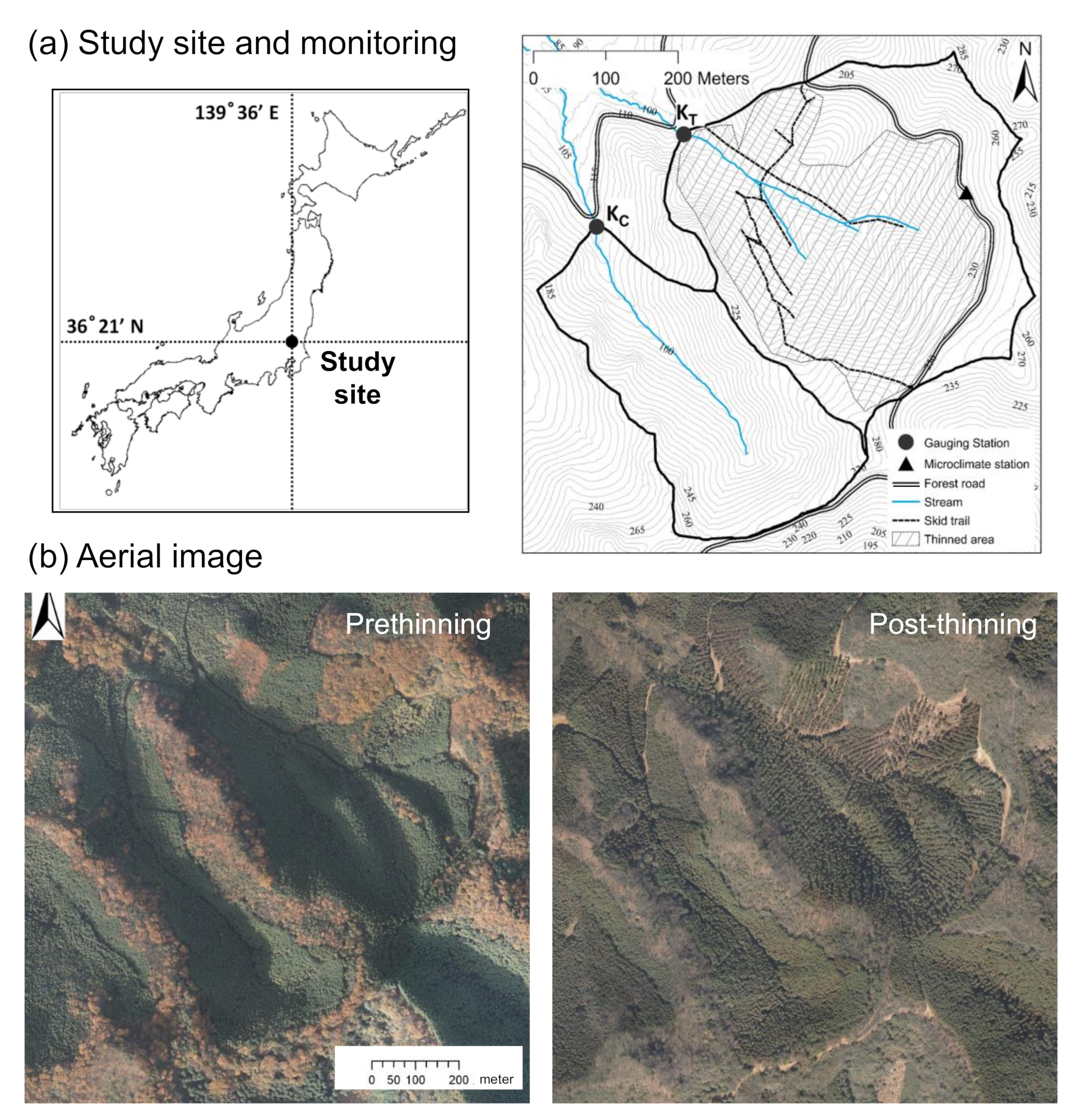
This study was conducted in two forested headwater catchments, KT (17.1 ha) and KC (8.9 ha), located in the area of Mt. Karasawa, Tochigi Prefecture, Japan (36°22′ N, 139°36′ E; Figure 1a). KT catchment was subjected to the thinning treatment, while KC catchment was maintained as a control (no thinning). The climate in this area is moist and temperate with 1234 ± 196 (mean ± standard deviation) mm mean annual precipitation and 14 ± 0.5 °C mean air temperature, based on an automated climate station located 3 km southwest of our study site (1994 to 2013 in Sano AMeDAS—Automatic Meteorological Data Acquisition System). High and intense precipitation occurs during the monsoon season (Baiu season) from May to July, and from August to October in association with typhoons. The study catchments range in elevation from 130 to 260 m a.s.l. [35]. Both catchments are underlain by sedimentary rock consisting of sandstone, chert, slate, mudstone, and shale. Stands of 20- to 50-year-old Japanese cedar (Cryptomeria japonica) and cypress (Chamaecyparis obtuse) dominate along the streams and up to the middle and upper parts of hillslopes. The ridgeline within the catchment is covered by mixture of broadleaf (e.g., Quercus serrata) and red pine (Pinus densiflora) forests. Dominant understory vegetation was evergreen shrubs (e.g., Cleyera japonica and Ardisia japonica) and Japanese aucuba (Aucuba japonica) before thinning. Stream channels have a mean gradient 6° (2° standard deviation), bankfull widths from 0.5 to 1.5 m and wetted widths from 0.2 to 1.0 m. Channel morphology includes pool–riffle and step–pool units [36] formed by boulders, cobbles and gravel.
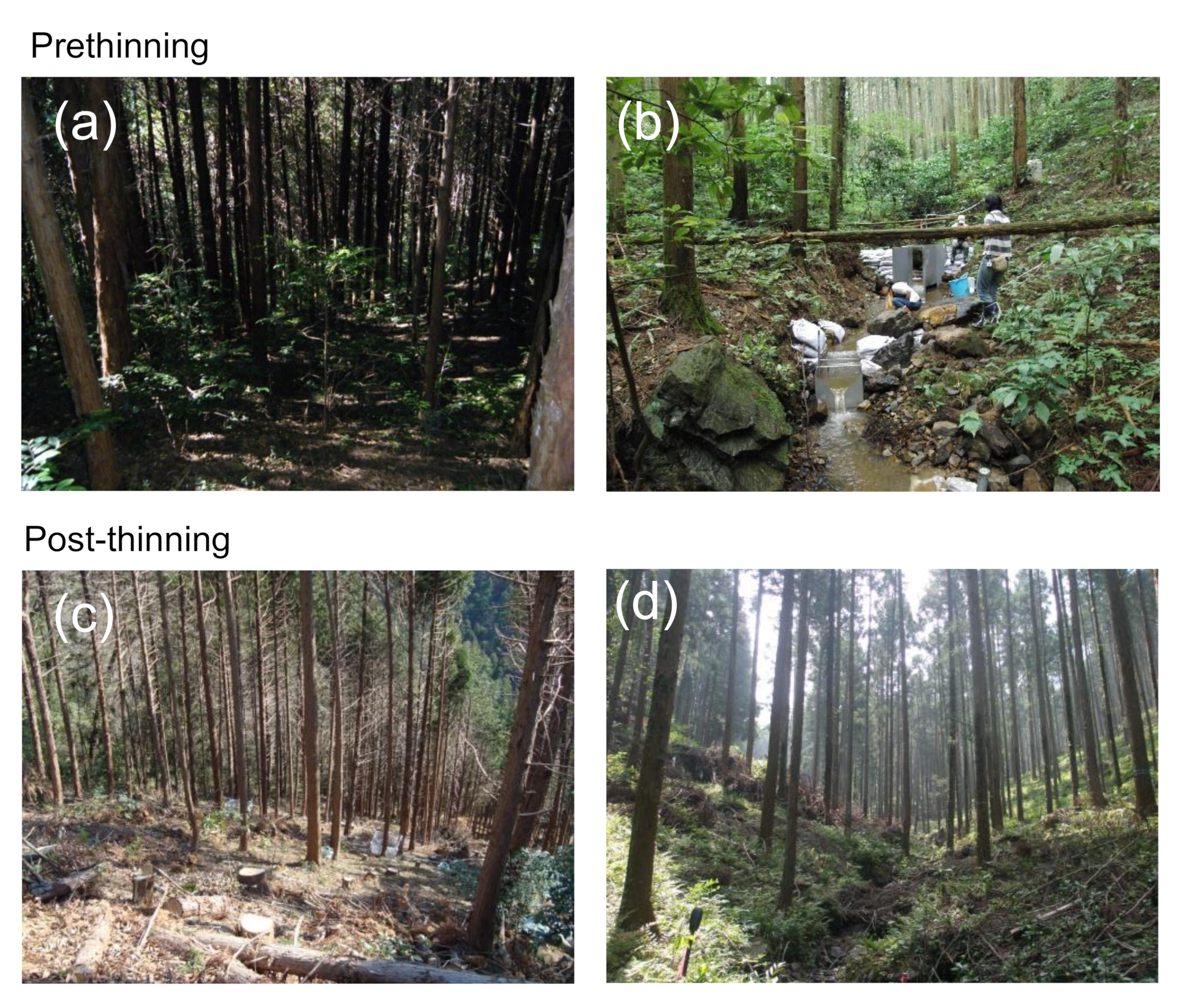
Thinning in KT catchment was conducted from July to December 2011 by removing two lines of plantation trees (Figure 1 and Figure 2). Stand density before thinning was 2198 stems ha−1, whereas stand density became 1099 stems ha−1 with a basal area of 26.2 m2 ha−1 after 50% strip-thinning [37]. Thinning extended from the upper hillslope to the riparian zones (Figure 2). All thinned trees were cut by chainsaw and cable-yarded to the road and/or skid trail. Logging roads were located at the middle of the hillslope in KT catchment and in the upper hillslope in KC catchment (Figure 1a). An old logging road and new skid trail were reactivated and/or installed at the bottom of the valley [35]. After thinning, fern species (Gleichenia japonica), evergreen shrubs (e.g., Cleyera japonica and Ardisia japonica), Japanese aucuba (Aucuba japonica), and herbs and grasses (Carex lanceolate and Trachelospermum asiaticum) dominated [38]. We defined the period from 30 June 2010 to 1 July 2011 as “prethinning” and from 1 January to 31 December 2012, as “post-thinning”. The period of forest operation with clearing understory vegetation and stand removal from July to December 2011 was considered as “during thinning operation”.
2.2. Monitoring
Discharge and stream temperature were monitored at the outlets of catchments KC and KT from April 2010. Discharge was measured using a combination of V-notch weirs for low to moderate flow and Parshall flumes for high flow (Figure 2b). In the KT catchment, we used a 90° V-notch weir and one-foot-wide Parshall flume, while a 60° V-notch weir and 5-inch-wide Parshall flume were installed at the KC catchment. Approximately 75% of flow data were estimated using the V-notch weirs and 25% using the Parshall flumes. TruTrack water level loggers (TruTrack WT-HR 1000, Trutrack Ltd, Christchurch, New Zealand) recorded stage height every 10 min at both the weirs and flumes. Discharge through the V-notch weirs was measured using the volumetric method to develop the stage–discharge relationships. Discharge through the Parshall flumes was calculated using a formula based on flume dimensions and observed water depth [39,40].
Continuous water temperature data at 10-min intervals were obtained by TruTrack loggers with ±0.3 °C precision. We also measured water temperature using Onset Tidbit water temperature data logger with ±0.2 °C precision (HOBO Water Temp v2, Onset Computer Corporation, Bourme, MA, USA) to confirm the accuracy of TruTrack logger. Water temperature measured by TruTrack loggers agreed with Tidbit data with a mean of the absolute values of the differences of 0.3 °C. We calculated daily maximum, minimum, and mean stream temperatures based on 10-min data.
Meteorological data were monitored using an automated weather station (HOBO U30-NRC Weather Station; Onset Computer Corporation, MA, USA) located at an open site at 250 m a.s.l. in the KT catchment (Figure 1). Precipitation (mm), solar radiation (W m−2), air temperature (°C), relative humidity (%), and wind speed (m s−1) were recorded every 5 min. All sensors were placed at 2 m height above the ground. Daytime mean solar radiation, air temperature, relative humidity, and wind speed were calculated based on data from 6:00 to 18:00 [37]. Daytime mean values were determined by averaging the 5 min data.
We obtained 339 days with complete data coverage in the pre-thinning period (27 days were missing data in both the KT and KC catchments) and 366 days in the post-thinning period from 1 January 2012 to 31 December 2012. Complete stream temperature records were available for analysis. However, equipment malfunction resulted in 39 days of missing data (4.3 % of total data) for the climate station in the post-thinning period. Discharge data were not available for 41 (4.5% of total data) and 33 days (3.6% of total data) in the KT and KC catchments, respectively.
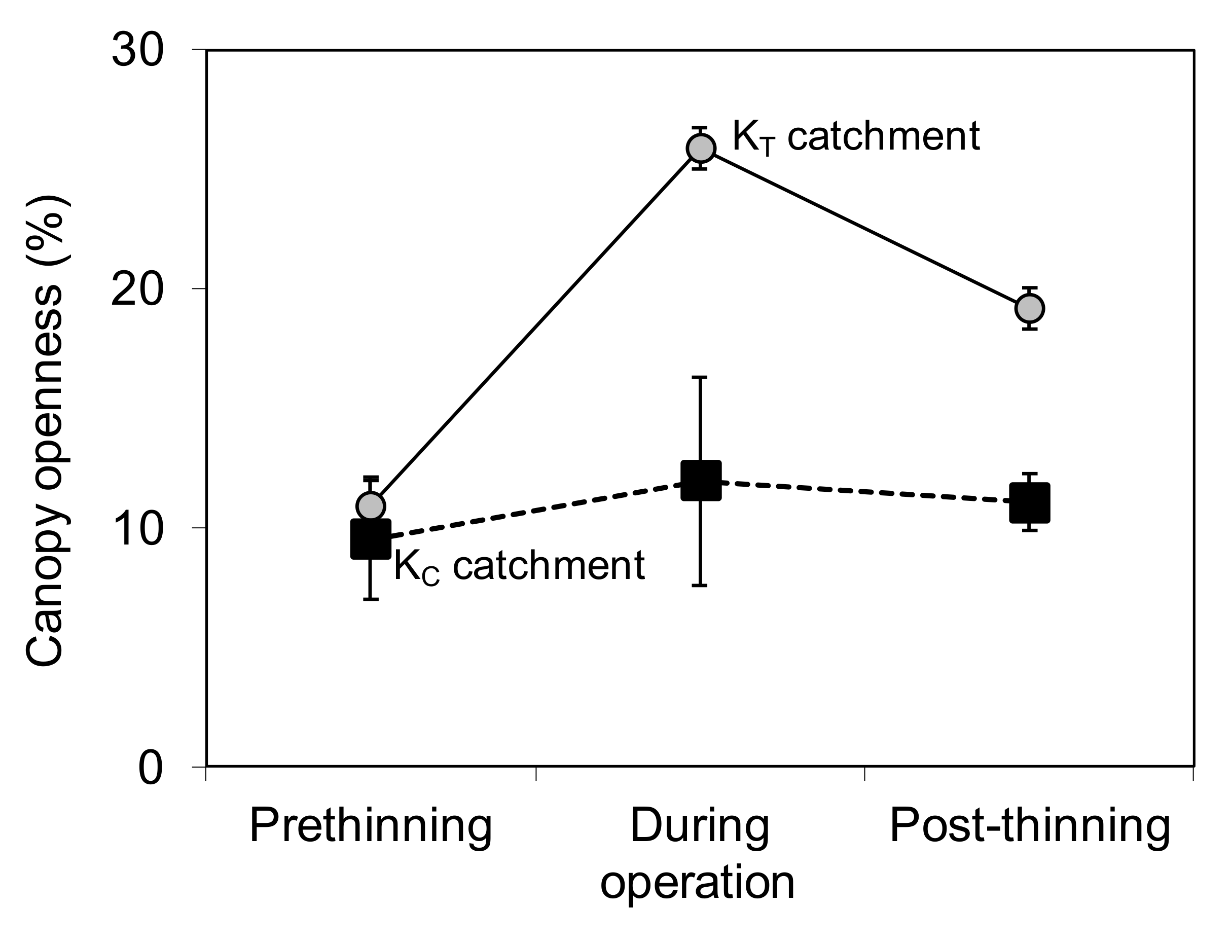
Canopy openness of the riparian forest was estimated by taking hemispherical photographs 50 cm above stream surface using a Nikon D40 camera equipped with a Sigma 8 mm fisheye lens. Prior to taking photographs, the camera was mounted on a tripod and was oriented to the north. Hemispherical images were taken at the KT and KC catchments on 16 December 2010, 16 December 2011, and 4 December 2012, for the pre-thinning, during operation, and post-thinning periods, respectively. Gap Light Analyzer software (GLA, version 2) was used to analyze hemispherical images [41].
2.3. Paired-Catchment Analysis of Stream Temperature Responses
Paired-catchment analysis was applied to detect the effects of thinning on daily mean, maximum, and minimum stream temperatures [25]. We fit the following model using daily stream temperature data for the pre-thinning period:
where is daily maximum, mean, or minimum temperatures at day t from the treated catchment KT, is the corresponding temperature variables at day t from the control catchment KC, β0, β1, β2, and β3 are coefficients to be determined by regression, j is the day of year (j = 1 corresponds to 1 January), and T = 365.25 is the number of days in a year [18]. The sine and cosine terms are included to account for seasonality in the residuals [42]. The error term, ɛt, was modeled as an autoregressive process of order “k”, expressed as:
where is the autocorrelation coefficient for the error terms at a lag of k days, is the error term k days before day t, and is a random disturbance. The value of k was determined based on finding the lowest value of Akaike’s information criterion (AIC) [43]. The pre-thinning calibration was performed using the arima() function in the R programming language [23].
We used the preharvest regression to predict what the stream temperatures in the treated catchment KT would have been for the post-thinning period had the treatment not occurred. The apparent changes in stream temperature resulting from the impacts of forest thinning were estimated as follows:
where Te is the treatment effect (°C) and is the observed stream temperature in the KT catchment on day t and is the predicted temperature on day t, based on the fitted regression model.
Prediction intervals were calculated using Monte Carlo simulation [6] using a confidence level of 95%. The uncertainty among the estimated parameters in the regression model for 1000 realizations was generated by function rmvnnorm() in the tmvnorm package in base R (R Development Core Team, 2019) to account for the variance–covariance structure of the parameter estimates.
Significance of the treatment effects was determined by applying the binomial distribution to the number of days on which the observed temperature fell outside the 95% prediction limits [44]. Under the null hypothesis of no treatment effect, one would expect to find kexp = n × p exceedances, where kexp is the expected number of exceedances, n is the number of days, and p is the probability of exceedance (0.05 for 95% prediction intervals). For large samples, the normal approximation to the binomial can be applied, and the probability associated with finding the observed number of exceedances, or more, is equal to the probability of sampling a random normal deviate greater than or equal to , where k is the observed number of exceedances.
2.4. Analysis of Hydrometeorological Controls
We examined factors controlling the variability of treatment effects using pairwise rank correlation analysis and multiple linear regression. Factors were selected using the underlying physical principle that stream temperature changes are positively related to surface energy exchange and inversely related to stream depth [9]. Explanatory variables therefore included the following meteorological controls on stream–surface energy fluxes: daytime mean solar radiation (W m−2), daily mean air temperature (°C), daily mean vapor pressure (, kPa) and daily mean wind speed (m s−1).
Daily mean air temperature is related to both incident longwave radiation and, in conjunction with wind speed, the sensible heat flux. Daytime mean air vapor pressure () is related to the latent heat exchange [45]. Air vapor pressure was calculated as:
where RH is the relative humidity (%) and is the saturation vapor pressure as a function of air pressure, calculated as:
Daily stream discharge (mm day−1) was also included in the analysis because it is related to stream depth [46]. In addition, higher stream discharge is typically associated with higher lateral inflow and advective heat transport [24], as well as higher in-stream velocities and thus reduced exposure time to energy inputs. We used the mean daily discharge instead of maximum or minimum because thermal responses of water tended to be associated with the mean condition of parameter in a given day. Analysis focused on the period from 1 April to 30 September, which was the period dominated by significant treatment effects.
We tested the association between treatment effects and hydrometeorological drivers using Spearman rank order correlation analysis. Rank correlation was used because it does not require assumptions about linearity of the relation or normality of data distributions.
Prior to conducting the regression analysis, all variables were standardized by subtracting the mean value and dividing by the standard deviation in order to assess the relative influence of each factor on treatment effects [47]. A stepwise regression using both forward and backward selection based on AIC was used to select the significant factors controlling the variability of treatment effects [48]. The final model with the lowest AIC score was selected and only explanatory variables significant at p-value < 0.05 were retained. Multicollinearity was examined using the variance inflation factor (VIF). We used VIF < 5 for indicating the absence of significant multicollinearity [49]. Data processing and analysis were carried out using the R programming language (R Development Core Team, 2019).
3. Results
3.1. Canopy Openness
Riparian canopy openness of the KT and KC catchments was similar in the pre-thinning period (Figure 3). During the strip-thinning operation, the mean canopy openness of the KT catchment became higher than that during the prethinning period with 25.9% ± 0.8%, while that of the KC catchment remained similar to that during prethinning at 11.1% ± 4.3% (Figure 3). One year after thinning, the mean canopy openness of the KT catchment was higher than that of the KC catchment.
3.2. Climatic Conditions
At the AMeDAS Sano climate station, mean air temperature during the monitoring periods was similar to the mean value of air temperature over the past 20 years. Daily air temperatures in the post-thinning period were slightly higher than those in the prethinning period (Table 1). Annual precipitation at AMeDAS Sano climate station in 2010, 2011, and 2012 were 1363, 1371, and 1218 mm, compared to the 20-year average of 1234 mm, that is, the prethinning and during-operation periods were wetter than the average year, while the post-thinning tended to be drier.
3.3. Hydrological Processes and Stream Temperature
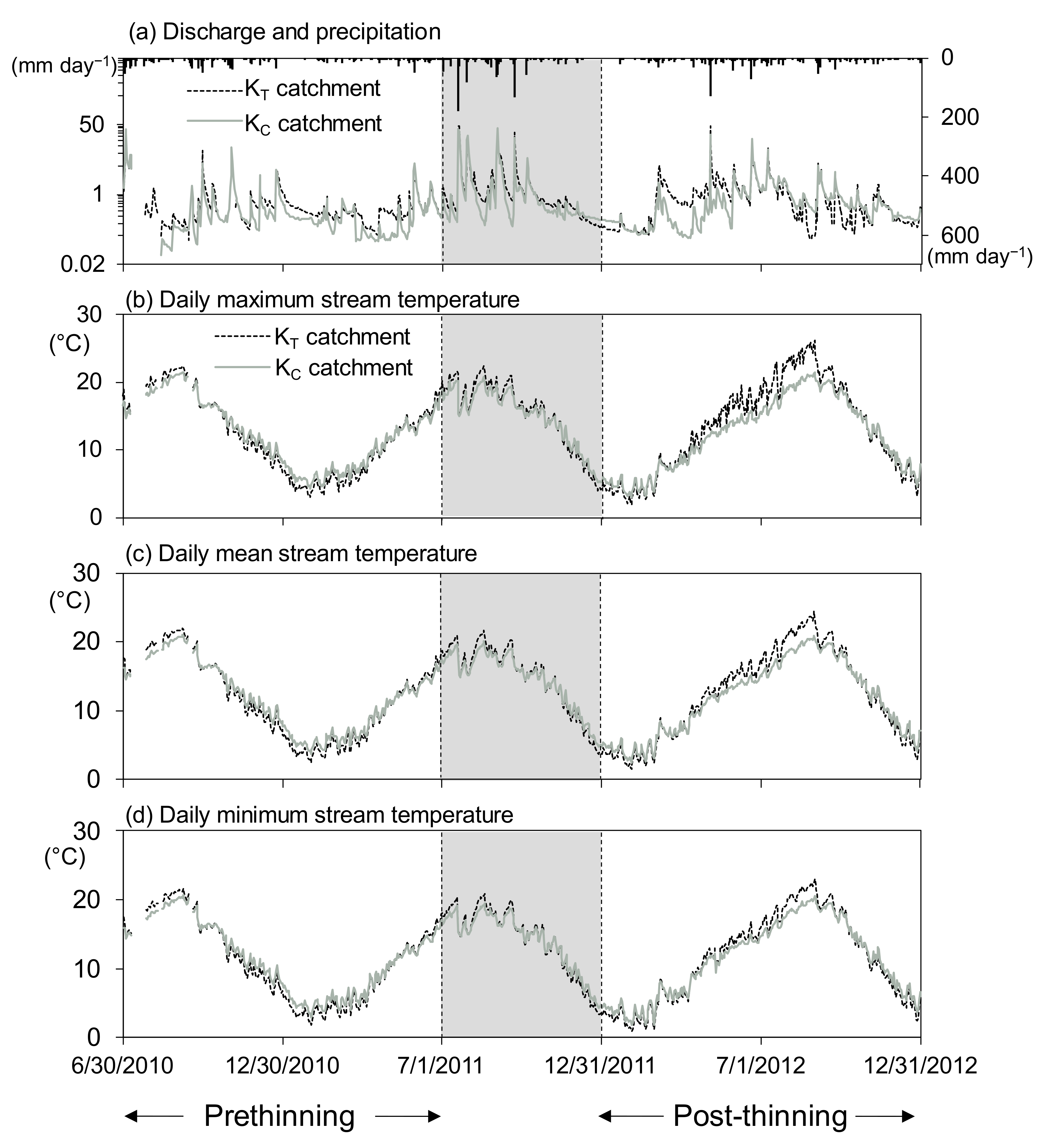
Runoff responded quickly to precipitation and was similar in both catchments (Figure 4). Total runoff from the KT catchment increased from 255 mm in the prethinning to 430 mm in the post-thinning period, while for the KC catchment, total runoff was 280 and 340 mm in pre- and post-thinning periods, respectively. The mean daily discharge of KC catchment was similar between the prethinning and post-thinning periods, while the mean daily discharge of KT catchment was 50% higher in the post-thinning (Table 1). Maximum prethinning discharge was 14.6 mm day−1 in the KT catchment and 38.2 mm day−1 in the KC catchment, which occurred on 2 July 2010 (28.4 mm day−1 total precipitation). The highest post-thinning discharge for KT (44.9 mm day−1) and KC (28.8 mm day−1) occurred on 3 May 2012 during a storm event with 126.8 mm day−1 rainfall. Minimum daily discharge with less than 1.0 mm day−1 occurred during winter periods when precipitation became low.
Daily stream temperature in the KT and KC catchments varied seasonally, with minimum temperatures occurring in January and February and maximum temperatures in August or September (Figure 4). Daily mean and maximum stream temperatures in the control catchment were generally similar in the pre- and post-thinning periods (Table 1). The daily mean stream temperature of the KT catchment was warmer in the post-thinning period, with the mean stream temperature ranging from 11.5 °C in the prethinning to 12.2 °C in the post-thinning period. The maximum temperature of KT catchment in the post-thinning period was higher than in the prethinning period. Daily minimum stream temperature of control and treated catchments were cooler than in the prethinning period. Observed minimum stream temperature in our study site remained above 0 °C even when air temperatures were lower than −1 °C.
3.4. Treatment Effects
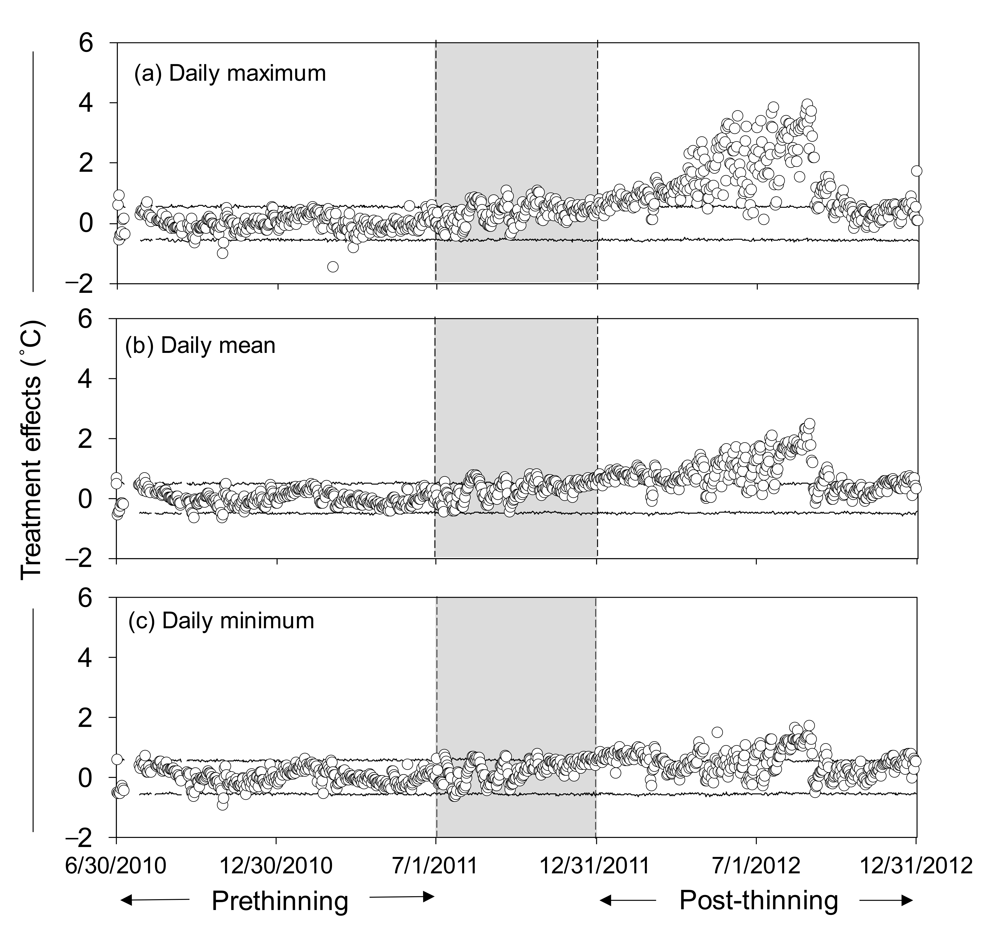
The prethinning regressions provided good fits to the data, with residual standard errors of 0.21°C, 0.14 °C, and 0.17 °C for daily maximum, mean, and minimum temperature, respectively. The prethinning calibration equations were all highly significant (p-values < 0.001) and regression coefficients were similar for daily maximum, mean, and minimum stream temperatures (Table 2). The autoregression coefficients for the residuals were significant up to five or six lags. Treatment effects were greatest for daily maximum temperature, lowest for daily minimum temperature, and intermediate for daily mean temperature (Table 3).
Between 1 January to 22 September 2012, treatment effects exceeded the 95% prediction interval for a total of 240 days for daily maximum temperature, 235 days for daily mean temperature, and 124 days for daily minimum temperature (Figure 5). Treatment effects were highly significant for all three stream temperature variables (Table 3). The maximum treatment effect for maximum daily stream temperature was 3.9 °C, which occurred on 27 August 2012, when maximum air temperature was 37.6 °C and daytime mean solar radiation was 412 Wm−2. Maximum treatment effects for daily mean and minimum stream temperature were 2.5 °C and 1.7 °C, respectively, and occurred on 31 August 2012, when maximum air temperature was 38.6 °C and daytime mean solar radiation was 411 Wm−2.
3.5. Analysis of Factors Controlling the Magnitude of Treatment Effects
Solar radiation, air temperature, and air vapor pressure were positively correlated with treatment effects for daily maximum and mean temperature (Table 4). Air temperature and air vapor pressure showed a significant positive correlation with treatment effects for daily minimum stream temperature. Stream discharge was strongly negatively correlated with treatment effects for daily maximum, mean, and minimum temperature (Table 4). When all explanatory variables were correlated among each other, air temperature was shown to be strongly positively correlated with air vapor pressure and solar radiation.
Multiple linear regression results identified solar radiation as the primary hydrometeorological control on the variability of treatment effects for daily maximum temperature (Table 5). Discharge had a significant negative relation with treatment effects, whereas air vapor pressure had significant positive effects. For daily mean stream temperature, stream discharge had the largest effect on the treatment effect in terms of the magnitude of the standardized coefficient, followed by air vapor pressure. For daily minimum stream temperature, stream discharge and air vapor pressure were significant influences on the treatment effect, with negative and positive coefficients, respectively.
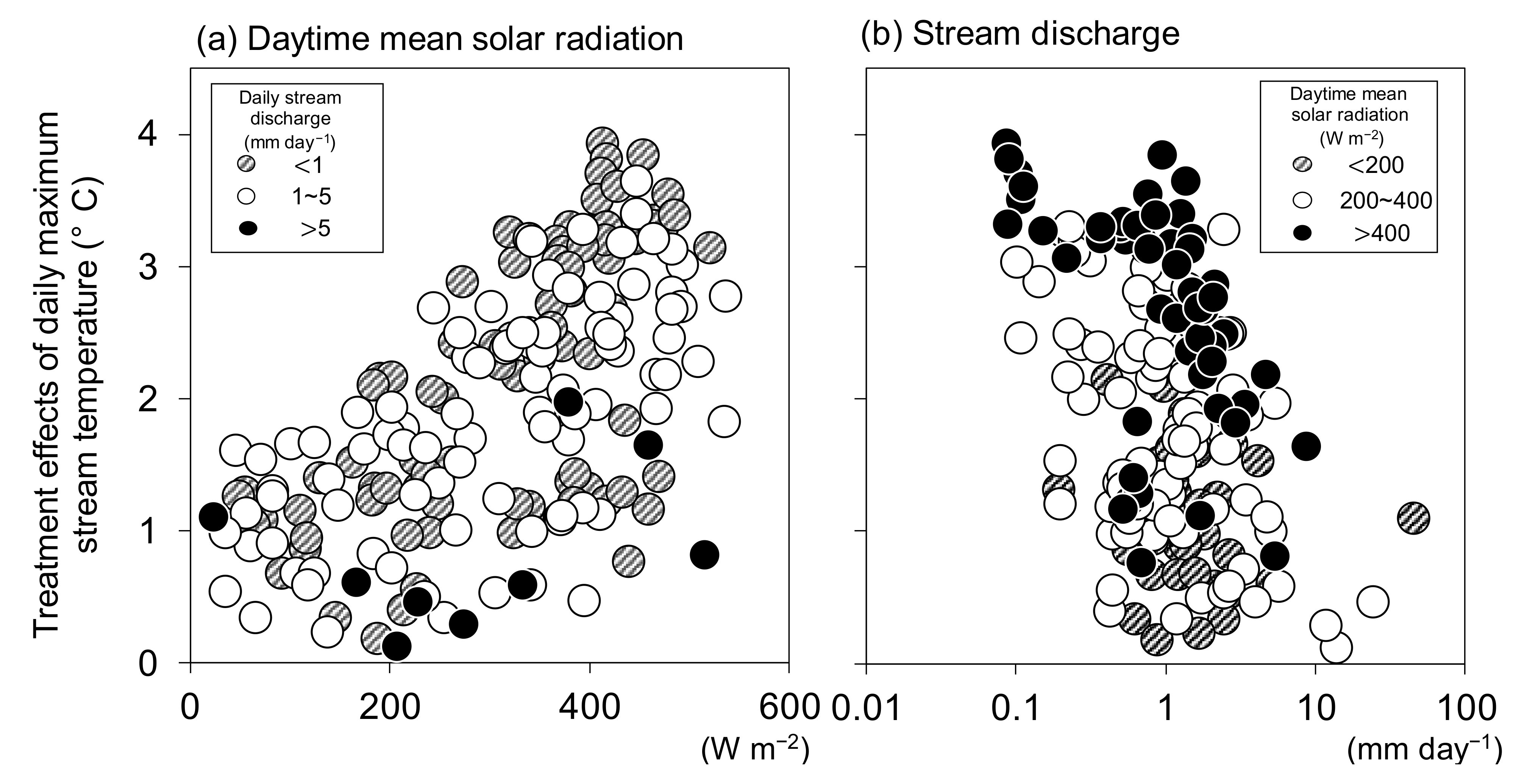
The highest treatment effects for daily maximum stream temperature occurred under conditions of both low flow (<1 mm day−1) and high solar radiation (>400 Wm−2), while moderate flows (from 1 to 5 mm day−1) tended to be associated with lower treatment effects even at high levels of solar radiation (Figure 6a). During the period of high air temperature (20 to 28 °C) and high solar radiation (400 to 530 Wm−2), moderate discharges from 1 to 5 mm day−1 reduced the mean of maximum treatment effects from 3.4 to 2.6 °C. Similarly, for a given intensity of solar radiation inputs, the treatment effect decreased with increases in stream discharge (Figure 6b).
Treatment effects exhibited distinctive variations during storm events and recession periods. Following a storm event from 5 July to 8 July 2012, solar radiation inputs for the next two days (9 July and 10 July 2012) were high: 458 and 476 Wm−2. However, treatment effects were only 1.6 to 2.2 °C because discharge was 5 to 10 times higher during the hydrograph recession period compared to low flow conditions (Figure 7b). Lower treatment effects during recession periods also occurred on 1 June and 2 June 2012 (Figure 7a). Treatment effects became 2.3 and 3.2 °C when discharge became similar to prestorm conditions on 15 July and 16 July 2012. When rainfall was too low to produce significant catchment runoff, treatment effects progressively increased after each storm event and reached the highest treatment effect on 27 August 2012 (Figure 7c).
4. Discussion
4.1. Effects of Riparian Forest Practices on Stream Temperature Responses
The paired-catchment methodology is a well-established research approach because it allows the separation of harvesting effects from climate effects. Therefore, this approach is more accurate in elucidating the impacts of forest harvesting on stream temperature than other approaches, such as spatial comparations or before–after studies with no control catchment. Based on a paired-catchment experimental approach, our study revealed that 50% strip-thinning significantly increased daily maximum, mean, and minimum stream temperature for the first year following harvesting. Canopy openness increased by 8% following thinning, producing increases in maximum daily stream temperature of up to 3.9 °C. Similar percentages of riparian canopy removal using different harvesting practices induced similar order of magnitude of changes in stream temperatures, although the patterns of canopy openness were different between strip-thinning and random thinning. For instance, based on a study in a 90-ha headwater catchment, Ontario, Canada, Kreutzweiser et al. [31] found that 50% random thinning in the riparian forest and resultant decreases in canopy openness from 86.3% to 83.9% elevated maximum temperature up to 4.4 °C. Guenther et al. [23] showed that 50% random thinning in a 10-ha headwater catchment decreased canopy closure by 14% and increased daily maximum stream temperature by up to 5.5 °C. Rex et al. [50] showed that partial harvesting with retention at least 10 trees per 100 m of channel length reduced stream shade by 50% and increased mean weekly maximum stream temperature by up to 6 °C.
Increases in stream temperature by strip-thinning had less impact on stream temperatures than clear-cut harvesting without riparian buffers, which has produced increases in daily maximum temperature of up to 11 °C [10,18,21,51]. However, thermal response to strip thinning was higher compared to harvesting with retention of riparian buffers. For instance, streams with 30-m-wide riparian buffers exhibited negligible elevation of maximum daily stream temperature after clear-cutting in headwater streams in British Columbia [52], while retention of 10-m-wide buffers kept warming to less than 2 °C [18]. Bladon et al. [53] showed that streams with 15-m-wide riparian buffers did not increase in daily mean stream temperature after forest harvesting in Needle Branch, Oregon Coast Range. Reiter et al. [54] showed that a headwater stream with a 15.2-m-wide buffer had no apparent stream temperature increases after forest thinning in the Trask River Watershed Study, Oregon Coast Range.
Contemporary forest harvesting practices typically cause less disturbance to riparian vegetation and soil compared to practices that were common until the 1980s, which often involved clear-cut harvesting with no riparian buffer and broadcast burning of slash. Because riparian vegetation and soil tend to be less disturbed by partial stand removal [55], availability of understory vegetation can help mitigate solar radiation inputs to streams under strip and random thinning or variable retention harvesting treatments [9,56]. Indeed, Gomi et al. [18] found that rapid thermal recovery among clear-cut channels was associated with recovery of understory vegetation.
4.2. Temporal Variability of Treatment Effects and Influence of Catchment Hydrology
Similar to previous studies in rain-dominated catchments, the treatment effects were low in winter and high in summer and were greater for daily maximum temperature compared to daily minimum temperature [18,23]. These patterns are consistent with solar radiation being a primary driver of postharvest warming. However, whereas the Pacific Northwest experiences seasonal low flows during summer and early autumn, the monsoon and typhoon seasons can produce moderate to high flows through most of the period of high stream temperature at these Japanese study sites.
Multiple linear regression analysis revealed that solar radiation had the largest impact on variations in treatment effects for daily maximum stream temperature. This finding is consistent with previous process-based studies identifying net radiation as the dominant component of total daytime energy exchange following forest harvesting [25,57]. Air temperature was positively correlated with treatment effects. This relation could reflect the direct influence of air temperature on energy inputs via sensible heat flux and incident longwave radiation. However, the relation could also reflect an indirect influence due to the significant correlation between air temperature and solar radiation. Air temperature was not included in the results of the multiple linear regression because it exhibited a collinearity with air vapor pressure (VIF = 17). The treatment effect had a positive relationship with the vapor pressure of the air, which is consistent with the influence of vapor pressure of air on energy inputs via the latent heat flux [58,59,60].
Stream discharge influenced the magnitudes of treatment effects for maximum, minimum, and mean daily stream temperatures. In particular, for maximum daily stream temperature, treatment effects under moderate discharges (from 1 to 5 mm day−1) tended to be lower than increases under lower discharges (<1 mm day−1). Similar to our findings, Janisch et al. [19] showed that the highly variable response of daily maximum stream temperature in clear-cut streams, from 0.2 to 3.6 °C, was not simply related to the effects of meteorological factors such as solar radiation inputs, but also depended on stream flow. Higher discharge may influence the treatment effect in three ways: (1) discharge is associated with water depth, which reduces stream thermal response to energy inputs; (2) increased discharge is associated with higher velocity and thus shorter residence time within channel reaches, which reduces the opportunity for heating; and (3) hillslope runoff is associated with advective heat transport, which influences the stream heat budget [61].
Forest harvesting can modify flow volume and hydrologic pathways from hillslopes, and thus may influence the magnitude of treatment effects. Based on detailed investigation in our study catchments, reduction of interception loss and transpiration after 50% strip-thinning increased the amount of water reaching the ground surface and soil matrix [62,63]. Therefore, combined effects of changes in runoff and solar radiation input need to be included for the analysis of effects of timber harvesting on stream temperature response.
Mixing of thermally stable and relatively cool deep soil water and/or groundwater during high flow events and hydrograph recession periods likely reduced the treatment effects in our study catchment [64,65]. Indeed, the influence of mixing water from various flow pathways on changes in stream temperature was confirmed by detailed monitoring in a headwater catchment in Ashiu, Japan [66]. Differences in the contribution of groundwater inflow to streams with different geology also need to be considered [5,20,67]. Nevertheless, dynamics of mixing subsurface and groundwater related to catchment internal hydrological processes is also an important factor for controlling the variability of treatment effects. Most previous process-based research on forestry and stream temperature focused on the effects of forest removal on stream–surface energy exchanges, especially solar radiation (e.g., [9,57]). However, the results of this study have highlighted the important role of catchment hydrology as a control on stream thermal responses to forestry.
5. Conclusions
The first objective of this study was to quantify the impacts of strip-thinning on stream temperature in a forested headwater catchment. Paired-catchment analysis was used to meet the first objective and demonstrated that removal of 50% of a forest stand by strip-thinning in a headwater catchment changed stream temperatures the first year following treatment. Maximum daily stream temperature increased up to 3.9 °C, which was similar to increases following 50% random thinning and variable retention harvesting in previous studies, but was greater than the effect of clear-cutting with retention of riparian buffers.
The findings obtained in this study support the second objective and demonstrated that the thermal response varied positively with solar radiation and negatively with stream discharge. Stream discharge response to rain events played a key role in moderating the heating associated with solar radiation inputs. Furthermore, our study site had frequent precipitation during summer associated with its Asian monsoon climate, in contrast to most previous studies, which were conducted at sites in North America and Europe that experience relatively dry summers.
These findings highlight the need for future studies focusing on sites with a broader range of climate, geology, and groundwater–surface water interactions to develop a fuller understanding of thermal responses to timber harvesting in headwater catchments.
Author Contributions
Conceptualization, resources, and supervision, T.G.; methodology, T.G., R.D.M., and D.Q.O.; validation, T.G. and R.D.M.; investigation, data curation, and writing—original draft preparation, D.Q.O.; writing—review and editing, all coauthors. All authors have read and agreed to the published version of the manuscript.
Funding
This study was supported by the Japan Science and Technology (JST), Core Research for Evolutional Science and Technology (CREST) projects entitled “Field and modeling studies on the effect of forest devastation on flooding and environmental issues” and “Development of Innovative Technologies for Increasing in Watershed Runoff and Improving River Environment by Management Practice of Devastated Forest Plantation”. Part of this study was supported by the Japan Society for Promotion of Science (Grant No. 16H02556).
Institutional Review Board Statement
Not applicable.
Informed Consent Statement
Not applicable.
Data Availability Statement
The data that support the findings of this study are available from the corresponding author, upon reasonable request.
Acknowledgments
We would like to thank the staffs of the Field Museum Karasawa, Tokyo University of Agriculture and Technology (TUAT). We also wish to thank all lab members of the Watershed Hydrology and Ecosystems Management Laboratory, TUAT for supporting field investigation and advice on this study.
Conflicts of Interest
The authors declare no conflict of interest.
References
- Becker, M.W.; Georgian, T.; Ambrose, H.; Siniscalchi, J.; Fredrick, K. Estimating flow and flux of ground water discharge using water temperature and velocity. J. Hydrol. 2004, 296, 221–233. [Google Scholar] [CrossRef]
- Westhoff, M.C.; Gooseff, M.N.; Bogaard, T.A.; Savenije, H.H.G. Quantifying hyporheic exchange at high spatial resolution using natural temperature variations along a first-order stream. Water Resour. Res. 2011, 47, W10508. [Google Scholar] [CrossRef] [Green Version]
- Gomi, T.; Sidle, R.C.; Richardson, J.S. Understanding processes and downstream linkages of headwater systems. Bioscience 2002, 52, 905–916. [Google Scholar] [CrossRef] [Green Version]
- Webb, B.W.; Clack, P.D.; Walling, D.E. Water-air temperature relationships in a Devon river system and the role of flow. Hydrol. Process. 2003, 17, 3069–3084. [Google Scholar] [CrossRef]
- Tague, C.; Farrell, M.; Grant, G.; Lewis, S.; Rey, S. Hydrogeologic controls on summer stream temperatures in the McKenzie River basin, Oregon. Hydrol. Process. 2007, 21, 3288–3300. [Google Scholar] [CrossRef]
- Leach, J.A.; Moore, R.D.; Hinch, S.G.; Gomi, T. Estimation of forest harvesting-induced stream temperature changes and bioenergetic consequences for cutthroat trout in a coastal stream in British Columbia, Canada. Aquat. Sci. 2012, 74, 427–441. [Google Scholar] [CrossRef]
- Richardson, J.S. Biological Diversity in Headwater Streams. Water 2019, 11, 366. [Google Scholar] [CrossRef] [Green Version]
- Webb, B.W.; Hannah, D.M.; Moore, R.D.; Brown, L.E.; Nobilis, F. Recent advances in stream and river temperature research. Hydrol. Process. 2008, 22, 902–918. [Google Scholar] [CrossRef]
- Moore, R.D.; Spittlehouse, D.L.; Story, A. Riparian microclimate and stream temperature response to forest harvesting: A review. J. Am. Water Resour. Assoc. 2005, 41, 813–834. [Google Scholar] [CrossRef]
- Harris, D.D. Hydrologic Changes after Logging in two Small Oregon Coastal Watersheds; Department of the Interior, Geological Survey: Burlington, MA, USA, 1977; Volume 2037. [Google Scholar] [CrossRef]
- Webb, B.W.; Crisp, D.T. Afforestation and stream temperature in a temperate maritime environment. Hydrol. Process. 2006, 20, 51–66. [Google Scholar] [CrossRef]
- Carlson, K.M.; Curran, L.M.; Ponette-Gonzalez, A.G.; Ratnasari, D.; Lisnawati, N.; Purwanto, Y.; Brauman, K.A.; Raymond, P.A. Influence of watershed-climate interactions on stream temperature, sediment yield, and metabolism along a land use intensity gradient in Indonesian Borneo. J. Geophys. Res. Biogeo. 2014, 119, 1110–1128. [Google Scholar] [CrossRef]
- Raulerson, S.; Jackson, C.R.; Melear, N.D.; Younger, S.E.; Dudley, M.; Elliott, K.J. Do southern Appalachian Mountain summer stream temperatures respond to removal of understory rhododendron thickets? Hydrol. Process. 2020, 34, 3045–3060. [Google Scholar] [CrossRef]
- Wilkerson, E.; Hagan, J.M.; Siegel, D.; Whitman, A.A. The effectiveness of different buffer widths for protecting headwater stream temperature in Maine. Forest Sci. 2006, 52, 221–231. [Google Scholar]
- Groom, J.D.; Dent, L.; Madsen, L.J.; Fleuret, J. Response of western Oregon (USA) stream temperatures to contemporary forest management. Forest Ecol. Manag. 2011, 262, 1618–1629. [Google Scholar] [CrossRef]
- Bowler, D.E.; Mant, R.; Orr, H.; Hannah, D.M.; Pullin, A.S. What are the effects of wooded riparian zones on stream temperature? Environ. Evid. 2012, 1, 1–9. [Google Scholar] [CrossRef] [Green Version]
- Groom, J.D.; Johnson, S.L.; Seeds, J.D.; Ice, G.G. Evaluating Links Between Forest Harvest and Stream Temperature Threshold Exceedances: The Value of Spatial and Temporal Data. J. Am. Water Resour. Assoc. 2017, 53, 761–773. [Google Scholar] [CrossRef]
- Gomi, T.; Moore, R.D.; Dhakal, A.S. Headwater stream temperature response to clear-cut harvesting with different riparian treatments, coastal British Columbia, Canada. Water Resour. Res. 2006, 42, W08437. [Google Scholar] [CrossRef]
- Janisch, J.E.; Wondzell, S.M.; Ehinger, W.J. Headwater stream temperature: Interpreting response after logging, with and without riparian buffers, Washington, USA. Forest Ecol. Manag. 2012, 270, 302–313. [Google Scholar] [CrossRef]
- Bladon, K.D.; Segura, C.; Cook, N.A.; Bywater-Reyes, S.; Reiter, M. A multicatchment analysis of headwater and downstream temperature effects from contemporary forest harvesting. Hydrol. Process. 2018, 32, 293–304. [Google Scholar] [CrossRef]
- Johnson, S.L.; Jones, J.A. Stream temperature responses to forest harvest and debris flows in western Cascades, Oregon. Can. J. Fish. Aquat. Sci. 2000, 57, 30–39. [Google Scholar] [CrossRef]
- Quinn, J.M.; Wright-Stow, A.E. Stream size influences stream temperature impacts and recovery rates after clearfell logging. Forest Ecol. Manag. 2008, 256, 2101–2109. [Google Scholar] [CrossRef]
- Guenther, S.M.; Gomi, T.; Moore, R.D. Stream and bed temperature variability in a coastal headwater catchment: Influences of surface-subsurface interactions and partial-retention forest harvesting. Hydrol. Process. 2014, 28, 1238–1249. [Google Scholar] [CrossRef]
- Leach, J.A.; Moore, D. Insights on stream temperature processes through development of a coupled hydrologic and stream temperature model for forested coastal headwater catchments. Hydrol. Process. 2017, 31, 3160–3177. [Google Scholar] [CrossRef]
- Moore, R.D.; Sutherland, P.; Gomi, T.; Dhakal, A. Thermal regime of a headwater stream within a clear-cut, coastal British Columbia, Canada. Hydrol. Process. 2005, 19, 2591–2608. [Google Scholar] [CrossRef]
- Hockey, J.; Owens, I.; Tapper, N. Empirical and theoretical models to isolate the effect of discharge on summer water temperatures in the Hurunui River. J. Hydrol. 1982, 21, 1–12. [Google Scholar]
- Du, X.Z.; Goss, G.; Faramarzi, M. Impacts of Hydrological Processes on Stream Temperature in a Cold Region Watershed Based on the SWAT Equilibrium Temperature Model. Water 2020, 12, 1112. [Google Scholar] [CrossRef] [Green Version]
- Vano, J.A.; Nijssen, B.; Lettenmaier, D.P. Seasonal hydrologic responses to climate change in the Pacific Northwest. Water Resour. Res. 2015, 51, 1959–1976. [Google Scholar] [CrossRef]
- Swanson, F.J.; Franklin, J.F. New Forestry Principles from Ecosystem Analysis of Pacific-Northwest Forests. Ecol. Appl. 1992, 2, 262–274. [Google Scholar] [CrossRef]
- Mitchell, S.J.; Beese, W.J. The retention system: Reconciling variable retention with the principles of silvicultural systems. For. Chron. 2002, 78, 397–403. [Google Scholar] [CrossRef]
- Kreutzweiser, D.P.; Capell, S.S.; Holmes, S.B. Stream temperature responses to partial-harvest logging in riparian buffers of boreal mixedwood forest watersheds. Can. J. Forest Res. 2009, 39, 497–506. [Google Scholar] [CrossRef]
- Maleque, M.A.; Ishii, H.T.; Maeto, K.; Taniguchi, S. Line thinning fosters the abundance and diversity of understory Hymenoptera (Insecta) in Japanese cedar (Cryptomeria japonica D. Don) plantations. J. Forest Res. 2007, 12, 14–23. [Google Scholar] [CrossRef]
- Ishii, H.T.; Maleque, M.A.; Shingo, T.G. Line thinning promotes stand growth and understory diversity in Japanese cedar (Cryptomeria japonica D. Don) plantations. J. Forest Res. 2008, 13, 73–78. [Google Scholar] [CrossRef]
- Kerr, G.; Haufe, J. Thinning Practice: A Silvicultural Guide. Forestry Commission. 2011. Available online: https://www.forestresearch.gov.uk/documents/4992/Silviculture_Thinning_Guide_v1_Jan2011.pdf (accessed on 5 April 2021).
- Nam, S.; Hiraoka, M.; Gomi, T.; Dung, B.X.; Onda, Y.; Kato, H. Suspended-sediment responses after strip thinning in headwater catchments. Landsc. Ecol. Eng. 2016, 12, 197–208. [Google Scholar] [CrossRef]
- Montgomery, D.R.; Buffington, J.M. Channel-reach morphology in mountain drainage basins. Geol. Soc. Am. Bull. 1997, 109, 596–611. [Google Scholar] [CrossRef]
- Sun, X.C.; Onda, Y.; Kato, H.; Otsuki, K.; Gomi, T. Partitioning of the total evapotranspiration in a Japanese cypress plantation during the growing season. Ecohydrology 2014, 7, 1042–1053. [Google Scholar] [CrossRef]
- Lopez-Vicente, M.; Sun, X.C.; Onda, Y.; Kato, H.; Gomi, T.; Hiraoka, M. Effect of tree thinning and skidding trails on hydrological connectivity in two Japanese forest catchments. Geomorphology 2017, 292, 104–114. [Google Scholar] [CrossRef] [Green Version]
- Herschy, R.W. Streamflow Measurement; Elsevier Applied Science: New York, NY, USA, 1985. [Google Scholar]
- Dung, B.X.; Gomi, T.; Miyata, S.; Sidle, R.C.; Kosugi, K.; Onda, Y. Runoff responses to forest thinning at plot and catchment scales in a headwater catchment draining Japanese cypress forest. J. Hydrol. 2012, 444, 51–62. [Google Scholar] [CrossRef]
- Frazer, G.W.; Canham, C.D.; Lertzman, K.P. Gap Light Analyzer (GLA), Version 2.0: Imaging Software to Extract Canopy Structure and Gap Light Transmission Indices from True-Colour Fisheye Photographs, Users Manual and Program Documentation; Simon Fraser University: Burnaby, BC, Canada; The Institute of Ecosystem Studies: Millbrook, NY, USA, 1999; Volume 36. [Google Scholar]
- Watson, F.; Vertessy, R.; McMahon, T.; Rhodes, B.; Watson, I. Improved methods to assess water yield changes from paired-catchment studies: Application to the Maroondah catchments. Forest Ecol. Manag. 2001, 143, 189–204. [Google Scholar] [CrossRef]
- Akaike, H. A new look at the statistical model identification. IEEE Trans. Automat. Control 1974, 19, 716–723. [Google Scholar] [CrossRef]
- Som, N.A.; Zegre, N.P.; Ganio, L.M.; Skaugset, A.E. Corrected prediction intervals for change detection in paired watershed studies. Hydrolog. Sci. J. 2012, 57, 134–143. [Google Scholar] [CrossRef] [Green Version]
- Webb, B.W.; Zhang, Y. Spatial and seasonal variability in the components of the river heat budget. Hydrol. Process. 1997, 11, 79–101. [Google Scholar] [CrossRef]
- MacDonald, R.J.; Boon, S.; Byrne, J.M.; Silins, U. A comparison of surface and subsurface controls on summer temperature in a headwater stream. Hydrol. Process. 2014, 28, 2338–2347. [Google Scholar] [CrossRef]
- Greenacre, M.; Primicerio, R. Multivariate Analysis of Ecological Data; Fundacion BBVA: Bilbao, Spain, 2014; Available online: https://www.fbbva.es/wp-content/uploads/2017/05/dat/DE_2013_multivariate.pdf (accessed on 5 April 2021).
- Yamashita, T.; Yamashita, K.; Kamimura, R. A stepwise AIC method for variable selection in linear regression. Commun. Stat. Theor. M 2007, 36, 2395–2403. [Google Scholar] [CrossRef]
- Neter, J.; Kutner, M.H.; Nachtsheim, C.J.; Wasserman, W. Applied Linear Statistical Models; McGraw-Hill/Irwin, WCB McGraw-Hill: New York, NY, USA, 1996; Volume 4. [Google Scholar]
- Rex, J.F.; Maloney, D.A.; Krauskopf, P.N.; Beaudry, P.G.; Beaudry, L.J. Variable-retention riparian harvesting effects on riparian air and water temperature of sub-boreal headwater streams in British Columbia. Forest Ecol. Manag. 2012, 269, 259–270. [Google Scholar] [CrossRef]
- Brown, G.W.; Krygier, J.T. Effects of clear-cutting on stream temperature. Water Resour. Res. 1970, 6, 1133–1139. [Google Scholar] [CrossRef]
- Kiffney, P.M.; Richardson, J.S.; Bull, J.P. Responses of periphyton and insects to experimental manipulation of riparian buffer width along forest streams. J. Appl. Ecol. 2003, 40, 1060–1076. [Google Scholar] [CrossRef]
- Bladon, K.D.; Cook, N.A.; Light, J.T.; Segura, C. A catchment-scale assessment of stream temperature response to contemporary forest harvesting in the Oregon Coast Range. Forest Ecol. Manag. 2016, 379, 153–164. [Google Scholar] [CrossRef]
- Reiter, M.; Johnson, S.L.; Homyack, J.; Jones, J.E.; James, P.L. Summer stream temperature changes following forest harvest in the headwaters of the Trask River watershed, Oregon Coast Range. Ecohydrology 2020, 13, e2178. [Google Scholar] [CrossRef]
- Bescond, H.; Fenton, N.J.; Bergeron, Y. Partial harvests in the boreal forest: Response of the understory vegetation five years after harvest. Forest Chron. 2011, 87, 86–98. [Google Scholar] [CrossRef] [Green Version]
- Gravelle, J.A.; Link, T.E. Influence of timber harvesting on headwater peak stream temperatures in a northern Idaho watershed. Forest Sci. 2007, 53, 189–205. [Google Scholar]
- Brown, G.W. Predicting temperatures of small streams. Water Resour. Res. 1969, 5, 68–75. [Google Scholar] [CrossRef] [Green Version]
- Hannah, D.M.; Malcolm, I.A.; Soulsby, C.; Youngson, A.F. Heat exchanges and temperatures within a salmon spawning stream in the cairngorms, Scotland: Seasonal and sub-seasonal dynamics. River Res. Appl. 2004, 20, 635–652. [Google Scholar] [CrossRef]
- Leach, J.A.; Moore, R.D. Above-stream microclimate and stream surface energy exchanges in a wildfire-disturbed riparian zone. Hydrol. Process. 2010, 24, 2369–2381. [Google Scholar] [CrossRef]
- Szeitz, A.J.; Moore, R.D. Predicting evaporation from mountain streams. Hydrol. Process. 2020, 34, 4262–4279. [Google Scholar] [CrossRef]
- Leach, J.A.; Moore, R.D. Winter stream temperature in the rain-on-snow zone of the Pacific Northwest: Influences of hillslope runoff and transient snow cover. Hydrol. Earth Syst. Sci. 2014, 18, 819–838. [Google Scholar] [CrossRef] [Green Version]
- Sun, X.C.; Onda, Y.; Chiara, S.; Kato, H.; Gomi, T. The effect of strip thinning on spatial and temporal variability of throughfall in a Japanese cypress plantation. Hydrol. Process. 2015, 29, 5058–5070. [Google Scholar] [CrossRef]
- Sun, X.C.; Onda, Y.; Otsuki, K.; Kato, H.; Gomi, T.; Liu, X.Y. Change in evapotranspiration partitioning after thinning in a Japanese cypress plantation. Trees Struct. Funct. 2017, 31, 1411–1421. [Google Scholar] [CrossRef]
- Sidle, R.C.; Tsuboyama, Y.; Noguchi, S.; Hosoda, I.; Fujieda, M.; Shimizu, T. Stormflow generation in steep forested headwaters: A linked hydrogeomorphic paradigm. Hydrol. Process. 2000, 14, 369–385. [Google Scholar] [CrossRef]
- Gomi, T.; Asano, Y.; Uchida, T.; Onda, Y.; Sidle, R.C.; Miyata, S.; Kosugi, K.; Mizugaki, S.; Fukuyama, T.; Fukushima, T. Evaluation of storm runoff pathways in steep nested catchments draining a Japanese cypress forest in central Japan: A geochemical approach. Hydrol. Process. 2010, 24, 550–566. [Google Scholar] [CrossRef]
- Uchida, T.; Kosugi, K.; Mizuyama, T. Effects of pipe flow and bedrock groundwater on runoff generation in a steep headwater catchment in Ashiu, central Japan. Water Resour. Res. 2002, 38, 1119. [Google Scholar] [CrossRef]
- Onda, Y.; Tsujimura, M.; Fujihara, J.I.; Ito, J. Runoff generation mechanisms in high-relief mountainous watersheds with different underlying geology. J. Hydrol. 2006, 331, 659–673. [Google Scholar] [CrossRef]
Figure 1.
(a) Locations of study site and monitoring stations; (b) aerial images of study catchments before and after thinning.
Figure 1.
(a) Locations of study site and monitoring stations; (b) aerial images of study catchments before and after thinning.

Figure 2.
Overview of (a) hillslope and (c) riparian conditions before thinning and (c) hillslope and (d) riparian condition after thinning. In photo (b), one can also see the monitoring station of the KT catchment with combination of Parshall flume and box type V-notch weir.
Figure 2.
Overview of (a) hillslope and (c) riparian conditions before thinning and (c) hillslope and (d) riparian condition after thinning. In photo (b), one can also see the monitoring station of the KT catchment with combination of Parshall flume and box type V-notch weir.

Figure 3.
The changes in canopy openness (%) in the treated (KT) and control (KC) catchments during our monitoring period. Prethinning, during-operation, and post-thinning canopy openness was measured on 16 December 2010, 16 December 2011, and 4 December 2012, respectively.
Figure 3.
The changes in canopy openness (%) in the treated (KT) and control (KC) catchments during our monitoring period. Prethinning, during-operation, and post-thinning canopy openness was measured on 16 December 2010, 16 December 2011, and 4 December 2012, respectively.

Figure 4.
(a) Daily stream discharge and total daily precipitation, (b) daily maximum stream temperatures, (c) daily mean stream temperatures, and (d) daily minimum stream temperatures at the KT and KC catchments. Shaded area indicates during thinning operation period.
Figure 4.
(a) Daily stream discharge and total daily precipitation, (b) daily maximum stream temperatures, (c) daily mean stream temperatures, and (d) daily minimum stream temperatures at the KT and KC catchments. Shaded area indicates during thinning operation period.

Figure 5.
Time series of treatment effects for (a) daily maximum stream temperature, (b) daily mean stream temperature, and (c) daily minimum stream temperature at the KT catchment. The black horizontal lines indicated 95% prediction intervals for treatment effects. Shaded area indicates during thinning operation period.

Figure 6.
(a) Relationship between daytime mean solar radiation and treatment effects of daily maximum stream temperature by the classification of discharge classes. (b) Relationship between stream discharge and treatment effects of daily maximum stream temperature by the classification of solar radiation classes. Data from April to September 2012 were used for these plots.

Figure 7.
Changes in precipitation, runoff, climate condition, and treatment effect in selected periods of May (a), July (b), and August (c) in the post-thinning period. (a) Period 1 from 23 May to 6 June 2012 had less increase in discharge, (b) period 2 from 2 July to 16 July 2012, discharge increased significantly after storm events, and (c) period 3 from 13 August to 27 August 2012 had low rainfall and discharge.


Table 1.
Summary of air temperature, stream discharge, and stream temperatures.
| Prethinning | During Thinning Operation | Post-Thinning | |
|---|---|---|---|
| Total rainfall (mm) | 1230 | 1040 | 1295 |
| Air temperature (°C) | |||
| Max | 37.9 | 37.9 | 38.6 |
| Mean | 14.2 | 18.9 | 15.1 |
| SD | 8.7 | 6.9 | 8.3 |
| Min | −4.6 | 0.0 | −5.7 |
| Discharge (mm day−1) | |||
| KT catchment | |||
| Max | 14.6 | 44.3 | 44.9 |
| Mean | 0.8 | 2.6 | 1.2 |
| SD | 1.6 | 6.3 | 2.9 |
| Min | 0.1 | 0.2 | 0.1 |
| KC catchment | |||
| Max | 38.2 | 39.0 | 28.8 |
| Mean | 0.8 | 2.2 | 0.9 |
| SD | 3.0 | 5.8 | 2.1 |
| Min | 0.1 | 0.2 | 0.1 |
| Stream temperature (°C) | |||
| KT catchment | |||
| Max | 22.3 | 22.4 | 26.2 |
| Mean | 11.5 | 14.8 | 12.2 |
| SD | 5.6 | 4.8 | 6.4 |
| Min | 1.8 | 3.1 | 0.9 |
| KC catchment | |||
| Max | 21.5 | 20.8 | 21.5 |
| Mean | 11.8 | 14.5 | 11.7 |
| SD | 4.8 | 4.1 | 5.3 |
| Min | 2.8 | 4.2 | 1.8 |
Table 2.
Results of ARIMAX analysis for prethinning calibration.
| Stream Temperature Variables | b Estimates | k | |||||||||
|---|---|---|---|---|---|---|---|---|---|---|---|
| Intercept | KC | Sine | Cosine | ||||||||
| (s.e.) | (s.e.) | (s.e.) | (s.e.) | (s.e.) | (s.e.) | (s.e.) | (s.e.) | (s.e.) | (s.e.) | ||
| Daily maximum | −1.51 | 1.11 | 0.04 | −0.58 | 6 | 0.522 | 0.03 | 0.05 | −0.06 | 0.08 | 0.13 |
| (0.27) | (0.02) | (0.12) | (0.11) | (0.06) | (0.07) | (0.06) | (0.06) | (0.06) | (0.06) | ||
| Daily mean | −1.94 | 1.14 | 0.33 | −0.42 | 5 | 0.8 | −0.13 | 0.07 | −0.05 | 0.15 | - |
| (0.2) | (0.02) | (0.15) | (0.01) | (0.06) | (0.07) | (0.07) | (0.07) | (0.06) | |||
| Daily minimum | −1.64 | 1.12 | 0.27 | −0.51 | 6 | 0.64 | 0.06 | −0.03 | 0.04 | 0.03 | 0.1 |
| (0.22) | (0.02) | (0.12) | (0.12) | (0.06) | (0.07) | (0.07) | (0.07) | (0.07) | (0.06) | ||
k is order of the residual autocorrelation, is the estimated lag i autocorrelation coefficient of residuals. The regression coefficients b are estimated for the parameters β with standard errors (s.e.) shown in brackets.
Table 3.
Summary of residuals of prethinning regression, treatment effects, and the significance of treatment effects.
Table 3.
Summary of residuals of prethinning regression, treatment effects, and the significance of treatment effects.
| Stream Temperature Variables | Residuals (°C) | Treatment Effects (Te) (°C) | Significance of Te | ||||||||
|---|---|---|---|---|---|---|---|---|---|---|---|
| Prethinning | Post-Thinning | k | z-Score | p-Value | |||||||
| (n = 339) | (n = 366) | ||||||||||
| Max | Mean | SD | Min | Max | Mean | SD | Min | ||||
| Daily maximum | 0.9 | 0.0 | 0.2 | −1.5 | 3.9 | 1.3 | 1.0 | −0.2 | 240 | 85 | <0.001 |
| Daily mean | 0.7 | 0.0 | 0.2 | −0.7 | 2.5 | 0.8 | 0.5 | −0.2 | 235 | 83 | <0.001 |
| Daily minimum | 0.7 | 0.0 | 0.3 | −0.9 | 1.7 | 0.5 | 0.4 | −0.5 | 124 | 40 | <0.001 |
k is the observed number of exceedences, n is the sample size.
Table 4.
Spearman rank correlation coefficients between treatment effects and hydrometeorological variables.
Table 4.
Spearman rank correlation coefficients between treatment effects and hydrometeorological variables.
| Solar Radiation | Air Temperature | Air Vapor Pressure | Wind Speed | Discharge | |
|---|---|---|---|---|---|
| Daily maximum | 0.61 ** | 0.47 ** | 0.37 *** | 0.07 | −0.31 ** |
| Daily mean | 0.35 ** | 0.52 ** | 0.48 *** | 0.09 | −0.45 ** |
| Daily minimum | 0.03 | 0.44 ** | 0.47 *** | 0.21 * | −0.55 ** |
| Solar radiation | 1 | 0.4 ** | 0.04 | 0.31 ** | −0.03 |
| Air temperature | 1 | 0.9 *** | 0.11 | −0.25 * | |
| Air vapor pressure | 1 | 0.01 | −0.21 * | ||
| Wind speed | 1 | −0.21 * | |||
| Discharge | 1 |
Significance level: * p-value < 0.05, ** p-value < 0.01, *** p-value < 0.001, n = 183.
Table 5.
Summary of multiple linear regression analysis with data from April to September 2012.
| Treatment Effects | Explanatory Variables | Standardized Coefficients | SE | t-Value | p-Value |
|---|---|---|---|---|---|
| Daily maximum | Daytime mean solar radiation | 0.55 | 0.051 | 10.80 | <0.001 |
| Daily stream discharge | −0.3 | 0.051 | −5.71 | <0.001 | |
| Daytime mean air vapor pressure | 0.26 | 0.055 | 3.67 | <0.001 | |
| Daily mean | Daily stream discharge | −0.47 | 0.055 | −8.55 | <0.001 |
| Daytime mean air vapor pressure | 0.32 | 0.053 | 5.95 | <0.001 | |
| Daytime mean solar radiation | 0.26 | 0.054 | 4.98 | <0.001 | |
| Daily minimum | Daily stream discharge | −0.53 | 0.056 | −9.55 | <0.001 |
| Daytime mean air vapor pressure | 0.32 | 0.056 | 5.72 | <0.001 |
SE indicates standard error.
Publisher’s Note: MDPI stays neutral with regard to jurisdictional claims in published maps and institutional affiliations. |
© 2021 by the authors. Licensee MDPI, Basel, Switzerland. This article is an open access article distributed under the terms and conditions of the Creative Commons Attribution (CC BY) license (https://creativecommons.org/licenses/by/4.0/).
Share and Cite
MDPI and ACS Style
Oanh, D.Q.; Gomi, T.; Moore, R.D.; Chiu, C.-W.; Hiraoka, M.; Onda, Y.; Dung, B.X. Stream Temperature Response to 50% Strip-Thinning in a Temperate Forested Headwater Catchment. Water 2021, 13, 1022. https://doi.org/10.3390/w13081022
AMA Style
Oanh DQ, Gomi T, Moore RD, Chiu C-W, Hiraoka M, Onda Y, Dung BX. Stream Temperature Response to 50% Strip-Thinning in a Temperate Forested Headwater Catchment. Water. 2021; 13(8):1022. https://doi.org/10.3390/w13081022
Chicago/Turabian StyleOanh, Dinh Quynh, Takashi Gomi, R. Dan Moore, Chen-Wei Chiu, Marino Hiraoka, Yuichi Onda, and Bui Xuan Dung. 2021. "Stream Temperature Response to 50% Strip-Thinning in a Temperate Forested Headwater Catchment" Water 13, no. 8: 1022. https://doi.org/10.3390/w13081022
Note that from the first issue of 2016, this journal uses article numbers instead of page numbers. See further details here.