
Modelling Domestic Water Use in Metropolitan Areas Using Socio-Cognitive Agents
by
Antoni Perello-Moragues
1,2, 
Manel Poch
1, 
David Sauri
3,
Lucia Alexandra Popartan
1,* and
Pablo Noriega
2 1
LEQUIA, Institute of the Environment, University of Girona, 17004 Girona, Catalonia, Spain
2
IIIA-CSIC Artificial Intelligence Institute of the Spanish National Research Council Campus UAB, 08193 Bellaterra, Catalonia, Spain
3
Department of Geography, Autonomous University of Barcelona (UAB), 08193 Bellaterra, Catalonia, Spain
*
Author to whom correspondence should be addressed.
Water 2021, 13(8), 1024; https://doi.org/10.3390/w13081024
Submission received: 16 February 2021
/
Revised: 17 March 2021
/
Accepted: 26 March 2021
/
Published: 8 April 2021
(This article belongs to the Special Issue Modelling of Drinking Water Treatments to Deal with Global Change)
Abstract
:In this paper, we present an agent-based model for exploring the interplay of basic structural and socio-cognitive factors and conventional water saving measures in the evolution of domestic water use in metropolitan areas. Using data of Barcelona, we discuss three scenarios that involve plausible demographic and cultural trends. Results show that, in the three scenarios, aggregate outcomes are consistent with available conventional modelling (while total water use grows, per capita water use declines); however, the agent-based simulation also reveals, for each scenario, the different dynamics of simple policy measures with population growth, cultural trends and social influence; thus providing unexpected insights for policy design.
1. Introduction
Climate change is posing severe threats to socio-ecological systems [1,2], in particular the water domain, especially in terms of water security and hence social welfare [3,4,5]. Additional pressures are of various kinds (e.g., population growth, cultural changes, and ageing infrastructure) and thus the challenge on water governance and management becomes all the more essential. Besides the direct impact of these foreseen changes, water management will have to face the increased complexity which arises from the dynamic interdependency of these factors [6]. Consequently, anticipating these future trends and designing policies to cope with them becomes a key management requirement for both companies and public regulators. This paper is concerned with the task of sifting through the interconnections of the socio-cognitive, demographic, and technological factors that are involved in domestic water use in order to design adequate policy interventions. For instance, reducing water use may be necessary to increase the socio-economic system’s resilience and sustainability, but driving the system towards this end would need concomitant investments and social practices that may entail new regulations, incentives and cultural change as well; this puzzle should then be translated into policy instruments and tested.
In this context, exploring the water use trends that urban areas will exhibit in the near future is fundamental. Increasing evidence indicates that domestic water use in many cities of the developed world has declined during the last decades [6]. Water pricing and taxation, technology-based efficiencies, and rising environmental awareness by citizens may be cited as the most significant reasons behind this decline. However, population concentration in urban areas is expected to increase from 55% up to 68% by 2050, which will entail a higher water demand [7]. In particular, demographic trends point towards smaller families and single households [8], which leads to smaller housing units and, as a consequence, to a potential increase in water use per capita due to the loss of economies of scale. With this in mind, structural trends in the aggregated water use involve a combination between smaller and more numerous households on the one hand and decline in water use per capita on the other hand. This begs the question: To what extent the trend towards declining domestic water use will offset the aggregated water demand in urban areas in the future?
However, the effects of structural factors regarding housing, water availability, water-related domestic technologies and citizen awareness may be ambiguous, especially if considering that these aspects can be significantly substantially affected by public policy and significant events in the context of global change. Not surprisingly, water research is engaged in visualising feasible future-scenarios to anticipate, avoid and mitigate undesirable states, and even engage stakeholders into action [9]. In this context, modelling systems constitute an essential resource to visualise possible scenarios and also examine alternatives for managing those plausible scenarios. Modelling is useful because it contributes to understanding and structuring the phenomena, and then test policy design and assess its expected outcomes [10,11]. Once the model has been developed with a purpose in mind (which is an essential topic in model-based science [12,13]), varying input values for variables and parameters are used to simulate different scenarios, and obtain insights for contingency plans as well as arguments for agenda-setting. In many cases, rather than predicting the future, model and simulations serve to explore and assess a range of possible futures, thus enabling a more pro-active and flexible response ([11,12,13,14,15]: First, because they allow for speculation on potential situations; and second, because they can be the basis for decision-support systems for testing and monitoring policy instruments to produce and judiciously steer the current situation towards sensible futures.
With this standpoint, it is not surprising that the role of socio-cognitive behaviour of policy stakeholders has drawn scholarly attention (see [15,16,17]). In an urban context, households’ behaviour is driven by diverse motivations and interests [18,19]. Specifically, in the water domain, many works have already pointed towards including sociological variables (not only economic incentives and information) to study human behaviour with respect to water systems [20,21,22]. Conservation practices, for example, may arise from motives beyond saving money; namely, preserving the environment, adopting social norms or complying with civic duties [20,23,24,25]. Environmental psychology has also discussed how addressing collective environmental problems effectively depends on enhancing the understanding of the socio-cognitive factors involved (see [26]). In the modelling of water systems, socio-hydrology is interested in the connexion between the water cycle together and social behaviour, and the need to include concepts from social and environmental psychology [22]. The main argument is that water systems cannot be understood without considering human culture, values, and social institutions (and vice versa) [26,27,28].
Agent-based modelling (ABM) is a promising approach for putting this perspective into practice [28,29,30]. In ABM (or agent-based social simulation) one models agent beliefs (or mindframes) and social conventions as the basis for the simulation of actions and social interactions of individuals, or groups of individuals, within an artificial social environment. Since the implemented agents are meant to exhibit a realistic social behaviour in the domain of interest [31], one can use them to simulate micro-level interactions of multiple heterogeneous agents at the micro-level that eventually produce social phenomena at the macro-level (see [32]). ABM, as other approaches in social simulation, is used to develop greater understanding of the complexity of interconnected societies, providing grounds for the confluence of other scientific disciplines such as biology, sociology, or economy [31,33].
In the water domain, ABM techniques have been used to model water resources management, including urban water demand [34,35]. Mashhadi Ali et al. [36] developed a framework to explore the dynamics of water supply and demand, modelling the interaction between the households and the water utility manager. However, the application of ABM in the water sector taking into account the moral, socio-cognitive dimension of the environment is incipient: Moss and Edmonds [33] studied the effects of social influence on domestic water demand. Galán et al. [37] used an ABM as a complementary tool to examine the causal relationships present in the water demand in metropolitan areas (e.g., opinion diffusion, technologies adoption, and urban dynamics). Schwarz and Ernst [38] modelled the diffusion of water-saving technologies by clustering the population into five profiles in accordance with their lifestyles and values.
Building on this scholarly tradition, this paper presents an agent-based model to simulate future domestic water use in metropolitan areas. The aim of the model is to illustrate the use of agent-based simulation for supporting speculation about the effects of policy measures. The method is to explore the interplay of structural and socio-cognitive factors with simple policy measures. More specifically, the model represents a metropolitan area composed by multiple households, designed with several characteristics: households pay for the water they use to meet their needs. Moreover, households can adopt water-saving technologies or practices, according to their motivations, in order to adapt to contextual factors. Also, households may influence each other to a certain degree. Three scenarios are simulated, which represent plausible social, demographic, and cultural evolution trends for a metropolitan area.
The model considers only two very “primitive” policy means: Water-saving requirements for new households and water tariffs. However, simulations with the three scenarios reveal how the application of these measures impacts on domestic water use, and this depends on the cultural profile of households as well as the demographic evolution of the metropolitan area. The variation in the different scenarios illustrates the usefulness of this approach for policy design.
The model is built using the features and data of the metropolitan area of Barcelona. However, because these data involve urban features that are common to medium size cities in developed countries, the model may easily be adapted to the situations and conditions of similar metropolitan areas. Moreover, the model is flexible enough to readily use it for policy interventions that respond to other policy-makers interests and needs.
2. Materials and Methods
2.1. Water Use Modelling and Socio-Demographic Factors
Water use modelling has typically focused on socio-demographic factors [39,40]. The perspective is that water is linked to multiple uses and thus contributes to meet different human needs [41]. According to [42] there are three groups of basic needs:
(1) The needs of individuals as biological organisms;
(2) The requisites of coordinated social interaction between individuals; and
(3) The survival and welfare needs of groups.
Although domestic water use contributes to all three of these groups (Table 1), some uses are usually seen as non-essential, such as water-based recreation (e.g., swimming pool) or social-status enhancement (e.g., ornamental gardens) [39]. In modern housing, these non-essential uses are usually linked with outdoor uses. In contrast, indoor uses are mainly focused on physiological and hygienic needs, which explains why (indoor) water use is acknowledged to be inelastic. Hence pricing-based policies usually have little effect on water use [20,24]. Therefore, it is common to consider different housing types or economic classes to explore water trends [39]. Households are often approached as the key agent (i.e., decision-making unit) to analyse the relationships between population and domestic water use, since such domestic uses are done at the household scale [40,43]. Usually, only basic actions are considered relevant for domestic use modelling, such as demanding water and adopting water-saving behaviours [44]—leaving out a variety of factors and variables [45]. Hence, exploring future scenarios of domestic water use should account for socio-demographic trends, concerning population growth, household sizes, and housing typologies. In the context of urban areas of the developed world, socio-demographic trends indicate a future reduction in household size towards smaller or single-person household units, leading to an increase in housing demand for smaller flats, preferably rented than in ownership [8].
Attributes (1–6) are based on input data (real-data or scenario assumptions) and attributes (5–8) evolve as a result of the simulation. Table 1 summarizes their content.
2.2. Including Socio-Cognitive Factors in Water Management
Values have been broadly studied in individuals’ pro-environmental behaviour [45,46]. They are defined as transcendental beliefs that refer to desirable goals and motivate action [42] and play an active role in intentional human behaviour regardless of whether reasoning about them is conscious or not [19]. Values are part of the cognitive system and are intrinsically connected with other cognitive components like mental models, that are used to understand and interact with the environment [47]. They provide explanations and inferences about diverse phenomena such as personal traits [19], emotions [48], and attitudes [49]. In sum, values are drivers for decision-making and goal-setting of individuals, which eventually shape the social outcome of the system, thus influencing human well-being and ecosystems’ health [22].
Motivational factors (which are highly related to values [18,19]) involved in conservation practices and water use have been categorised differently in different works. However, the underlying approach that considers water domestic use and conservationist behaviour as a social dilemma usually concurs: using water brings personal comfort and convenience, but some water use practices can come at the expense of the public interest [20,24]. In other words, water conservation can imply a collision between individual and social interests. For instance, Hamilton [20] distinguished between economic and idealistic motives, which resembles the distinction between materialist and postmaterialist needs defined by Inglehart [50]. While economic motives focused on the self-interest, idealistic motives concerned the contribution to more transcendental goals such as protection of the environment. In this line, Schwartz [18] postulated one dimension of values that opposed self-enhancement (focused on personal needs) to self-transcendence (focused on social needs). Other scholars have refined this view: De Groot and Steg [48], working on the Schwartz’s theory, considered necessary to decouple self-transcendence in order to distinguish between social and biospheric motives, thus proposing egoistic motives on the one hand, human-altruistic and biospheric-altrustic values on the other hand. More recently, Steg et al. [23] suggested to consider hedonic (i.e., effort avoiding, excitement seeking) and gain goals (i.e., economic and status gains) versus normative goals (i.e., exemplar behaviour).
2.3. Agent-Based Modelling and Social Simulation
Technically speaking, agents are entities that can perceive the environment in which they are situated and act autonomously according to an internal model of rationality [51]. With this in mind, Artificial Intelligence (AI) consists of exploring and developing faculties for artificial agents (i.e., computer agents) so that they can perform a specific function or task, thereby creating artificial intelligences. For the purposes of this research, the task is to build the socio-cognitive model of the agent which, given an input of information about the environment, outputs a realistic behaviour. Therefore, deploying a society of artificial agents enables to simulate social trends under different scenarios.
It is true that other computational approaches have been used in water use forecasting. For instance, several machine learning models have been used to predict urban water management. Machine learning is nowadays based on computational statistics techniques to generate models that enable artificial agents to learn from historical data and then infer patterns or generalisations. However, this requires large data sets of well-structured problems, which is not often the case for social phenomena (e.g., lack of data, unreliable data, and multiple models for different domains). Although machine learning can be useful for well-structured and recurrent problems which can be approached by statistical correlations (as urban demand evolution [52,53], dynamic pricing of water resources [54], prediction of daily peak demands, or prediction of network failures [55], this method may not be entirely suitable to explore possible future scenarios that represent disruptions from “business-as-usual” trends. Furthermore, recognising socio-ecological systems are complex, it is important to be aware of the assumptions and causal dynamics considered in the models [56].
One of the main limitations of agent-based modelling is to build realistic but simple models [26,57]). Many social and psychological theories are not easily translatable into computational models that can account for the behaviour of large numbers of individuals. Thus, representing the cognitive system of agents, including values, motivations and biases, is a great challenge when modelling socio-environmental systems [57]. Hence, many scholars have criticised social-simulation models, claiming they are artificial and even erroneous and that their hypotheses and assumptions have been built to fit the data (i.e., over-fitting) and therefore have not been properly validated [14,37]. However, it is important to note that an agent-based simulation does not really predict, but rather clarify the dynamics of the system under diverse conditions [15]. Actual prediction, regarding the complexity of societal systems, is practically impossible, due to the interdependence between environmental, economic, social, political, and cultural aspects [10,58]. This view assumes that the long-term macro-behaviour is consequence of many short-term micro-decisions, being the former likely to be predicted in rough terms. Prediction in agent-based models usually refers to “the ability to reliably anticipate data that is not currently known to a useful degree of accuracy via computations using the model” [14].
Thus, agent-based modelling is a useful methodology to consider the interaction of heterogeneously motivated agents, which enables to combine cognitive factors (e.g., lifestyles, personal views, values, norms, goals, and motivations) to socio-demographic variables. This is becoming increasingly relevant for water research (see [21,22]). In order to explore social behaviour, one can assume different distributions of behavioural archetypes for large numbers of individuals, there will always be some agents that aim at contributing to social welfare while other focus on their personal interests. With this in mind, different population distributions are expected to lead to different outcomes.
2.4. Relevant Socio-Cognitive Processes for Water Use Modelling
2.4.1. Adoption of Conservation Practices or Technology
According to Fishbein and Ajzen [59], behavioural intentions are determined by (1) attitudes towards the behavioural outcome; (2) subjective norms (i.e., normative pressure to perform a behaviour); and (3) perceived behavioural control (i.e., perceived ease or difficulty of performing the behaviour). This resembles other social cognition constructs for agents’ goal-setting: A construct that represents the reward, utility, or desirability of the outcome; and a construct that refers to the feasibility or capacity of achieving that outcome [19]. It is known that these assessments depend on the values, skills, and personal traits of agents: For instance, the desirability is assessed with respect one’s personal motivations, while the assessment of feasibility is modulated by one’s risk-aversion.
These views can be easily articulated with the behavioural model from Fogg [60], which expresses behaviour as the consequence of the interaction of three factors: (1) Motivation; (2) ability; and (3) triggers. According to this model, for a target behaviour to happen, an agent requires sufficient motivation, sufficient ability and, most importantly, and effective trigger (without an appropriate trigger, behaviour will not happen, despite motivation and ability being high). Translating these factors into decision-making, motivation can refer to perceiving the new situation (i.e., having adopted the object practice or technology) as rewarding with respect to one’s values in comparison to the current situation. Ability is connected with the affordances of the system [61] or control of the agent [59]. In essence, ability is the capacity of the agent to perform an action within the system—for instance, the agent is capable to buy and have the appliance installed. Finally, the trigger refers to appropriate context or state of affairs that stimulates the agent to act.
Interestingly, Lam [62] distinguishes two type of measures for water conservation: Curtailment measures, which are usually changing use habits (e.g., shorter showers); and efficiency measures, which are based on installing efficient water-use technologies (e.g., water-saving shower heads), and recognises that the second implies more elaborate assessments. This “reasoned assessment” usually involves weighing costs and benefits [23].
Modelling utility assessments in water use is not trivial. On the one hand, habit adoption is often related to tolerance towards loss of short-term utility. For instance, for households that value wealth, one may consider that money savings associated with conservation practices are often negligible in comparison to losses of convenience (i.e., effort avoiding, and comfort). In technology adoption, although water-efficient appliances have a relevant impact in water use. In this sense, water savings are not the main factor when assessing the adoption: Other factors are more relevant (for instance, a dishwasher is more likely to be bought due to comfort increase rather than water savings), because water costs are usually a negligible fraction of the households’ expenses for wealthy users [20]. Thus, some factors in adoption decision-making processes are difficult to be modelled in a way to avoid that model becomes too complicated and involves too many factors and variables [63].
2.4.2. Social Influence in Water Use
It is hard to find evidence that supports a clear-cut causality between values and actual decision-making. Thus, it is easier to focus on people’s habits and practices (that is, what they actually do) which are part of a specific historical, social, cultural, and educational context [3]. As a consequence, culture, social norms and social effects are often included to explain environmental behaviour (see [59,62]). In this connection, it is acknowledged that diffusion of innovations (i.e., practices, ideas or products) over time within a social system has a significant component of social influence and peer effects. The rationale is that individuals share information and learn from each another, being more likely to adopt when interacting with someone who has already adopted the innovation [64,65]. This makes the social network of the system especially relevant, since the topology influences the spread of the innovation and the contagion processes.
However, in the specific case of water practices and technologies, they tend to be often invisible to neighbours, since they occur within the household, thus constituting a barrier to imitation. Nonetheless, water-related behaviours do depend on given socio-cultural habits: For example, showering every day, or even more than once a day, may be explained because of a shared, socially established hygiene norms. Therefore, while indoor uses are often invisible, outdoor uses are subject to imitation, since they are symbols of social status [39].
3. Model
3.1. Model Overview
The model we discuss in this paper simulates water use in an ideal metropolitan area. The main assumptions are the following.
- The only agents in the model are households.
- Households use water to fulfil their needs and pay for it.
- The use of water in a household depends on the characteristics of the household, its profile, which include socio-economic, cultural, and water saving technologies and practices.
- Households may be connected with other households and thus be subject to mutual influence.
- The city is subject to demographic change; that is, the population of households changes over time, new households (with their own profiles) come into the city while others leave, and through this demographic process the cultural and economic composition of the city evolves.
- City authorities establish water-saving requirements for new households
- City authorities charge for the water households use according to a tariff that is larger for higher users
Simulations start with an initial population that evolves according to a population growth function, and because the demographic composition changes, water use also evolves. At each point of the simulation, each household determines how much water it needs and is charged for it; whether to adopt or abandon water-saving practices or water saving technologies; and whether it influences or is influenced by the behaviour of other households. At each point of the simulation, there is also a renewal of households according to the population growth function that determines the replacement (and addition) of households, as well as the profiles of new households.
The point of the simulations is to observe how micro-behaviour of households, their decisions on water use, is reflected as emerging macro-behaviour (like aggregated water use, average per-capita use) under some assumptions about the population dynamics and the type of water-saving devices used by authorities.
In this paper we explore three scenarios all of which start with the same initial conditions:
- The first scenario, is a ceteris paribus baseline. Household profiles are based on the actual data for the Barcelona metropolitan area. Household sizes, housing typologies, water-efficient domestic fixtures, water prices and taxation, and citizen awareness remain stable in the future. Population grows according to the current (official) demographic parameters for Barcelona.
- The second scenario reflects an influx of smaller households into the high-density areas of the city. Thus, household sizes decrease, housing typologies observe a significant increase of small flats; water-efficient appliances experience a substantial increase, water prices and taxation increase (for instance, to consider the costs of new water treatments), and also does environmental awareness.
- The third scenario reflects a contrary evolution. Household sizes increase (due, for example, to immigration waves), housing typologies observe a balanced distribution between large and small flats, water-efficient appliances increase only slightly; water pricing and taxation decrease (due, for example, to public subsidies or more cost-efficient policies by companies and regulators), and environmental awareness remains stable.
3.2. Entities and Assumptions
The model assumptions are intuitively discussed in this subsection, but their precise interpretation is given in the Appendix A. Similarly, the dynamics of the model are discussed in Section 3.3. and the details are made explicit in the Appendix A. The results of the simulated scenarios are discussed in Section 4. Model parameters and simulation inputs are based on empirical data. The key ones are: Initial demographic and household profiles and the basic population growth function are based on data from the Barcelona metropolitan area and the Spanish Statistical Office (INE). The source and rationale for these and other parameters is discussed in the Appendix A. The model is implemented and simulated in NetLogo. Experiments consist of 30 simulations for each scenario with a population of 300 households.
3.2.1. Individuals
Households are the only kind of agent in the model. They are characterised by the following eight attributes (see Table 1):
- Income (sum of household members’ incomes; 3000, 80,000.
- Size (i.e., number of members; 1–6).
- Housing type (occupancy density of the building where households are located; high, medium, low).
- Value profile (motivation and disposition towards water-saving practices and technologies; four profiles presented below).
- Water practices (i.e., use habits, Table 2).
- Water technologies (i.e., appliances and fixtures; Table 3).
- Water demand.
- Water bill.
Housing type represents the type of building the household lives in. Three housing types are considered: High-density housing (e.g., apartments in multi-storey buildings); mid-density housing (e.g., apartment blocks with shared garden and often with shared swimming pool); and low-density housing (e.g., condominiums and detached houses). In practice, housing type discriminate through outdoor domestic water uses of the household. While high-density housing does not have outdoor uses, mid and low-density housing has gardens and may have swimming pools. Gardens for mid and low-density housing differ in area (assumed to be 50 and 200 m2 respectively). Likewise, swimming pools in mid-density housing are assumed to be smaller, in order to reflect that they are shared between multiple households (0.2 pools/household for mid-density housing, in contrast to 1 pool/household for low-density housing).
The fundamental assumption of the model is that households change their behaviour in response to water-related feedback information. However, households’ changes respond to different motivations that are modelled with the household value profile (attribute 4 above). Four value profiles are defined from two main motivations (that reflect dispositions towards water-saving practices and technologies and the preponderance of the two main motivational factors mentioned in Section 2.4: Self-interest and self-transcendence (see [18]):
- (1)
- Clients: Households whose motivation is focused on money savings and who are more prone to consider appliances than habits to reduce their water use.
- (2)
- Techno-solutionists: Households whose motivation is focused on money savings and who only consider new appliances to reduce their water use. However, they can imitate the practices of neighbours.
- (3)
- Committed: Households whose motivation is focused on water savings and who are equally likely to consider appliances or practices to reduce their water use.
- (4)
- Environmentalist: Households whose motivation is focused on water savings and who only consider practices to reduce their water use.
There are nine potential water uses in each household (Table 2). Water use for each these is modelled as a combination of the “magnitude” associated with a technology (Table 3) and a use associated with a practice (Table 4). Note that “efficiency” is meant as a catchword to distinguish between water saving measures: for instance, in the case of showers, we distinguish between “high-efficiency shower” (3 min) and “low-efficiency shower” (6 min); similarly for the washing machine, and washing dishes. Therefore “efficiency”, in this case, can be understood as satisfying a need with the least possible amount of resources and it stands for “long shower”, “more-frequent laundry”, etc-
3.2.2. Social Model
Social influence is a key element in the adoption of practices and technologies. Innovations are said to diffuse through social networks [64]. Nonetheless, the replication of social networks regarding domestic water use in metropolitan areas is not trivial. On the one hand, social interaction may happen in multiple ways (including digital interaction) and thus not only determined by spatial proximity. On the other hand, water use is not a topic that, in regular conditions, receives much attention, there is practically no regular contact between households and water utilities outside of paying the water bill [66] and it is said that the water service enters to their minds only when the tap water has a bad taste or scent, or when the water bill arrives [67].
In this model, households’ social network is based on one premise: In general terms, households may be influenced only by a few other households (e.g., close friends or family) to which there are connected, regardless of their spatial proximity. The members of two connected households may have contact within their houses (thus, being able to observe others’ indoor practices) or, alternatively, their interaction over time may bring about discussions about water use (indoor and outdoor). Following this assumption, the social network of households is replicated by a “small world” network [68]: Households are linked with four other households on average, who are also likely to be connected with each other.
Homophily is introduced in the social network by considering the similarity between households. The assumption is that households are more likely to be influenced by households who share their characteristics. Hence, links have a weight wlink savings/cost rate, which ranges from 0 (minimum) to 1 (maximum): On the one hand, if the linked households have the same housing type, wlink increases by 0.5; on the other hand, if the two households have the same value profile, wlink increases by an additional 0.5. In other words, two households who share the housing type and the value profile are connected by a link whose weight is 1, and can influence each other with regard to water use (indoor and outdoor). In contrast, two households who differ in their housing types and value profiles cannot be directly influenced because they are connected by a link that has null weight.
Furthermore, households whose housing type is mid or low-density are connected through an additional social network. In this case, it is not defined by social circles, but rather by the fact they share a physical space and thus they can see others’ outdoor practices. In other words, mid and low-density households are subject to an additional social process concerning outdoor practices. This social network is generated by making a mid or low-density household to connect to a random mid or low-density household. This way, some households are highly connected (their reference network is larger), while some households only see a few households.
The idea is that social influence reflects that households hold tradition and conformity as values [18], because they want to do what others do at least to some degree, which can produce social norms. Hence, if one practice is adopted as a planned decision (i.e., it is useful with respect to the households’ motivations), it is more likely to diffuse through the social network.
3.2.3. Scale
The spatial scale of the model represents a metropolitan area, although it is convenient to mention that a spatial dimension is not explicitly taken into account. The model simulates 15 years of activity through discrete one-month steps.
3.2.4. Initialisation
The distribution of household sizes and household incomes is based on statistical data from the Barcelona Metropolitan Area. In particular, household size is based on data of the province of Barcelona [69], while household income is based on data of the region of Catalonia ([70]) (see Appendix A for further details).
Households are randomly given a housing type, a value profile, and a social network. A household with one member is more likely to have an income lower than 9000 EUR/year than a household with two members, but they have the same likelihood to live in a particular housing typology and to have a particular value profile. The input profile of the population is 25% of each value profile. The initial housing type is 80% high-density, 15% mid-density (of which 80% have shared swimming pools), and 5% low-density (of which 20% have swimming pools). Households start with what is assumed a regular practices and common technologies (Table 5).
3.3. Process Overview
The following procedures are executed sequentially each time-step of one month (see Appendix A for further details):
- Water use: Households demand water for their domestic uses according to their habits and appliances, for which they receive a water bill.
- Adoption assessments: Households maybe triggered to adopt a practice or technology in order to adapt their water-related behaviour to their contextual factors in accordance with their motivations. Households choose one appliance or practice (from a list of options) and assess their choice. If the assessment is successful, the practice or appliance is adopted.
- Abandonment assessment: Households may be triggered to abandon a practice, households choose one appliance or practice (from a list of options), and assess their choice according to their interests. If the assessment is successful, the practice or appliance is adopted.
- Social influence: Households can imitate neighbours’ practices. It is divided into:
- (a)
- Close neighbours’ influence: Households can imitate neighbours’ indoor and outdoor practices.
- (b)
- Spatial neighbours’ influence: Households can imitate neighbours’ outdoor practices.
- 5.
- Population evolution: Each year, the number of households of the system increases due to the population growth (approx 2.5%) and the socio-cultural composition of the population changes (due, for instance, to a demographic trend towards smaller families or single households). Note that, because of the randomness of the profiles of new households in each simulation step, the total population and number of households may be different for different runs. This differentiation process is accentuated when household renewal parameters are distinct for different scenarios (like the ones simulated in this paper). Since new household profiles are (randomly) obtained in each simulation step, household size tends to be different in each scenario; and although the size of the starting population is the same in the three scenarios, its evolution is different for each scenario (in general, S2 < S1 < S3).
3.4. Calibration and Comments
Calibration of the model has been done using descriptive statistics observed in other works, especially those indicators reported in the work of [39]. However, there are some differences with this later work. First, reported income is quite lower in comparison to [39], in which monthly income per family member is around 2000 EUR. According to the data from IDESCAT (Institut d’Estadística de Catalunya, Catalonia, Spain), this indicator is around 1000 EUR/month. Thus, the average expenditure of water utilities over the total income is greater, without taking the time span between the two works into account, in which water fees have been increased while salaries have decreased.
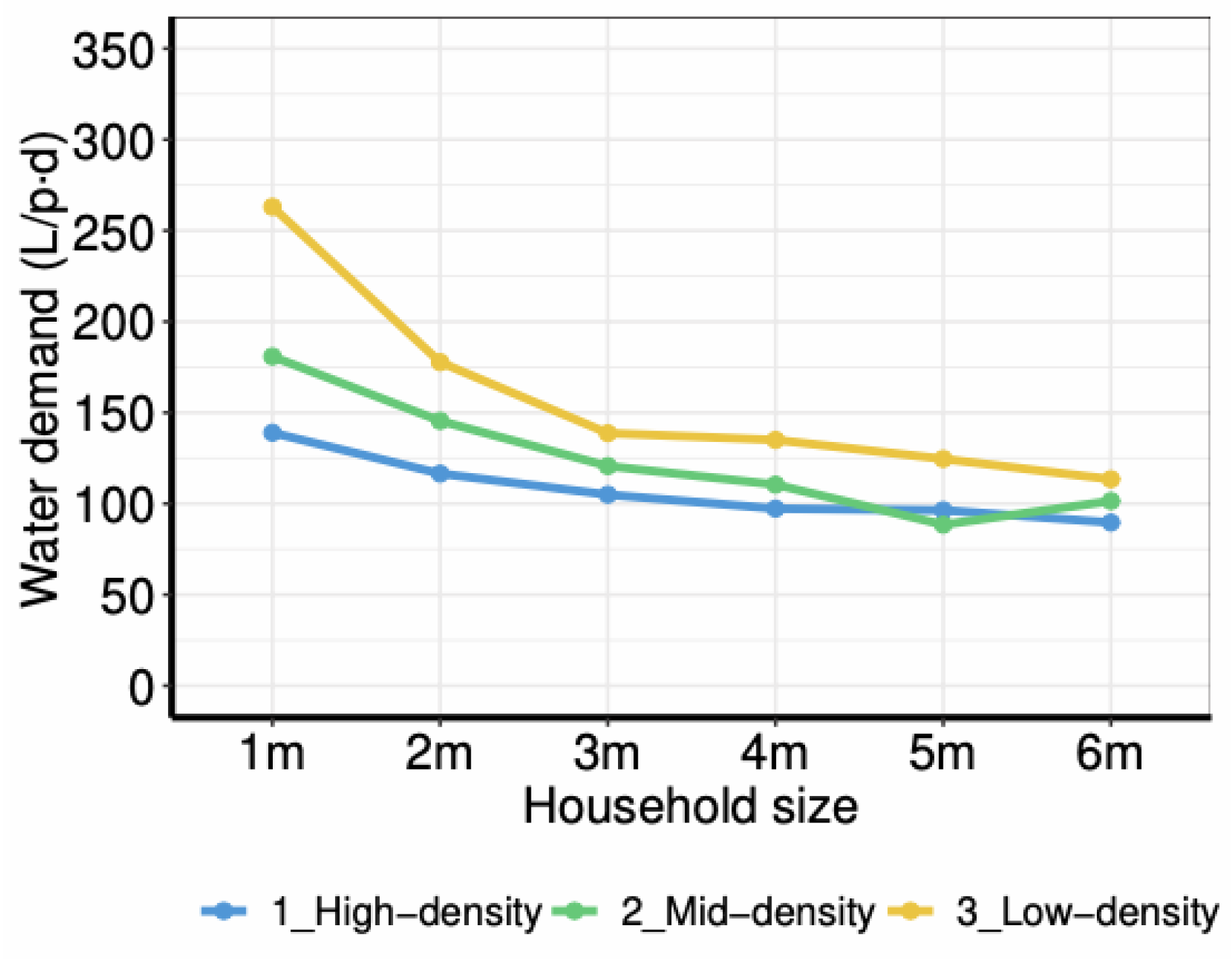
With proviso, simulating Scenario S1 reproduces some of the characteristic features observed in other works [39]. Figure 1 shows the economy of scale in water use: because water use in laundry, dishes, and maintenance benefits the whole household, regardless of the number of members on average, households with fewer members use more water than households with more members.
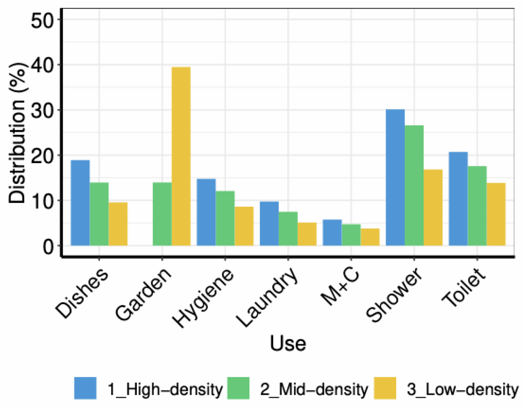
These trends are stronger for low and mid-density households, due to the water use for outdoor uses. While the difference between high and mid-density households is limited, low-density households stand out over the other housing types. In addition, the distribution of the water use among the domestic uses presents significant differences between the three housing types (Figure 2). Shower, bath and toilet represents approximately 75% of the total water use for high-density households. For low-density households, only the water use for the garden irrigation accounts for 40% of the total demand.
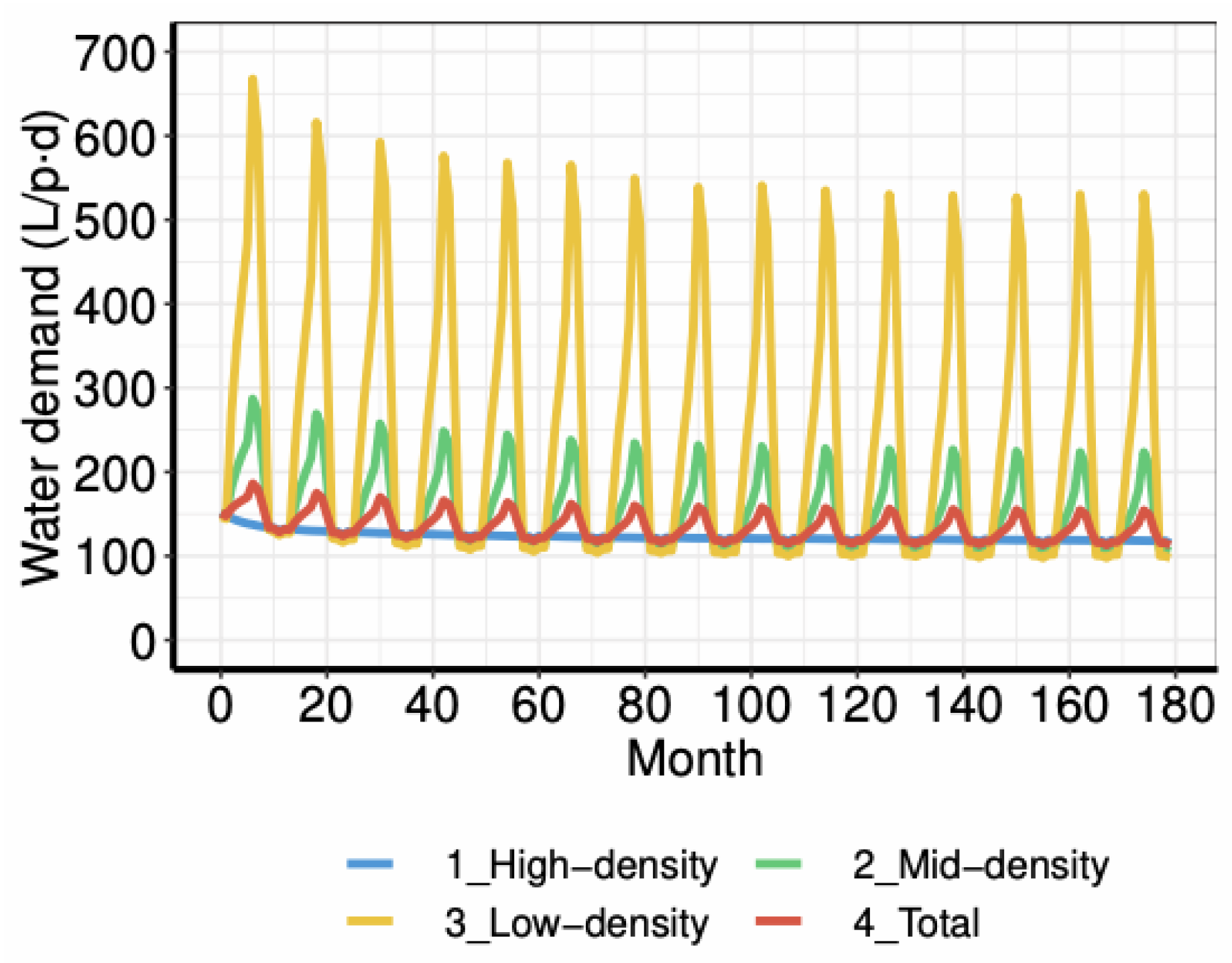
Significant differences appear for the three housing types, which are even stronger between seasons. While high-density households remain practically stable over the years, low and mid-density households exhibit demand peaks in summer due to garden irrigation (Figure 3).
4. Results and Discussion
To test the three scenarios, the model is initialised in the same way (that is, the setup is done with the same random seed and therefore the random variables are instantiated with the same values). Once the population is set up, the model takes a different seed to simulate the evolution of the state of affairs.
4.1. Scenario S1
The first scenario represents the baseline scenario, and serves to test some of the assumptions and make comparisons with other scenarios. In this scenario household sizes (i.e., number of members living in the household), housing typologies, water appliances, water fees, and citizen awareness remain stable in subsequent simulation steps. In this context, the population grows follows the description in Section 3.1.
Water use: In this scenario, per capita water use decreases over time: Households adapt to their environment taking their particularities into account (e.g., income, value profile, size) and, once they reach a satisficing outcome, they essentially do not modify their behaviour (Figure 3). At the end of the simulation, high-density households use approximately 120 L/p·day. Not surprisingly, low-density households are the ones that use a greatest volume of water, due to outdoor uses (the annual average is approximately 230 L/p·day at the end of the simulation). While in winter season their water use is low (nearly 100 L/p· day), their water use reaches 530 L/p·day in summer. Mid-density households present the same seasonal pattern (on average, 145 L/p·day over the year), although the magnitude of the peaks is limited due to their smaller gardens (225 L/p·day in summer and 105 L/p·day in winter). Taking all households into account, the average use is nearly 130 L/p·day, with peaks up to 155 L/p·day in summer (mid and low-density households’ summer use is distributed over all the population, due to the higher population of high-density households,).
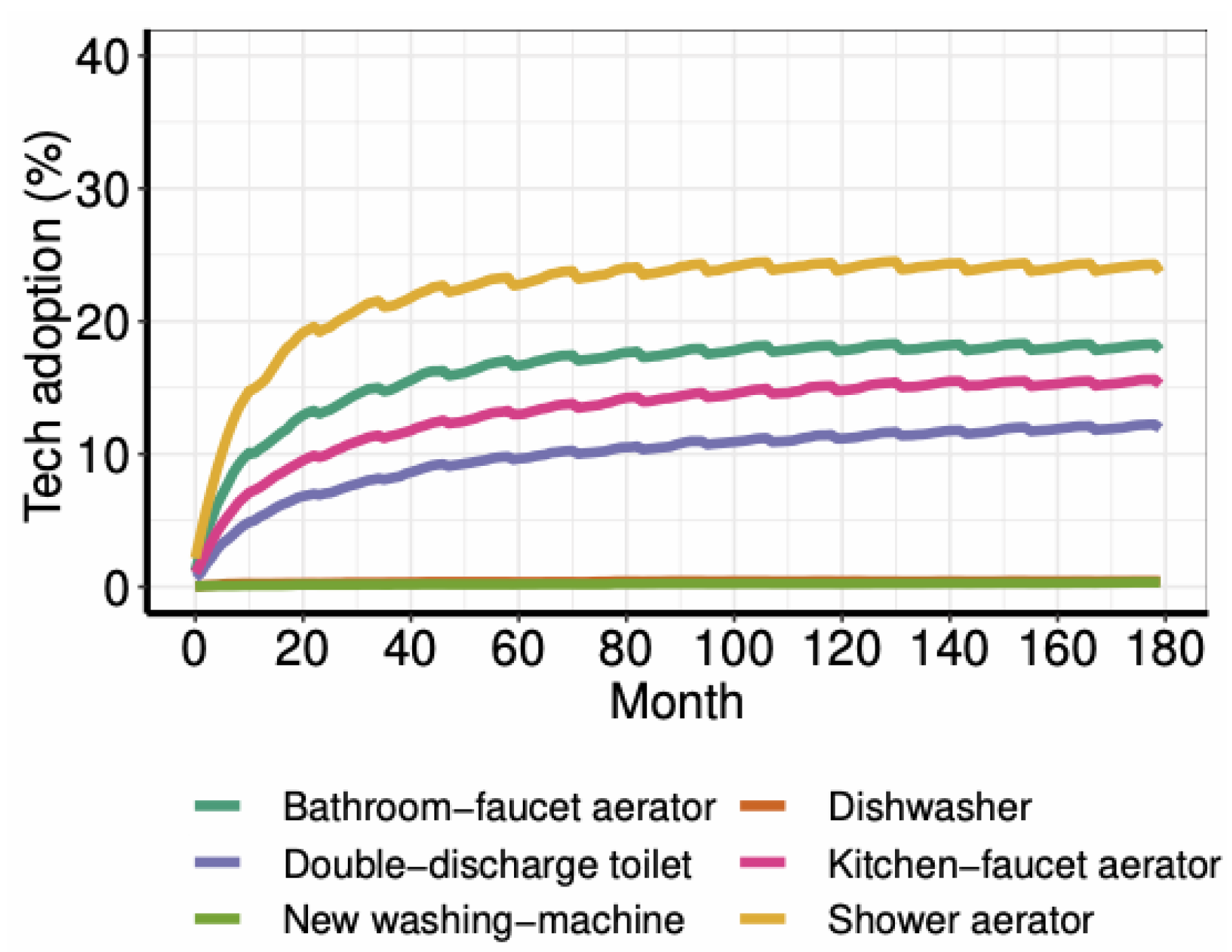
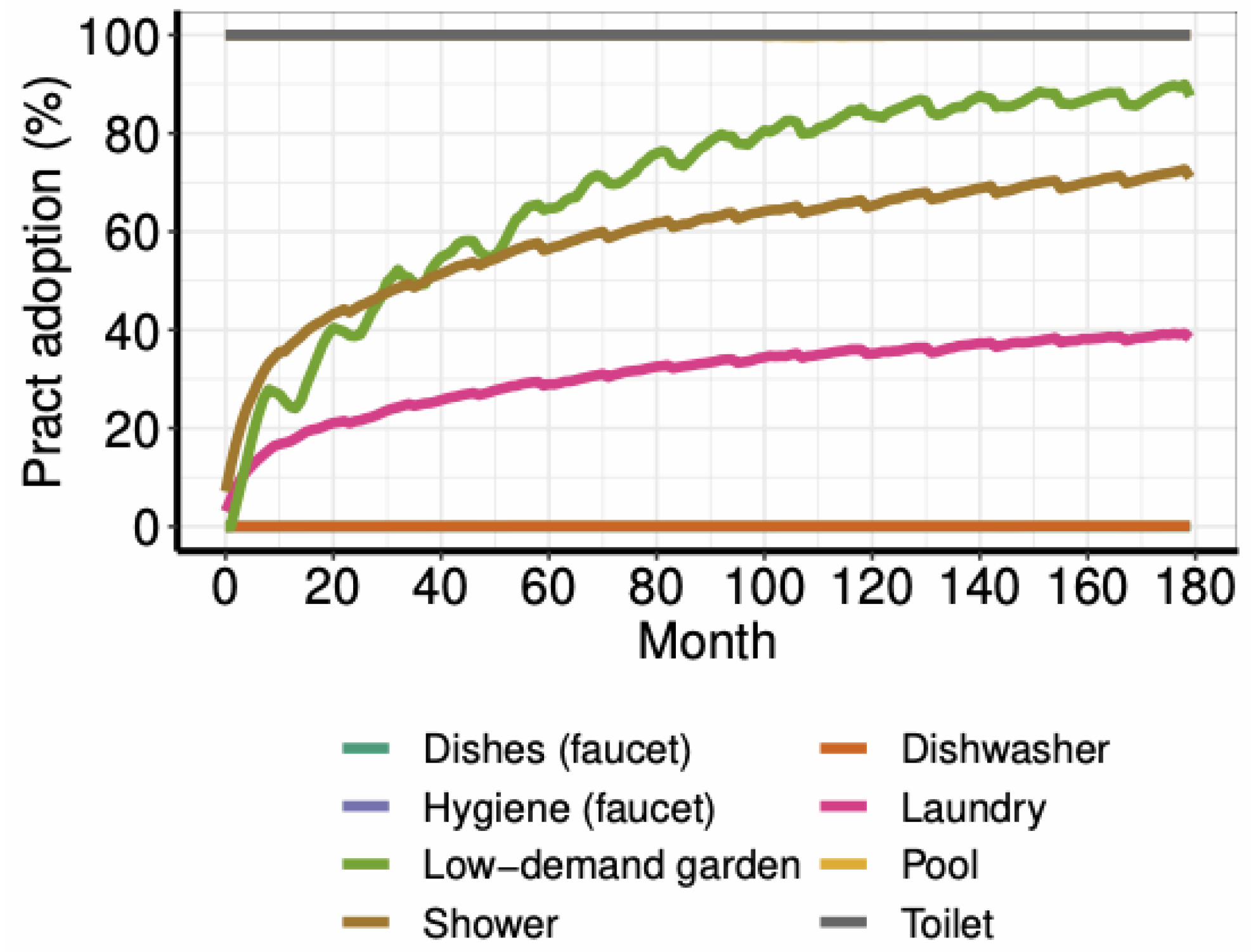
Water saving technologies and practices: Figure 4 and Figure 5 show how households adopt technologies and practices in order to adapt their water use to their particularities. On the one hand, the most adopted technologies are the shower aerator, the bathroom faucet aerator and the double-discharge toilet. The reason is their better savings/cost rate. In contrast, appliances such as new washing machines and dishwashers, in spite of saving water, are not adopted due to their cost or low savings (which suggest that these appliances are adopted for reasons outside the water realm). On the other hand, shorter showers is the practice with greatest adoption rate, followed by more austere practices in laundry and lower-use garden vegetation (90% of the households with garden end up with this practice).
The only practices that change are those related to doing the laundry, showering, and the garden vegetation. Better water-saving habits like using the dishwasher or the faucet when doing the dishes are practically not adopted (nearly 0%). Better water-saving habits with regard to the swimming pool, the toilet, and the faucet in the bathroom are maintained over time (100% of households keep the high-efficiency practices they start with). Notice that the adoption rate for low-demand garden vegetation is referred to mid and low-density households.
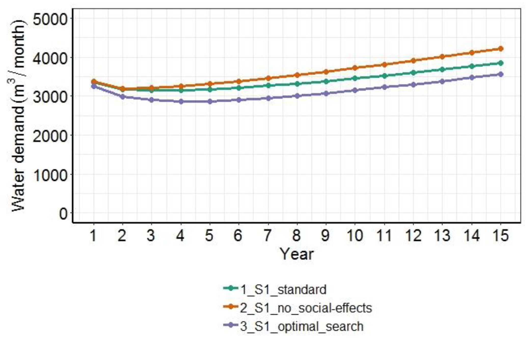
Social influence and the way households look for new practices and technologies to adopt (see Appendix A) affect the outcome of the scenario (as shown in Figure 6 and Figure 7).
On the one hand, when social influence does not occur, water use per capita is higher than the standard scenario, reaching 140 L/(p·day) at the end of the simulation. The reason is that efficient practices do not diffuse through the social network. Since many households remain within a satisficing state (either because their water bills are not expensive enough or their water use is not high enough) in the standard conditions, they do not initiate the adoption process on their own. Thus, the fact that other households start adopting practices, leads to some diffusion through the social system because of imitation.
On the other hand, if households can perform an optimal search (that is, they do not waste time looking for an innovation to outperform their already efficient behaviour), the water demand per capita is lower than the standard scenario, reaching a water use of 120 L/p·day. Interestingly, while adoption rates of practices is quite higher, this affects negatively to the adoption of technologies negatively. Because in this model it is easier to adopt practices (given that they are cost free) and since practices can be easily spread due to social effects, household reach satisficing states “earlier” due to their habits, which prevents them from assessing technologies.
4.2. Scenario S2
In this scenario, household sizes decrease and housing typologies show an important increase of small flats, as recent socio-demographic trends show [8]. Furthermore, water fees rise, as well as environmental awareness and the use of efficient water appliances (these technologies are mandatory in new housing since 2006 in Spain, so households already have them when moving to a house built after that year).
The model is initialised as discussed in Section 3.3., but the population changes specific for this scenario are: New households move to a high-density housing, start with the most efficient technology (except for doing the dishes, for which they have a faucet aerator and not a dishwasher), and have an environmentalist value profile. These new households only have 1 or 2 members (probabilities are distributed according to the relative weights shown in Table A1). Furthermore, water fees are multiplied by 3, but the blocks are kept intact.
As expected, water use per capita decreases. As the simulation advances, there are more environmentalist households that live in high-density housing and have more efficient technology. Thus, their average water use at the end of the simulation is circa 100 L/p·day despite having fewer members (in comparison to the 120 L/(p·day) of the scenario S1). Besides, the higher water fees have an effect on mid and low-density households: All households are induced to adopt low-demand vegetation in their gardens (100% of the households with garden adopt this practice). Thus, mid and low-density households demand, on average, 130 L/p·day and 210 L/(p·day) respectively. If considering all the population, the water demand is 110 L/(p·day) on average, with peaks in summer up to 130 L/(p·day).
The results suggest a form of the so-called Jevons Paradox: While households reduce their water use per capita due to technological and socio-cultural trends, the aggregation of more households (due to the population growth) of smaller size (due to the demographic trend) losses some of the potential in water saving. The main reason is that smaller households cannot take advantage of economies of scale.
4.3. Scenario S3
In the third scenario, household sizes increase (due, for example, to immigration waves), housing typologies show a balanced distribution between large and small flats, water efficient domestic fixtures increase only slightly; water pricing and taxation decrease (due, for example, to public subsidies or more cost-efficient policies by companies and regulators), and environmental awareness remains stable.
New households move to high or mid-density houses (they are 1.5 times more likely to move to high-density housing than moving to a mid-density house) and start with the regular technology except for faucet aerators and a double-discharge toilet. New households can have any value profile, and their size is 5 or 6 members (probabilities are distributed according to the relative weights shown in Table A1). Water fees are multiplied by 0.5.
In this scenario, water use per capita also decreases in the scenario, presumably due to the evolution towards household with more members and a slight improvement in technologies. On average, high-density households use circa 110 L/(p·day) at the end of the simulation; mid-density households demand 120 L/(p·day) (90 L/(p·day) in winter and 175 L/(p·day) in summer); and low-density households use 220 L/(p·day) (95 L/(p·day) in winter and 505 L/(p·day) in summer). Taking all households into account, the average water use is circa 115 L/(p·day), with peaks in summer up to 140 L/(p·day).
The rate of adoption of practices is lower in this scenario. On the one hand, new households already start with some high efficiency technologies. On the other hand, mid and low-density households pay lower water bills, which is a weaker incentive to grow low water demand vegetation in their gardens (only 70% of the households with garden have this kind of vegetation).
4.4. Comparison Between Per Capita and Total Water Use
From now on, the average over the year is used, for a better comparison of the water use levels between scenarios.
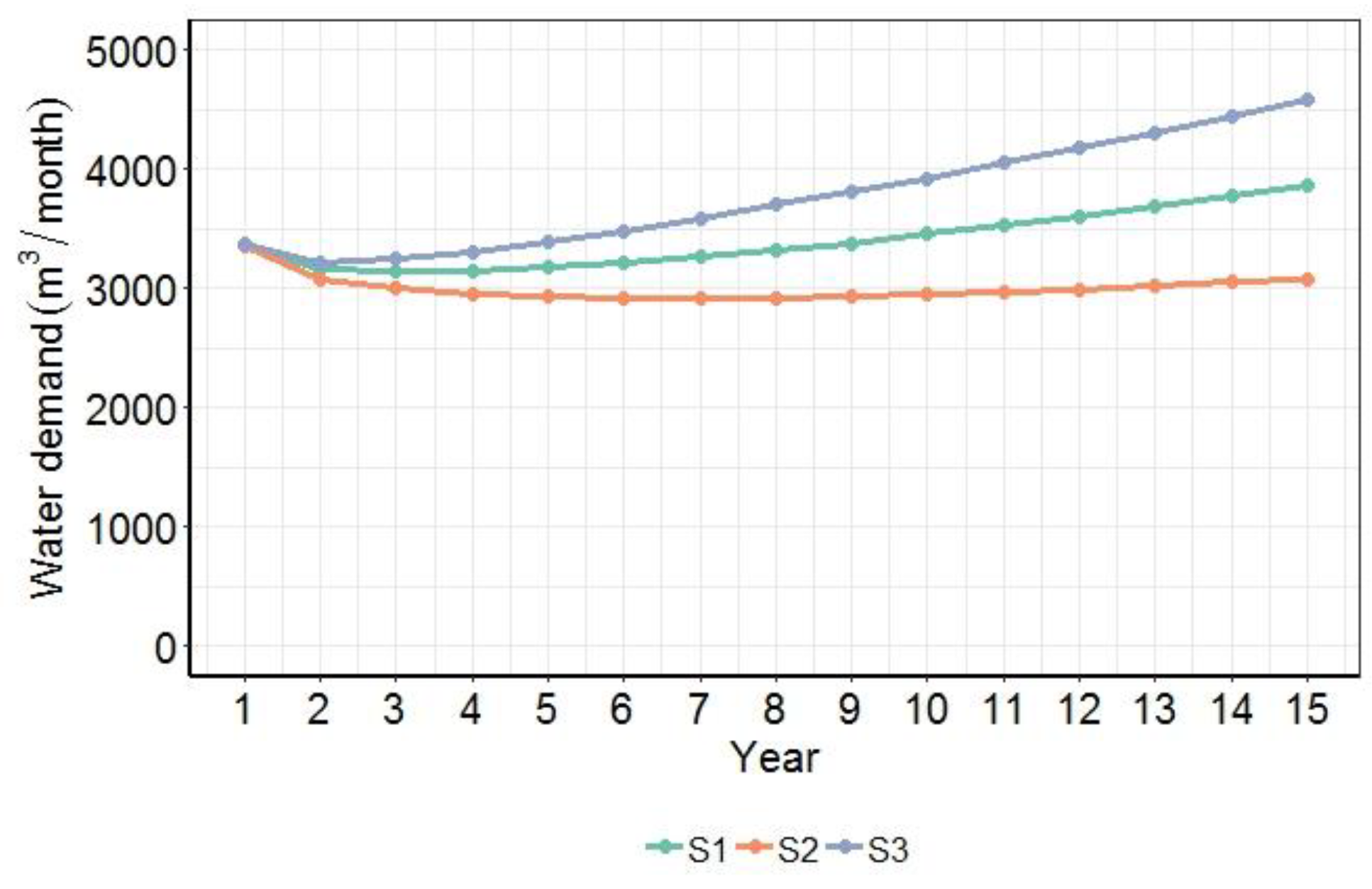
All scenarios show an increase in total water use, as expected by the population growth (Figure 8). Scenario S2 has a decreasing trend at first, showing a rising trend at the end of the simulation. The reason is that population shift towards households in high-density households equipped with high-efficiency appliances can mitigate the greater demand associated with population growth. By comparison, scenarios S1 and S3 show increasing trends from the beginning. Scenario S3 involves a higher total demand due to a greater number of newcomers.
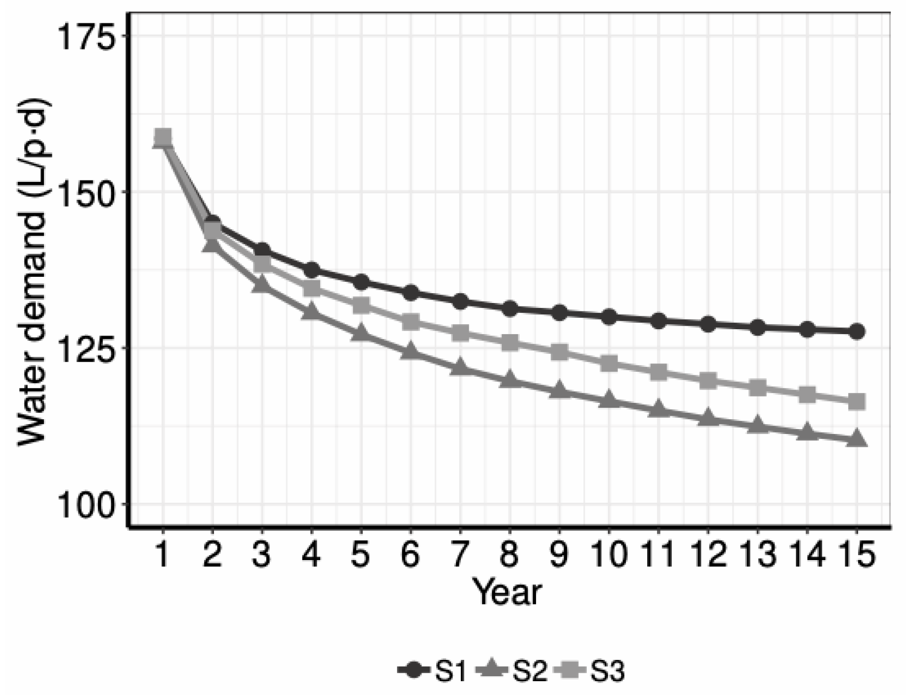
In contrast, all three scenarios present a decreasing water use per capita (Figure 9). While the scenario S3 is the one with highest total demand, it has a pronounced decrease in average demand (both caused by the growth of total population). Interestingly, if using the total demand divided by the total population as average indicator (instead of making the average of the average demand per person for each household), the result is nearly 10 L/(p·day) lower (106 L/(p·day), which contrast to the 116 L/(p·day) shown in Table 6). Scenario S2 has the strongest decrease, due to the transition high-density housing with efficient appliances (in this case, using the different average indicators does not show much difference). Since scenario S1 shows higher variation in housing types and household sizes, it also presents a higher average in water use. In this case, the difference is around 10 L/(p·day), being the first element greater than the second one.
4.5. Comparison Between Economic Impacts
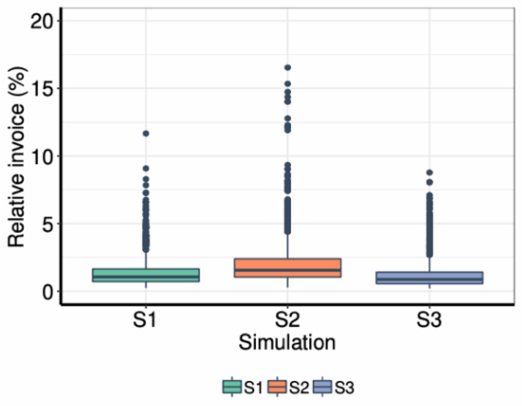
Focusing on the economic impact of the water use on the households’ budgets, scenario S2 is the one with highest impact, while scenario S3 is the one with the lowest (Figure 10). It is not surprising, since the water fees are, respectively, higher and lower than usual.
Water demand per capita decreases in all three scenarios. In the scenario S2, it decreases due to the high-efficient appliances, while in the scenario S3 it decreases because of the larger-size households. As shown in Figure 10, water bills are lower than 3% of the total budget in most households (is the proportion is higher in summer for midland low-density households). However, there are households on which the water bill causes a great impact. All simulations produce households whose invoice relative to their income is between 5% and 10%, even larger, in some simulations, and thus they are outliers of the sample, i.e., values above the third quartile plus 1.5 times the interquartile range. These households do not use much water: Often they are high-density households with a low level of income (between 3000 and 9000 EUR/year). Moreover, although the water bills are less than 2.5% of the monthly income for most of the households in all the three scenarios, there are households for which bill may exceeds a 5% of the income. In this case, the samples for each scenario are constituted of the populations of the 30 simulations altogether consequently, despite not occurring those many cases, they still appear to greater or lesser extent.
Even with a rudimentary model affordances and data sets, one may observe some aggregated behaviour that emerges from the micro-behaviours involved; yet two obvious immediate efforts can readily produce crisper insights. First, one would expect additional results will from the mere use of larger populations and larger simulation runs; second in this paper we just presented a very superficial exploitation of the model. In particular, with the current model one may draw better insights of the dynamics of water use with a more systematic analysis of the interconnections of variables. Such analysis can support some tuning of the policy measures. For instance, variations in the type and degree of social connectedness are reported only for scenario S1 and without any gradation to suggest the significance of the parameters involved. Likewise, the offsetting of household profile (household density and size, household value profile and water saving infrastructure) and water tariffs deserves a combinatorial analysis of sensitivity.
Using the current structure of the model the 5 submodels and the data classes involved (household profiles)—one may test other value-profiles, water saving activities and technologies, and different policy measures, to formulate alternative policy interventions and experiment with different scenarios to assess the effectiveness, acceptability, and value-alignment of their deployment.
5. Closing Remarks
Overview. In this paper we discuss an agent-based model to explore domestic water use in metropolitan areas under different scenarios. The purpose of the model is to illustrate the use of agent-based simulation as a tool for policy design, and more specifically to illustrate how agent-based modelling can support speculation about how policy interventions may shape plausible future situations.
The standpoint of the model is to represent relevant socio-cognitive aspects of a policy domain and its key stakeholders (like social influence, motivations and values, and cognitive heuristics) and articulate them into simulations involving population changes and policy interventions. The model focuses on households as the key decision-making unit in the case of urban water use, and combines socio-demographic variables with socio-cognitive factors deemed relevant in environmental and social psychology literature.
The parameters and variables involved in the definition of the model and the scenario definition are empirically based. Whenever possible, actual data from the metropolitan area of Barcelona is used for achieving realistic and coherent conditions.
The results of the simulations reported in the previous section, on the final aggregated and per-capita water use in the three scenarios agree with the results one can intuitively expect and the trends match results obtained with conventional equational methods. Both facts lend credibility to the results of this model. However, the purpose of our model was not forecasting the effects of demographic changes in Barcelona metropolitan area, but to visualize how the socio-cultural peculiarities of each scenario respond to very basic water saving policy interventions.
Simulations reveal that, while the increase in the number of inhabitants can lead to larger aggregated water demands, very simple policies can modulate technological and socio-cultural trends to reduce per capita water use. In some cases, the population evolution towards more households of smaller size means a loss of the potential for saving water, since smaller households do not benefit from economies of scale. Furthermore, this can exacerbate the economic impact on households with few members.
Even with the almost hands-off policies and the very crude characterisation of motivation profiles in our model, simulations hint at water saving policy interventions that deserve a more systematic analysis. Here are three obvious examples: (1) Simulations reveal that tariffs have a positive impact on aggregate water use when they become onerous for households with low occupancy; thus a steeper increment in tariff blocks may prove advisable, if politically feasible. (2) In some cases, the population evolution towards more households of smaller size means a loss of the potential for saving water, since smaller households do not benefit from economies of scale. Furthermore, this can exacerbate the economic impact on households with few members. (3) Simulations also reveal that municipal requirements that impose water saving technology adoption are obviously effective; however, their implementation and enforcement may require not only subsidies or other incentives, but elaborate campaigns. (4) Finally, the adoption of water saving practices, although dependent on the cultural profile, are susceptible to social influence. In fact, simulations show that the character of social connectedness influences in different degrees the adoption of conservation practices among households. Policymakers can use these simulation outcomes to develop strategies to enhance social learning.
The model has been based on available statistical data whenever possible, nevertheless the model includes some plausible albeit tentative assumptions. As suggested below, that points towards the need of field data and finer distinctions beyond the typical socio-demographic variables in order to avoid superfluous assumptions to support more sophisticated computational modelling. This is especially true for evidence-based policy design that better accounts for the behaviour of stakeholders.
Future work. The modest goals and achievements, as well as the acknowledged limitations of the model we presented here may be improved along these lines:
(A) Richer behaviour models: There may be considerable payoffs in sophisticating the model in two obvious directions: Cultural trends and social influence. More specifically, (1) the four cultural profiles we use are rudimentary, but they are still useful to reveal differential behaviour that affects water saving practices. More nuanced environmental behaviour can be achieved by improving the decision-making models of individual households. This can be done by building on available solid research on motivational and ethical behaviour into agent architectures that can afford planning, motivations a norm awareness [71]. (2) Likewise, the literature on adoption of innovations provides well studied mechanisms and heuristics that can be tried and tested for environmental practices and technologies [72]. In addition to their use in individuals’ decision models, this line would be especially useful for a better modelling of social influence (for instance, household heuristics for water conservation practices and richer value-responsive household profiles).
(B) Richer policy interventions. Although the current model shows the effectiveness of the use of water tariffs and water-saving requirements for new households. The treatment of policy interventions can be improved with a sharper identification and modelling-of policy means and ends. As discussed elsewhere (e.g., [73]), for this purpose, it is useful to, first, distinguish among three types of policy instruments (change affordances in the model, introduce norms and incentives, influence stakeholders’ decision-making models); second, to identify an appropriate set of values (for individuals’ motivations and for assessing policy outcomes); and third, to associate values with actions that are afforded to stakeholders and with norms and incentives to be imbedded in the model, commit to observable value indicators, scoring and aggregation functions, both for individuals and for the policy intervention.
(C) Better data. Lines (A) and (B) impose the need for a larger class of parameters to be included in the model. Sources for their instantiation will be of different degrees of availability and reliability; but even with rudimentary data sets some simulation results may still prove useful, as suggested here. The point is that a trade-off between model definitions and quality of the data needs to be analysed with the purpose of the model in mind. If that purpose is to support serious speculation for policy design, then explicit simulation assessment criteria should allow for judicious choices of data sets vs usefulness of simulation runs.
(D) Systematic analysis. This paper aimed only to illustrate the usefulness of agent-based modelling of certain type for support of policy design. The points stressed in Remark (C) should guide the performance of a systematic analysis of the model. Such analysis involves two complementary analyses, one of the results of the simulations, another of the quality of the model. The first type should follow standard methodologies for model testing, the second one deserves a concise mention.
Starting with explicit assessment criteria, one should evaluate the worth of the model in three contexts: The appropriateness of the model for the ultimate task (support of policy design); the soundness of the conceptual model for revealing relevant insights; the proficiency of the implementation of the model. These limitations together are meant to support the need for a systematic analysis of any model we suggest as a line of future work in the next section-
Extensions. The model presented here is conceived as a blueprint for other policy-support agent-based models of a particular class of phenomena involving structural and socio-cognitive factors, demographic change and conventional water saving measures. We foresee three natural extensions. First, enrichening of the model as suggested in Remarks 2.(B) and (C) above. Second, although the specifics are based on the metropolitan area of Barcelona, they should be easy to adapt to other metropolitan areas that share similar urban and social structures. Third, adaptation to other types of urban setting (beyond domestic water use and to other types of cities) may require a more thorough adaptation of behaviour and social influence models, as well as a different model for water related infrastructure and policy interventions. Nevertheless, the same blueprint should serve as a guide for the direction and depth of the adaptations. Finally, the blueprint should serve as prototype model architecture for other environmental policies where the analogous socio-cognitive, demographic, and environmental measures are characteristic. This additional function as a prototype would then become a goal in model design for the extensions suggested in remarks 2.(B) and (C), and validated according to Remark 2.(D)
Agent based modelling for policy design. We have stressed that the intended function of the model presented here is to support policy design and we have drawn attention to the usefulness of supporting serious speculation about nonconventional scenarios. The reason is that such scenarios may include features that are out of ordinary models but whose inclusion in the model suggest significant effects, and for which some policy measures, in the model, may appear appropriate. Provided a sound analysis of the model is performed (along the lines suggested in Remark 2.D) it can be used to contrast and negotiate alternative policy interventions.
An added interest for the type of model we propose is that it is based on empirical data and may thus constitute a proficient tool for the design, negotiation and monitoring of evidence-based policy.
Author Contributions
Conceptualization, A.P.-M., P.N., M.P., D.S., L.A.P.; Methodology, A.P.-M., P.N., D.S., M.P.; software, A.P.-M.; validation, A.P.-M., P.N., D.S., M.P.; formal analysis, A.P.-M.; investigation A.P.-M., P.N., M.P., D.S. and L.A.P.; resources, M.P., P.N.; data curation, A.P.-M., P.N., D.S.; writing—original draft preparation: A.P.-M., M.P., P.N., D.S., L.A.P.; writing—review and editing, A.P.-M., P.N., M.P., D.S., L.A.P.; visualization, A.P.-M.; supervision, P.N., M.P.; funding acquisition, M.P., P.N. All authors have read and agreed to the published version of the manuscript.
Funding
This research has received funding: Manel Poch wants to acknowledge Retos de la Sociedad Project (CTM2017-83598-R). LEQUIA has been recognized as a consolidated research group by the Catalan Government (2017-SGR-1552). Research by the first and fourth authors received support from the CIMBVAL project (Spanish government, project # TIN2017-89758-R) and the AppPhil project (funded by RecerCaixa 2017).
Institutional Review Board Statement
Not applicable.
Informed Consent Statement
Not applicable.
Data Availability Statement
Not applicable.
Acknowledgments
We appreciate the patience of Xisca Pericàs and her valuable help to solve all our problems regarding programming in R.
Conflicts of Interest
The authors declare no conflict of interest.
Appendix A. Submodels
Initialisation
Household size and household income attributes are set up following statistical data from the Barcelona Metropolitan Area: Household size is based on data of the province of Barcelona (INE 2013) (Table A1); while household income is based on data of the region of Catalonia (IDESCAT 2013) (Table A2). Since the annual income is given as a range, the exact income within this range is generated randomly (uniform probability distribution). This income is assumed to be distributed equally over the year, and to not change along the simulation.

Table A1.
Distribution of households according to the number of members (Source: [69]).
Table A1.
Distribution of households according to the number of members (Source: [69]).
| Number of Members | 1 | 2 | 3 | 4 | 5 | 6 |
|---|---|---|---|---|---|---|
| Distribution | 23.4 | 32.9 | 21.5 | 17.4 | 4.2 | 1.7 |
Table A2.
Distribution of households according to income and number of members (IDESCAT: [69]).
Table A2.
Distribution of households according to income and number of members (IDESCAT: [69]).
| Number of Members | <9000 | 9000–14,000 | 14,000–19,000 | 19,000–25,000 | 25,000–35,000 | >35,000 |
|---|---|---|---|---|---|---|
| 1 member (%) | 27.3 | 26.3 | 23.0 | 13.0 | 7.9 | 2.6 |
| 2 members | 7.7 | 12.4 | 16.6 | 20.9 | 20.5 | 22.2 |
| 3 members | 6.8 | 8.5 | 11.8 | 12.7 | 22.9 | 37.3 |
| 4 members | 7.6 | 4.4 | 8.4 | 11.5 | 25.4 | 42.7 |
| ≥5 members | 13.2 | 0.0 | 10.9 | 10.8 | 16.9 | 43.3 |
Water use
For a particular domestic use, households have an appliance or technology (e.g., a water-saving shower head whose flow is 10 L/min) and a habit or practice (e.g., have a 5-min shower). Technology is linked to a particular domestic use because it is assumed to occur in different rooms of the house (for instance, general hygiene uses a faucet in the bathroom, and doing the dishes uses a faucet in the kitchen).
The water use of a household j is calculated as (Equation (A1)):
where pi is the demand associated to the practice (Table 4) and it is the “magnitude” associated to the technology (Table 3) for a particular domestic use i (notice that the time of activities such as doing the dishes or showering represents the total time in which the tap is running. Thus, although activities are actually longer, the tap is not running all that time.) A household is afforded to use as much water as it wants, and there are no supply interruptions in the system. Values for practices and appliances for indoor uses have been estimated using multiple sources (e.g., environmental agencies’ campaigns, academic literature, and technical specifications of household appliances). More appliances and practices could be included in further updates of the model: For instance, practices’ demands could be represented by random distributions, in case of reliable data would be available.
Maintenance and direct consumption are decoupled from practices and technology because they are assumed to focus on a specific need of volume of water, rather than carrying out an activity. Direct consumption is estimated about 3 litres/(p·day)—3 litres/(p·day) are the biological requirement, but part of this amount is consumed through the water-fraction of food and part comes from bottled water (this model does not take into account virtual water, such as water contained in food). Maintenance demand is estimated about 50 litres/(hh·week) to clean and irrigate indoor plants. It is true, however, that behaviours could also affect this volume: For instance, irrigation of indoor plants or cleaning the house could spend different amounts of water, or members could drink more or less tap water.
Outdoor uses have been defined as follows. With regard to the swimming pool, ref [39] estimated that an average pool that is filled every year requires approximately 70 m3/year (considering stored water and evaporation losses). In the same work, it was reported that a pool is filled, on average, every three years. Accordingly, two practices are considered: annual filling, requiring 70 m3/(pool·year); and triannual filling, that requires 24 m3/(pool·year). These needs are assumed to be distributed equally over the year.
Garden irrigation needs have been calculated using the crop water requirements model from [74]. According to this model, the water requirement of a crop c is calculated as the reference evapotranspiration ET0,m (i.e., climatic conditions) multiplied by a crop coefficient Kc,m for each month m (Equation (A2)). In some works, a density factor is added, which ranges from 0 to 1 (it is neglected in this model.
Part of this water requirement is covered by precipitation. Effective precipitation Pe (i.e., the fraction of the total precipitation that can be used by crops) is roughly estimated as 80% of the total precipitation Pt. When the crop water requirement is not covered by effective precipitation (that is, ETc,m > Pe,m), households irrigate their gardens with an irrigation system (whose performance is assumed to be 60%) (Equation (A3)). Finally, the total demand for garden irrigation is calculated as the crop irrigation Nm multiplied by the garden area Agarden (Equation (A4)).
Values for evapotranspiration, precipitation and crop coefficients are presented in Table A3. Evapotranspiration values are taken from the data registered in Barcelona in 2019 (https://ruralcat.gencat.cat/web/guest/agrometeo.estacions, accessed on 24 April 2020), while precipitation values are the values for a normal year (http://www.aemet.es/es/serviciosclimaticos/datosclimatologicos/valoresclimatologicos?l=0200E&k=08, accessed on 24 April 2020). Crop coefficients are taken from cold-season turfgrass, which are used for calculating the water requirement of the high-demand garden. For the low-demand garden, coefficients are multiplied by 0.7, which represents that the garden combines turfgrass with other lower-demand vegetation (e.g., succulent plants).
Table A3.
Climatic conditions and crop coefficients for garden water use.
| Month | Evapotranspiration ET0 (mm) | Precipitation Pt (mm) | Crop Coefficient Kc |
|---|---|---|---|
| January | 37 | 50 | 0.61 |
| February | 51 | 43 | 0.64 |
| March | 84 | 44 | 0.75 |
| April | 87 | 53 | 1.04 |
| May | 117 | 58 | 0.95 |
| June | 117 | 30 | 0.88 |
| July | 153 | 24 | 0.94 |
| August | 157 | 41 | 0.94 |
| September | 145 | 75 | 0.74 |
| October | 99 | 91 | 0.75 |
| November | 66 | 66 | 0.69 |
| December | 43 | 46 | 0.60 |
| Average | 96 | 52 | 0.8 |
Adoption assessment
As discussed previously, adoption may be induced through a reasoned assessment, which includes a judgement about the ability of adopting successfully the innovation at issue. In this model, the adoption assessment model is inspired by the behaviour model from [60], being based on three components:
- Trigger: When the state of some variables of the agent’s environment is discrepant enough with those desired (or satisfactory) states, the agent is triggered to act or adapt its behaviour. For instance, some households may be triggered to adopt water-saving technology when the water bill is too high according to their expectations. This means that, if the situation is not discrepant enough, agents will not change their behaviour (thus exhibiting some degree of inertia).
- Motivation: It represents the contribution of the action to the agent’s motivations (in other words, the action’s benefit, utility, or rewarding value). Hence, this step implies some sort of evaluation mechanism (e.g., utility function or decision tree) to evaluate the action. For instance, purchasing a new washing machine that uses little water per load means to save money, which can be worthwhile for a household that values wealth.
- Ability: It represents the capacity of the agent to perform the action, with respect to its skills, resources, or entitlements. Also, these capacities can be related to the affordances that the system gives to perform the action [61] (that is, the features of the system that support the effective execution of some action by agents). This step also implies some sort of evaluation of the action. For instance, technologies are assessed with respect to its affordability; an obvious example is that an agent may be triggered and motivated to buy a new washing machine, but the appliance may be too expensive. These cognitive processes are implemented as follows: Once the agent’s trigger is activated, the agent chooses one practice or technology (see below for further details about this choice) and assesses the contribution to its motivation. If this contribution is satisficing, the agent assesses the ability to adopt. These steps represent the transition from non-adopter to potential-adopter, and from potential-adopter to actual-adopter [64]. Notice that this adoption process involves a comparison between the current situation and a hypothetical situation, whose assessment is based on the agent’s values and resources. Adoption only occurs when transiting from the current situation to the hypothetical situation increases the utility (necessary but not sufficient condition).
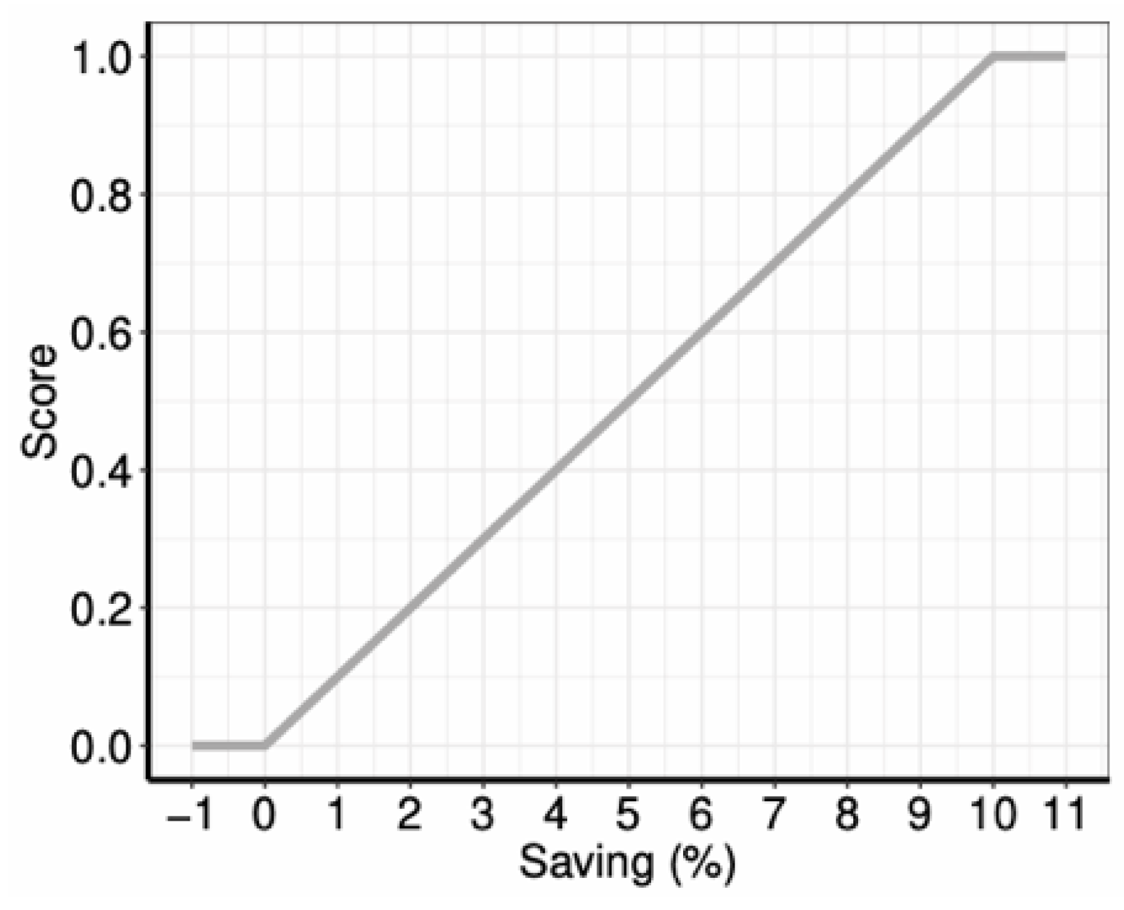
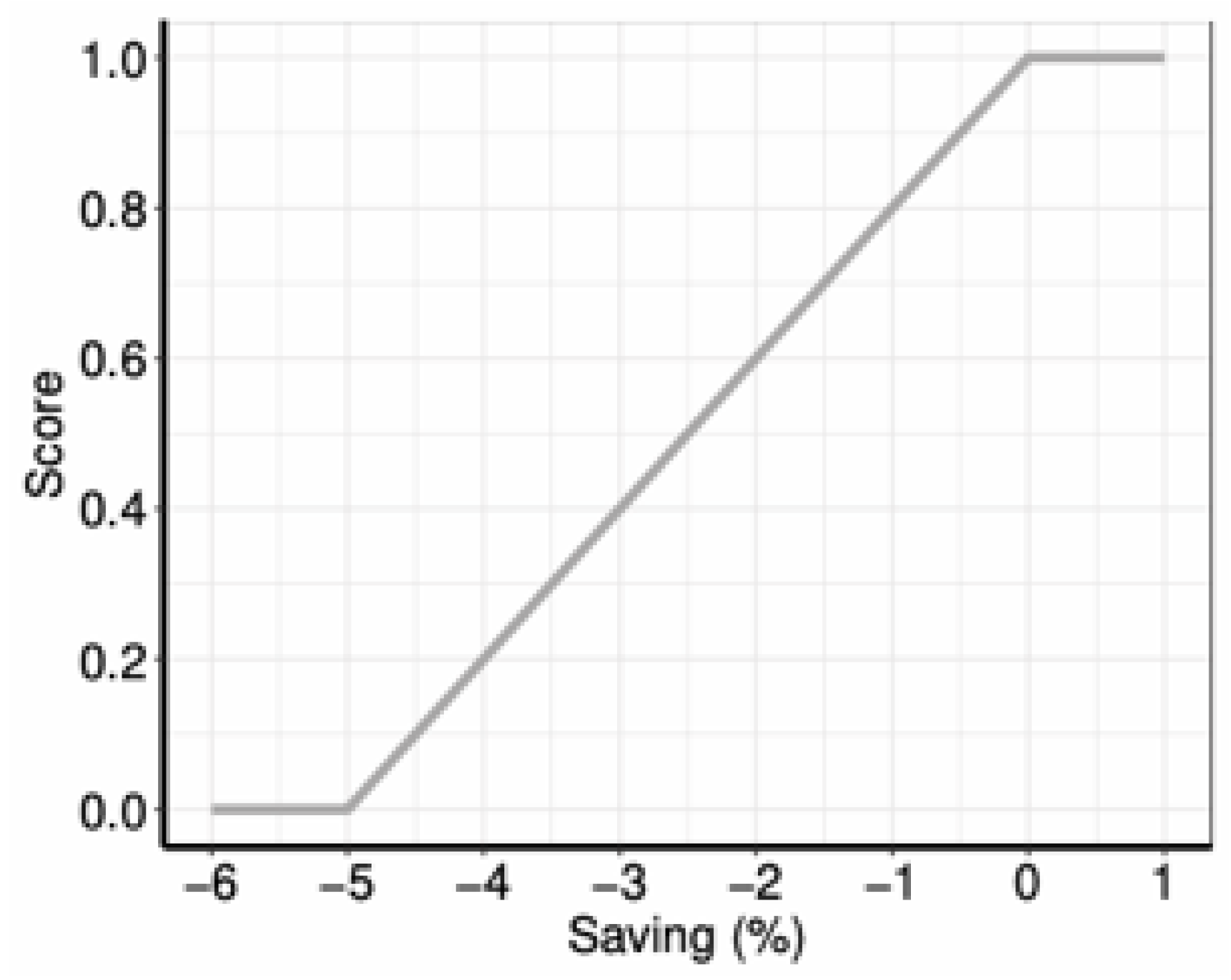
The implementation of this procedure is probability-based. Motivation is calculated by means of a utility function U that outputs a score that ranges from 0 to 1 (Figure A1). Therefore, this score can act as a success likelihood. A random number from 0 to 1 is generated then; if it is lower than the success likelihood, the household continues with the adoption process, otherwise, the adoption is immediately rejected because it is not perceived as useful. The more the practice or technology contributes to the agent’s motivations, the more likely is the agent to adopt it.
Figure A1.
Utility function to calculate the contribution of adopting a technology or practice to a household’s motivations.
Figure A1.
Utility function to calculate the contribution of adopting a technology or practice to a household’s motivations.

A similar procedure is implemented for the affordability assessment. In this model, ability is only assessed for technologies, since it is assumed that households have full control to change their habits, assumption that can be questioned if considering, for instance, the autonomy of the members within the household. Appliance adoption may be beyond the agents’ control due to their economic cost. An affordability index A is calculated (Equation (A5)), similar to other agent-based models. Accordingly, the more expensive an appliance is, the less likely is the agent to adopt it. Likewise, if the water bill is high, the agent is less likely to adopt the appliance because it subtracts economic capacity to the agent. The index ranges theoretically from 0 (total capacity to adopt) to infinite (expenses are much heavier than resources). It is assumed that an index greater than 20 prevents the household from adopting the technology. A random number from 0 to 20 is generated; if it is greater than the index, the household eventually adopts.
According to these probability-based implementations, households can fail and make “irrational” choices. For instance, a household can reject a practice that contributes greatly to their motivation, but can eventually adopt a technology that contributes little to one’s motivations and that is highly expensive. However, such cases are unusual.
As mentioned before, agents compare the current situation with a hypothetical situation to decide whether to adopt or not. This hypothetical situation is created by updating the current situation with a new practice or technology. The search procedure is relevant and reflects the cognitive skills of the agent.
It is well known that human beings are rationally bounded [75] and use multiple cognitive heuristics and are affected by several biases [76]. In a more practical way, this means that human beings look for satisficing solutions (i.e., suboptimal, but satisfactory) rather than optimal solutions, without considering all possible options. In the model, this is reflected as follows: The household chooses one random domestic use (probabilities are uniform) and then a practice or technology. For instance, a household may choose “shower” as domestic use, for which it will assess a particular practice or technology. The likelihood to choose between practices or technologies depends on the value profile (Table A4). Since in this model the set of options is limited, the household will always evaluate the option that it is not yet adopted (except in appliances for dishes, in which there are three options). Households are assumed to know about all options from the beginning, either practices and appliances that is, they can choose and assess any practice or technology, and know how to adopt them (the first assumption will avoid the typical S-shaped adoption curves, because the knowledge about innovation existence will not diffuse through the social network). Notice that households are not always “competent”: If a household has the most efficient technology and practice in a particular domestic use, they can still choose that use (thus, it is not an “optimal search”). This means that, although the trigger is activated, they can fail, because they cannot find anything more satisfying with respect to their motivations. For the sake of simplicity, mid-density households are able to change their outdoor practices on their own if they want. However, as actual mid-density households usually share a communal garden and a communal swimming pool, changing outdoor practice would probably involve agreement between all the involved households.
Table A4.
Adoption process parameters according to value profile.
| Profile | Trigger | Probability (pract : tech) | Motivation |
|---|---|---|---|
| Client | 1.5 · ΔD/B > 3% | (0.2 : 0.8) | U (1.5 · ΔD/B) |
| Techno-optimist | 2 · ΔD/B > 4% | (0 : 1) | U (2 · ΔD/B) |
| Committed | D > 140 L/p·day | (0.5 : 0.5) | U (ΔD/D) |
| Environmentalist | D > 120 L/p·day | (1 : 0) | U (ΔD/D) |
Note: D is the water demand, ΔD is the water saving and B is the water bill. U refers to the function from Figure A1.
Abandonment assessment
One difference between technologies and practices in this model is that the first cannot be abandoned. Households can be triggered to abandon practices and then activate a reasoned process in which they assess whether the abandonment of an efficient practice is acceptable (i.e., the increase in the water bill or in water use is tolerable). The abandonment assessment process is similar to the adoption assessment process. If the trigger is activated, households assess whether the utility loss is tolerable which depends on the value profile of the household (Table A5 and Figure A2 and Figure A3). Notice that this reveals that households have some values that are not explicitly modelled in the process: Because households are able to abandon “better” practices, they also value hedonism and convenience (for instance, a larger shower provides more satisfaction, although not reflected by any variable in the model, and it is acceptable as long as the increase in water use can be tolerated). Environmentalist households cannot abandon practices. This mechanism is assumed to capture the Jevons paradox: If efficient appliances are adopted (leading to lower water use and lower water bills), the abandonment process of efficient habits may be triggered, which can eventually lead to increase water use).In this case, in order to avoid that the abandonment process lead to the adoption of efficient practices, households cannot choose domestic uses in which they already have the least efficient practice, which increases the likelihood to choose other domestic uses. This is easy to understand: in actual terms, agents are not deliberately looking for an action to use more water or to increase their comfort; rather, they are losing their motivation to make that extra effort, which is implemented by retrieving one least efficient habit to test against the practice they hold.
Table A5.
Abandonment process parameters according to value profile.
| Profile | Trigger | Motivation |
|---|---|---|
| Client | 1.5 · ΔD/B < 1% | Ua (1.5 · ΔD/B) |
| Techno-optimist | 1.5 · ΔD/B < 1% | Ua (1.5 · ΔD/B) |
| Committed | D < 100 L/p·day | Ub (ΔD/D) |
| Environmentalist | - | - |
Figure A2.
Utility function to calculate the motivation when abandoning practices for client and techno-solutionist households. This lineal function maps money savings relative to water bill to a score. Notice that abandoning more efficient practices produces negative variations. If variation of the cost is high, the utility to abandon the practice is null; in contrast, if abandoning the practice does not change the situation, it leads to the maximum score. This means that, with the same water bill, households prefer to use more water (which reflects a value, although not being explicitly modelled).

Figure A3.
Utility function to calculate the motivation when abandoning practices for committed and environmentalist households. This lineal function maps the water-saving loss (i.e., variation in water use) to a motivation score. If the variation is high, the motivation to abandon the practice is null. If abandoning the practice does not change the demand of water (which is only a theoretical case), it leads to the maximum score.

Water billing
This submodel is used to calculate the water bill of households of one month, following the tariff scheme of Aigües de Barcelona (see [77]), which is the metropolitan water utility.
In general terms, the domestic water use is charged by means of two components: a fixed service fee, that depends on the housing nominal flow (e.g., 0.40 m3/h); and a variable amount, that depends on the volume of used water. Additionally, the water bill may include tributes and taxes. In this model, besides the fixed water service (Cw,fix) and the variable water use (Cw,use), a regional tribute (Ctribute) and a value-added tax of 10% are added (Equation (A6)).
It is assumed that all households have the same type of tariffs (nominal flow of 0.40 m3/h), meaning that the service-fee is 7.54 EUR/month for every household. The variable concept is based on a block tariff, which applies a progressive fee according to the volume range of water used (Table A6). The volume ranges are set for a household of three members; if the household is larger, it is possible to widen their ranges (2 m3/month per additional member in each block) (see [77]).
Table A6.
Water tariff scheme (Source: [74]).
Table A6.
Water tariff scheme (Source: [74]).
| Block | Range (m3/Month) | Price (EUR/m3) |
|---|---|---|
| 1 | [0, 6] | 0.6087 |
| 2 | [6, 9] | 1.2175 |
| 3 | [9, 15] | 1.8262 |
| 4 | [15, 18] | 2.4349 |
| 5 | >18 | 3.0436 |
The regional environmental tribute is based on the one applied by the Catalan Water Agency, which is also calculated with the blocks scheme (Table A7) (see [78]). This tribute charges at least 6 m3, in spite of the actual water use being lower, and its ranges can be widened if more than three people live in the household (3 m3/month per additional member in each block).
Table A7.
Water regional tribute (Source: [75]).
Table A7.
Water regional tribute (Source: [75]).
| Block | Range (m3/Month) | Price (EUR/m3) |
|---|---|---|
| 1 | [0, 9] | 0.4936 |
| 2 | [9, 15] | 1.1370 |
| 3 | [15, 18] | 2.8425 |
| 4 | >18 | 4.5480 |
In order to limit the model, it is assumed that households always pay their water bill, regardless of its impact on the household budget.
Social influence
In this model, social influence is based on imitation. Households can imitate their neighbours because they value conformity and stability and want to meet social expectations. This is implemented as follows: Households “observe” each of its neighbours and, if an event of probability P[imitation] = 0.10 wlink succeeds, then they will imitate a practice of a random (but common) domestic use without assessing its utility. The more similar the households (represented by the link weight wlink), the more likely it is that they imitate each other. Notice that households can imitate both less-efficient or more-efficient practices.
Additionally, households with low or mid-density housing can imitate neighbours’ outdoor practices, following the same procedure mentioned before (considering wlink =1, since households cannot know whether they share values or not).
Evolution of the population
Each year, the number of households of the system increases. According to Spanish Statistical Office, between 2001 and 2011 the number of households grew approximately 27.5% at the national level, which is an annual increase of 2.456%. New households have a random size, a random income, a random housing type and a random value profile, and start with a particular set of technologies and practices. The implementation of this submodel (e.g., probability distributions, initial technologies, initial practices) depends on the scenario at issue.
To create their social network, new households connect to a random already-existing household, and then with two of other networks of the social network of this latter household. In case these new households have mid or low-density housing, their outdoor social network consists of linking to a random mid or low-density household.
References
- Camill, P. Global change. Nat. Educ. Knowl. 2010, 3, 4. [Google Scholar]
- Rockström, J.; Steffen, W.; Noone, K.; Persson, Å.; Chapin, F.S., III; Lambin, E.; Lenton, T.M.; Scheffer, M.; Folke, C.; Schellnhuber, H.J.; et al. Planetary Boundaries: Exploring the Safe Operating Space for Humanity. Ecol. Soc. 2009, 14. [Google Scholar] [CrossRef]
- Allon, F.; Sofoulis, Z. Everyday Water: Cultures in transition. Aust. Geogr. 2006, 37, 45–55. [Google Scholar] [CrossRef]
- Tortajada, C.; Biswas, A.K. The rapidly changing global water management landscape. Int. J. Water Resour. Dev. 2016, 33, 849–851. [Google Scholar] [CrossRef]
- Milly, P.C.D.; Betancourt, J.; Falkenmark, M.; Hirsch, R.M.; Kundzewicz, Z.W.; Lettenmaier, D.P.; Stouffer, R.J. Stationarity Is Dead: Whither Water Management? Science 2008, 319, 573–574. [Google Scholar] [CrossRef] [PubMed]
- Dunn, G.; Brown, R.R.; Bos, J.J.; Bakker, K. Standing on the shoulders of giants: Understanding changes in urban water practice through the lens of complexity science. Urban Water J. 2016, 14, 758–767. [Google Scholar] [CrossRef]
- United Nations. World Urbanization Prospects: The 2018 Revision; Working Report Nº ESA/P/WP.252; United Nations: New York, NY, USA, 2018. [Google Scholar]
- Observatorio de la Vivienda en España. Las Dificultades de los Jóvenes para Acceder a la Vivienda. 2019. Available online: https://observatoriosociallacaixa.org/-/dificultades-en-el-acceso-a-la-vivienda (accessed on 24 April 2020). (In Spanish).
- Sivapalan, M.; Blöschl, G. Time scale interactions and the coevolution of humans and water. Water Resour. Res. 2015, 51, 6988–7022. [Google Scholar] [CrossRef] [Green Version]
- Gilbert, N.; Ahrweiler, P.; Barbrook-Johnson, P.; Narasimhan, K.P.; Wilkinson, H. Computational modelling of public policy: Reflections on practice. J. Artif. Soc. Soc. Simul. 2018, 21, 14. [Google Scholar] [CrossRef] [Green Version]
- Edmonds, B.; Le Page, C.; Bithell, M.; Chattoe-Brown, E.; Grimm, V.; Meyer, R.; Montañola Sales, C.; Ormerod, P.; Root, H.; Squazzoni, F. Diuerent modelling purposes. J. Artif. Soc. Soc. Simul. 2019, 22, 6. [Google Scholar] [CrossRef] [Green Version]
- Primiero, G. A Minimalist Epistemology for Agent-Based Simulations in the Artificial Sciences. Minds Mach. 2019, 29, 127–148. [Google Scholar] [CrossRef]
- Symons, J.; Alvarado, R. Epistemic Entitlements and the Practice of Computer Simulation. Minds Mach. 2019, 29, 37–60. [Google Scholar] [CrossRef]
- Aodha, L.N.; Edmonds, B. Some Pitfalls to Beware When Applying Models to Issues of Policy Relevance. In Simulating Social Complexity: A Handbook; Edmonds, B., Meyer, R., Eds.; Springer International Publishing: Cham, Switzerland, 2017; pp. 801–822. [Google Scholar]
- Parks, L.; Guay, R.P. Personality, values, and motivation. Pers. Individ. Differ. 2009, 47, 675–684. [Google Scholar] [CrossRef]
- Mair, D.; Smillie, L.; La Placa, G.; Schwendinger, F.; Raykovska, M.; Pasztor, Z.; Van Bavel, R. Understanding Our Political Nature: How to Put Knowledge and Reason at the Heart of Political Decision-Making; Publications Office of the European Union: Luxembourg, 2019. [Google Scholar]
- Achen, C.; Bartels, L. Democracy for Realists: Why Elections Do Not Produce Responsive Government. Princeton Studies in Political Behavior; Princeton University Press: Princeton, NJ, USA, 2016. [Google Scholar]
- Schwartz, S.H. Universals in the content and structure of values: Theoretical advances and empirical tests in 20 countries. In Advances in Experimental Social Psychology; Zanna, M.P., Ed.; Academic Press: Amsterdam, The Netherlands, 1992; Volume 25, pp. 1–65. [Google Scholar]
- Aarts, H. Goals, motivated social cognition and behavior. In The SAGE Handbook of Social Cognition; Fiske, S.T., Macrae, C.N., Eds.; SAGE Publications Ltd.: Thousand Oaks, CA, USA, 2012; pp. 75–79. [Google Scholar]
- Hamilton, L.C. Saving Water: A Causal Model of Household Conservation. Sociol. Perspect. 1983, 26, 355–374. [Google Scholar] [CrossRef]
- Brouwer, S.; Pieron, M.; Sjerps, R.; Etty, T. Perspectives beyond the meter: A Q-study for modern segmentation of drinking water customers. Water Policy 2019, 21, 1224–1238. [Google Scholar] [CrossRef]
- Roobavannan, M.; Emmerik THM v Elshafei, Y.; Kandasamy, J.; Sanderson, M.R.; Vigneswaran, S.; Pande, S.; Sivapalan, M. Norms and values in socio-hydrological models. Hydrol. Earth Syst. Sci. 2018, 22, 1337–1349. [Google Scholar] [CrossRef] [Green Version]
- Steg, L.; Bolderdijk, J.W.; Keizer, K.; Perlaviciute, G. An Integrated Framework for Encouraging Pro-environmental Behaviour: The role of values, situational factors and goals. J. Environ. Psychol. 2014, 38, 104–115. [Google Scholar] [CrossRef] [Green Version]
- Syme, G.J.; Nancarrow, B.E.; Seligman, C. The Evaluation of Information Campaigns to Promote Voluntary Household Water Conservation. Eval. Rev. 2000, 24, 539–578. [Google Scholar] [CrossRef]
- Owens, S. ‘Engaging the Public’: Information and Deliberation in Environmental Policy. Environ. Plan. A Econ. Space 2000, 32, 1141–1148. [Google Scholar] [CrossRef] [Green Version]
- Liu, J.; Dietz, T.; Carpenter, S.R.; Folke, C.; Alberti, M.; Redman, C.L.; Schneider, S.H.; Ostrom, E.; Pell, A.N.; Lubchenco, J.; et al. Coupled human and natural systems. AMBIO A J. Hum. Environ. 2007, 36, 639–649. [Google Scholar] [CrossRef]
- Sivapalan, M.; Konar, M.; Srinivasan, V.; Chhatre, A.; Wutich, A.; Scott, C.A.; Wescoat, J.L.; Rodrigueziturbe, I. Socio-hydrology: Use-inspired water sustainability science for the Anthropocene. Earth’s Futur. 2014, 2, 225–230. [Google Scholar] [CrossRef] [Green Version]
- O’Connell, E. Towards Adaptation of Water Resource Systems to Climatic and Socio-Economic Change. Water Resour. Manag. 2017, 31, 2965–2984. [Google Scholar] [CrossRef]
- Gilbert, G.N.; Conte, R. Artificial Societies: The Computer Simulation of Social Life; UCL Press: London, UK, 1995. [Google Scholar]
- Troy, T.J.; Pavao-Zuckerman, M.; Evans, T.P. Debates—Perspectives on socio-hydrology: Socio-hydrologic modeling: Tradeous, hypothesis testing, and validation. Water Resour. Res. 2015, 51, 4806–4814. [Google Scholar] [CrossRef]
- Gilbert, N.; Troitzsch, K. Simulation for the Social Scientist; McGraw-Hill Education: New York, NY, USA, 2005. [Google Scholar]
- Van Dyke Parunak, H.; Savit, R.; Riolo, R.L. Agent-Based Modeling vs. Equation-Based Modeling: A Case Study and Users’ Guide. In Multi-Agent Systems and Agent-Based Simulation; Sichman, J.S., Conte, R., Gilbert, N., Eds.; Springer: Berlin/Heidelberg, Germany, 1998; pp. 10–25. [Google Scholar]
- Moss, S.; Edmonds, B. Sociology and Simulation: Statistical and Qualitative Cross-Validation. Am. J. Sociol. 2005, 110, 1095–1131. [Google Scholar] [CrossRef] [Green Version]
- Galán, J.M. Evaluación Integradora de Políticas de Agua: Modelado y Simulación con Sociedades Artificiales de Agentes. Ph.D. Thesis, Universidad de Burgos, Burgos, Spain, 2007. [Google Scholar]
- Bakarji, J.; O’Malley, D.; Vesselinov, V.V. Agent-Based Socio-Hydrological Hybrid Modeling for Water Resource Management. Water Resour. Manag. 2017, 31, 3881–3898. [Google Scholar] [CrossRef]
- Mashhadi Ali, A.; Shafiee, M.E.; Berglund, E.Z. Agent-based modeling to simulate the dynamics of urban water supply: Climate, population growth, and water shortages. Sustain. Cities Soc. 2017, 28, 420–434. [Google Scholar] [CrossRef] [Green Version]
- Galán, J.M.; Del Olmo, R.; López-Paredes, A. An agent-based model for domestic water management in Valladolid metropolitan area. Water Resour. Res. 2009, 45. [Google Scholar] [CrossRef] [Green Version]
- Schwarz, N.; Ernst, A. Agent-based modeling of the diuusion of environmental innovations—An empirical approach. Technol. Forecast. Soc. Chang. 2009, 76, 497–511. [Google Scholar] [CrossRef]
- Domene, E.; Saurí, D. Urbanisation and Water Consumption: Influencing Factors in the Metropolitan Region of Barcelona. Urban Stud. 2006, 43, 1605–1623. [Google Scholar] [CrossRef]
- March, H.; Saurí, D. What lies behind domestic water use?: A review essay on the drivers of domestic water consumption. Boletín Asoc. Geógrafos Españoles 2009, 50, 297–314. [Google Scholar]
- Schulz, C.; Martin-Ortega, J.; Glenk, K.; Ioris, A.A. The value base of water governance. Ecol. Econ. 2017, 131, 241–249. [Google Scholar] [CrossRef]
- Schwartz, S.H.; Bilsky, W. Toward a universal psychological structure of human values. J. Personal. Soc. Psychol. 1987, 53, 550–562. [Google Scholar] [CrossRef]
- De Sherbinin, A.; Carr, D.; Cassels, S.; Jiang, L. Population and Environment. Annu. Rev. Environ. Resour. 2007, 32, 345–373. [Google Scholar] [CrossRef]
- Jorgensen, B.; Graymore, M.; O’Toole, K. Household water use behavior: An integrated model. J. Environ. Manag. 2009, 91, 227–236. [Google Scholar] [CrossRef] [PubMed]
- Dietz, T.; Fitzgerald, A.; Shwom, R. Environmental values. Annu. Rev. Environ. Resour. 2005, 30, 335–372. [Google Scholar] [CrossRef]
- De Groot, J.I.; Steg, L. Value orientations and environmental beliefs in five countries: Validity of an instrument to measure egoistic, altruistic and biospheric value orientations. J. Cross-Cult. Psychol. 2007, 38, 318–332. [Google Scholar] [CrossRef]
- Bardi, A.; Schwartz, S.H. Values and behavior: Strength and structure of relations. Personal. Soc. Psychol. Bull. 2003, 29, 1207–1220. [Google Scholar] [CrossRef]
- Hitlin, S.; Piliavin, J.A. Values: Reviving a Dormant Concept. Annu. Rev. Sociol. 2004, 30, 359–393. [Google Scholar] [CrossRef]
- Kenter, J.O.; O’Brien, L.; Hockley, N.; Ravenscroh, N.; Fazey, I.; Irvine, K.N.; Reed, M.S.; Christie, M.; Brady, E.; Bryce, R.; et al. What are shared and social values of ecosystems? Ecol. Econ. 2015, 111, 86–99. [Google Scholar] [CrossRef] [Green Version]
- Inglehart, R. The Silent Revolution in Europe: Intergenerational Change in Post-Industrial Societies. Am. Political Sci. Rev. 1971, 65, 991–1017. [Google Scholar] [CrossRef] [Green Version]
- Russell, S.; Norvig, P. Artificial Intelligence: A Modern Approach, 3rd ed.; Prentice Hall Press: Upper Saddle River, NJ, USA, 2009. [Google Scholar]
- Ghiassi, M.; Zimbra, D.K.; Saidane, H. Urban Water Demand Forecasting with a Dynamic Artificial Neural Network Model. J. Water Resour. Plan. Manag. 2008, 134, 138–146. [Google Scholar] [CrossRef]
- Zubaidi, S.L.; Ortega-Martorell, S.; Kot, P.; Alkhaddar, R.M.; Abdellatif, M.; Gharghan, S.K.; Ahmed, M.S.; Hashim, K. A Method for Predicting Long-Term Municipal Water Demands under Climate Change. Water Resour. Manag. 2020, 34, 1265–1279. [Google Scholar] [CrossRef]
- Rougé, C.; Harou, J.J.; Pulido-Velazquez, M.; Matrosov, E.S.; Garrone, P.; Marzano, R.; Lopez-Nicolas, A.; Castelletti, A.; Rizzoli, A.-E. Assessment of smart-meter-enabled dynamic pricing at utility and river basin scale. J. Water Resour. Plan. Manag. 2018, 144, 04018019. [Google Scholar] [CrossRef]
- Harvey, R.; McBean, E.A.; Gharabaghi, B. Predicting the timing of water main failure using artificial neural networks. J. Water Resour. Plan. Manag. 2014, 140, 425–434. [Google Scholar] [CrossRef]
- Gotts, N.M.; Van Voorn, G.A.; Polhill, J.G.; De Jong, E.; Edmonds, B.; Hofstede, G.J.; Meyer, R. Agent-based modelling of socio-ecological systems: Models, projects and ontologies. Ecol. Complex. 2019, 40, 100728. [Google Scholar] [CrossRef] [Green Version]
- Elsawah, S.; Filatova, T.; Jakeman, A.J.; Kettner, A.J.; Zellner, M.L.; Athanasiadis, I.N.; Hamilton, S.H.; Axtell, R.L.; Brown, D.G.; Gilligan, J.M.; et al. Eight grand challenges in socio-environmental systems modeling. Socio-Environ. Syst. Model 2020, 2, 16226. [Google Scholar] [CrossRef] [Green Version]
- Adamatti, D.F.; Dimuro, G.P.; Coelho, H. Making Visible “the Invisible Hand”. The Mission of Social Simulation. In Interdisciplinary Applications of Agent-Based Social Simulation and Modeling; IGI Global: Hershey, PA, USA, 2014; pp. 1–19. [Google Scholar]
- Fishbein, M.; Ajzen, I. Belief, Attitude, Intention, and Behavior: An Introduction to Theory and Research. Philos. Rhetor. 1977, 10, 130–132. [Google Scholar]
- Fogg, B. A behavior model for persuasive design. In Proceedings of the 4th International Conference on Persuasive Technology, Claremont, CA, USA, 26–29 April 2009; p. 40. [Google Scholar]
- Norman, D.A. Auordance, conventions, and design. Interactions 1999, 6, 38–43. [Google Scholar] [CrossRef]
- Lam, S.-P. Predicting Intentions to Conserve Water from the Theory of Planned Behavior, Perceived Moral Obligation, and Perceived Water Right. J. Appl. Soc. Psychol. 1999, 29, 1058–1071. [Google Scholar] [CrossRef]
- Sun, Z.; Lorscheid, I.; Millington, J.D.; Lauf, S.; Magliocca, N.R.; Groeneveld, J.; Balbi, S.; Nolzen, H.; Müller, B.; Schulze, J.; et al. Simple or complicated agent-based models? A complicated issue. Environ. Model. Sokware 2016, 86, 56–67. [Google Scholar] [CrossRef] [Green Version]
- Rogers, E.M. Diffusion of Innovations, 4th ed.; Free Press: New York, NY, USA, 1995. [Google Scholar]
- Kiesling, E.; Günther, M.; Stummer, C.; Wakolbinger, L.M. Agent-based simulation of innovation diuusion: A review. Cent. Eur. J. Oper. Res. 2012, 20, 183–230. [Google Scholar] [CrossRef]
- Burns, A.V.; Vardy, S.; Rowe, M.; Murchison, R. Victorian Water Customer: Water Services Needs & Values Summary Report; Technical Report; Accenture: Melbourne, Australia, 2011. [Google Scholar]
- Prevos, P. The Invisible Water Utility: Employee Behaviour and Customer Experience in Service-Dominant Logic. Ph.D. Thesis, College of Arts, Social Sciences and Commerce, La Trobe University, Melbourne, Australia, 2016. [Google Scholar]
- Watts, D.J.; Strogatz, S.H. Collective dynamics of ‘small-world’ networks. Nature 1998, 393, 440–442. [Google Scholar] [CrossRef]
- INE. Hogares Según su Tamaño por Estructura del Hogar, Barcelona 2011. 2013. Available online: https://www.ine.es/jaxi/Datos.htm?path=/t20/e244/hogares/p01/l0/&file=02011.px# (accessed on 8 April 2020). (In Spanish).
- IDESCAT. Nivell de Renda Anual Neta de la Llar Segons Nombre de Persones Residents a la Llar, Catalunya 2011. 2013. Available online: https://www.idescat.cat/pub/?id=ecvhp&n=6554&lang=en (accessed on 8 April 2020). (In Catalan).
- Teze, J.C.L.; Perelló-Moragues, A.; Godo, L.; Noriega, P. Practical reasoning using values: An argumentative approach based on a hierarchy of values. Ann. Math. Artif. Intell. 2019, 87, 293–319. [Google Scholar] [CrossRef]
- Perello-Moragues, A.; Noriega, P.; Poch, M. Modelling Contingent Technology Adoption in Farming Irrigation Communities. J. Artif. Soc. Soc. Simul. 2019, 22. [Google Scholar] [CrossRef]
- Perello-Moragues, A.; Noriega, P.; Popartan, L.A.; Poch, M. Modelling Policy Shift Advocacy. In Multi-Agent-Based Simulation XX. MABS 2019; Lecture Notes in Computer Science; Paolucci, M., Sichman, J.S., Verhagen, H., Eds.; Springer: Cham, Switzerland, 2020; Volume 12025. [Google Scholar] [CrossRef]
- Allen, R.G.; Pereira, L.S.; Raes, D.; Smith, M. Crop Evapotranspiration—Guidelines for Computing Crop Water Requirements; FAO Paper 56; United Nations: New York, NY, USA, 1998. [Google Scholar]
- Simon, H.A. Bounded rationality. In Utility and Probability; Eatwell, J., Milgate, M., Newman, P., Eds.; Palgrave Macmillan: London, UK, 1990; pp. 15–18. [Google Scholar]
- Kahneman, D.; Tversky, A. Choices, values, and frames. Am. Psychol. 1984, 39, 341. [Google Scholar] [CrossRef]
- Aigües de Barcelona. Precios y Tarifas. 2019. Available online: http://www.aiguesdebarcelona.cat/facturadelaigua/es/precios-tarifas/ (accessed on 16 January 2019). (In Spanish).
- Agència Catalana de l’Aigua. Canon Social del Agua. 2019. Available online: http://web.gencat.cat/es/tramits/tramits-temes/Canon-social-de-laigua-00001?category=75b0b894-a82c-11e3-a972-000c29052e2c&evolutiuTramit=1 (accessed on 16 January 2019). (In Spanish).
Figure 1.
Simulated average water use depending on the size and housing type of the household Although the three housing types show economies of scale, the low-density housing is the one that exhibits a stronger decrease in the water use per capita due to outdoor uses. Note that the shape of the curves match the shape of equational models.

Figure 2.
Simulated average water use for each domestic use depending on the housing type. The distribution of indoor and outdoor uses shows significant differences between the three housing types.
Figure 2.
Simulated average water use for each domestic use depending on the housing type. The distribution of indoor and outdoor uses shows significant differences between the three housing types.

Figure 3.
Simulated average water use for each domestic use depending on the housing type in Scenario S1.
Figure 3.
Simulated average water use for each domestic use depending on the housing type in Scenario S1.

Figure 4.
Simulated adoption of technologies in Scenario S1.

Figure 5.
Simulated adoption of practices in Scenario S1.

Figure 6.
Simulated average water use for variations of the scenario S1. Water use per capita decreases over time for all the three scenario variations. Results show that social effects contribute to reduce the water use. Likewise, if households are competent when searching for new practices and technologies to save water, water use decreases rapidly.

Figure 7.
Simulated average water use for variations of the scenario S1. All three variations exhibit an increase in the total water use because the population is growing.
Figure 7.
Simulated average water use for variations of the scenario S1. All three variations exhibit an increase in the total water use because the population is growing.

Figure 8.
Simulated total water use for the three scenarios. While the aggregated water use clearly increases in scenarios S1 and S3, it is mitigated by the social trends and housing regulations—only exhibiting a slight increase at the end of the simulation.
Figure 8.
Simulated total water use for the three scenarios. While the aggregated water use clearly increases in scenarios S1 and S3, it is mitigated by the social trends and housing regulations—only exhibiting a slight increase at the end of the simulation.

Figure 9.
Simulated average water use for the three scenarios.

Figure 10.
Simulated invoice relative to the household income for the three scenarios.

Table 1.
Household attributes.
| Attributes | Instantiation |
|---|---|
| Income (EUR/year) | [3000, 80,000] |
| Size (members) | [1, 6] |
| Housing type | High-; Mid-; or Low-density |
| Value profile | Client; Techno-optimist; Committed; Environmentalist |
| Water technology | See Table 2 and Table 3 |
| Water practices | See Table 4 |
Table 2.
Main water domestic uses.
| Domestic Use | Explanation |
|---|---|
| General hygiene | Water for hygiene-related activities (e.g., washing one’s hands, brushing one’s teeth) |
| Toilet | Water for discharging (mainly) organic waste of physiologic origin |
| Doing the dishes | Water for washing and rinsing dishes and kitchenware |
| Doing the laundry | Water for washing clothes |
| Shower | Water for washing one’s hair and body |
| Consumption | Water for cooking or drinking. Many households use bottled water |
| Maintenance | Water for cleaning the house and irrigating indoor plants |
| Garden | Water for irrigating outdoor plants |
| Swimming pool | Water for filling a swimming pool and compensating evaporation losses |
Table 3.
Water technologies considered for household.
| Domestic Use | Appliance or Technology | Floor Magnitude | Cost |
|---|---|---|---|
| General hygiene | Regular faucet Faucet with aerator | 12 L/min 6 L/min | — 3 EUR |
| Dishes | Dishwasher | 15 L/t | 300 EUR |
| Laundry | Regular washing-machine New washing-machine | 100 L/t 50 L/t | — 500 EUR |
| Toilet | Regular toilet Double-discharge toilet (3/6L) | 6 L/t 4.5 L/t (avg) | — 40 EUR |
| Shower | Regular shower-head Shower-head with aerator | 12 L/min 6 L/min | — 20 EUR |
Table 4.
Water practices considered for households.
| Domestic Use | Practice or Habit | Time or Frequency |
|---|---|---|
| Shower | Low efficiency High efficiency | 6 min/p·day, 6 t/p·week 3 min/p·day, 6 t/p·week |
| General hygiene | Inappropriate use Conventional | 3 min/p·day 1.5 min/p·day |
| Toilet | Inappropriate use Conventional | 6 t/p·day 4 t/p·day |
| Dishes | Faucet, Inappropriate use Faucet, conventional Dishwasher, low efficiency Dishwasher, high efficiency | 8 min/hh·day 4 min/hh·day 2 t/hh·day 1 t/hh·day |
| Laundry | Low efficiency High efficiency | 2 t/hh·week 1 t/hh·week |
| Garden | High-demand garden Low-demand garden | See Table A3 See Table A3 |
| Swimming pool | Annual filling and maintenance Triannual filling and maintenance | 70 m3/pool·year 24 m3/pool·year |
Table 5.
Initialisation of practices and technologies of households.
| Domestic Use | Practices | Technologies |
|---|---|---|
| Shower General hygiene Toilet | High efficiency High efficiency High efficiency | Regular shower-head Regular faucet Regular toilet |
| Dishes Laundry Garden (in case) | Low efficiency Low efficiency High-demand garden | Regular faucet Regular washing-machine - |
| Swimming pool (in case) | Triannual filling | - |
Table 6.
Scenario outcomes at the end of the simulation (15 years).
| Scenario | Average Use (L/p·Day) | Average Size (Members/hh) | Total Population | Total Demand (m3/Month) |
|---|---|---|---|---|
| S1 | 128 | 2.52 | 1090 | 3860 |
| S2 | 110 | 2.54 | 965 | 3080 |
| S3 | 116 | 3.36 | 1450 | 4590 |
Publisher’s Note: MDPI stays neutral with regard to jurisdictional claims in published maps and institutional affiliations. |
© 2021 by the authors. Licensee MDPI, Basel, Switzerland. This article is an open access article distributed under the terms and conditions of the Creative Commons Attribution (CC BY) license (https://creativecommons.org/licenses/by/4.0/).
Share and Cite
MDPI and ACS Style
Perello-Moragues, A.; Poch, M.; Sauri, D.; Popartan, L.A.; Noriega, P. Modelling Domestic Water Use in Metropolitan Areas Using Socio-Cognitive Agents. Water 2021, 13, 1024. https://doi.org/10.3390/w13081024
AMA Style
Perello-Moragues A, Poch M, Sauri D, Popartan LA, Noriega P. Modelling Domestic Water Use in Metropolitan Areas Using Socio-Cognitive Agents. Water. 2021; 13(8):1024. https://doi.org/10.3390/w13081024
Chicago/Turabian StylePerello-Moragues, Antoni, Manel Poch, David Sauri, Lucia Alexandra Popartan, and Pablo Noriega. 2021. "Modelling Domestic Water Use in Metropolitan Areas Using Socio-Cognitive Agents" Water 13, no. 8: 1024. https://doi.org/10.3390/w13081024
Note that from the first issue of 2016, this journal uses article numbers instead of page numbers. See further details here.