
Principles for Distributing Infiltration-Based Stormwater Control Measures in Series


Department of Environmental Engineering, Climate and Monitoring, Technical University of Denmark, 2800 Kongens Lyngby, Denmark
*
Author to whom correspondence should be addressed.
Water 2021, 13(8), 1029; https://doi.org/10.3390/w13081029
Submission received: 6 March 2021
/
Revised: 22 March 2021
/
Accepted: 7 April 2021
/
Published: 9 April 2021
(This article belongs to the Section Urban Water Management)
Abstract
:Infiltration-based stormwater control measures are often implemented in a dispersed manner across catchments, making it difficult to assess their combined effect. This study proposes a set of principles that can guide planners in distributing stormwater control measure volumes within a catchment while maintaining the same performance as that of a single large measure at the catchment outlet. The principles are tested by setting up seven different cases, which respect and violate the principles in different ways, and by simulating their performance using continuous simulations with 41 years of data. The results show that when the principles are followed, the system performance is maintained; on the contrary, when the principles are violated, the system performance deteriorates. The principles can be very useful for green field developers who want to implement distributed stormwater control measures in series and need to document their expected effect at an early screening level. Furthermore, the principles can be used to make better simplifications of stormwater control measures in sewer system models at the catchment level.
1. Introduction
Stormwater control measures (SCMs), also known as Sustainable Urban Drainage Systems (SUDS), Low Impact Development (LID), Water Sensitive Urban Design (WSUD) and more [1], can form an important part of the urban drainage system if widespread implementation is pursued [1,2,3,4]. In a changing climate with increasing storm intensity, SCMs that remove water from existing stormwater systems are of special interest; these are typically SCMs that involve rainwater harvesting [5,6,7] or infiltration [7,8,9,10,11]. Further, SCMs may provide a range of ecosystem services to the urban environment beyond water management, such as increased biodiversity, aesthetics and microclimate regulation [8,12,13,14].
SCMs are often implemented as multiple small elements that provide the desired services through their combined effect; such systems of SCMs are often termed treatment trains or SCMs in series. Hence, it is important to understand the cumulated effect of SCMs within a catchment [8,15,16]. Such systems of SCMs greatly increase the complexity of the sewer system, and if modelled and analysed in detail, require heavy computational efforts [17,18,19,20]. Normally, stand-alone SCMs can be dimensioned using rules based on rain statistics, while the dimensioning and performance analysis of systems of SCMs generally require long-term continuous simulations [8,21,22]. There is a need for rule-based solutions that can reduce the necessity of running expensive calculations in situations where SCM performance can be predicted adequately on a theoretical basis [23].
The determination of the contributing area and the processes leading to runoff to SCMs are in practice extremely complex. Soil types, infiltration capacity, slopes and antecedent conditions all play important roles in determining the runoff from pervious areas [24,25,26,27,28]. The effect is very much dependent on local conditions [26,27] and is largest for larger rainfall events [24,28]. Hydraulic dimensioning criteria for SCMs for well-defined small catchments are mainstreamed through guidelines around the world [29,30,31]. These take into account that one can determine the local climatic, hydrologic and geological conditions well for catchments of single SCMs and use this information to choose suitable design characteristics for the SCM. All guidelines apply to SCMs downstream in a catchment, and none of the guidelines consider distribution of SCM volume among similar SCMs within a catchment. In practice, SCM implementations where several SCMs overflow to one another within a small catchment are rather common [7,8,14]. These include within-cadaster cases where infiltration-ready depressions are connected through trenches and pipes to form a series of SCMs with a very large combined return level of overflow [8,14], as well as cases on a small neighborhood scale where also stretches of pipes are necessary to connect the different SCMs [7,14]. A feature common to both types of systems is that they function independently of a sewer system and that they are constructed such that overflow from upstream SCMs is purposefully directed to SCMs further downstream.
This study proposes a theoretical set of principles that apply to the distribution of SCM volume in a smaller catchment, where the discharge rate from the catchment must be kept below a given threshold and the total SCM volume is sought to be kept at a minimum. The principles are analysed through comparison with results from long-term continuous simulations of a set of generalized cases. The results demonstrate cases of compliance and non-compliance with the principles and are used to discuss in which practical situations the principles can be of use.
2. Materials and Methods
2.1. Theory
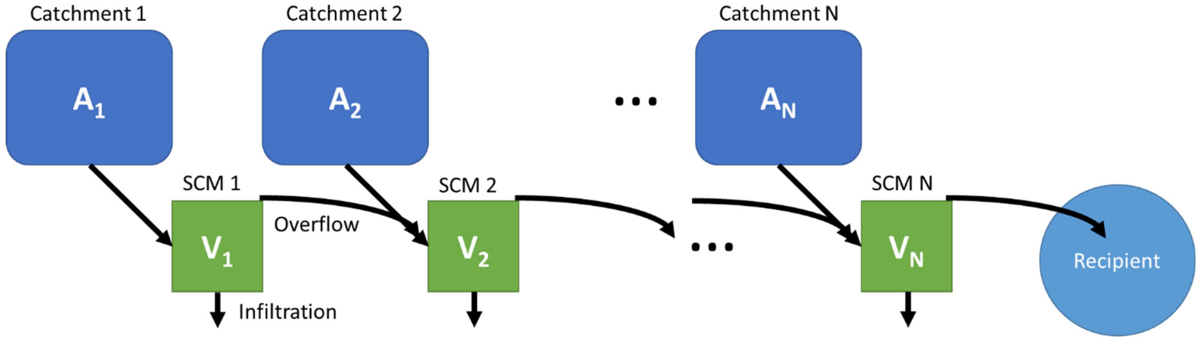
Consider a catchment consisting of multiple sub-catchments connected to SCMs as illustrated in Figure 1. Each catchment has a reduced area (An), and the connected infiltration based SCM has a volume (Vn). We do not model the pervious and impervious areas in the catchments explicitly since we are not interested in the runoff processes, but in the relative effect of the placement and sizing of the SCMs in the catchment. We denote existing methodologies for dimensioning single SCM volumes as V(A), i.e., that irrespective of the type of SCM and place in the world, local standards will use the catchment area (A) as input for dimensioning the SCM volume (V), with respect to some performance indicator such as a threshold return period for overflow [29,30,31]. Likewise, we will define the effective depth of an SCM, dn, as the volume/area ratio, dn = Vn/An, expressing how much uniform rainfall that can fall on the catchment and generate runoff into the SCM before overflow occurs. Figure 1 illustrates the sequence of N catchments with associated SCMs in series.
2.1.1. Step 1: Defining the Baseline
In the baseline case, there is only one SCM furthest downstream of the full catchment, SCM N, which is dimensioned following common practices as
indicating that the volume of SCM N is dimensioned using the combined areas of all upstream sub-catchments when it is the only SCM, as one would following common standards [29,30,31]. We use this as baseline for proposing a methodology for redistributing the volume of into a number of upstream SCMs while meeting the same performance indicator as in the baseline case.
2.1.2. Step 2: Calculating Limiting Values of Upstream SCMs
The depth parameter from the baseline, , is the limiting factor for all the upstream SCMs, and the upper limit of useful volume for any SCM, denoted n, can be defined as
indicating that all SCMs are designed for equal depth, , weighted by the relative area they serve. Additionally, the total volume should be preserved.
2.1.3. Step 3: Redistributing Volume Among SCM Elements
To achieve the same performance as in the baseline case, it is not necessary that each SCM is dimensioned to meet its baseline depth exactly. It is possible to redistribute volume from one SCM to another SCM downstream of the first SCM, as long as
stating that for all SCMs, the depth of all upstream volume over all upstream area has to be equal or below the baseline depth calculated in Equation (2), and that the total volume still needs to be the same as in the baseline case (Equation (1)).
2.2. Hypothetical Case Study
We set up a hypothetical case study including three sub-catchments in series (Figure 2). We ran continuous simulations using a rainfall time series from Kløvermarken, Copenhagen, Denmark, which is part of the rain gauge system run by The Water Pollution Committee of The Society of Danish Engineers [32,33]. The rainfall time series is identical to the one used by [8], covering 1979–2019 inclusive for this study with a time step of one minute. For each time step the following sequence of calculations was performed:
- The volume of water in SCM 1, V1, is calculated as the sum of the volume from the previous time step plus the runoff generated by multiplying the rainfall rate, R, with the area of sub-catchment 1, A1, minus the volume lost to infiltration, I1. If the calculated volume is more than the maximum volume of SCM 1, the excess is transferred to overflow, O1, and the stored volume is reduced to the maximum volume. If the calculated volume is less than zero, infiltration, I1, is reduced to balance the equation and the stored volume is set to zero.
- The volume of SCM 2 is calculated in the same way as for SCM 1, with the addition of the overflow from SCM 1, O1, to the first step as inflow.
- The volume of SCM 3 is calculated in the same way as for SCM 2 with the overflow from SCM 2, O2, replacing the overflow from SCM 1.
- The overflow from SCM 3, O3, represents the outflow from the catchment to the recipient, where we expect a threshold on the return period of outflow to apply. The frequency of overflow serves as main performance indicator for comparing the scenarios.
Eight variations of the hypothetical case study are defined in Table 1, with a varying distribution of volume among the three SCMs. In principle, the overflow frequency and volume from SCM 3 should be similar for cases 0 to 3 where the principles outlined in Equations (5) and (6) are met, whereas cases 4 and 5 should overflow more frequently as the opposite is the case. Cases 6 and 7 have larger total volume than the other cases and should lead to less overflow volume, but for case 6 a similar overflow rate, as the depth of SCM 3 is the same as in case 0. All SCMs in cases 1–7 have infiltration rates of 5 l/min, and the single SCM 3 in case 0 has an infiltration rate of 15 l/s, so the combined infiltration capacity is the same across all scenarios. Further, we choose to neglect evaporation for the simulations as it would be linearly proportional to the infiltration rates and be limited by water availability in the same manner as the infiltration.
For each case, three performance metrics are calculated for each SCM:
- The total number of calendar days where overflow occurs, nOi.
- The total volume of overflow in m3 for the duration of the simulation, VOi.
- The total volume infiltrated in m3 for the duration of the simulation, Ii.
Our main focus is the overflow volume and frequency from SCM 3, as these represent the discharge from the catchment to the recipient.
3. Results
The results of all the continuous simulations are summarized in Table 2. The results reflect the full 41 years modelled, and thus the 152 overflows reported for case 0 reflect 3–4 overflows per year.
Case 0 concentrates all volume in a single SCM, SCM 3, which is set to infiltrate at a rate that corresponds to the sum of the rates of SCMs 1, 2 and 3 in later cases. The 152 days with overflow and 4323 m3 of cumulated overflow from SCM 3 represent the best result one can achieve with 60 m3 storage volume and a total infiltration rate of 15 l/s in this hypothetical catchment. This because the full volume is placed as far downstream as possible, thus ensuring that most water is intercepted and is available for infiltration for the maximum amount of time.
In case 1, where the volume is distributed evenly between three sub-catchments, the performance of the system is exactly the same as in case 0. This is achieved by adhering to the rules defined in Equations (3) and (4), which entail that all SCMs perform alike, infiltrating and overflowing at the same rates. This is best illustrated by the overflow volumes, where the cumulated overflow from SCM 2 is the double of that from SCM 1, and the overflow from SCM 3 is the triple of that from SCM 1. This relationship arises because the overflow water from SCM 1 passes directly through the other two SCMs (and the overflow water from SCM 2 through SCM 3) as they fill up and overflow simultaneously. The fact that the infiltrated volumes are also exactly the same for all three SCMs further illustrates that the cumulated periods of time, where there is water in the SCMs, are equal.
In case 2, the volumes are distributed unevenly, with 10, 20 and 30 m3 for SCM 1, 2 and 3, respectively. According to Equations (5) and (6), this should result in the same performance as for cases 0 and 1. The results support this claim, with only four additional overflow days (+3%) and 79 m3 additional overflow volume (+2%) over 41 years of simulation. The divergence arises because more overflow occurs from SCM 1 to SCM 2 (and from SCM 2 to 3), and consequently more water is infiltrated from SCM 2 and 3, compared with case 1, as they contain water for longer periods of time. This also makes SCM 3 more vulnerable to being filled up with water from a new event before the previous event has fully infiltrated, resulting in the few additional very minor overflows compared with cases 0 and 1.
Case 3 is a more extreme version of case 2 with uneven volumes of 5, 10 and 45 m3 for SCM 1, 2 and 3, respectively. The result is also similar to that of case 2, but more extreme. The number of overflow days from SCM 3 increase to 29 (+15%) and the volume to 480 m3 (+11%) compared to case 0. Here it is evident that the smaller volumes of SCMs 1 and 2 lead to a lot more water overflow to SCM 3, and the decrease in infiltration from SCMs 1 and 2 cannot be balanced by the increase in SCM 3, thus leading to more overflows.
In cases 4 and 5, where volumes are redistributed among SCMs not respecting Equations (5) and (6) (30, 20 and 10 m3 for SCM 1, 2 and 3, respectively, for case 4 and 45, 10 and 5 m3 for SCM 1, 2 and 3, respectively, for case 5), the results are very different. More water is retained and infiltrated from SCM 1, but as the performance of SCM 2 and the even smaller SCM 3 is considerably worse than in case 0, the result is significantly more overflow days to the recipient (+229% and +705%), with the total overflow volume also increasing compared to case 0 (+30% and +136%). For both cases, the performance of SCM 1 is better than in case 1, reflecting the increased volume placed here. In case 4, the volume of SCM 2 is exactly the same as in case 1, resulting in the same number of overflows. However, the volume of overflow from SCM 2 is lower than in case 1, as SCM 2 receives less water from SCM 1 in this case, and thus has less through-flow on this account. In case 5, where the volume of SCM 2 is lower than in case 1, the performance is also worse. For both cases, the very small volumes of SCM 3 result in the overall bad performance of the system.
Cases 6 and 7 show the effect of increasing the total SCM volume by 50%. Case 6 distributes the volume “right” with increasing volumes downstream in the system (as in case 2), whereas case 7 distributes the volume among SCMs “wrongly” (as in Case 4), here resulting in the volume of SCM 3 being the same as in Case 1. For case 6, both the number and volume of overflows are reduced markedly (−54% and −46%, respectively), whereas the number of overflows in case 7 is exactly the same as for case 0, although the increased volume results in a reduced overflow volume (−38%). As such, the added 50% volume has no effect on the overflow frequency as the volume is not distributed respecting Equations (5) and (6).
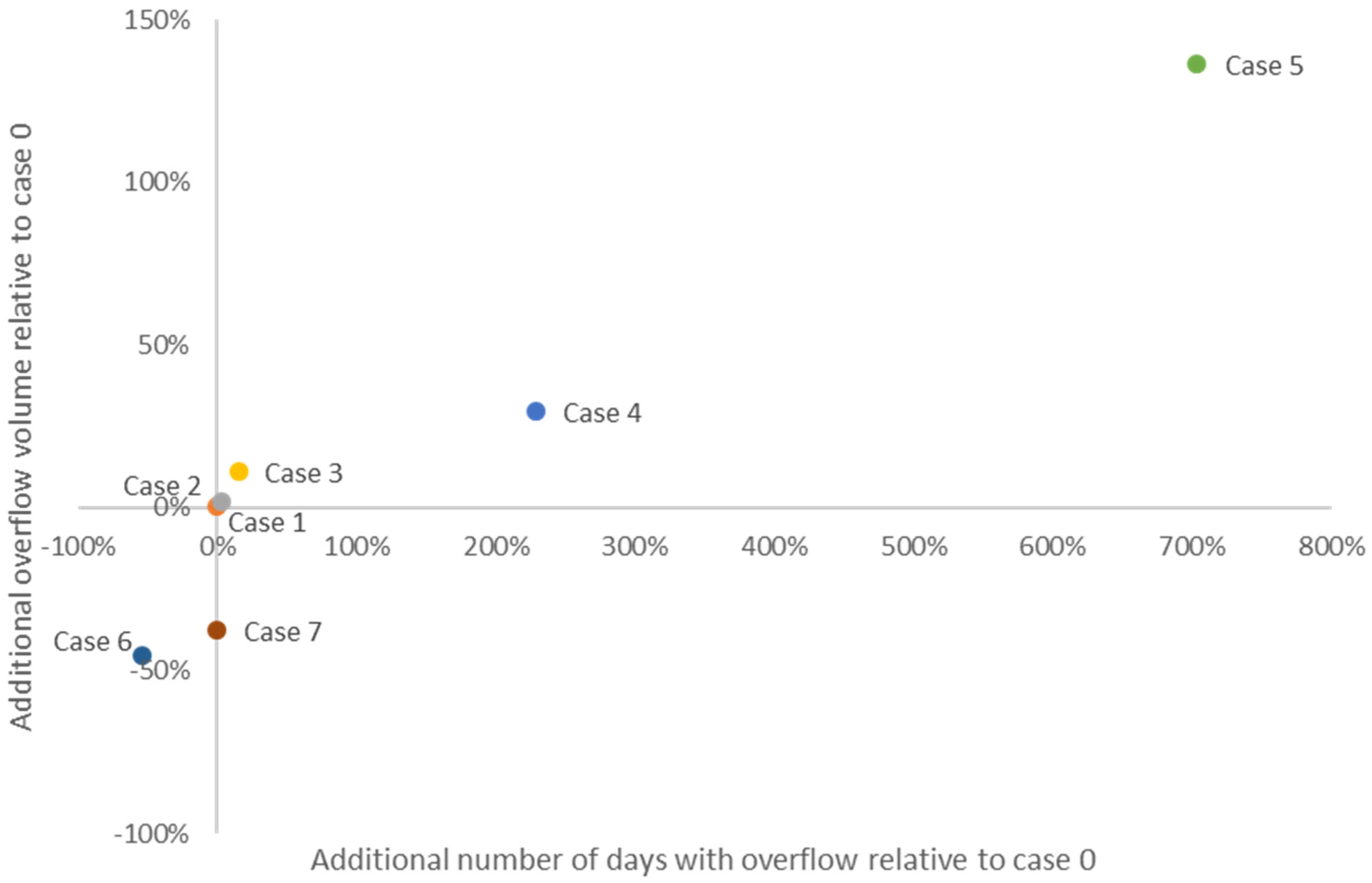
Overall, the results support the theory we propose. Figure 3 illustrates how cases 1–3 all perform very similarly to case 0, whereas cases 4–7 perform differently to varying degrees. Case 1, where the total volume of SCMs is distributed evenly (following Equations (3) and (4)), performs exactly the same as case 0, where the entire volume is concentrated in one large downstream SCM. Case 2, which redistributes the total SCM volume among SCMs following the rules of Equations (5) and (6), performs insignificantly differently from case 0. Case 3, which respects the proposed set of equations, but is very skewed in its distribution of volumes, represents a scenario where the infiltration capacity is not used optimally, leading to some divergence from case 0. Cases 4 and 5, which violate Equations (5) and (6), performs significantly worse compared with case 0. Cases 6 and 7 demonstrate that an additional 50% in total volume only leads to a smaller number of overflows if Equations (5) and (6) are respected. In case 7, where this is not the case, the performance with regard to overflow frequency is the same as in case 0.
4. Discussion
The findings are relevant in a number of practical situations.
Green-field developments are often faced with strict requirements regarding the maximal discharge rate allowed and how often this may be exceeded [33]. Technically, it is simplest to dimension and construct one SCM at the catchment outlet [29], but distributing smaller SCMs within the catchment may offer more flexibility in positioning other elements such as buildings and roads (given that the SCM does not have to occupy a large area exactly at the catchment outlet point), and other added benefits such as dispersing amenity values throughout the catchment [7,14]. In this situation, the theoretical principles we propose can be used to determine dBaseline and quickly evaluate possible solutions for distributing part of the required SCM volume into smaller SCMs upstream in the catchment. The method can also be used to quickly document that a suggested layout of distributed SCMs is likely to provide the same performance as a single large downstream SCM, dimensioned according to common standards.
The principles can easily be implemented in a map-based tool, where the user can position SCMs and give them a volume, while the tool estimates the area of the sub-catchment of each SCM (based on topography), together allowing for predicting the effective depth of each SCM and their cumulated impact.
Another situation where the principle can be beneficial is when setting up models for larger urban water systems including distributed SCMs [9,22]. Here, catchments with distributed SCMs that honour the principles in Equations (5) and (6), and behave much like cases 1 or 2, can be identified and simplified in the model to a Case 0 situation. This has the potential to greatly reduce simulation time without compromising the understanding of the real system.
The simulations of cases 0–7 build on a principle of comparable SCM volumes. For this to be true in real situation, it is of course necessary to be able to determine quite well the sub-catchment area and runoff to the individual SCMs and the drainage rate from the SCMs. Additionally, in cases where infiltration rates from different SCMs in a catchment are very different, one has to consider the fact that the volume associated with the fastest infiltration rates will in practice be more “valuable” than volume associated with lower infiltration rates. This happens as the first is more likely to drain completely between consecutive events and thus represents a larger effective volume than the latter. This could potentially be further amplified if evaporation is also considered since SCMs with larger surface areas will evaporate more than SCMs with smaller surface areas. Future research could develop the proposed principles further with weighing factors for situations where the infiltration rates vary significantly among SCMs. It could also be useful to develop rules for how much the performance of a system of SCMs will differ from the baseline given different magnitudes of deviation from the principles.
5. Conclusions
This study shows that it is possible, using the principles we propose, to distribute SCM volume within a small homogeneous catchment and predict the combined performance satisfactorily, relative to a single large SCM designed at the outlet. This is relevant as most common design guidelines address the design of single SCMs only, while in practice the implementation of SCMs in series within a catchment is relatively common. The principles are rather simple and easy to use in a “stand alone” manner and can also rather easily be incorporated into simple as well as complex design tools and modelling systems.
If the SCM volume is distributed in perfect balance within a small homogeneous catchment, the performance will be identical to the case where the full volume is concentrated at the outlet of the catchment. Cases where the volume is distributed unevenly can perform very similarly to this case if the proposed principles of distributing more volume downstream than upstream are followed. Conversely, placing more volume upstream than downstream is shown to entail worse performance with respect to the return period of overflow events and cumulated overflow volume, given an identical total SCM volume.
Author Contributions
Conceptualization, H.J.D.S. and S.M.L.; methodology, H.J.D.S. and S.M.L.; validation, H.J.D.S.; formal analysis; H.J.D.S.; writing—original draft preparation, H.J.D.S.; writing—review and editing, H.J.D.S. and S.M.L.; project administration, S.M.L.; funding acquisition, S.M.L. All authors have read and agreed to the published version of the manuscript.
Funding
This work was accomplished as part of the project SCALGO+NBS, which was supported by the Danish Ecoinnovation Program (MUDP) grant number MST-117-00555.
Institutional Review Board Statement
Not applicable.
Informed Consent Statement
Not applicable.
Data Availability Statement
The rainfall data used are a product of The Water Pollution Committee of The Society of Danish Engineers made freely available for research purposes. Access to data is governed by the Danish Meteorological Institute, and they should be contacted for enquiries regarding data access.
Conflicts of Interest
The authors declare no conflict of interest.
References
- Fletcher, T.D.; Shuster, W.; Hunt, W.F.; Ashley, R.; Arthur, S.; Trowsdale, S.; Barraud, S.; Semadeni-davies, A.; Mikkelsen, P.S.; Rivard, G.; et al. SUDS, LID, BMPs, WSUD and more—The evolution and application of terminology surrounding urban drainage. Urban Water J. 2015, 12, 525–542. [Google Scholar] [CrossRef]
- Barbosa, A.E.; Fernandes, J.N.; David, L.M. Key issues for sustainable urban stormwater management. Water Res. 2012, 46, 6787–6798. [Google Scholar] [CrossRef]
- Lerer, S.M.; Arnbjerg-Nielsen, K.; Mikkelsen, P.S. A Mapping of Tools for Informing Water Sensitive Urban Design Planning Decisions—Questions, Aspects and Context Sensitivity. Water 2015, 7, 993–1012. [Google Scholar] [CrossRef] [Green Version]
- Sørup, H.J.D.; Lerer, S.M.; Arnbjerg-Nielsen, K.; Mikkelsen, P.S.; Rygaard, M. Efficiency of stormwater control measures for combined sewer retrofitting under varying rain conditions: Quantifying the Three Points Approach (3PA). Environ. Sci. Policy 2016, 63, 19–26. [Google Scholar] [CrossRef] [Green Version]
- Jurga, A.; Pacak, A.; Pandelidis, D.; Kaźmierczak, B. A Long-Term Analysis of the Possibility of Water Recovery for Hydroponic Lettuce Irrigation in an Indoor Vertical Farm. Part 2: Rainwater Harvesting. Appl. Sci. 2020, 11, 310. [Google Scholar] [CrossRef]
- Godskesen, B.; Hauschild, M.; Rygaard, M.; Zambrano, K.; Albrechtsen, H.J. Life-cycle and freshwater withdrawal impact assessment of water supply technologies. Water Res. 2013, 47, 2363–2374. [Google Scholar] [CrossRef] [PubMed] [Green Version]
- Faragò, M.; Brudler, S.; Godskesen, B.; Rygaard, M. An eco-efficiency evaluation of community-scale rainwater and stormwater harvesting in Aarhus, Denmark. J. Clean. Prod. 2019, 219, 601–612. [Google Scholar] [CrossRef]
- Andersen, J.S.; Lerer, S.M.; Backhaus, A.; Jensen, M.B.; Sørup, H.J.D. Characteristic Rain Events: A Methodology for Improving the Amenity Value of Stormwater Control Measures. Sustainability 2017, 9, 1793. [Google Scholar] [CrossRef] [Green Version]
- Brudler, S.; Arnbjerg-Nielsen, K.; Hauschild, M.Z.; Rygaard, M. Life cycle assessment of stormwater management in the context of climate change adaptation. Water Res. 2016, 106, 394–404. [Google Scholar] [CrossRef] [PubMed] [Green Version]
- Lerer, S.M.; Righetti, F.; Rozario, T.; Mikkelsen, P.S. Integrated hydrological model-based assessment of stormwater management scenarios in Copenhagen’s first climate resilient neighbourhood using the three point approach. Water 2017, 9, 883. [Google Scholar] [CrossRef] [Green Version]
- Zhou, Q.; Panduro, T.E.; Thorsen, B.J.; Arnbjerg-Nielsen, K. Adaption to Extreme Rainfall with Open Urban Drainage System: An Integrated Hydrological Cost-Benefit Analysis. Environ. Manag. 2013, 51, 586–601. [Google Scholar] [CrossRef] [Green Version]
- Wolch, J.R.; Byrne, J.; Newell, J.P. Urban green space, public health, and environmental justice: The challenge of making cities ‘just green enough’. Landsc. Urban Plan. 2014, 125, 234–244. [Google Scholar] [CrossRef] [Green Version]
- Belmeziti, A.; Cherqui, F.; Kaufmann, B. Improving the multi-functionality of urban green spaces: Relations between components of green spaces and urban services. Sustain. Cities Soc. 2018, 43, 1–10. [Google Scholar] [CrossRef]
- Sørup, H.J.D.; Fryd, O.; Liu, L.; Arnbjerg-Nielsen, K.; Jensen, M.B. An SDG-based framework for assessing urban stormwater management systems. Blue Green Syst. 2019, 1, 102–108. [Google Scholar] [CrossRef] [Green Version]
- Bastien, N.; Arthur, S.; Wallis, S.; Scholz, M. The best management of SuDS treatment trains: A holistic approach. Water Sci. Technol. 2010, 61, 263–272. [Google Scholar] [CrossRef] [PubMed]
- Åstebøl, S.O.; Hvitved-Jacobsen, T.; Simonsen, Ø. Sustainable stormwater management at Fornebu—From an airport to an industrial and residential area of the city of Oslo, Norway. Sci. Total Environ. 2004, 334–335, 239–249. [Google Scholar] [CrossRef] [PubMed]
- Bach, P.M.; Deletic, A.; Urich, C.; Sitzenfrei, R.; Kleidorfer, M.; Rauch, W.; McCarthy, D.T. Modelling Interactions Between Lot-Scale Decentralised Water Infrastructure and Urban Form—A Case Study on Infiltration Systems. Water Resour. Manag. 2013, 27, 4845–4863. [Google Scholar] [CrossRef]
- Bach, P.M.; Mccarthy, D.T.; Deletic, A. Can we model the implementation of water sensitive urban design in evolving cities? Water Sci. Technol. 2015, 71, 149–156. [Google Scholar] [CrossRef] [PubMed]
- Löwe, R.; Urich, C.; Kulahci, M.; Radhakrishnan, M.; Deletic, A.; Arnbjerg-Nielsen, K. Simulating flood risk under non-stationary climate and urban development conditions—Experimental setup for multiple hazards and a variety of scenarios. Environ. Model. Softw. 2018, 102, 155–171. [Google Scholar] [CrossRef] [Green Version]
- Radhakrishnan, M.; Löwe, R.; Ashley, R.M.; Gersonius, B.; Arnbjerg-Nielsen, K.; Pathirana, A.; Zevenbergen, C. Flexible adaptation planning process for urban adaptation in Melbourne, Australia. Proc. Inst. Civ. Eng. Eng. Sustain. 2019, 172, 393–403. [Google Scholar] [CrossRef]
- Van Uytven, E.; Wampers, E.; Wolfs, V.; Willems, P. Evaluation of change factor-based statistical downscaling methods for impact analysis in urban hydrology. Urban Water J. 2020, 17, 785–794. [Google Scholar] [CrossRef]
- Sørup, H.J.D.; Davidsen, S.; Löwe, R.; Thorndahl, S.L.; Borup, M.; Arnbjerg-Nielsen, K. Evaluating catchment response to artificial rainfall from four weather generators for present and future climate. Water Sci. Technol. 2018, 77, 2578–2588. [Google Scholar] [CrossRef] [PubMed]
- Lerer, S.M.; Sørup, H.J.D.; Arnbjerg-nielsen, K.; Mikkelsen, P.S. A new tool for quantifying the impacts of water sensitive urban design—The power of simplicity. In Proceedings of the 10th International Conference on Urban Drainage Modelling, Mont-Sainte-Anne, QC, Canada, 20–23 September 2015; pp. 285–289. [Google Scholar]
- Sohn, W.; Kim, J.-H.; Li, M.-H.; Brown, R.D.; Jaber, F.H. How does increasing impervious surfaces affect urban flooding in response to climate variability? Ecol. Indic. 2020, 118, 106774. [Google Scholar] [CrossRef]
- Guan, M.; Sillanpää, N.; Koivusalo, H. Storm runoff response to rainfall pattern, magnitude and urbanization in a developing urban catchment. Hydrol. Process. 2016, 30, 543–557. [Google Scholar] [CrossRef]
- Penna, D.; Tromp-van Meerveld, H.J.; Gobbi, A.; Borga, M.; Dalla Fontana, G. The influence of soil moisture on threshold runoff generation processes in an alpine headwater catchment. Hydrol. Earth Syst. Sci. 2011, 15, 689–702. [Google Scholar] [CrossRef] [Green Version]
- BOYD, M.J.; BUFILL, M.C.; KNEE, R.M. Pervious and impervious runoff in urban catchments. Hydrol. Sci. J. 1993, 38, 463–478. [Google Scholar] [CrossRef]
- Davidsen, S.; Löwe, R.; Ravn, N.H.; Jensen, L.N.; Arnbjerg-Nielsen, K. Initial conditions of urban permeable surfaces in rainfall-runoff models using Horton’s infiltration. Water Sci. Technol. 2018, 77, 662–669. [Google Scholar] [CrossRef]
- Woods Ballard, B.; Wilson, S.; Udale-Clarke, H.; Illman, S.; Scott, T.; Ashley, R.; Kellagher, R. The SuDS Manual; CIRIA: London, UK, 2015; ISBN 978-0-86017-759-3. [Google Scholar]
- Melbourne Water. WSUD Engineering Procedures: Stormwater; CSIRO Publishing: Clayton, Australia, 2005; ISBN 9780643092235. [Google Scholar]
- SEMCOG. Low Impact Development Manual for Michigan–A Design Guide for Implementers and Reviewers; SEMCOG: Detroit, MI, USA, 2008. [Google Scholar]
- Gregersen, I.B.; Madsen, H.; Rosbjerg, D.; Arnbjerg-Nielsen, K. A regional and nonstationary model for partial duration series of extreme rainfall. Water Resour. Res. 2017, 53, 2659–2678. [Google Scholar] [CrossRef] [Green Version]
- Jensen, D.M.R.; Thomsen, A.T.H.; Larsen, T.; Egemose, S.; Mikkelsen, P.S. From EU Directives to Local Stormwater Discharge Permits: A Study of Regulatory Uncertainty and Practice Gaps in Denmark. Sustainability 2020, 12, 6317. [Google Scholar] [CrossRef]
Figure 1.
Illustration of N sub-catchments with associated stormwater control measures (SCMs) in series.
Figure 1.
Illustration of N sub-catchments with associated stormwater control measures (SCMs) in series.

Figure 2.
A generalized case study including three sub-catchments, three SCMs and one recipient.

Figure 3.
Relative differences in number of days with overflow and overflow volumes for cases 1–7 compared to case 0.
Figure 3.
Relative differences in number of days with overflow and overflow volumes for cases 1–7 compared to case 0.


Table 1.
Data for modelling the different cases.
| Case | A1 [m2] | A2 [m2] | A3 [m2] | Max V1 [m3] | Max V2 [m3] | Max V3 [m3] | D1 [mm] | D2 [mm] | D3 [mm] |
|---|---|---|---|---|---|---|---|---|---|
| Case 0 | 1000 | 0 | 0 | VBaseline = 60 | 0 | 0 | dBaseline = 20 | ||
| Case 1 | 20 | 20 | 20 | 20 | 20 | 20 | |||
| Case 2 | 10 | 20 | 30 | 10 | 15 | 20 | |||
| Case 3 | 5 | 10 | 45 | 5 | 7.5 | 20 | |||
| Case 4 | 30 | 20 | 10 | 30 | 25 | 20 | |||
| Case 5 | 45 | 10 | 5 | 45 | 27.5 | 20 | |||
| Case 6 | 20 | 30 | 40 | 20 | 25 | 30 | |||
| Case 7 | 40 | 30 | 20 | 40 | 35 | 30 | |||
Table 2.
Resulting performance metrics from the continuous simulations of the seven cases defined in Table 1. Percentage values in parenthesis express deviation from baseline (Case 0).
Table 2.
Resulting performance metrics from the continuous simulations of the seven cases defined in Table 1. Percentage values in parenthesis express deviation from baseline (Case 0).
| Case | nO1 [-] | nO2 [-] | nO3 [-] | VO1 [m3] | VO2 [m3] | VO3 [m3] | I1 [m3] | I2 [m3] | I3 [m3] | Total I [m3] |
|---|---|---|---|---|---|---|---|---|---|---|
| Case 0 | - | - | 152 | - | - | 4323 | - | - | 69,557 | 69,557 |
| Case 1 | 152 | 152 | 152 (+0%) | 1441 | 2882 | 4323 (+0%) | 23,186 | 23,186 | 23,186 | 69,557 (+0%) |
| Case 2 | 500 | 258 | 156 (+3%) | 3384 | 4215 | 4402 (+2%) | 21,242 | 23,796 | 24,440 | 69,478 (−0%) |
| Case 3 | 1223 | 777 | 175 (+15%) | 6456 | 9169 | 4803 (+11%) | 18,171 | 21,914 | 28,992 | 69,076 (−1%) |
| Case 4 | 68 | 152 | 500 (+229%) | 775 | 2216 | 5600 (+30%) | 23,851 | 23,186 | 21,242 | 68,279 (−2%) |
| Case 5 | 29 | 500 | 1223 (+705%) | 378 | 3762 | 10,218 (+136%) | 24,248 | 21,242 | 18,171 | 63,661 (−8%) |
| Case 6 | 152 | 106 | 70 (−54%) | 1441 | 2081 | 2354 (−46%) | 23,186 | 23,987 | 24,353 | 71,526 (+2%) |
| Case 7 | 40 | 68 | 152 (+0%) | 479 | 1254 | 2695 (−38%) | 24,148 | 23,851 | 23,186 | 71,185 (+3%) |
Publisher’s Note: MDPI stays neutral with regard to jurisdictional claims in published maps and institutional affiliations. |
© 2021 by the authors. Licensee MDPI, Basel, Switzerland. This article is an open access article distributed under the terms and conditions of the Creative Commons Attribution (CC BY) license (https://creativecommons.org/licenses/by/4.0/).
Share and Cite
MDPI and ACS Style
Sørup, H.J.D.; Lerer, S.M. Principles for Distributing Infiltration-Based Stormwater Control Measures in Series. Water 2021, 13, 1029. https://doi.org/10.3390/w13081029
AMA Style
Sørup HJD, Lerer SM. Principles for Distributing Infiltration-Based Stormwater Control Measures in Series. Water. 2021; 13(8):1029. https://doi.org/10.3390/w13081029
Chicago/Turabian StyleSørup, Hjalte Jomo Danielsen, and Sara Maria Lerer. 2021. "Principles for Distributing Infiltration-Based Stormwater Control Measures in Series" Water 13, no. 8: 1029. https://doi.org/10.3390/w13081029
Note that from the first issue of 2016, this journal uses article numbers instead of page numbers. See further details here.