
Compressor Scheduling and Pressure Control for an Alternating Aeration Activated Sludge Process—A Simulation Study Validated on Plant Data


Department of Energy Technology, Aalborg University, Niels Bohrs Vej 8, 6700 Esbjerg, Denmark
*
Author to whom correspondence should be addressed.
Water 2021, 13(8), 1037; https://doi.org/10.3390/w13081037
Submission received: 16 March 2021
/
Revised: 2 April 2021
/
Accepted: 6 April 2021
/
Published: 9 April 2021
(This article belongs to the Section Wastewater Treatment and Reuse)
Abstract
:Aiming at reducing their emissions, wastewater treatment plants (WWTP) seek to reduce their energy consumption, where a large amount is used for the aeration. The case plant, Grindsted WWTP uses an alternating aeration strategy, with a common air supply system facilitating the process in four aeration tanks and thus making optimisation challenging. In this work, a nonlinear model of the air supply system is designed, in which multiple key parameters are estimated by data-driven optimization. Subsequently, a model-based control strategy for scheduling of compressors and desired airflow is proposed, to save energy without compromising the aeration performance. The strategy is based upon partly static- partly dynamic models of the compressors, describing their efficiency in terms of system head and volumetric airflow rate. The simulation study uses real plant data and shows great potential for improvement of energy efficiency, regardless of the aeration pattern in any of the four process tanks, and furthermore contributes to a reduction in compressor restarts per day. The proposed method is applicable to other WWTP with multiple compressors in the air supply system, as this study is conducted using first principle models validated on data from the daily operation.
1. Introduction
Since antiquity, urban populations have realized the importance of good quality drinking water [1]. Yet, the significance of proper sanitation for the protection of the public health in modern cities was not realized until the nineteenth century [1,2]. Wastewater was mostly disposed of in the streets or near population centers, resulting in serious consequences for the public health and the environment [3]. This is evident by the numerous epidemics and waterborne diseases occurring throughout Europe until the nineteenth century [1,4,5]. Today, health problems associated with water pollution seem to have been almost solved by industrialized countries [1], and the focus has shifted towards waste minimization to reduce raw materials, energy and environmental releases, while simultaneously providing significant cost savings [5].
From an engineering standpoint, wastewater effluents can be made as pure as desired. However, from a practical perspective, the cost of achieving a given purity must be considered. Naturally, the most efficient way to reduce waste outputs is to reduce inputs and to make treatment processes more efficient [5,6]. The latter has been a growing topic of investigation since the late twentieth century, with the introduction of detailed simulation models and control methods for various wastewater processes [7,8,9].
The most widely used treatment process is the activated sludge process (ASP), which consists of two phases—aeration and sludge settlement [10,11]. The process was conceived in the late nineteenth century and subsequently developed into a full-scale process in 1913 [11]. Since then, the process has been widely adopted, undergone many variations and developed further, giving it a unique flexibility of operation [11].
When first modelled, the biological wastewater treatment system was passed through a sequence of events; first for modelling the removal of organic matter only, then for nitrification and lastly for nitrogen removal by biological nitrification [12]. In 1987, the activated sludge model No. 1 (ASM1) was published by the IAWQ Task Group on Mathematical Modelling for Design of Biological Wastewater Treatment [7]. Since then, the use of simulations in wastewater technology has increased [9], and dynamic modelling of the ASP has been the topic in various research [13,14,15,16,17,18,19,20,21,22,23]. Since the ASM1 was published, the IWAQ/IWA Task Group has published several other models, that add complexity to the ASP models by including additional dynamics. Namely the ASM2, ASM2d and ASM3, which all were published in the Scientific and Technical Report series by IWA Publishing and all compiled in [12]. However, the models are complex and nonlinear, difficult to fit in their parameters and validate [24,25]. For example, the simplest model, ASM1, contains 13 state variables and 19 parameters. An early attempt of improving the design and control of a continuously aerated WWTP by dynamic modelling, was conducted by two case studies in [9], where the ASM1 was calibrated and in addition; operational cost was optimized, a control strategy proposed and the feasibility of a redesign was evaluated.
1.1. The Aeration Process
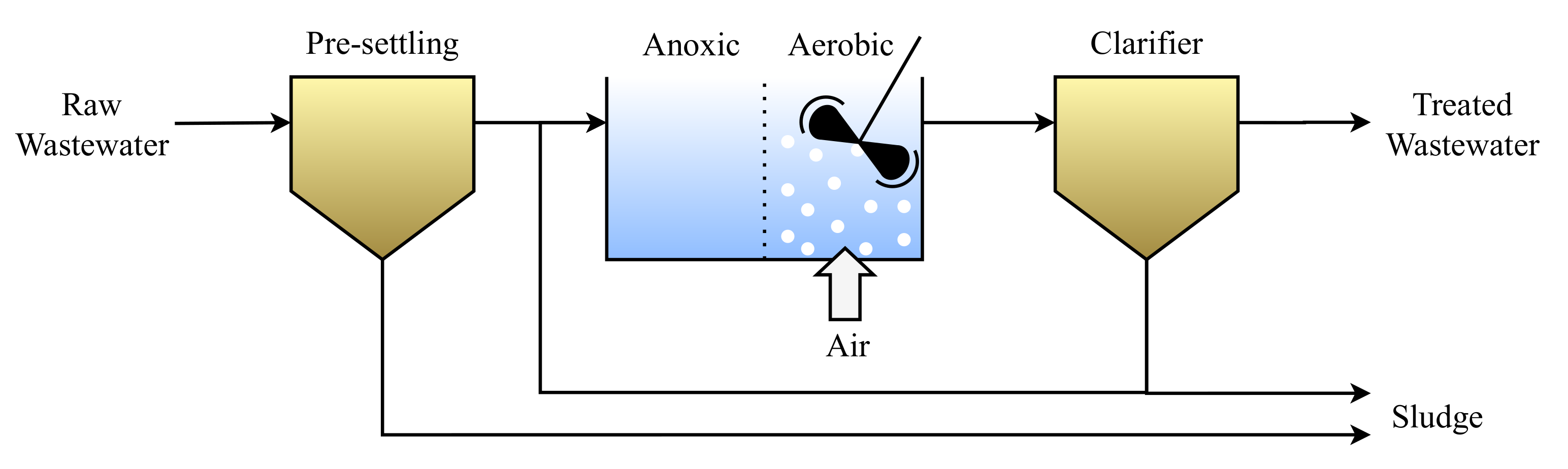
A conventional ASP is usually operated with no settlement in the aeration tank, and a completely separate settlement tank with continuous sludge removal [11]. However, in an alternating activated sludge process (AASP), the sludge is allowed to settle inside the aeration tank during anoxic treatment periods. Then aerobic treatment is facilitated by supplying compressed air, or sometimes pure oxygen, through diffusers and/or by surface agitation [11]. These treatments are also referred to as the denitrification and nitrification processes, which require anoxic and aerobic conditions, respectively. A sketch of the AASP is shown in Figure 1.
The key concept behind the AASP is that the anoxic and aerobic treatment alternates in controlled cycles to secure good treatment [26], allowing the entire nitrification/denitrification process to occur in a single tank. The aeration process is typically accomplished in large tanks, with compressors specifically sized to the hydro-static head and airflow required to facilitate aerobic treatment [18,20,27]. The compressors have to deliver large amounts of air during the aerobic cycles, consequently, the aeration process is an energy demanding process responsible for up to 75% of the total electric power demand at a WWTP [27,28,29,30]. However, electricity consumption should not be considered solely, as the discharge of nutrients is object to taxation, e.g., 30 DKK/kg discharged in Denmark [26]. Therefore, cost-analysis suggests aeration should be minimized while ensuring a satisfactory extent of nitrification [26,31]. The concept of aeration control was first introduced in the 1960’s to save energy by avoiding over-aeration in lowly loaded periods [31]. Today many WWTP’s in Denmark run the commercially available control system STAR (Superior Tuning and Reporting) [26], that changes the aeration set-point according to a rule-based control strategy from newest ammonium and nitrate measurements as described in [32,33]. The process is flexible and can adapt to different wastewater compositions by controlling the dissolved oxygen set-point and duration of aeration [26,33].
1.2. State-of-the-Art
Dynamic modelling of the wastewater treatment processes has been the topic of various research [9,13,14,15,16,17,18,19,20,21,22,23,34,35,36,37], and usually with the aim of incorporating control systems leading to improvements in the performance, or with the purpose of designing (or redesigning) WWTPs [9,36]. In [36,37], mathematical models are developed by applying material and energy balances to a process tank, and similar methods are presented in [34,35] where the aeration tank and settler are modelled in Matlab Simulink.
Especially models the dissolved oxygen (DO) dynamics has been of great interest Refs. [16,20,21,22,24], since control of the ASP based on DO measurements has the advantage of using reliable and relatively cheap sensors which are capable of measuring the DO concentration in real-time [16,38,39]. An early attempt of improving the design and control of a continuously aerated WWTP by dynamic modelling, was conducted by two case studies in [9], where the ASM1 was calibrated and both; operational cost was optimized, a control strategy proposed, and the feasibility of a redesign was evaluated.
Energy savings in the AASP have been investigated in various works [26,27,40,41]. An economic approach is used in [26,27] where predictive control is used to prioritize aeration in periods with low electricity prices. Similarly, in [41], advanced control of the aeration cycles is implemented to improve the effluent water quality, and the study shows that the optimization results in lower power consumption. In both studies, energy consumption is reduced by modifying the aeration pattern i.e., the nitrification/denitrification cycle, but the air supply system itself is disregarded. The air supply system is often glossed over when discussing optimal control of nitrogen removal in WWTP research, under the assumption that compressor dynamics are fast, and a local control loop regulates it to a dissolved oxygen (DO) set-point [14].
The alternating nature of the nitrification/denitrification cycle implies varying load conditions for the compressors; hence, the flexibility of the air supply system is crucial for the performance of the aeration system [42,43]. This is particularly true for systems where multiple aeration tanks are maintained by a single air supply unit, which will be investigated in this work. Various control strategies have been established for continuously aerated reactors (DO set-point at 2–3 mg/L) [19,31,44]. In industrial practice, the process controller usually consists of simple feedback loops, such as bang-bang control ref. [45] or Proportional Integral (PI) controllers that regulates airflow and valve position Refs. [18,24,29,44,46,47]. Commonly, the so-called “most opened valve” approach is applied in systems with multiple shared aeration tanks [18,42,44]. With this method pressure is controlled to maintain the most open valve almost completely open, to improve compressed air efficiency by reducing head-loss in the supply pipeline [18,25,44,48]. However, in an AASP the valves travel further in comparison, as each tank is not continuously aerated, but must track the aeration pattern in both DO concentration and aeration period (meaning completely closed pipelines often are present). Consequently, the air supply has to adapt to vastly changing flow demands and system pressure characteristics. This problem is reminiscent of the problem with unknown system characteristics found in Heating Ventilation and Air Conditioning (HVAC) [49,50,51,52], and optimization of compressor networks [43,53].
1.3. Objectives & Contribution
This study aims to improve energy efficiency in AASP aeration systems, while still prioritizing nutrient removal in the wastewater, and we set up a hypothesis to investigate whether the energy efficiency of the compressed air supply in an AASP can be increased without actually changing the aeration pattern and DO set-point generation and tracking. As stated in Section 1.2, the given problem statement of decreasing energy consumption is commonly addressed by modelling the biochemical processes and using these models for control and plant optimization. Contrary, we propose a novel approach where the difficulties of defining first principle biological models are bypassed/circumvented, and energy savings are obtained using data-driven models and well known methods where data from the daily operation can be used to obtain and validate models. The method we propose is hence more applicable than the commonly used approach where it is necessary to calibrate the ASMs and the wastewater characteristics must be known. To test the hypothesis, we propose a pressure controller that adapts to the changing system characteristics and an efficiency improving scheduling algorithm which ensures the compressor system runs at maximum total efficiency. The term scheduling is used throughout this work to describe the strategy which determines how many and which compressors are running, and at what load each compressor is running.
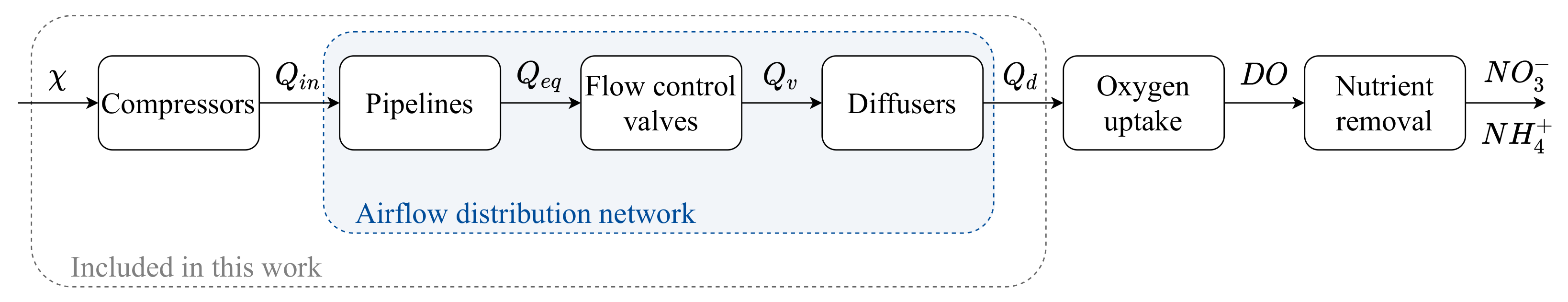
The relevant subsystems must first be modelled in order to utilize the models for controller design and scheduling improvement. Figure 2 illustrates a typical WWTP aeration system, where the input is compressor load percentage () for all compressors and output is the nutrient concentration in the wastewater. The subsystems considered in this work are marked inside the grey dashed rectangle. Note that all signals presented in Figure 2 can be one-dimensional or multi-dimensional, depending on the specific WWTP layout.
As shown in Figure 2, this work presents models for the compressors, pipelines, flow control valves and bubble diffusers at the bottom of the aeration tanks. The compressors are modelled using static methods describing the efficiency map of the compressors in terms of system head and volumetric airflow rate. The remaining three subsystems; pipelines, flow control valves and diffusers are combined and presented as the airflow distribution network (marked in Figure 2 with a blue dashed rectangle). The notation used in Figure 2 is explained in Table 1. All proposed models are tested against data from a real plant, where key parameters are optimized to increase model prediction accuracy.
In summary, this paper presents a novel strategy for compressor scheduling and control of the desired airflow to save energy without compromising wastewater quality. The proposed scheduling algorithm incorporates changing system characteristics in the selection process, to choose the optimum operation point for the compressors, which results in maximized total efficiency. Three controllers are proposed in this work: a static feedforward compensator, a classical feedback PID and a combined feedforward-feedback controller. The scheduling algorithm and the proposed control strategies are implemented and evaluated in a simulation model based on real plant data.
This paper is structured as follows: Section 2 describes the case plant and the system which is to be modelled. In Section 3, a first principle model of the airflow distribution network is presented and parameter estimation is performed to fit the model to plant data. The presented model is henceforth referred to as a simulation model based on plant data, and subsequently used to generate static system curves representing the counter-pressure which the air supplying compressors has to overcome. In Section 4 a feed-forward pressure controller is proposed and evaluated based on its performance compared to a traditional feed-back PID controller and feed-forward compensation. In Section 5, a compressor scheduling algorithm with the goal of improving energy efficiency is introduced and implemented in the simulation model, and the results are presented and evaluated in Section 6. Finally, the contribution of this work is discussed in Section 7.
2. Case Plant: Grindsted Wastewater Treatment Plant
The Grindsted wastewater treatment plant which is a part of the Billund Biorefinery (BBR), is the focus of the investigation in this work. The plant is located outside Grindsted, Denmark, and serves a catchment of 70,000 population equivalents (PE). The aeration system consists of four alternating aeration tanks connected in parallel, for which two centrifugal compressors ( and ) deliver the required airflow rate. For future reference, system parameters and measurements for individual tanks will be noted by a subscript , and the term airflow will be used when referring to the volumetric airflow rate. A schematic of the aeration system is presented in Figure 3.
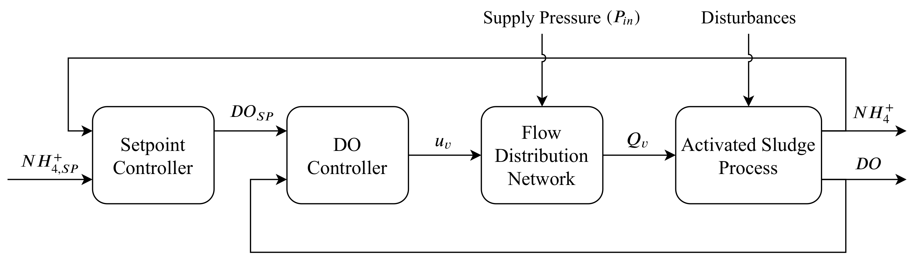
As noted in Figure 3, the airflow and DO, nitrate (NO) and ammonium (NH) concentrations are measured in each tank. Lastly, the pressure in the air supply pipe is measured upstream to the aeration tanks. The influent and effluent concentrations are unknown, as well as the volume of entering wastewater. Due to unknown wastewater inputs, as well as external conditions affecting the biochemical processes, disturbance effects are introduced in the ASP [42]. Hence, to achieve proper nitrogen removal, a system of cascaded controllers maintains the concentrations of nitrate and ammonium to desired set-points. A block diagram of the general system is shown in Figure 4.
The work is based upon measurements from the introduced sensors, as well as power readings from the individual compressors. The measurements were sampled at 15 s intervals over a period of nine consecutive days. Note that the data was acquired during normal operation of the case plant.
Seen from a control perspective, the manipulated variables i.e., the actuators, are the flow regulating valves and the compressors. A consequence of the shared air supply system is that the airflow to a specific tank is not solely dependent on the respective valve, but also on the state of the remaining valves. An analogy for this system could be made in electrical networks [54], where larger currents occur in lines with less resistance. Furthermore, as the compressors operate within a specific limit of operation in terms of head and airflow, the compressors are also coupled with the state of the valves making efficient control of the DO loop more difficult. Referring to the electrical analogy, the model describing the coupling between valves and compressors is noted as the airflow distribution network. Depending on the modelling perspective, the compressor input can be in terms of total airflow or supply pressure. The latter is used when deriving the model in later sections, hence, it is illustrated as such in Figure 4.
The disturbance input in the ASP is shown to emphasize that various factors influence the ASP e.g., time-varying parameters such as influent and effluent concentrations, pH-value and variation in the wastewater fauna [42]. The signal names introduced in Figure 4 are summarized in Table 2.
The DO control loop in the case plant is currently regulated by a rule-based strategy consisting of two main logic/control algorithms;
- Algorithm 1
- A relational operator determines which compressor to activate depending on the number of completely open valves.
- Algorithm 2
- The DO controller is a relational operator between DO feedback and set-point, meaning the valves are either set completely open or closed.
Naturally, the compressors have been designed to achieve efficient performance in a specific operating region referred to as the best efficiency point (BEP). However, when changing the system head by opening additional valves, the compressor operates further from the optimal operation point, resulting in periods with inefficient aeration [42]. This control scheme may further deteriorate the lifespan of the compressors that have to accommodate to frequent changes in system head and have to shut off entirely in intervals where few or no valves are completely open.
3. Modelling of the Airflow Distribution Network
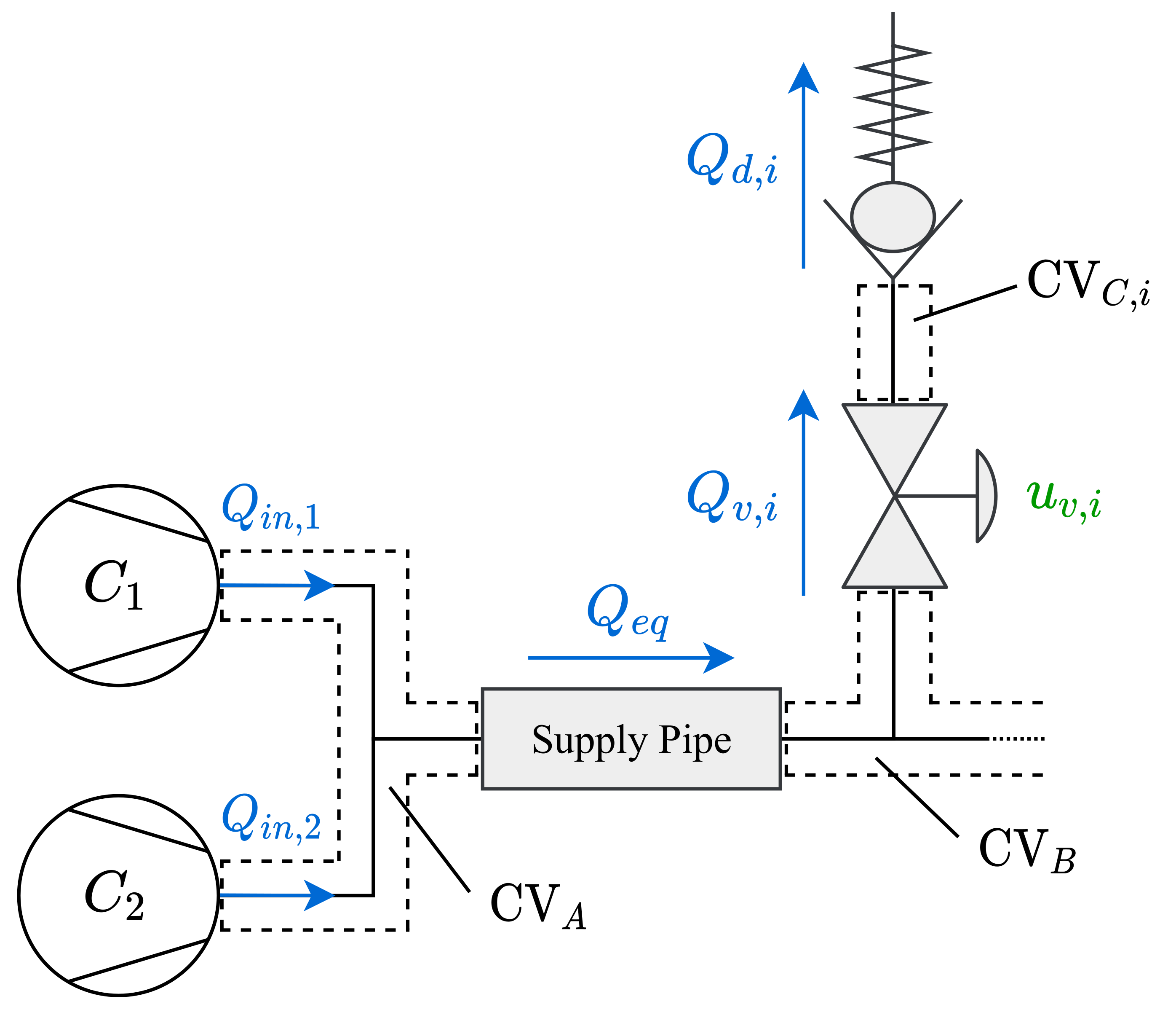
The airflow distribution network can be modelled from Bernoulli’s equation, with the pipe pressure losses approximated by the Darcy-Weisbach equation and static pressure losses from components [28,55]. The flow elements: valves and air diffusers, are modelled based on known physical relations and by fitting polynomials to manufacturers’ data. A diagram of the relevant elements in the airflow distribution network is shown in Figure 5.
Note that the diffuser flow is unidirectional to assure no wastewater flows into the pipes, hence, it is illustrated as a check valve in Figure 5. The signals introduced in Figure 5 and the symbolic notation used in this section is summarized in Table 3.
3.1. Mass Balances
The airflow distribution network can be modelled using the principle of mass conservation. First, we define the system state vector, , which represents the mass of air in the six control volumes:
where and represent the mass of air in and , respectively. The states are the mass of air in control volume , which is the volume between the valve and diffusers in each tank. Applying the equations of conservation yields the state equations in (2).
The simple form of Bernoulli’s equation is valid for incompressible flows i.e., gases moving at low Mach number (<0.3 [56]). The Mach number in the supply pipe is estimated to , indicating that the compressibility of the gas can be neglected, since the internal forces induced by the fluid motion are not sufficiently large to cause a significant change in the fluid density [56]. Therefore, the densities and pressure changes in the system can be modelled based on the ideal gas law:
where denotes the mass in the control volumes, and R, M and T denote the universal gas constant, molar mass, and temperature of air, respectively. Estimates of the volumes , and are made based on construction schematics of the case plant.
3.2. Pipe Friction Losses
To account for pressure losses in the main supply pipe due to friction between the air and the pipe surface, friction losses are implemented in the airflow model. Friction losses in the supply pipe can be calculated based on the Darcy-Weisbach equation, applying the methodology described in [19,51]. The Darcy-Weisbach equation expresses the dynamic pressure difference from to , , due to friction in the supply pipe as:
where is the fluid density, D is the pipe diameter, L is the pipe length and is the area-averaged velocity through the supply pipe. Lastly, is the friction factor that is solved directly using the Swamee and Jain approximation in Equation (5).
In which is the absolute roughness factor of the inner pipe and Re is the Reynolds number. The Reynolds number, calculated by Equation (6), is updated with respect to the average flow velocity, .
In Equation (6), is the dynamic viscosity.
3.3. Diffuser Model
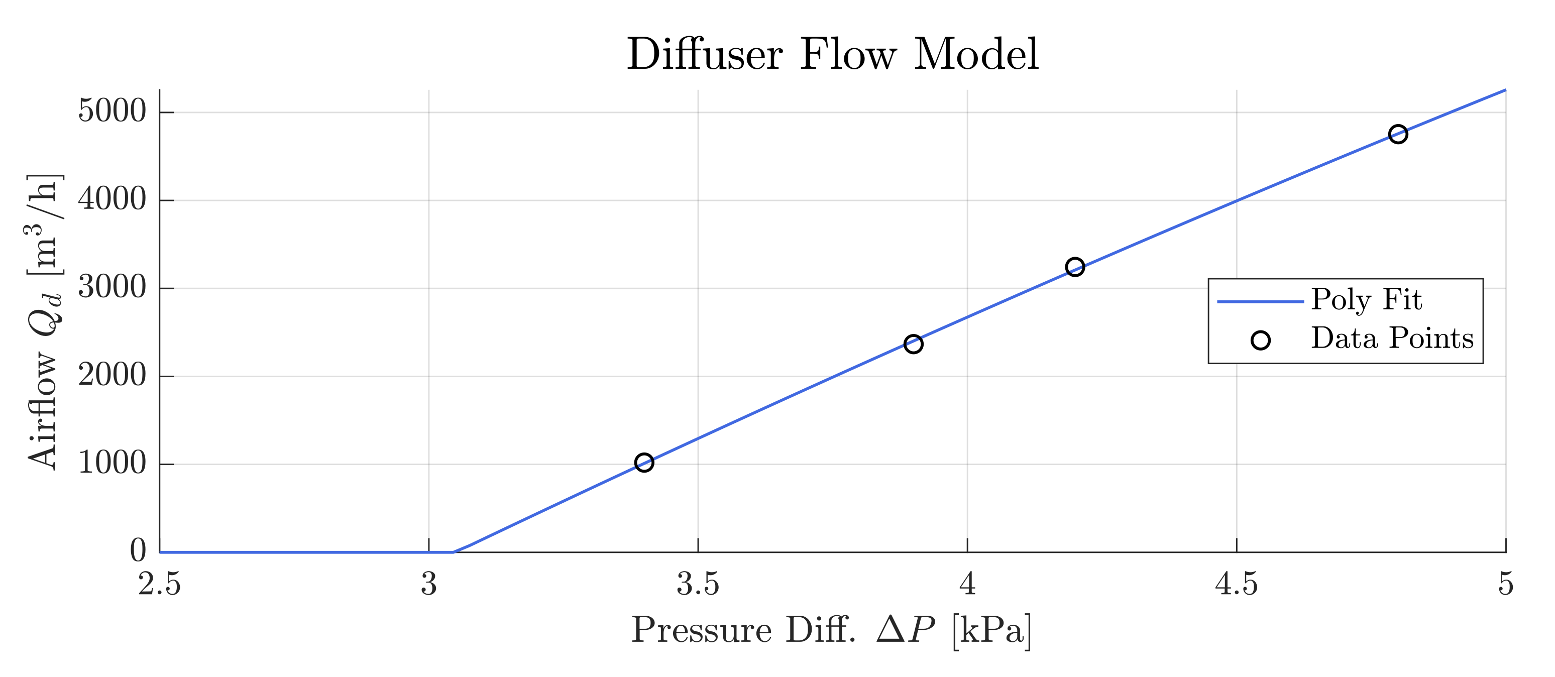
The diffuser membranes ensures that air can flow into the tank without water flowing back into the air supply system, resulting in a pressure drop caused by frictional forces of the diffuser membranes. The relation between pressure drops and airflow across the diffusers was estimated by fitting a polynomial to data provided by the case plant operators. The resulting model is shown in Figure 6. The pressure drop at the diffusers can be approximated by summation of static pressure losses of main components; manifold, diffuser piping, membranes, and hydro-static pressure [28]. Thus, the pressure difference is defined as , where is the hydro-static pressure and is the equivalent pressure losses in flow elements. As , changes in had minor effects on the overall simulation result, hence, it was considered a tuning parameter.
The airflow through the diffusers can therefore be described by the polynomial fit in Equation (7).
In which a, b and c are the fitted model parameters. Note the dead-zone from 0 to 3.05 kPa where the airflow is 0 due to the unidirectional flow through the diffusers. Imperfections in the pipeline, such as cracks and leaks, result in a leakage flow. We define a leakage flow constant to describe the gradual convergence towards equilibrium pressure (atmospheric) when the air supply is turned off. Laminar flow can be assumed for leakage flows [57], and the diffuser flow is hereby computed by Equation (8).
where is a leakage constant, and is regarded as a tuning constant, and is the atmospheric pressure. Note the leakage term only becomes relevant when the corresponding diffuser airflow approaches zero.
3.4. Valve and Flow Sensor Models
For a given pressure, the nature of airflow is dependent on the dimensions and geometry of the opening. For well-defined, purpose provided openings such as valves, airflow is usually assumed to be turbulent [58,59] and is often approximated by the orifice Equation (9). The following assumptions are made to apply the method [59]:
- Assumption 1
- The gas is an ideal gas and the flow through the orifice is steady.
- Assumption 2
- Flow through the orifice is an adiabatic process; there is no heat exchange with the surroundings.
- Assumption 3
- The upstream flow velocity (inlet) is much smaller than the downstream flow velocity.
- Assumption 4
- The discharge coefficient, , is constant.
The flow through the valves is measured by flow sensors, as indicated in Figure 3. The flow sensors have a relatively slow transient response, and their dynamic is therefore included in the model. The sensor dynamics are approximated by a first-order dynamic , with a time constant which was estimated to 55 s. Adding the sensor dynamics to the model we obtain the following model for the flow:
3.5. Combined Model
The models obtained in Section 3.1, Section 3.2, Section 3.3 and Section 3.4 are combined and referred to as the airflow distribution network. Figure 7 shows a flowchart of the algorithm used to simulate the model.
The inputs to the model are: the pressure measurement in , , the states of all valves, , and the air temperature measured at the inlet of the compressors, T. The output of the model is the airflow through all control valves, . The algorithm is executed with a sample time . Steps 1–5 presented in Figure 7 are elaborated below:
3.6. Parameter Identification
The structure and parameterization of the model derived up until now was based on well-known physical principles. Some model elements were taken from manufacturer data sources, others based on geometrical dimensions by applying well known formulae. The model parameters have been listed in Table A1 in the Appendix A. The only remaining unknowns are the discharge coefficients, , which could be approximated experimentally or found in manufacturer data. However, given that the objective of the model is predicting the airflow distribution accurately, the parameters are instead computationally identified for each branch to optimize model prediction. The benefit of this method is that any uncertainty introduced in the different flow elements: diffusers, manifold, pipe friction etc. can be compensated for by adjusting the discharge coefficient accordingly in the respective branches.
The airflow model algorithm visualized in Figure 7 is used to perform an open-loop simulation with the given input signals being real case plant data. The optimal values were estimated using the MATLAB function fminsearch, which applies the Nelder-Mead (NM) “simplex” search algorithm [60,61]. The methodology is further discussed in [28]. The cost function subject to minimization was defined as the sum of squared errors (SSE) for all data points, N, for each branch, i, as described by Equation (11).
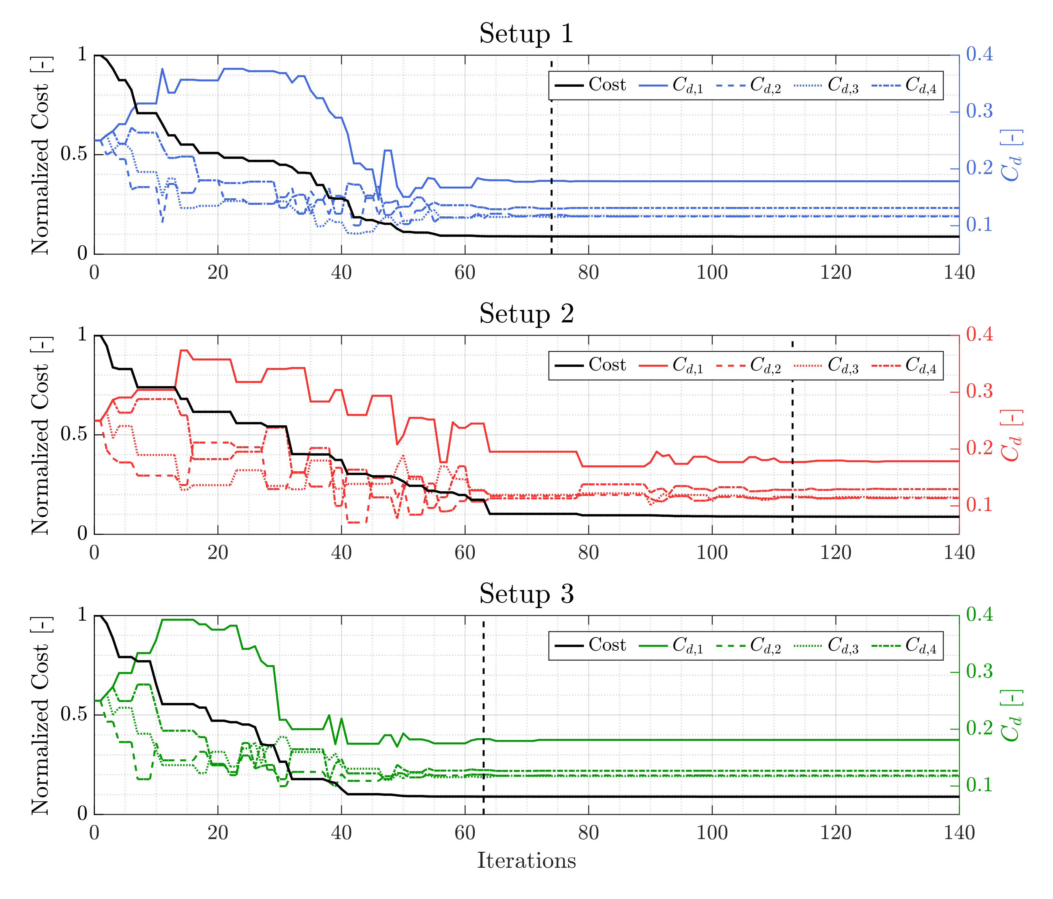
where is the k’th airflow measurement to the i’th tank. is the model estimate of the airflow. A subset of 16 h in the nine day dataset was used for identification. As it is known from the work [62], the NM method is sensitive to initial simplex points and values of NM coefficients, i.e., reflection , expansion , contraction and simplex size . Therefore, we have applied the NM method with different coefficients proposed in [63,64], the coefficients () and the resulting cost functions have been shown in Table 4. The iterative estimation of the discharge coefficients is shown in Figure 8, where it can be seen that the cost function converges to a specific minimum.
The analysis shows that the used approach is not sensitive to variations in the four aforementioned NM coefficients, as the final cost and the obtained values for all three setups lies within a close margin. We can observe that setup 3 has the most efficient algorithm behaviour, requiring least iterations to obtain the desired cost.
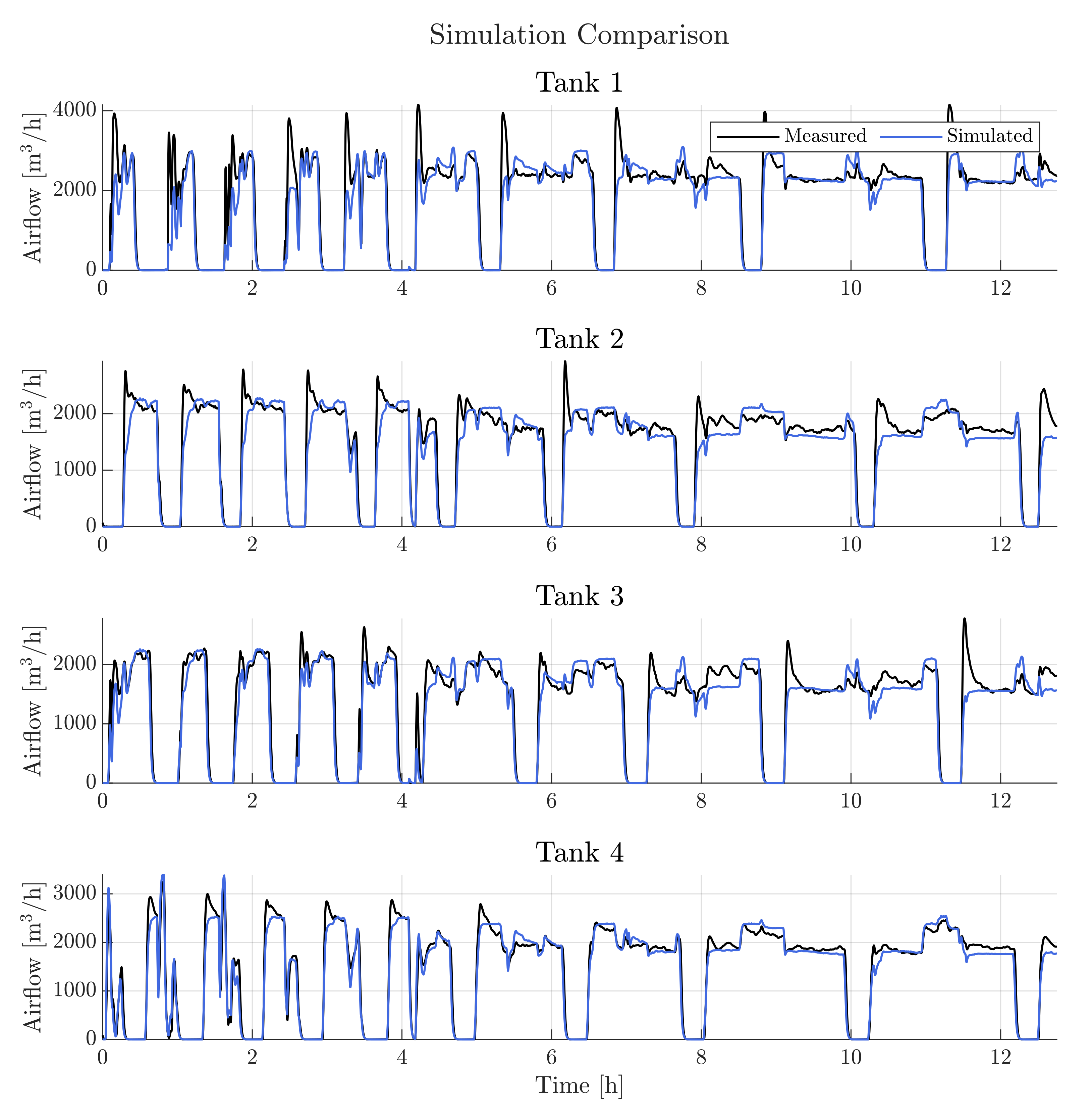
A goodness-of-fit (GOF) based on the normalized root mean square error (NRMSE) was used as a metric for model performance (higher is better). The metric is calculated for each distribution line and listed in Table 5.
In Figure 9, a comparison of the measured and simulated airflow is shown. The proposed model is able to reproduce measurements outside the identification subset and considered to be a sufficient model for designing and testing control algorithms in later sections.
The airflow model is obtained from first principles, and is suited to model any other airflow distribution network, as long as the constant parameters related to the case plant layout are known (i.e., pipe lengths, diameters, tank volumes, discharge coefficients, etc.). However, given that the parameters are fitted to experimental data and identified for each branch to optimize model prediction, the model now becomes an empirical model. Nevertheless, the presented method remains applicable as long as the discharge coefficients are considered adjustable parameters and plant data is available for model fitting.
3.7. System Curves
This section introduces a steady-state pressure-flow relation of the airflow system. The pressure-flow relation is essential when controlling the compressors. Depending on the pipes, the manifolds, the valves, or the hydro-static pressure, the terminal impedance that the compressors have to overcome, i.e., the system curve, changes [65,66]. As a result, the action of regulating the valves change the system characteristics, thus, appropriate control of the compressors is essential to maintain optimal efficiency operation [65]. Generally, a system curve is described by Equation (12) [65].
where is the static pressure the compressor system needs to lift, and is a pressure loss coefficient of the flow rate, Q. Due to the variable system characteristics resulting from the flow regulating valves, and should be considered as functions of the valve states, , or more specifically by the sum of open valves, , given in Equation (13).
Assuming the coefficients ( and ) are known for a particular system state, then the possible combinations of pressure and airflow must exist on that system curve [65]. This property is useful both for compressor scheduling and pressure control, as will be discussed in the following sections.
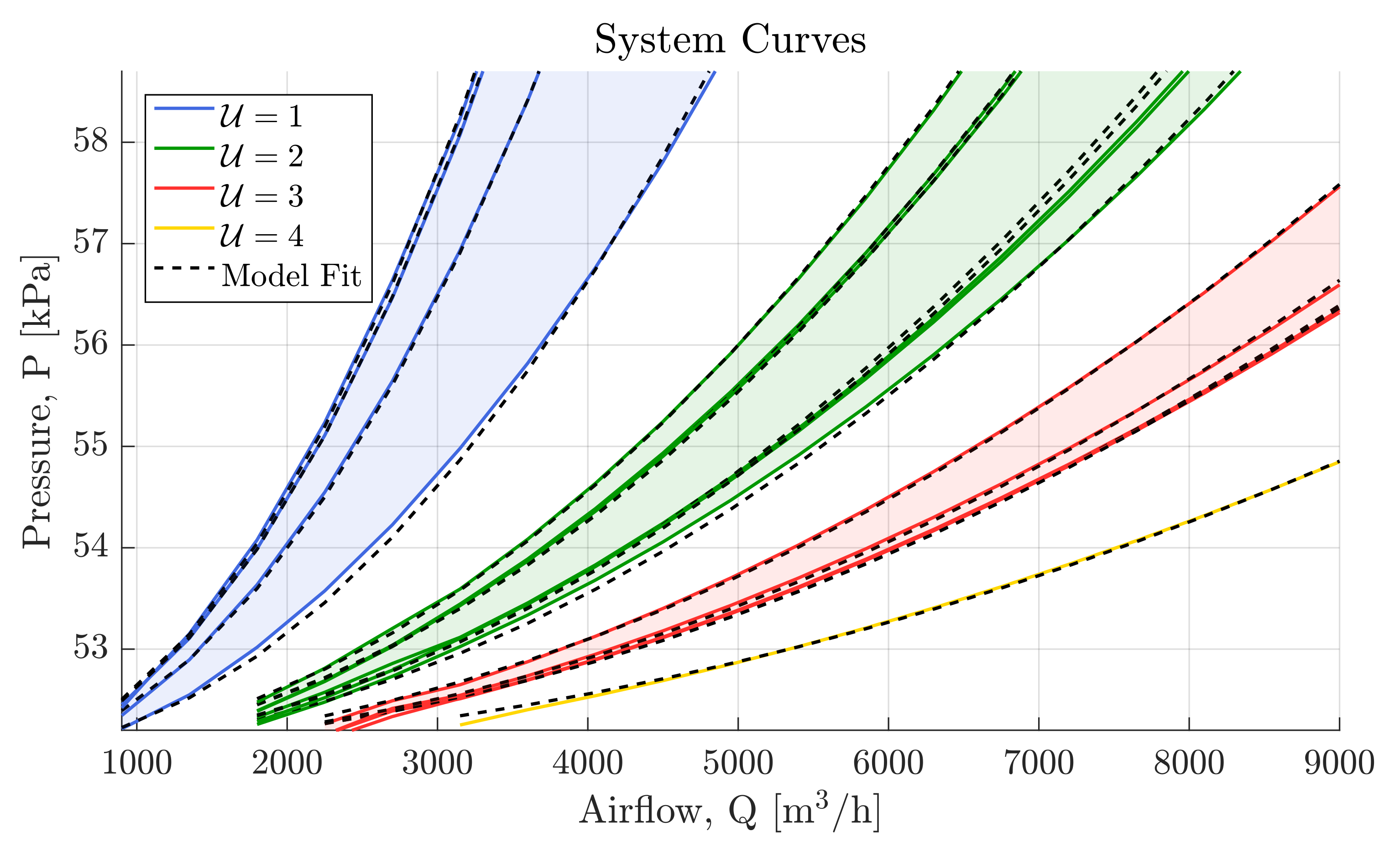
The procedure of estimating the pressure coefficients is performed on the simulation model of the airflow system. With four aeration tanks, the number of different valve combinations increase by the fourth power i.e., , where x denote the number of valve states (two for on/off). A staircase airflow signal is used to excite the system, and the steady-state pressure is logged. This process is then repeated times, corresponding to the number of valves opening combinations. All pressure curve combinations with on/off controlled valves are displayed in Figure 10. The individual curves are sorted by color with respect to the sum of open valves, .
As the valves in practice could operate at various intermediate states, the number of combinations increase significantly. In this work, combinations with four opening states are simulated; fully closed, 13bevelledtrue open, 23bevelledtrue open and fully open. The estimation procedure of the pressure coefficients was done recursively, where both and were estimated in the first iteration. Then was averaged over all valve combinations and locked in the subsequent estimation. Thus, simplifying the parameterization of operating points to alone. Subsequently, the pressure coefficient was allocated to a look-up-table (LUT) with cells for the various valve combinations. The resulting models have been illustrated in Figure 10. For values between grid points, the output is interpolated from neighbouring points, which means true system curves are not guaranteed. As a result, control must be achieved in combination with a feedback controller, which also compensates for disturbances.
4. Pressure Control
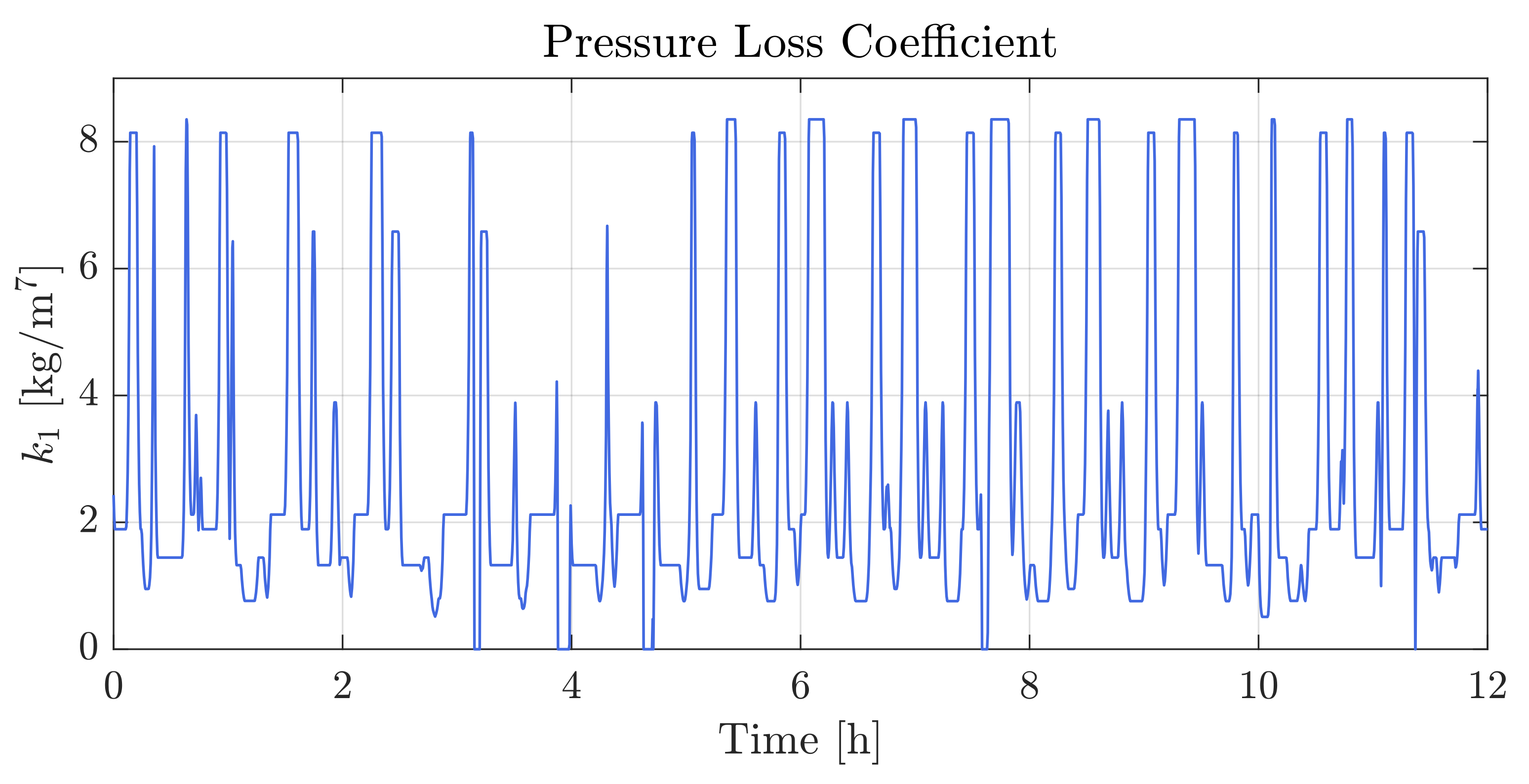
In Section 3.7 the steady-state pressure-flow relation was introduced, and as shown in Figure 10, the system characteristics change significantly with respect to the sum of open valves, . As a result, stabilizing the system is challenging. However, the information contained in the coefficients can be utilized in a control scheme as presented in this section. The system curve was expressed by Equation (12) in terms of the pressure coefficients, and , and it was made clear that different combinations of valve states could alter their values. Using case plant data for the valve openings , the system flow can be simulated using the algorithm described in Section 3.5 and visualized in Figure 7. This simulation data can be used to estimate in Equation (12). A time series of the estimated coefficient is shown in Figure 11, which clearly illustrates the changing system characteristics.
One way to deal with the changing system characteristics is to exploit the process information stored in the pressure coefficient look-up table. This methodology is often used to compensate for known disturbances (changes in variables) before the process is significantly upset [67,68,69].
Three control schemes are evaluated in this section: a benchmark PID controller (benchmark PID), a LUT-feedforward controller (LUT-FF) and a LUT-feedforward-feedback controller (LUT-FF-FB). To evaluate the control schemes, a simulation comparison is evaluated using an artificial pressure reference, generated based on the number of open valves. The simulation is carried out using the airflow distribution model described in Section 3. As the flow regulating valves in practice have long opening times (>140 s rise-time) compared to the compressor dynamics (<15 s rise-time), the compressor dynamics are assumed to be negligible overall.
4.1. Benchmark PID Controller (Benchmark PID)
A traditional PID controller is designed functioning as a benchmark solution for evaluation of the proposed controllers. As the system in this case is heavily coupled and does not have a single operating point that could be used as an equilibrium for linearization, the benchmark PID control parameters are determined using Ziegler–Nichols (ZN) tuning method. The performance of the tuned controller is shown in Figure 12.
When implementing the controller, the control input is saturated between 1200 and 11,000 m/h, reflecting the physical limitations of the compressor system. To tackle the problems emerging from the limits in compressor flow capacity, anti-windup is implemented to avoid operating in infeasible regions. Additionally, the input is considered as a single signal, although two compressors supply the flow in practice. A method for sharing the flow load between compressors will be discussed later.
4.2. LUT-Feedforward Controller (LUT-FF)
The nonlinearity introduced by the varying pressure coefficient, , can be corrected for by implementing a feedforward control law. Assuming the present valve states are known, the pressure coefficient can be found in the LUT previously described. Subsequently, any combination of pressure reference and airflow exists on the system curve, meaning the feedforward control input can be computed by inverting Equation (12) resulting in Equation (14).
In practice, the feedforward term alone is an open-loop controller. Hence, disturbances introduced by the difference between estimated pressure coefficients () and the real system are not corrected when applying feedforward control. However, it is included in the comparison to illustrate the effect of the feedforward term.
4.3. LUT-Feedforward-Feedback Controller (LUT-FF-FB)
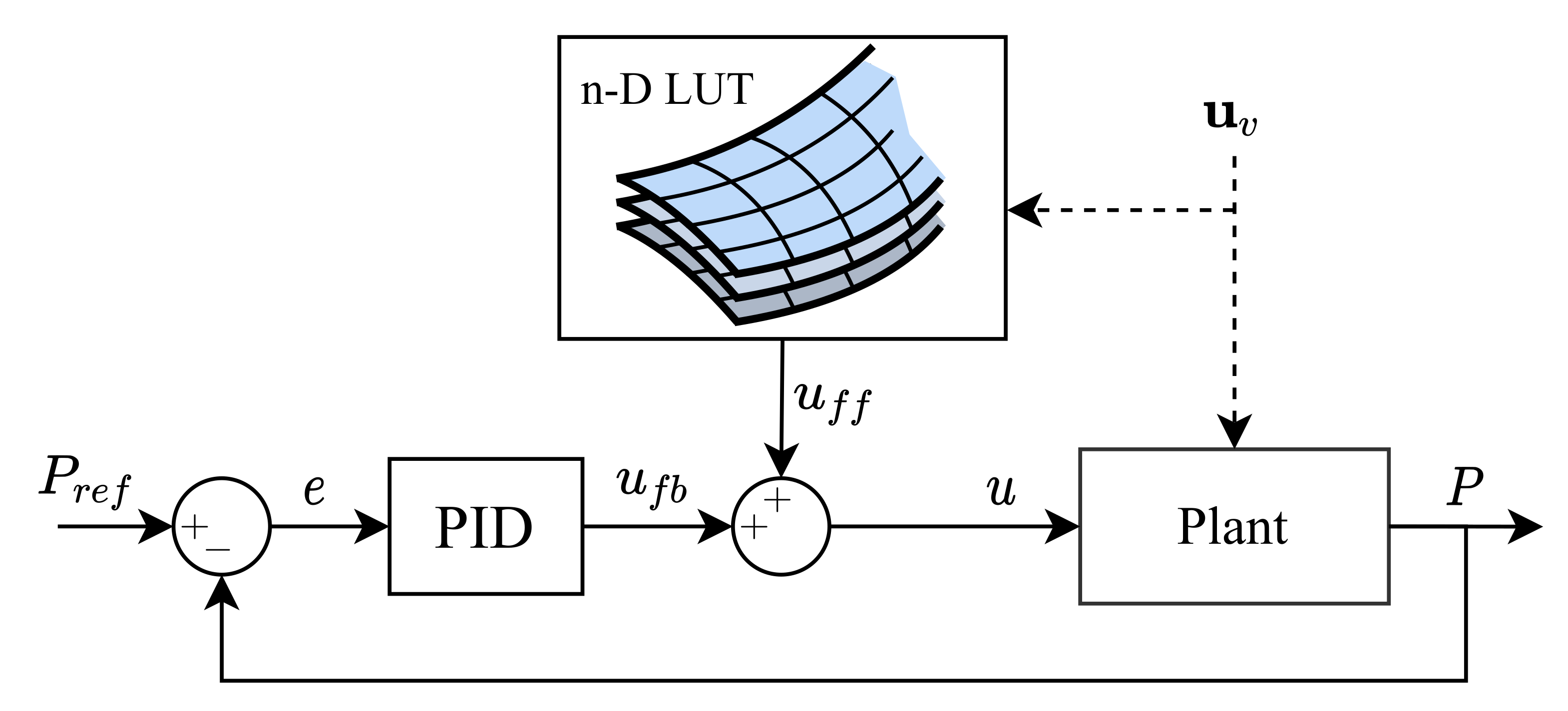
Feedforward control on its own may lead to unsatisfactory behaviour, especially if the estimated system curves are inaccurate. A method to improve regulatory control is to combine the feedforward term with a feedback controller [67]. In this scheme, the LUT-FF enables early compensation of a measured disturbance before it can seriously affect the process. An ideal feedforward controller, based on direct inversion of the system, is often not physically realizable [67], and the feedback controller is hence used to compensate for errors caused by the non-ideal feedforward controller (due to uncertainties in the estimated operating points). The structure of the combined PID and feedforward controller (LUT-FF-FB) is shown in Figure 13.
The tuning procedure selected for the PID feedback controller for the LUT-FF-FB is the ZN approach, and its performance is compared with the benchmark PID solution and the LUT-FF in Figure 12.
Figure 12 shows a comparison of the three proposed controllers. Compared to the benchmark PID and the LUT-FF-FB, the LUT-FF shows poor reference tracking performance, especially during transient periods, when characteristics of the system change. However, when observing the control input generated by the LUT-FF, this actuation signal is moderate compared to the two other controllers. Both the Benchmark PID and the LUT-FF-FB track the pressure reference relatively accurately, however, the Benchmark PID has to make considerably larger input corrections, which can be seen in Figure 12b. As an example, the control input oscillates up to 2000 [m/h] (peak to peak) at the time interval 0.4–0.5 h. This behaviour is not desirable from a physical point of view, as it requires sudden acceleration and deceleration of the compressors, resulting in an increase in power consumption [43]. The tuning procedure of the benchmark PID becomes a trade-off of fast dynamic response against overshoots and oscillations. On the other hand, the main goal of the feedback controller in the LUT-FF-FB is to compensate for minor irregularities or disturbances, allowing it to be designed less aggressive. In conclusion, the LUT-FF-FB has the best performance, as the control input is fairly moderate and improves pressure reference tracking during time-varying operating conditions.
5. Compressor Scheduling
The aim of the compressor scheduling algorithm is to improve energy efficiency of the compressors. This goal is achieved by first obtaining static power models of the case plant compressors and subsequently implementing an algorithm that adapts to the changing system states.
5.1. Static Power Model
To find the optimal scheduling strategy, a model of the compressors will be developed in this section. The model is a static map describing the relationship between electrical power, pressure and airflow, denoted as . The following assumptions are made to justify the deduced model:
- Assumption 1
- The transient dynamics of the compressors are assumed fast enough to be neglected, meaning that static models are adequate to describe the system.
- Assumption 2
- The efficiency of the motor and motor driver is constant. This implies that the system efficiency, , can be defined as the ratio of hydraulic power to electric power [65].
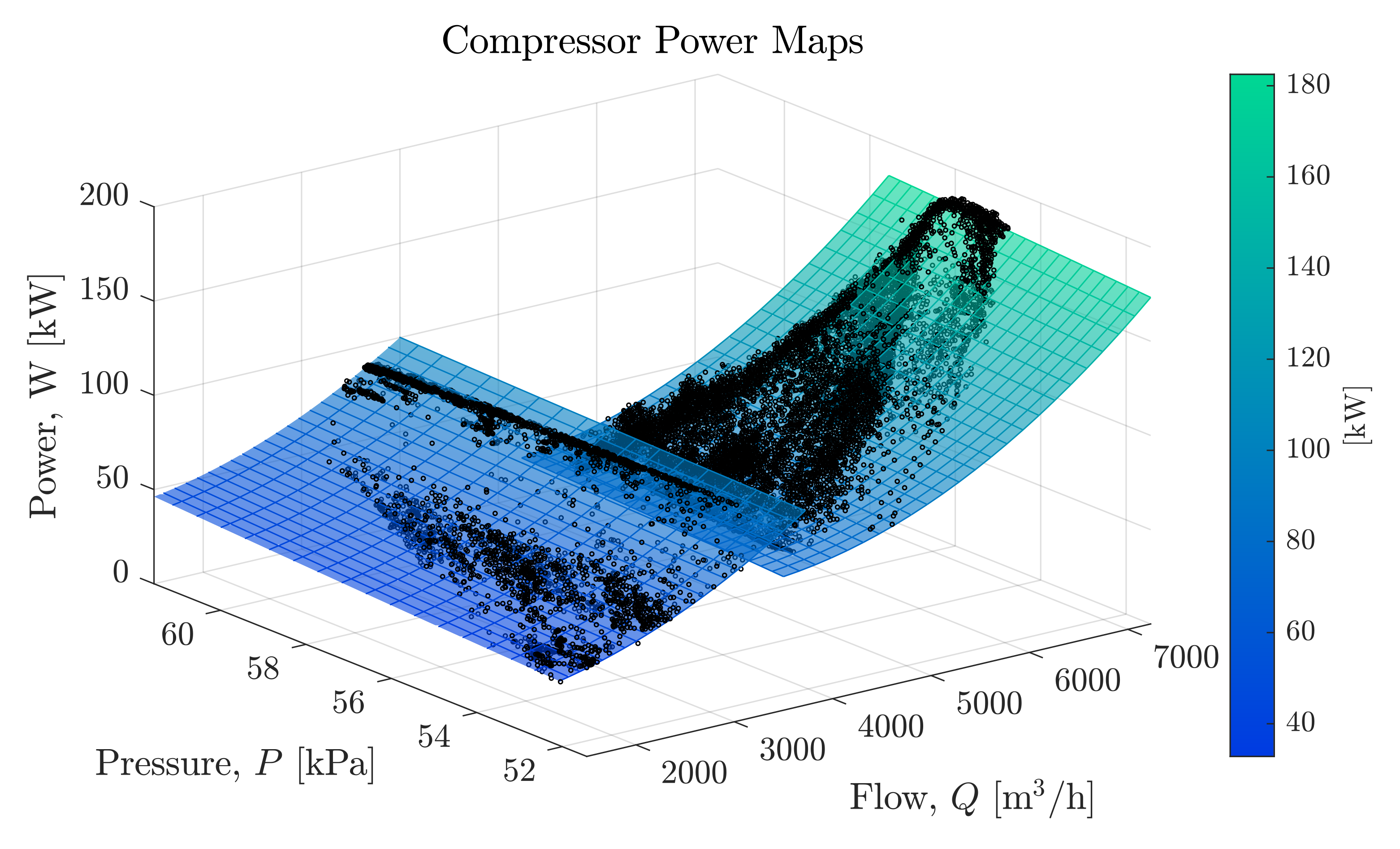
Models for compressor performance have been proposed in [70,71,72], however, no general structure is suggested. The 2nd-order polynomial structure from [72] is chosen due to its fitness to the data, hence, the compressor power map is defined by Equation (15).
where P and Q denote gauge pressure and airflow, and are constant model parameters. Note that the model structure does not explicitly describe the relationship with compressor speed, which also affects power consumption [70,73]. However, it indirectly describes it, as only one possible compressor speed for a given pressure and flow rate exists, hence why speed is not directly present in Equation (15). This means that is well-defined with only 2 degrees of freedom between W, P and Q. The model parameters reflect the specific compressor characteristics, and they could be identified through experimentation by manipulating system head and airflow [65,70]. However, in an industrial plant where operation down-time results in pollution of nitrogen to the surrounding environment, an estimation procedure based on daily operation data was necessary. Both power consumption (W), airflow (Q) and pressure (P) were included in the case plant data-set making this procedure possible. With a slowly changing system (aeration cycles of +20 min), several operating points could be extracted when the system had reached an equilibrium, i.e., where pressure and airflow gradients were and . The data points and resulting fitted power maps are shown in Figure 14.
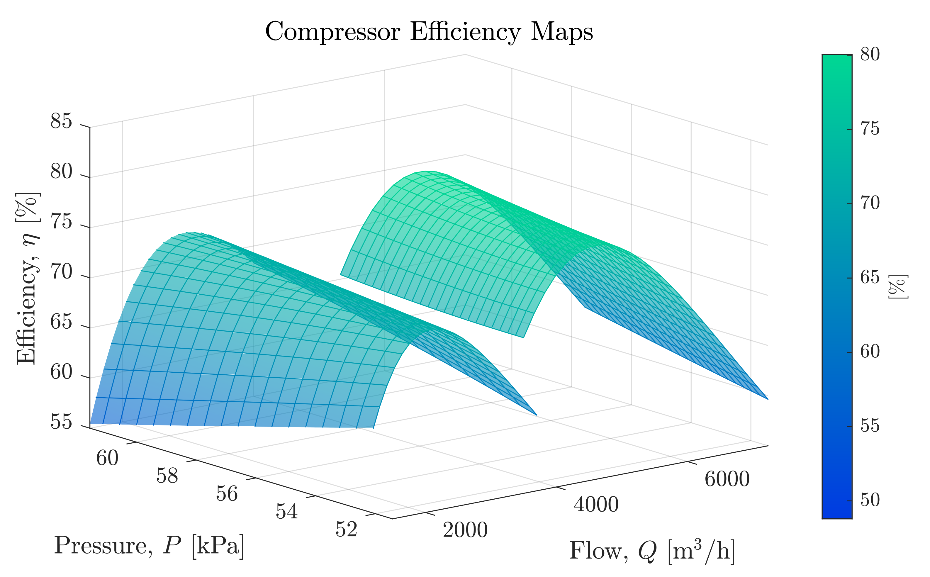
The power maps shown in Figure 14 can be used to derive the efficiency maps of the compressors. The compressor efficiency, , is defined as the ratio of hydraulic power to electric power [23,73]. The electric power is measured at the motor driver, meaning it includes losses in the entire drive-train. This yields Equation (16), which maps the compressor efficiency.
Then the compressor efficiency can be computed explicitly for a specific pressure and airflow. The resulting compressor efficiency maps are shown in Figure 15.
The power maps are based on a general structure without considering the physical principles of the system, hence, the feasible window of operation of the compressors are defined from the domain of the regression model in both flow and pressure [53]. Practically, each compressor can only supply flow rates within a specific lower and upper boundary according to its size. The lower and upper boundaries are considered in the derivation and are denoted by the subscripts and .
5.2. Compressor Load Sharing
The characteristics of any number of parallel-connected compressors, , can be computed by summarizing flow and power for the individual units [65,72,73]. Thus, for any number of compressors the air supply characteristics are defined by Equations (17) and (18).
where Q, P, W and are the flow, pressure, power, and efficiency in the combined air supply system. and is the lower and upper flow limits that compressor j can deliver while and is the lower and upper pressure limits that the system can reach, respectively. By taking advantage of the characteristics of the compressor units, i.e., the different power and efficiency maps, the energy consumption of a network of compressors may be improved [43,53]. Different strategies have been applied to share the load of multiple compressors, refer to [53,74]. Ref. [74] argues that compressors with identical compressor maps, may equally split the load or operate at the same surge margin. Additionally, it was reported that for two compressors with very different efficiency characteristics, the larger (or more efficient) unit should carry the base load, while the smaller (or less efficient) unit is responsible for load fluctuations. Finally, another option is to distribute the load by using an optimization routine like proposed in [53,75]. The compressors installed at the case plant considered in this study exhibit similar efficiency characteristics, hence, the equal load split method is applied in this work. This method is advantageous in the proposed scheduling algorithm, as only the desired load percentage is to be optimized for a given compressor configuration [53]. Thus, for any number of operational compressors, the airflow delivered by each unit, j, is defined as by Equation (19).
where is the percentage loading for all compressors going from (idle) to (fully loaded), Q is the total air flow required, is the lower flow limits for all compressors and is the upper flow flow limits. is a binary decision vector denoting whether the respective compressor is active (1) or inactive (0):
The investigated air supply system consists of two parallel-connected compressors, meaning three pump combinations exists (excluding the default case with both being inactive). Generally, a pump system consists of possible configurations.
5.3. Scheduling Algorithm
Assuming the pressure coefficients, and , are known for a particular system state, then the possible combinations of pressure and flow rate must exist on the system curve, as per Equation (12). Thus, the system has only one degree of freedom between P and Q, and by extension one degree of freedom for . This property can be used to select a combination of airflow and pressure reference maximizing the compressor efficiency. Finally, scheduling between compressors can be performed by selecting the combination with the highest efficiency.
Applying the LUT introduced in Section 3.7 and given as the pressure coefficients in Equation (12) at any combination of valve states, allows an estimate of the system curve to be made. Once the flow and pressure relationship is locked, both power and efficiency characteristics are computed for all compressor combinations using the defined formulae; (17) and (18).
The goal of the scheduling algorithm is to obtain the operating point and select the respective compressor that maximizes the efficiency of the air supply system. However, the solution should also be subject to constraints specific to the case plant. In this work two main constraints are considered:
- Constraint 1
- The solution should be within the flow and pressure ranges defined in Equation (17). This constraint ensures that the air supply system never exceeds the physical limitations in pressure drop across the diffusers or approaches the limits of operation (surge/stall) for the compressors.
- Constraint 2
- To facilitate biochemical treatment a minimum airflow supply for each reactor is required (), therefore, the air supply is subject to:
The proposed algorithm evaluates the compressor efficiency in various operating points and determines the maximum feasible efficiency subject to the above constraints. It follows the procedure presented in Algorithm 1:
| Algorithm 1: Compressor scheduling algorithm pseudo code. |
 |
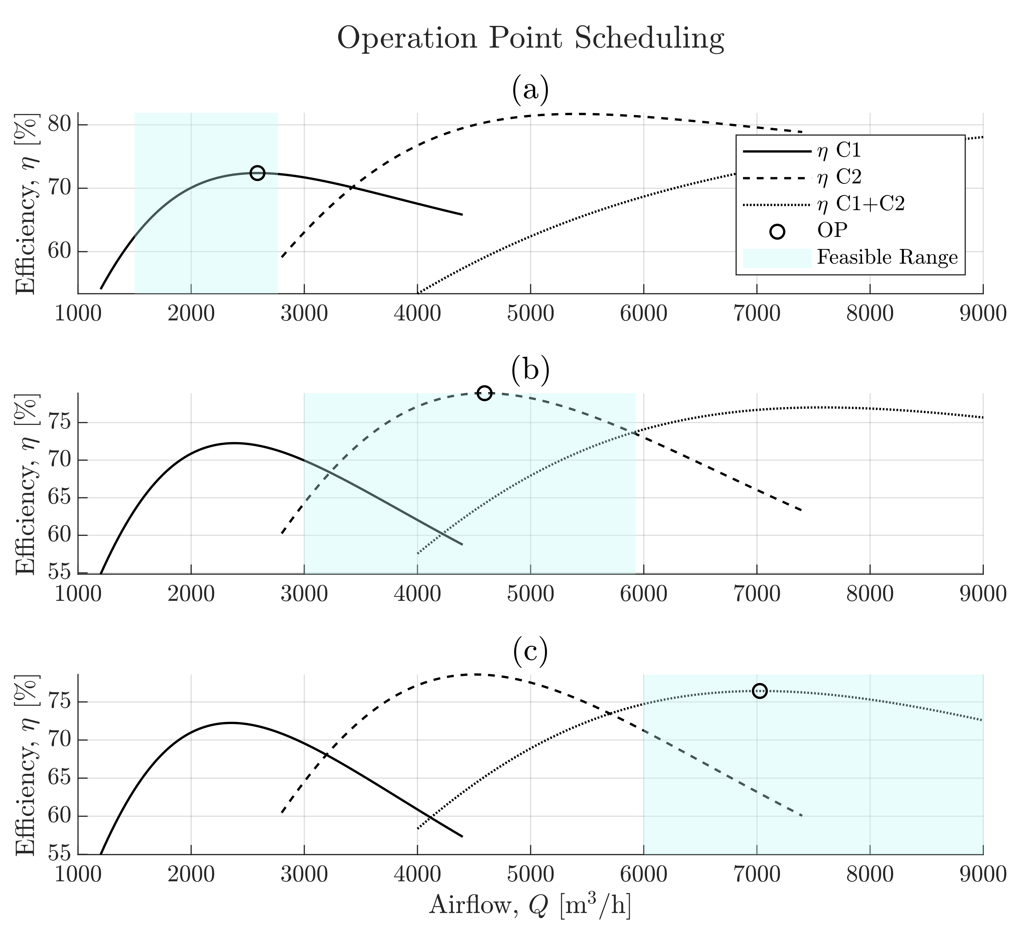
The results for different operating points have been shown in Figure 16. The blue region marks the feasible solution range with regards to the pressure constraint.
The proposed method maximizes the efficiency of the compressor system in configuration (a), (b) and (c), while considering the system specific constraints.
6. Results
Reducing the energy consumption in the aeration system is the main goal of this work. The most straight forward way of achieving this is by not aerating, however, this would severely compromise the performance of the nitrification/denitrification processes. Hence, rather than comparing the actual energy consumption explicitly, the energy efficiency of the compressors is a more suitable measure for examining the scheduling performance. Using the energy efficiency and the number of restarts per day as evaluation criterion, the current and the new proposed compressor scheduling are compared in this section. The justification for using restarts per day is that they are directly related to compressor wear and tear and increased energy consumption [76,77,78,79].
The scheduling algorithm introduced in Section 5.3 was implemented on the airflow network model and simulated in parallel with the 9-day data-set from the real plant. The power consumption and efficiency models introduced in Section 5 were derived based on data from daily operation and reflects the performance of the real system and simulated plant alike. Thus, the efficiency of the compressors is directly comparable between the simulated and real system.
Intervals from the simulation have been highlighted in Figure 17 and Figure 18 to comment on the performance of the proposed scheduling algorithm.
On the case plant the compressor control consists of two rules Control Rule 1 and Control Rule 2. The compressor installations were based on the flow demand, meaning the small compressor (C1) and the large compressor (C2) were selected to have the best operating point (BEP) close to the demanded flow when:
- Control Rule 1
- one valve is completely open → start C1
- Control Rule 2
- two valves are completely open → start C2
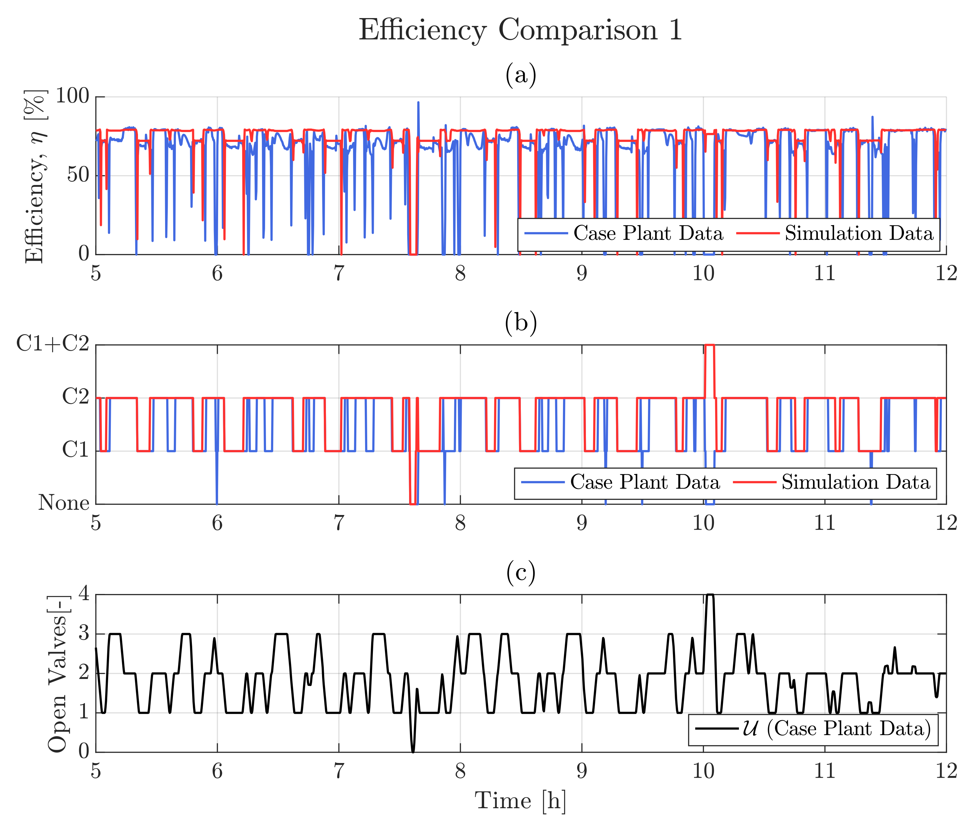
As a result, the efficiency of the case plant matches the maximum efficiency of the proposed scheduling algorithm when 1–2 valves are completely open, which can be seen in Figure 17. Furthermore, Figure 17 shows a significant improvement since the proposed scheduling algorithm ensures fewer start-ups despite switching between 1 and two completely open valves. In the case plant, the compressors start and stop according to Control Rule 1 and Control Rule 2 in addition to some on-time and off-time constraints to limit switching frequency of the compressors. The proposed scheduling algorithm reduces switching by alternating between compressors depending on the case plant pressure curves and the pressure constraints set for the maximization of . This is made clear in the interval 6–8 [h] in Figure 17.
Depending on which pair of valves are open, the system pressure curves can change significantly as illustrated previously in Figure 10. Consequently, the rule-based compressor control, (Control Rule 1 and Control Rule 2), does not always ensure operation close to the BEP. This is evident from Figure 18, where the efficiency drops as a result of system curve changes between valves states (e.g., when 2–3 valves are open). It should also be noted that the efficiency when 3–4 valves are open drops significantly in the case plant, which is due to the compressors not operating in parallel.
Based on the entire data-set, the efficiency with different number of open valves have been averaged. The metrics used for comparison are listed in Table 6.
Referring to Table 6 the proposed scheduling algorithm improves efficiency in all cases and reduces the amount of compressor restarts. In agreement with our hypothesis, the improvement in the 2-valve scenario is much smaller in relation to the other operating points. The reason for this is that the case plant is designed to be most efficient when two valves are open. A similar statement could be said for the 1-valve scenario; however, we presume the efficiency improvement is a result of having very different system curves depending on which tank is active, leading to operation at flow rates away from the BEP. In conclusion, the simulation results shows that the proposed scheduling algorithm is advantageous to the current rule-based control employed in the case plant.
7. Discussion
The purpose of this work is to improve the aeration energy efficiency of the case plant ASP. In this work, the dynamic pressure control and compressor scheduling is examined with the focus on reducing energy consumption without compromising effluent quality. Contrary to other studies, this work is focused on the characteristics and design of the parallel compressor setup and proposes an algorithm to choose the best configuration for any possible system state.
To address the problem of improving the energy efficiency of the aeration process, first an airflow model is obtained. The airflow distribution is modelled by a well-established method using mass balances, Bernoulli’s principle, and the Darcy–Weisbach friction equation, similar to the approach in [19]. This approach is used since a detailed airflow model provides insights into the system dynamics and enables optimization of the process performance and efficiency [55]. Additionally, the detailed air distribution model provides the best basis for DO modelling, as it is evident that all aeration tanks are not provided with equal airflow [19,55]. Two main approximations of parameters are made to fit the model to actual plant data:
- Flow sensor dynamics are approximated assuming a first-order filter, resulting in the model being fitted to the damped sensor measurements rather than the actual flows. This is however a necessity as there is no other option for validating the airflow distribution model without changing the system setup and implementing another sensor. Should another, faster sensor (like a pressure transmitter) be implemented, the sensor dynamics should still be modelled despite the faster dynamics, as these dynamics most likely would contribute to the over-all system dynamics.
- Valve discharge coefficients which are estimated using a numerical method minimizing a cost function. By using this approach, the estimated parameters are not identified to fit the actual discharge coefficients of the valves alone, but instead an estimate of a general “loss coefficient” for the entire system, compensating for and eliminating many of the uncertainties introduced when modelling other flow elements.
With these two approximations, both eliminating minor modelling errors and uncertainties, the airflow distribution model estimates the actual airflow over each valve with only small deviations and an overall fit percentage of approximately 68%.
Through simulations, the airflow model is subsequently used to produce the system curves for 175 different valve combinations, making it possible to simplify the system pressure curves as a second order polynomial model. The system curve models are determined, and the static pressure coefficient and pressure loss coefficient is then arranged in a look-up table (LUT) which lays the foundation for both the LUT-FF-FB pressure controller and the new proposed scheduling algorithm.
The dynamic pressure control is designed similar to the approach used in [68], which is often used in automotive applications, and involves feedback-feedforward control strategy. The combined feedback-feedforward controller (LUT-FF-FB) overcomes the operating-point dependent nonlinearities and shows better tracking performance than the benchmark PID. The static LUT-FF is used to generate the feedforward signal,
The scheduling algorithm is based on the system curves, from which the optimal flow rate is computed in the form of a pressure reference. Consequently, differences between the case plant data and the estimated system curve can lead to sub-optimal performance of the scheduling algorithm. This difference is compensated by the feedback term in the LUT-FF-FB algorithm. Using the energy efficiency of the compressors and average restarts per day as performance measures, the rule-based scheduling algorithm implemented on the case plant and the proposed scheduling algorithm are compared. Since up to 75% of the total electricity consumption for a WWTP is related to the aeration process, even a small increase in energy efficiency can affect the operational cost and environmental impact of the WWTP significantly. Additionally, the wear and tear of the compressors affects the lifetime and repair downtime, which is strongly related to frequent restarts of the machines [76,77,78,79].
The methods presented in this paper are limited to WWTPs and aeration systems where plant data of the valve flow, and data of the compressor flow, pressure and power consumption is available. Since the airflow model (presented in Section 3) is fitted to plant data and parameters are identified for each branch to optimize model prediction, the model now becomes an empirical model. Despite the use of empirical methods, the approach presented in this work is still applicable to any WWTP as long as the discharge coefficients are considered adjustable parameters and plant data is available for model fitting.
Despite not being modelled dynamically, the static compressor power models are obtained and considered sufficient for the purpose of designing an energy efficient scheduling algorithm. This is justified by assuming that the transient dynamics of the compressors are fast enough to be neglected. Consequently, the usefulness of the scheduling algorithm proposed in this work is limited to larger airflow systems, where the pipe network is large enough to dominate the overall system dynamics. As this is a distinctive feature for most wastewater treatment plants, the method is regarded highly applicable in the field of wastewater treatment. Furthermore, the static compressor power maps were obtained with regression analysis without considering the physical principles of the system. Consequently, the models are not of universal character as they are invalid outside the domain of the regression model in both flow and pressure [53]. This is addressed by implementing lower and upper boundaries for the flow and pressure of each compressor (see Equation (17)).
The results of this paper are considered interesting for any WWTP with the wish to reduce energy consumption and wear and tear of the compressors, solely by algorithm implementations. It is especially appealing that the energy efficiency of the compressors is increased regardless of the system state. Table 6 frames the benefits of the new proposed scheduling strategy, while Figure 17 and Figure 18 shows that the total efficiency of the system hovers close to 80% and predominantly above the current case plant efficiency. The exception being during the transient states when compressors are started or stopped and whilst the sum of open valves is exactly 2.
The benefit of this work is its generalizability and applicability for any WWTP. As the models of this work are based on first principle with numerically estimated parameters, this method can be applied to any WWTP with component data sheets and operational data available for model validation and result comparison. Furthermore, the method used in this work is conducted using data of daily operation, meaning that no downtime or additional experiments are required to follow the procedure presented in this paper.
Should the need be for experimental validation, the pressure curves, which in this study are obtained from simulations, can be experimentally determined using simple tests like described in Section 3.7. Increasing the airflow for any combination of valve states and logging the steady-state pressure will provide the necessary experimental data.
8. Conclusions
In this work, Grindsted WWTP located near Billund, Denmark is used as case plant providing the data for this simulation study, where improvements for the aeration process in the ASP is proposed. A dynamic pressure controller and optimal compressor scheduling algorithm is proposed from the energy efficiency point of view, meaning that results are compared based on efficiency of the air supply system and also the number of restarts per day for the compressors.
A first principle airflow model is developed and parameter estimation is done numerically using an optimization algorithm and case plant data. The model is subsequently validated on case plant data from daily operation and used to generate system curves representing the airflow system. Those system curves are used to generate a LUT containing pressure loss coefficients for 175 different valve configurations. This LUT is used to generate the feedforward control input to the dynamic pressure controller. Three dynamic pressure controllers are compared in this study, concluding that the LUT-FF-FB is superior to the benchmark-PID and the LUT-FF.
The generated LUT is used in the proposed scheduling algorithm as well. This scheduling algorithm determines the two compressors’ load (in percentage) based on changing system parameters in the airflow system (valves opening/closing). Comparing the new proposed scheduling algorithm with the current rule-based control shows major improvements in both energy efficiency of the compressors, and results in fewer restarts per day. The result of this study shows a clear and huge potential to improve the efficiency of any aeration process with multiple compressors supplying the airflow to aeration tanks. Note that the compressors of this case plant system are of different capacities, making this method applicable to other WWTP with multiple compressors either identical or nonidentical compressors.
From a practical point of view, the system curves should be experimentally validated before we recommend the method for extensive industrial application.
Author Contributions
Conceptualization, L.D.H., M.V. and P.D.; methodology, L.D.H., M.V. and P.D.; software, L.D.H. and M.V.; validation, L.D.H., M.V. and P.D.; formal analysis, L.D.H., M.V. and P.D.; investigation, L.D.H., M.V.; resources, P.D.; data curation, L.D.H., M.V. and P.D.; writing–original draft preparation, L.D.H., M.V.; writing–review and editing, L.D.H., M.V. and P.D.; visualization, L.D.H., M.V.; supervision, P.D. All authors have read and agreed to the published version of the manuscript.
Funding
This research received no external funding.
Institutional Review Board Statement
Not applicable.
Informed Consent Statement
Not applicable.
Data Availability Statement
The data supporting the findings of this study are available from the corresponding author, upon reasonable request.
Acknowledgments
We would like to thank our colleagues at Billund Vand & Energi for their technical support and for supplying valuable process data for the simulation study.
Conflicts of Interest
The authors declare no conflict of interest.
Appendix A
Estimated values of parameters in the airflow distribution network model.

Table A1.
Parameter estimates used in the airflow simulation.
| Symbol | Description | Value | Unit |
|---|---|---|---|
| D | Main pipe diameter | 460 | mm |
| L | Main pipe length | 16.5 | m |
| Main pipe cross-sectional area | 0.1662 | ||
| Volume in | 4.00 | ||
| Volume in | 12.00 | ||
| Volume in | 4.00 | ||
| Pressure at diffusers | 149.9 | kPa | |
| Leakage flow coefficient |
References
- Lofrano, G.; Brown, J. Wastewater management through the ages: A history of mankind. Sci. Total Environ. 2010, 408, 5254–5264. [Google Scholar] [CrossRef] [PubMed]
- Vuorinen, H.S.; Juuti, P.S.; Katko, T.S. History of water and health from ancient civilizations to modern times. Water Supply 2007, 7, 49–57. [Google Scholar] [CrossRef]
- Lens, P.; Zeeman, G.; Lettinga, G. Decentralised Sanitation and Reuse: Concepts, Systems and Implementation; IWA Publishing: London, UK, 2005. [Google Scholar]
- Brown, J.A. The Early History of Wastewater Treatment and Disinfection. In Proceedings of the World Water and Environmental Resources Congress, Anchorage, AK, USA, 15—19 May 2005; pp. 1–7. [Google Scholar]
- Englande, A.; Krenkel, P.; Shamas, J. Wastewater Treatment & Water Reclamation; Elsevier Inc.: Amsterdam, The Netherlands, 2015; pp. 1–32. [Google Scholar]
- Rosenfeld, P.E.; Feng, L.G.H. Risks of Hazardous Wastes; William Andrew Publishing: Norwich, NY, USA, 2011; pp. 269–284. [Google Scholar]
- Henze, M.; Grady, C.P.; Gujer, W.; Marais, G.V.; Matsuo, T. A general model for single-sludge wastewater treatment systems. Water Res. 1987, 21, 505–515. [Google Scholar] [CrossRef] [Green Version]
- Henze, M.; Odegaard, H. An Analysis of Waste-water Treatment Strategies for Eastern and Central-Europe. Water Sci. Technol. 1994, 30, 25–40. [Google Scholar] [CrossRef]
- Coen, F.; Vanderhaegen, B.; Boonen, I.; Vanrolleghem, P.A.; Van Meenen, P. Improved Design and Control of Industrial and Municipal Nutrient Removal Plants using Dynamic Models. Wat. Sci. Tech. 1997, 35, 53–61. [Google Scholar] [CrossRef]
- Fikar, M.; Chachuat, B.; Latifi, M.A. Optimal operation of alternating activated sludge processes. Control Eng. Pract. 2005, 13, 853–861. [Google Scholar] [CrossRef] [Green Version]
- Scholz, M. Chapter 15—Activated Sludge Processes; Elsevier: Amsterdam, The Netherlands, 2016; pp. 91–105. [Google Scholar]
- Henze, M.; Gujer, W.; Mino, T.; van Loosedrecht, M. Activated Sludge Models ASM1, ASM2, ASM2d and ASM3; IWA Publishing: London, UK, 2000; Volume 5. [Google Scholar]
- Sotomayor, O.A.; Park, S.W.; Garcia, C. Software sensor for on-line estimation of the microbial activity in activated sludge systems. ISA Trans. 2002, 41, 127–143. [Google Scholar] [CrossRef]
- Halvgaard, R.F.; Munk-Nielsen, T.; Tychsen, P.; Grum, M.; Madsen, H. Stochastic Greybox Modeling of an Alternating Activated Sludge Process. In Proceedings of the 9th IWA Symposium on Systems Analysis and Integrated Assessment (Watermatex 2015), Gold Coast, QLD, Australia, 11–14 June 2015; Volume 8. [Google Scholar]
- Busby, J.B.; Andrews, J.F. Dynamic modeling and control strategies for the activated sludge process. J. Water Pollut. Control. Fed. 1975, 47, 1055–1080. [Google Scholar]
- Olsson, G.; Andrews, J.F. The dissolved oxygen profile-A valuable tool for control of the activated sludge process. Water Res. 1978, 12, 985–1004. [Google Scholar] [CrossRef]
- Gernaey, K.V.; Van Loosdrecht, M.C.; Henze, M.; Lind, M.; Jørgensen, S.B. Activated Sludge Wastewater Treatment Plant Modelling and Simulation: State of the Art. Environ. Model. Softw. 2004, 19, 763–783. [Google Scholar] [CrossRef]
- Lindberg, C.F. Control and Estimation Strategies Applied to the Activated Sludge Process. Ph.D. Thesis, Uppsala University, Uppsala, Sweden, 1997. [Google Scholar]
- Schraa, O.; Rieger, L.; Alex, J. Development of a Model for Activated Sludge Aeration Systems: Linking Air Supply, Distribution, and Demand. Water Sci. Technol. 2017, 75, 552–560. [Google Scholar] [CrossRef] [Green Version]
- Holenda, B.; Domokos, E.; Redey, A.; Fazakas, J. Dissolved Oxygen Control of the Activated Sludge Wastewater Treatment Process Using Model Predictive Control. Comput. Chem. Eng. 2008, 32, 1270–1278. [Google Scholar] [CrossRef]
- Silva, F.J.; Catunda, S.Y.; Van Haandel, A.C.; Fonseca Neto, J.V. Dissolved Oxygen PWM Control and Oxygen Uptake Rate Estimation Using Kalman Filter in Activated Sludge Systems. In Proceedings of the 2010 IEEE International Instrumentation and Measurement Technology Conference, I2MTC 2010, Austin, TX, USA, 3–6 May 2010; pp. 579–584. [Google Scholar]
- Lukasse, L.; Keesman, K.; van Straten, G. Grey-Box Identification of Dissolved Oxygen Dynamics in Activated Sludge Processes. IFAC Proc. Vol. 1996, 29, 6804–6809. [Google Scholar] [CrossRef]
- Hreiz, R.; Latifi, M.A.; Roche, N. Optimal design and operation of activated sludge processes: State-of-the-art. Chem. Eng. J. 2015, 281, 900–920. [Google Scholar] [CrossRef] [Green Version]
- Robert, P. Comparison of Two Nonlinear Predictive Control Algorithms for Dissolved Oxygen Tracking Problem at WWTP. J. Autom. Mob. Robot. Intell. Syst. 2016, 10, 8–16. [Google Scholar]
- Wahab, N.A.; Katebi, R.; Balderud, J. Multivariable PID Control Design for Activated Sludge Process with Nitrification and Denitrification. Biochem. Eng. J. 2009, 45, 239–248. [Google Scholar] [CrossRef]
- Stentoft, P.A.; Guericke, D.; Munk-Nielsen, T.; Mikkelsen, P.S.; Madsen, H.; Vezzaro, L.; Møller, J.K. Model predictive control of stochastic wastewater treatment process for smart power, cost-effective aeration. IFAC Pap. 2019, 52, 622–627. [Google Scholar] [CrossRef]
- Brok, N.B.; Munk-Nielsen, T.; Madsen, H.; Stentoft, P.A. Flexible Control of Wastewater Aeration for Cost-Efficient, Sustainable Treatment. IFAC Pap. 2019, 52, 494–499. [Google Scholar] [CrossRef]
- Arnell, M. Performance Assessment of Wastewater Treatment Plants – Multi-Objective Analysis Using Plant-Wide Models. Ph.D. Thesis, Lund University, Lund, Sweden, 2016. [Google Scholar]
- Rieger, L.; Alex, J.; Gujer, W.; Siegrist, H. Modelling of aeration systems at wastewater treatment plants. Water Sci. Technol. 2006, 53, 439–447. [Google Scholar] [CrossRef]
- Al Ba’ba’a, H.B.; Amano, R.S. A study of optimum aeration efficiency of a lab-scale air-diffused system. Water Environ. J. 2017, 31, 432–439. [Google Scholar] [CrossRef]
- Olsson, G.; Nielsen, M.; Yuan, Z.; Lynggaard-Jensen, A.; Steyer, J.P. Instrumentation, Control and Automation in Wastewater Systems; IWA Publishing: London, UK, 2005. [Google Scholar]
- Nielsen, M.K.; Önnerth, T.B. Improvement of a recirculating plant by introducing STAR control. Water Sci. Technol. 1995, 31, 171–180. [Google Scholar] [CrossRef]
- Önnerth, T.B.; Nielsen, M.K.; Stamer, C. Advanced computer controlbased on real and software sensors. Water Sci. Technol. 1996, 33, 237–245. [Google Scholar] [CrossRef]
- Kuriqi, A. Simulink Application On Dynamic Modeling Of Biological Waste Water Treatment For Aerator Tank Case. Int. J. Sci. Technol. Res. 2014, 3, 69–72. [Google Scholar]
- Kuriqi, A.; Kuriqi, I.; Poci, E. Simulink Programing for Dynamic Modelling of Activated Sludge Process: Aerator and Settler Tank Case. Fresenius Environ. Bull. 2016, 25, 2891–2899. [Google Scholar]
- Andrews, J.F. Dynamic models and control strategies for wastewater treatment processes. Water Res. 1974, 8, 261–289. [Google Scholar] [CrossRef]
- Andrews, J.F.; Stenstrom, M.K. Dynamic Models and Control Strategies for Wastewater Treatment Plants—An Overview. IFAC Proc. Vol. 1977, 10, 443–452. [Google Scholar] [CrossRef]
- Durdevic, P.; Raju, C.S.; Yang, Z. Potential for Real-Time Monitoring and Control of Dissolved Oxygen in the Injection Water Treatment Process. IFAC Pap. 2018, 51, 170–177. [Google Scholar] [CrossRef]
- Durdevic, P.; Yang, Z. Potential use of real-time dissolved oxygen sensors for oxygen scavenging feedback control. In Proceedings of the IOP Conference Series: Materials Science and Engineering, Kazimierz Dolny, Poland, 21–23 November 2019; Volume 504, p. 012098. [Google Scholar]
- Lee, I.; Lim, H.; Jung, B.; Colosimo, M.F.; Kim, H. Evaluation of aeration energy saving in two modified activated sludge processes. Chemosphere 2015, 140, 72–78. [Google Scholar] [CrossRef] [PubMed]
- Martín de la Vega, P.T.; Jaramillo, M.A.; Martínez de Salazar, E. Upgrading the biological nutrient removal process in decentralized WWTPs based on the intelligent control of alternating aeration cycles. Chem. Eng. J. 2013, 232, 213–220. [Google Scholar] [CrossRef]
- Åmand, L.; Olsson, G.; Carlsson, B. Aeration control - A review. Water Sci. Technol. 2013, 67, 2374–2398. [Google Scholar] [CrossRef] [Green Version]
- Saidur, R.; Rahim, N.A.; Hasanuzzaman, M. A review on compressed-air energy use and energy savings. Renew. Sustain. Energy Rev. 2010, 14, 1135–1153. [Google Scholar] [CrossRef]
- Vrečko, D.; Zupančič, U.; Babič, R. Improving Aeration Control at the Ljubljana Wastewater Treatment Plant. Water Sci. Technol. 2014, 69, 1395–1402. [Google Scholar] [CrossRef] [PubMed]
- Bellman, R.; Glicksberg, I.; Gross, O. On the “bang-bang” control problem. Q. Appl. Math. 1956, 14, 11–18. [Google Scholar] [CrossRef] [Green Version]
- Durdevic, P.; Pedersen, S.; Yang, Z. Challenges in modelling and control of offshore de-oiling hydrocyclone systems. In Proceedings of the Journal of Physics: Conference Series, Lille, France, 17–18 November 2016; Volume 783012048, pp. 1–10. [Google Scholar]
- Durdevic, P.; Yang, Z. Application of h∞ robust control on a scaled offshore oil and gas de-oiling facility. Energies 2018, 11, 287. [Google Scholar] [CrossRef] [Green Version]
- Åmand, L.; Carlsson, B. Optimal Aeration Control in a Nitrifying Activated Sludge Process. Water Res. 2012, 46, 2101–2110. [Google Scholar] [CrossRef] [PubMed]
- Zhai, Z.; El Mankibi, M.; Zoubir, A. Review of Natural Ventilation Models. Energy Procedia 2015, 78, 2700–2705. [Google Scholar] [CrossRef] [Green Version]
- Fariborz, H.; Li, H. Building Airflow Movement - Validation of Three Airflow Models. J. Archit. Plan. Res. 2004, 21, 331–349. [Google Scholar]
- Ai, Z.T.; Mak, C.M. Pressure Losses Across Multiple Fittings in Ventilation Ducts. Sci. World J. 2013, 1–10. [Google Scholar] [CrossRef]
- Yang, Z.; Pedersen, S.; Durdevic, P. Control of variable-speed pressurization fan for an offshore HVAC system. In Proceedings of the IEEE International Conference on Mechatronics and Automation, Tianjin, China, 3–6 August 2014; pp. 458–463. [Google Scholar]
- Kopanos, G.M.; Xenos, D.P.; Cicciotti, M.; Pistikopoulos, E.N.; Thornhill, N.F. Optimization of a network of compressors in parallel: Operational and maintenance planning—The air separation plant case. Appl. Energy 2015, 146, 453–470. [Google Scholar] [CrossRef] [Green Version]
- Krawczyk, W.; Piotrowski, R.; Brdys, M.A.; Chotkowski, W. Modelling and identification of aeration systems for model predictive control of dissolved oxygen—Swarzewo wastewater treatment plant case study. IFAC Proc. Vol. Ifac Pap. 2007, 40, 43–48. [Google Scholar] [CrossRef]
- Amaral, A.; Schraa, O.; Rieger, L.; Gillot, S.; Fayolle, Y.; Bellandi, G.; Amerlinck, Y.; Mortier, S.T.; Gori, R.; Neves, R.; et al. Towards Advanced Aeration Modelling: From Blower to Bubbles to Bulk. Water Sci. Technol. 2017, 75, 507–517. [Google Scholar] [CrossRef] [Green Version]
- Gerhart, P.M.; Gerhart, A.L.; Hochstein, J.I. Munson’s Fluid Mechanics, global edition; John Wiley & Sons, Inc.: Singapore, 2017. [Google Scholar]
- Egeland, O.; Gravdahl, J. Modeling and Simulation for Automatic Control; Marine Cybernetics AS: Trondheim, Norway, 2002. [Google Scholar]
- Walker, I.S.; Wilson, D.J.; Sherman, M.H. A Comparison of the Power Law to Quadratic Formulations for Air Infiltration Calculations. Energy Build. 1998, 27, 293–299. [Google Scholar] [CrossRef] [Green Version]
- Yin, Y. High Speed Pneumatic Theory and Technology Volume I: Servo System, 1st ed.; Springer: Singapore, 2019. [Google Scholar]
- Nelder, J.A.; Mead, R. A simplex method for function minimization. Comput. J. 1965, 7, 308–313. [Google Scholar] [CrossRef]
- Lagarias, J.C.; Reeds, J.A.; Wright, M.H.; Wright, P.E. Convergence Properties of the Nelder–Mead Simplex Method in Low Dimensions. SIAM J. Optim. 1998, 9, 112–147. [Google Scholar] [CrossRef] [Green Version]
- Niegodajew, P.; Marek, M.; Elsner, W.; Kowalczyk, L. Power Plant Optimisation—Effective Use of the Nelder-Mead Approach. Processes 2020, 8, 357. [Google Scholar] [CrossRef] [Green Version]
- Fan, S.K.S.; Zahara, E. A hybrid simplex search and particle swarm optimization for unconstrained optimization. Eur. J. Oper. Res. 2007, 181, 527–548. [Google Scholar] [CrossRef]
- Wang, P.C.; Shoup, T.E. Parameter sensitivity study of the Nelder-Mead Simplex Method. Adv. Eng. Softw. 2011, 42, 529–533. [Google Scholar] [CrossRef]
- Yang, Z.; Børsting, H. Optimal Scheduling and Control of a Multi-Pump Boosting System. IEEE Conf. Control Appl. Proc. 2010, 2010, 2071–2076. [Google Scholar]
- Yang, Z.; Børsting, H. Energy efficient control of a boosting system with multiple variable-speed pumps in parallel. In Proceedings of the IEEE Conference on Decision and Control, Atlanta, GA, USA, 15–17 December 2010; pp. 2198–2203. [Google Scholar]
- Nandong, J. A unified design for feedback-feedforward control system to improve regulatory control performance. Int. J. Control. Autom. Syst. 2014, 13, 91–98. [Google Scholar] [CrossRef]
- Zurbriggen, F.; Ott, T.; Onder, C.H. Fast and robust adaptation of lookup tables in internal combustion engines: Feedback and feedforward controllers designed independently. Proc. Inst. Mech. Eng. Part J. Automob. Eng. 2016, 230, 723–735. [Google Scholar] [CrossRef]
- de Vries, T.J.A.; Velthuis, W.J.R.; van Amerongen, J. Learning Feed-Forward Control: A Survey and Historical Note. IFAC Proc. Vol. 2000, 33, 881–886. [Google Scholar] [CrossRef] [Green Version]
- Jepsen, K.L.; Hansen, L.; Mai, C.; Yang, Z. Power consumption optimization for multiple parallel centrifugal pumps. In Proceedings of the 1st Annual IEEE Conference on Control Technology and Applications, CCTA. Kohala Coast, HI, USA, 27–30 August 2017; pp. 806–811. [Google Scholar]
- Cortinovis, A.; Zovadelli, M.; Mercangoz, M.; Pareschi, D.; De Marco, A.; Bittanti, S. Online adaptation of performance maps for centrifugal gas compressors. In Proceedings of the 2014 European Control Conference, ECC 2014, Strasbourg, France, 24–27 June 2014; pp. 1036–1041. [Google Scholar]
- Tengesdal, N.; Kristoffersen, T.; Holden, C. Applied Nonlinear Compressor Control with Gain Scheduling and State Estimation. IFAC Pap. 2018, 51, 151–157. [Google Scholar] [CrossRef]
- Gülich, J.F. Centrifugal Pumps, 3rd ed.; Springer: Berlin/Heidelberg, Germany, 2014. [Google Scholar]
- Kurz, R.; Lubomirsky, M.; Brun, K. Gas compressor station economic optimization. Int. J. Rotating Mach. 2012, 2012, 1–9. [Google Scholar] [CrossRef] [Green Version]
- Han, I.S.; Han, C.; Chung, C.B. Optimization of the air- and gas-supply network of a chemical plant. Chem. Eng. Res. Des. 2004, 82, 1337–1343. [Google Scholar] [CrossRef]
- Booysen, W.; Kleingeld, M.; Van Rensburg, J. Optimising compressor control strategies for maximum energy savings. Energize 2009, 32, 65–68. [Google Scholar]
- Nguyen, H.H.; Chan, C.W. Applications of artificial intelligence for optimization of compressor scheduling. Eng. Appl. Artif. Intell. 2006, 19, 113–126. [Google Scholar] [CrossRef]
- Nguyen, H.H.; Uraikul, V.; Chan, C.W.; Tontiwachwuthikul, P. A comparison of automation techniques for optimization of compressor scheduling. Adv. Eng. Softw. 2008, 39, 178–188. [Google Scholar] [CrossRef]
- Nguyen, H.H.; Chan, C.W. Optimal scheduling of gas pipeline operation using genetic algorithms. In Proceedings of the Canadian Conference on Electrical and Computer Engineering, Saskatoon, SK, Canada, 1–4 May 2005; pp. 2195–2198. [Google Scholar]
Figure 1.
Sketch of an activated sludge process. Note that the anoxic/aerobic treatment is executed alternately in the same tank.
Figure 1.
Sketch of an activated sludge process. Note that the anoxic/aerobic treatment is executed alternately in the same tank.

Figure 2.
Block diagram of the aeration system. The notation presented in this figure is used repeatedly throughout this work and is described in Table 1.
Figure 2.
Block diagram of the aeration system. The notation presented in this figure is used repeatedly throughout this work and is described in Table 1.

Figure 3.
Simplified sketch of the case plant aeration system with a pressure transmitter (PT), flow transmitter (FT) and flow valve (FV).
Figure 3.
Simplified sketch of the case plant aeration system with a pressure transmitter (PT), flow transmitter (FT) and flow valve (FV).

Figure 4.
Block diagram of the case plant ASP control loops.

Figure 5.
Sketch of the airflow distribution network with control volumes marked. Airflows are noted in blue and flow regulating actuators in green.
Figure 5.
Sketch of the airflow distribution network with control volumes marked. Airflows are noted in blue and flow regulating actuators in green.

Figure 6.
Data points for the specific diffuser installation (from manufacturer datasheets), and the corresponding polynomial fit (2nd order) with saturations.
Figure 6.
Data points for the specific diffuser installation (from manufacturer datasheets), and the corresponding polynomial fit (2nd order) with saturations.

Figure 7.
Flowchart of the airflow model algorithm.

Figure 8.
Numerical estimation of the discharge coefficients with different NM coefficients. Left axis: normalized value of the cost function. Right axis: value of the discharge coefficients. The stippled line indicates the iteration where the solver is within of the final cost.
Figure 8.
Numerical estimation of the discharge coefficients with different NM coefficients. Left axis: normalized value of the cost function. Right axis: value of the discharge coefficients. The stippled line indicates the iteration where the solver is within of the final cost.

Figure 9.
Comparison of model output and measured airflow to each branch (subset of validation data).
Figure 9.
Comparison of model output and measured airflow to each branch (subset of validation data).

Figure 10.
System curves for the airflow model at different valve openings. The legend denotes the sum of open valves for each configuration. The black lines denote the estimated models (using Equation (12)).
Figure 10.
System curves for the airflow model at different valve openings. The legend denotes the sum of open valves for each configuration. The black lines denote the estimated models (using Equation (12)).

Figure 11.
Parameter changes of the pressure loss coefficient, , for a 12 h time span.

Figure 12.
Comparison of the three pressure controllers; LUT-FF, Benchmark PID and LUT-FF-FB.

Figure 13.
Structure of the proposed pressure controller (LUT-FF-FB).

Figure 14.
Steady-state power data, , from the two compressors (black dots) and the fitted maps.

Figure 15.
Efficiency model for the fitted surfaces for the two compressors.

Figure 16.
Selection of operation point based on valve openings. (a–c) shows the selected operating point with 1, 2 and 4 completely open valves, respectively.
Figure 16.
Selection of operation point based on valve openings. (a–c) shows the selected operating point with 1, 2 and 4 completely open valves, respectively.

Figure 17.
Firstcomparison of aeration efficiency. The efficiency for the current configuration is compared to a simulation with the proposed compressor scheduling and pressure control; (a) shows the compressor efficiency for case plant and simulation, (b) shows which compressors are running, and (c) shows the sum of open valves.

Figure 18.
Second comparison of aeration efficiency. The efficiency for the current configuration is compared to a simulation with the proposed compressor scheduling and pressure control; (a) shows the compressor efficiency for case plant and simulation, (b) shows which compressors are running, and (c) shows the sum of open valves.

Table 1.
Explanation of notation used in Figure 2.
Table 1.
Explanation of notation used in Figure 2.
| Symbol | Description | Unit |
|---|---|---|
| Compressor load percentage | % | |
| Airflow delivered by compressors | ||
| Airflow through airflow distribution network | ||
| Valve airflow | ||
| Diffuser airflow | ||
| Dissolved oxygen | mg/L | |
| Nitrate concentration | mg/L | |
| Ammonium concentration | mg/L |
Table 2.
System signal descriptions.
| Symbol | Description | Unit |
|---|---|---|
| Upstream supply pipe pressure | kPa | |
| Valve state | % | |
| Valve airflow | /h | |
| Dissolved oxygen | mg/L | |
| Dissolved oxygen setpoint | mg/L | |
| Ammonium concentration | mg/L | |
| Ammonium concentration setpoint | mg/L |
Table 3.
Symbolic notation for the airflow model. Subscript i and j denotes the tank and compressor number, respectively. The subscript n denote a control volume given as A, B, .
Table 3.
Symbolic notation for the airflow model. Subscript i and j denotes the tank and compressor number, respectively. The subscript n denote a control volume given as A, B, .
| Symbol | Description | Unit |
|---|---|---|
| Airflow from compressor j | ||
| Total airflow through the supply pipe | ||
| Airflow through a control valve | ||
| Airflow through diffusers | ||
| Pressure (absolute) in control volume n | ||
| Air density in control volume n | ||
| State of flow regulating valve | % | |
| Valve discharge coefficient | − |
Table 4.
A comparison of NM coefficients and their effect on the cost function.
| NM Coefficient | Original NM | Fan and Zahara [63] | Wang and Shoup [64] |
|---|---|---|---|
| Setup 1 | Setup 2 | Setup 3 | |
| Reflection () | 1.00 | 1.50 | 1.29 |
| Expansion () | 2.00 | 2.75 | 2.29 |
| Contraction () | 0.50 | 0.75 | 0.47 |
| Simplex size () | 0.50 | 0.50 | 0.57 |
| Final cost (normalized) | |||
| Final values |
Table 5.
GOF [%] for the flow distribution model calculated by NRMSE.
| Tank | 1 | 2 | 3 | 4 | Mean GOF |
|---|---|---|---|---|---|
| Identification Data (16 h) [GOF] | 60.29 | 64.46 | 69.08 | 79.60 | 68.63 |
| Validation Data (9 days) [GOF] | 58.17 | 63.69 | 72.73 | 77.29 | 67.97 |
Table 6.
Efficiency given for 1–4 completely open valves (higher is better), and number of compressor restart cycles (smaller is better).
Table 6.
Efficiency given for 1–4 completely open valves (higher is better), and number of compressor restart cycles (smaller is better).
| Efficiency [%] | Restarts pr. Day | ||||
|---|---|---|---|---|---|
| 1 Valve | 2 Valves | 3 Valves | 4 Valves | ||
| Current | 69.7 | 77.3 | 71.6 | 61.4 | 93.4 |
| Proposed | 74.8 | 78.8 | 78.2 | 76.4 | 65.8 |
| Difference | 5.1 | 1.6 | 6.6 | 15.0 | −27.6 |
Publisher’s Note: MDPI stays neutral with regard to jurisdictional claims in published maps and institutional affiliations. |
© 2021 by the authors. Licensee MDPI, Basel, Switzerland. This article is an open access article distributed under the terms and conditions of the Creative Commons Attribution (CC BY) license (https://creativecommons.org/licenses/by/4.0/).
Share and Cite
MDPI and ACS Style
Hansen, L.D.; Veng, M.; Durdevic, P. Compressor Scheduling and Pressure Control for an Alternating Aeration Activated Sludge Process—A Simulation Study Validated on Plant Data. Water 2021, 13, 1037. https://doi.org/10.3390/w13081037
AMA Style
Hansen LD, Veng M, Durdevic P. Compressor Scheduling and Pressure Control for an Alternating Aeration Activated Sludge Process—A Simulation Study Validated on Plant Data. Water. 2021; 13(8):1037. https://doi.org/10.3390/w13081037
Chicago/Turabian StyleHansen, Laura Debel, Morten Veng, and Petar Durdevic. 2021. "Compressor Scheduling and Pressure Control for an Alternating Aeration Activated Sludge Process—A Simulation Study Validated on Plant Data" Water 13, no. 8: 1037. https://doi.org/10.3390/w13081037
Note that from the first issue of 2016, this journal uses article numbers instead of page numbers. See further details here.