
To What Extent Can a Sediment Yield Model Be Trusted? A Case Study from the Passaúna Catchment, Brazil

 ,
,  , ,
, ,
Abstract
:1. Introduction
2. Materials and Methods
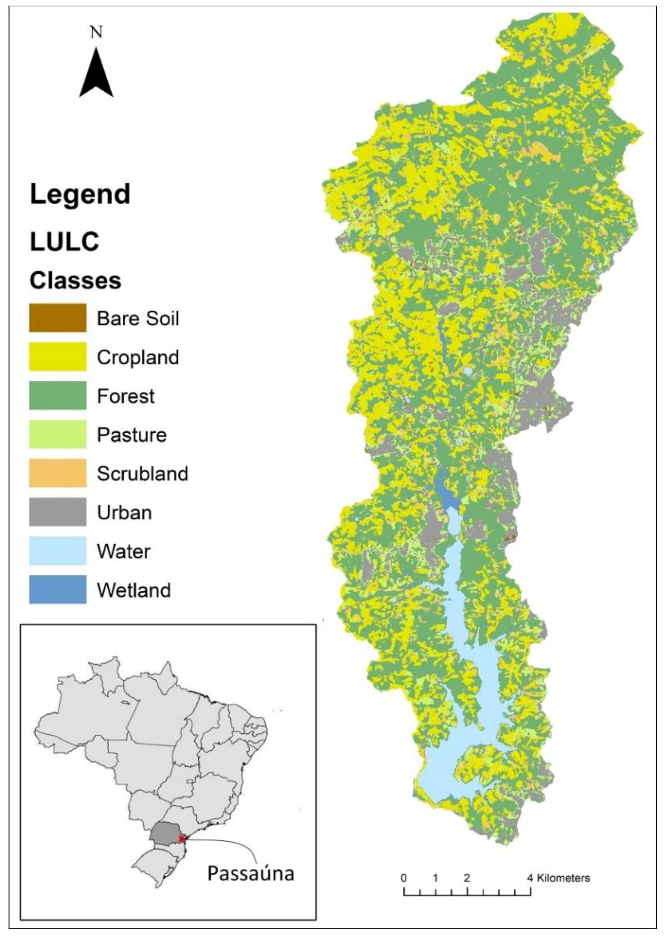
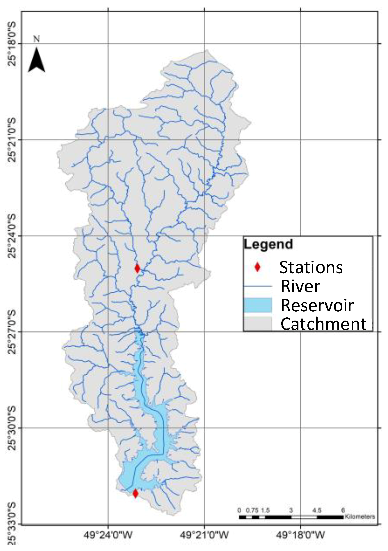
2.1. Study Area
2.2. Sediment Yield Model
- A is the soil loss at the investigated area
- L is the slope length factor
- S is the slope steepness factor
- R is the rainfall-runoff erosivity factor
- C is the cover management factor
- K is the soil erodibility factor
- P is the support practice factor
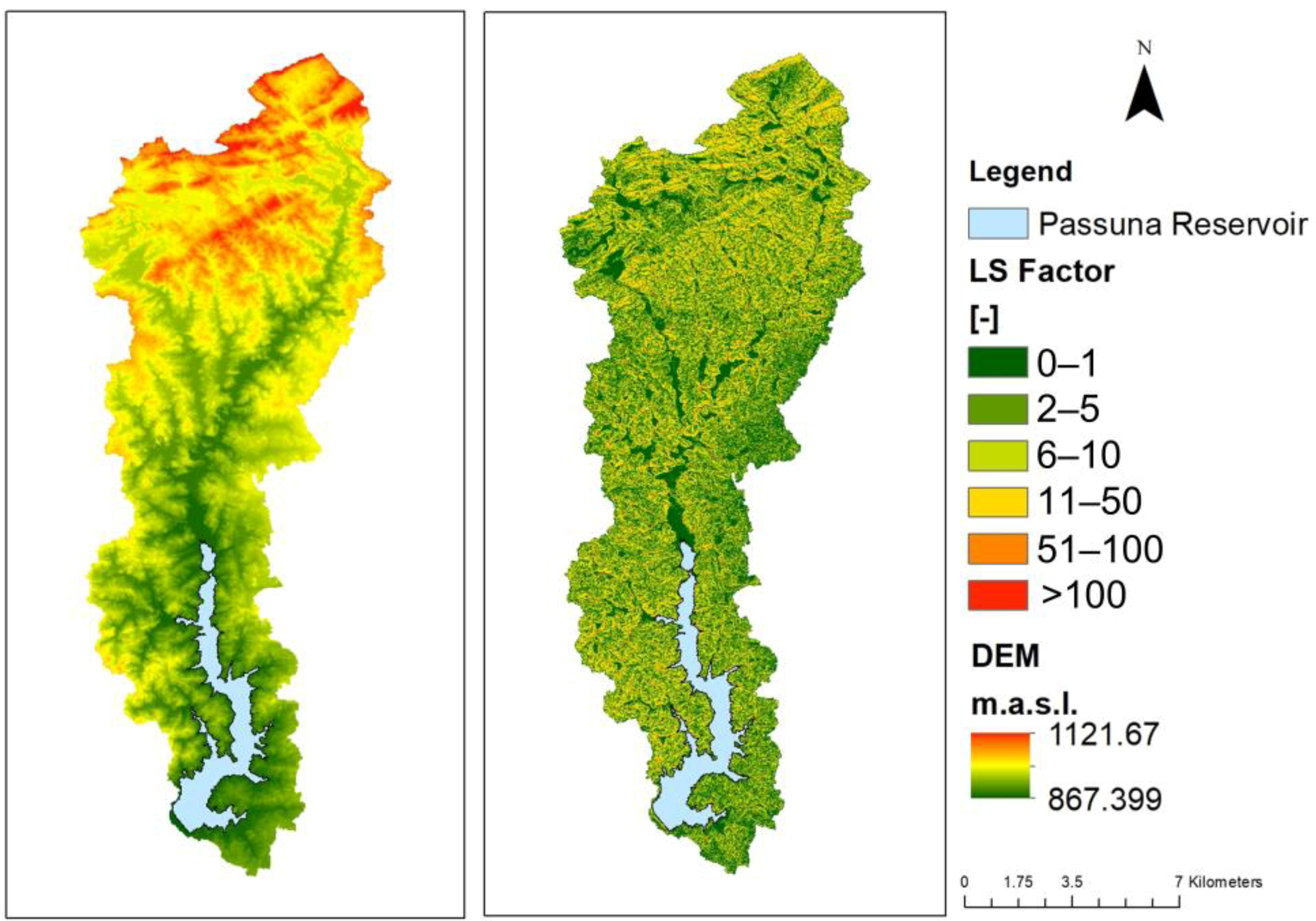
2.2.1. Topographic Factor LS
- Si is the slope factor calculated from terrain slope in radians as showed belowS = 10.8 sin θ + 0.03 when θ < 9%S = 16.8 sin θ − 0.50 when θ > 9%
- D is the gridcell dimension
- Ai-in is the contributing area (m2) at the inlet of a grid cell which is computed from the d-infinity flow direction method
- xi = |sin ai| + |cos ai| when θ > 9%and ai is the aspect direction for grid cell i
- m is the length exponent factor (Table 1)
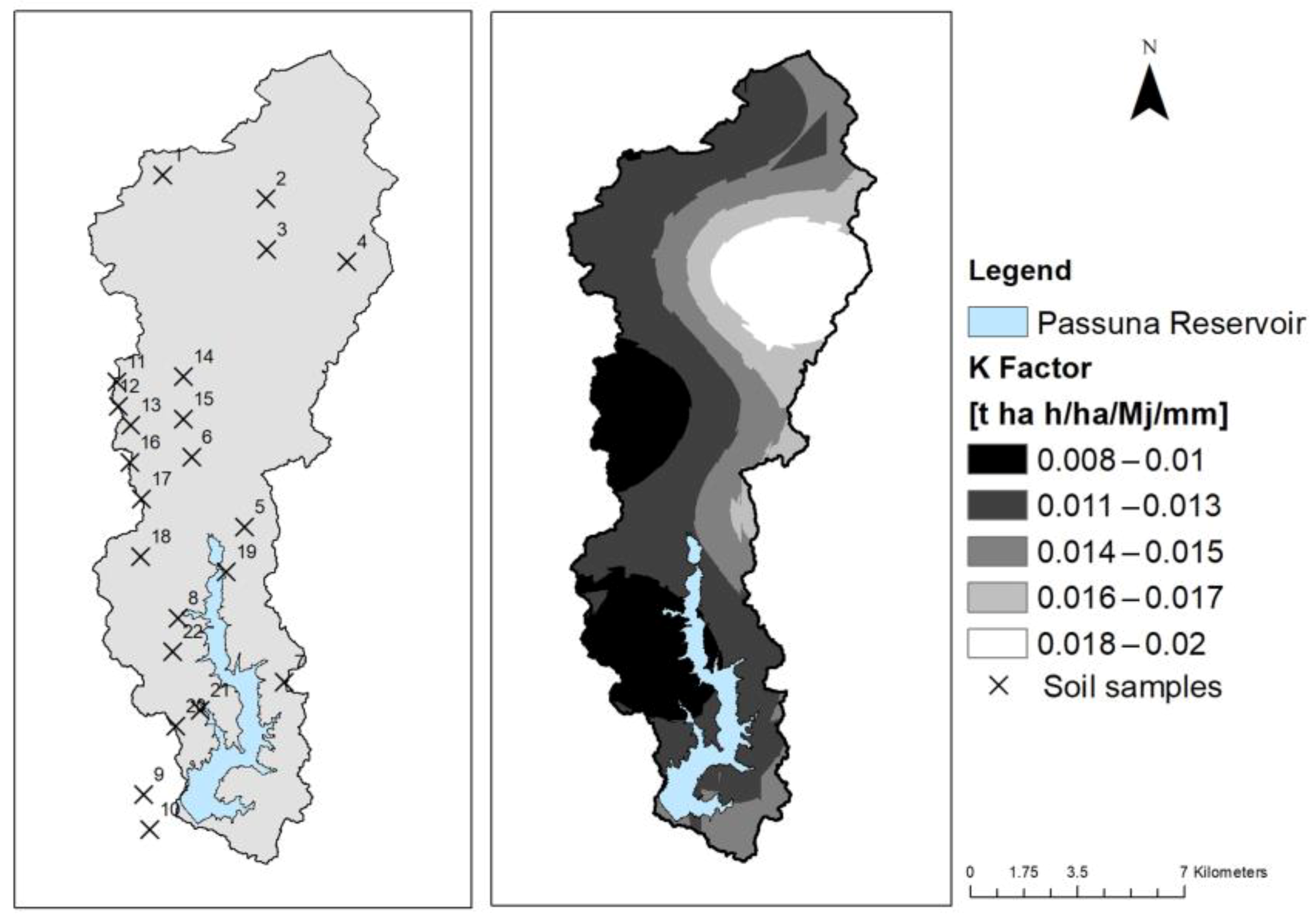
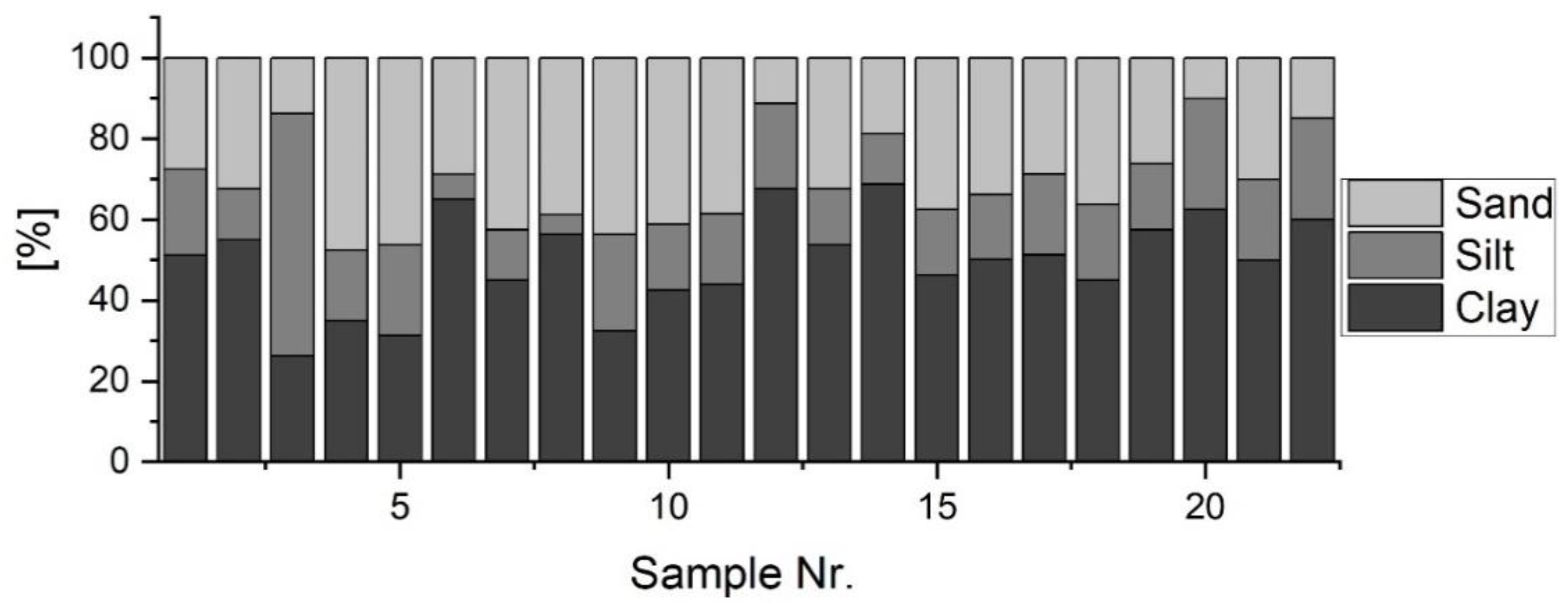
2.2.2. Soil Erodibility Factor K
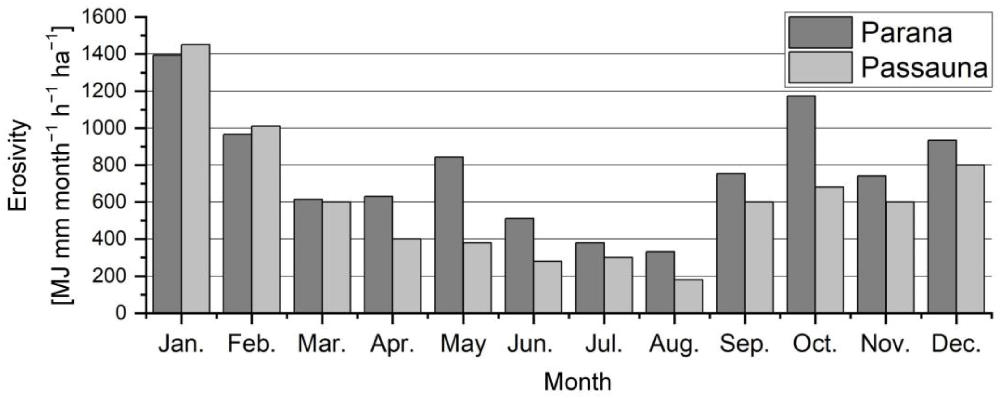
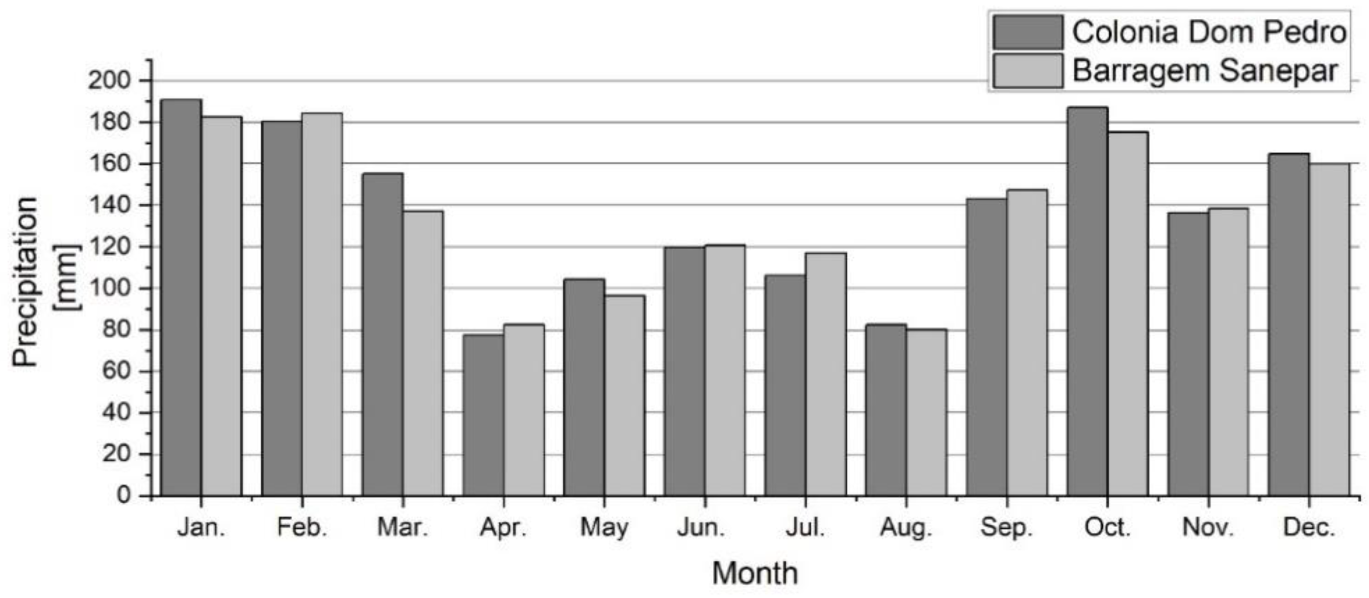
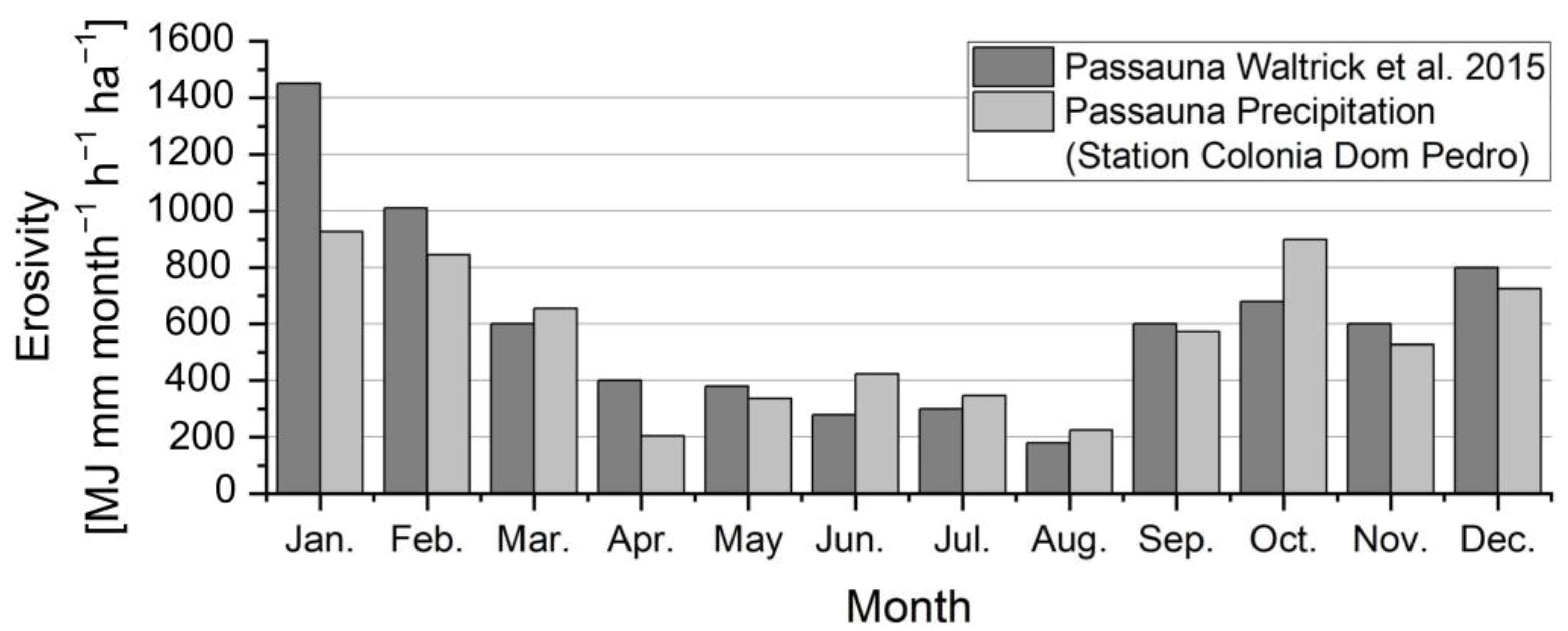
2.2.3. Rain Erosivity Factor R
- Based on literature findings
- 2.
- Based on Pluviometric Data of Daily Frequency
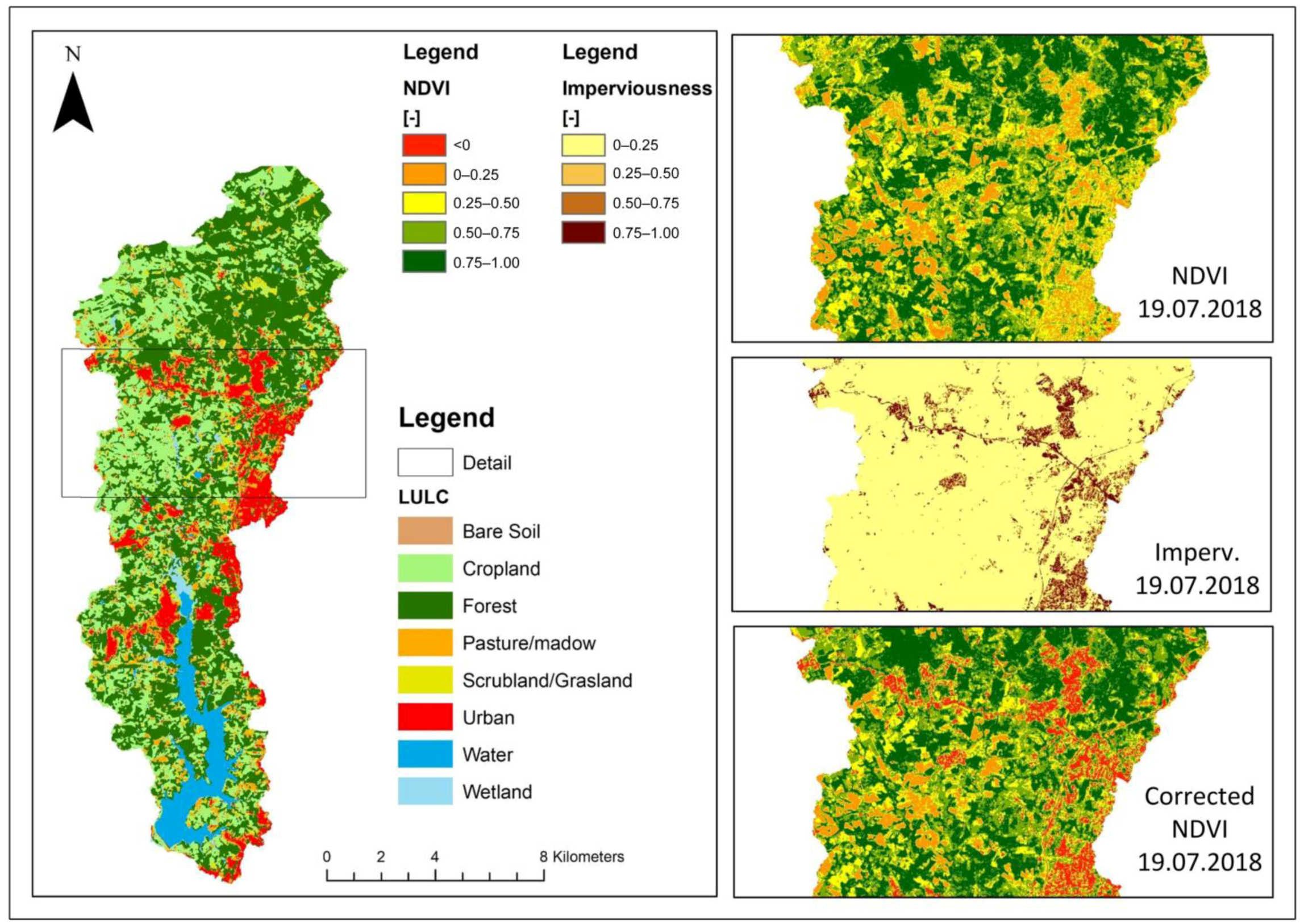
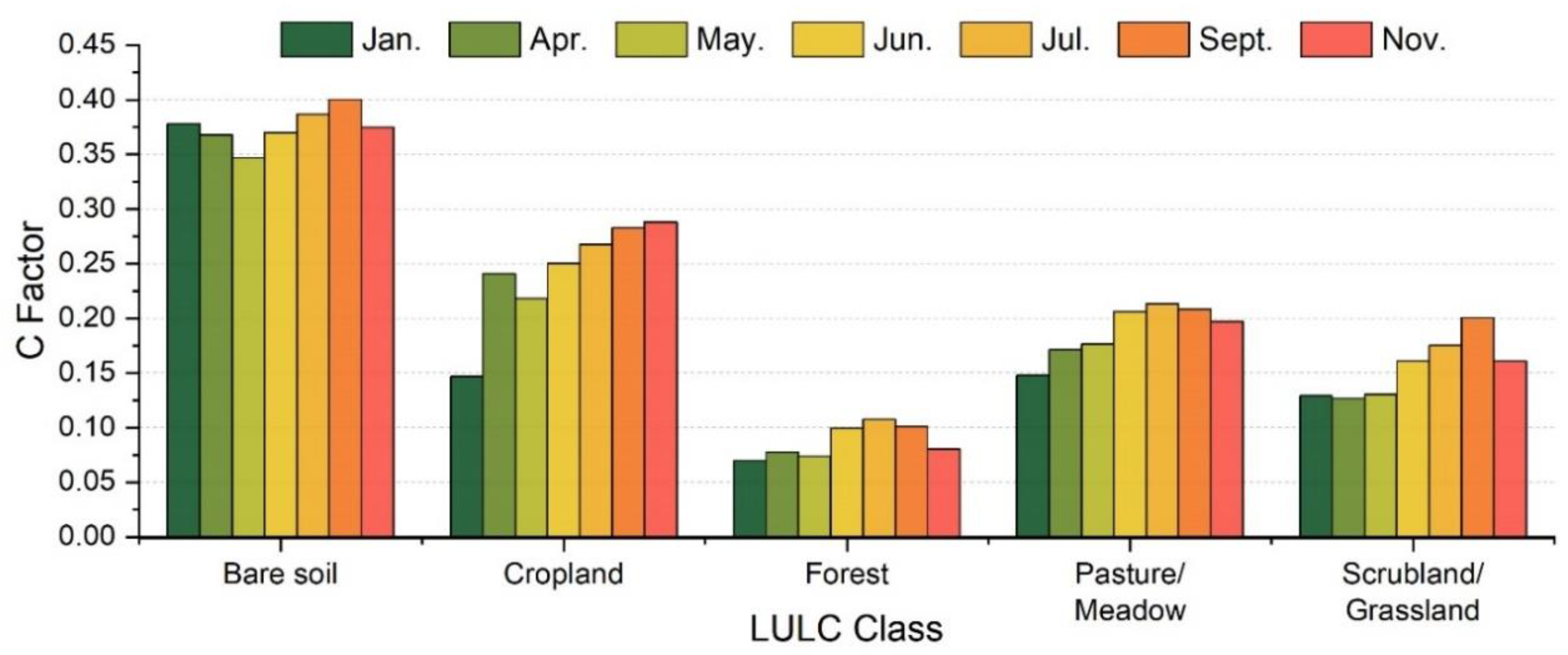
2.2.4. Cover and Management Factor C
2.2.5. Conservation Practices Factor P
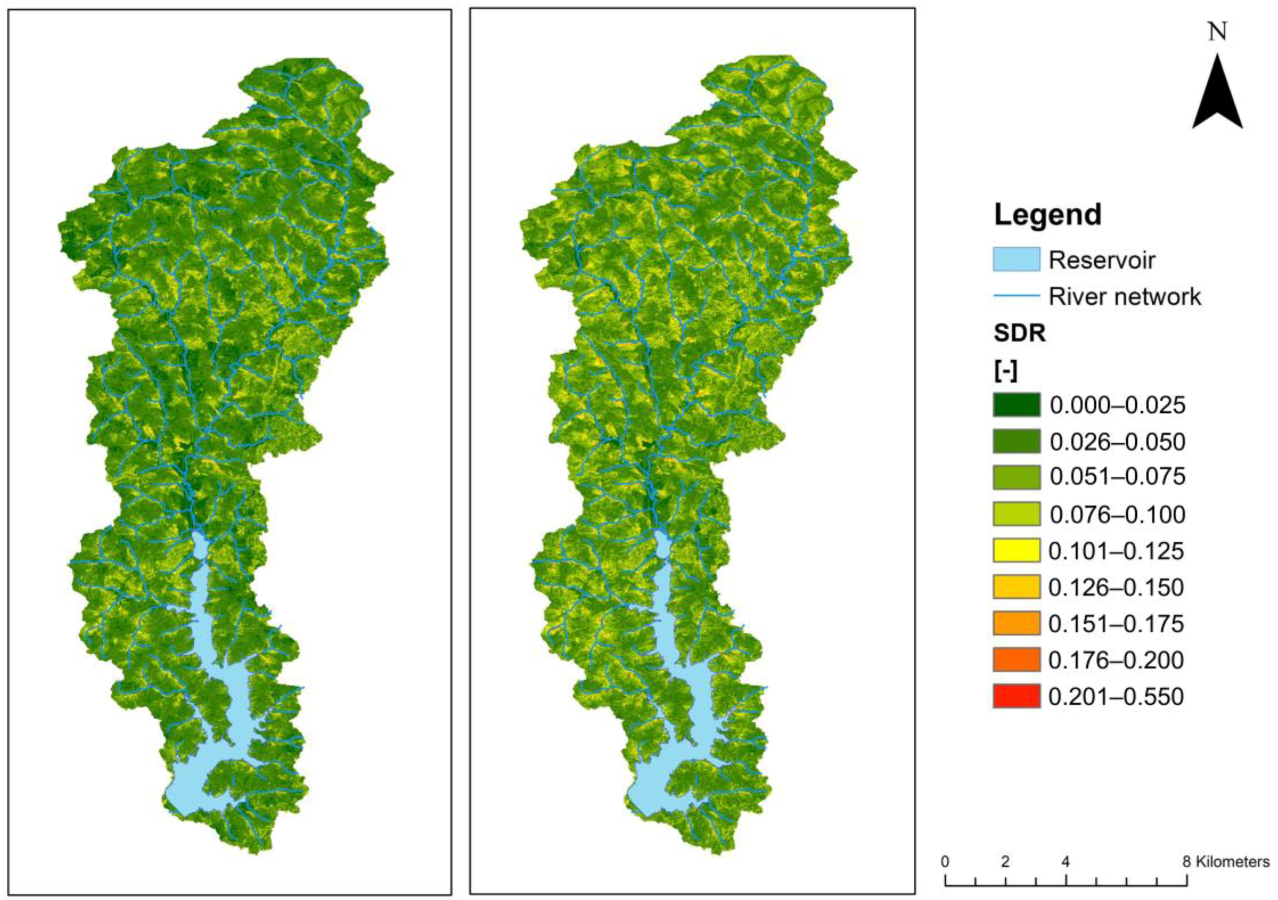
2.2.6. Sediment Delivery Model
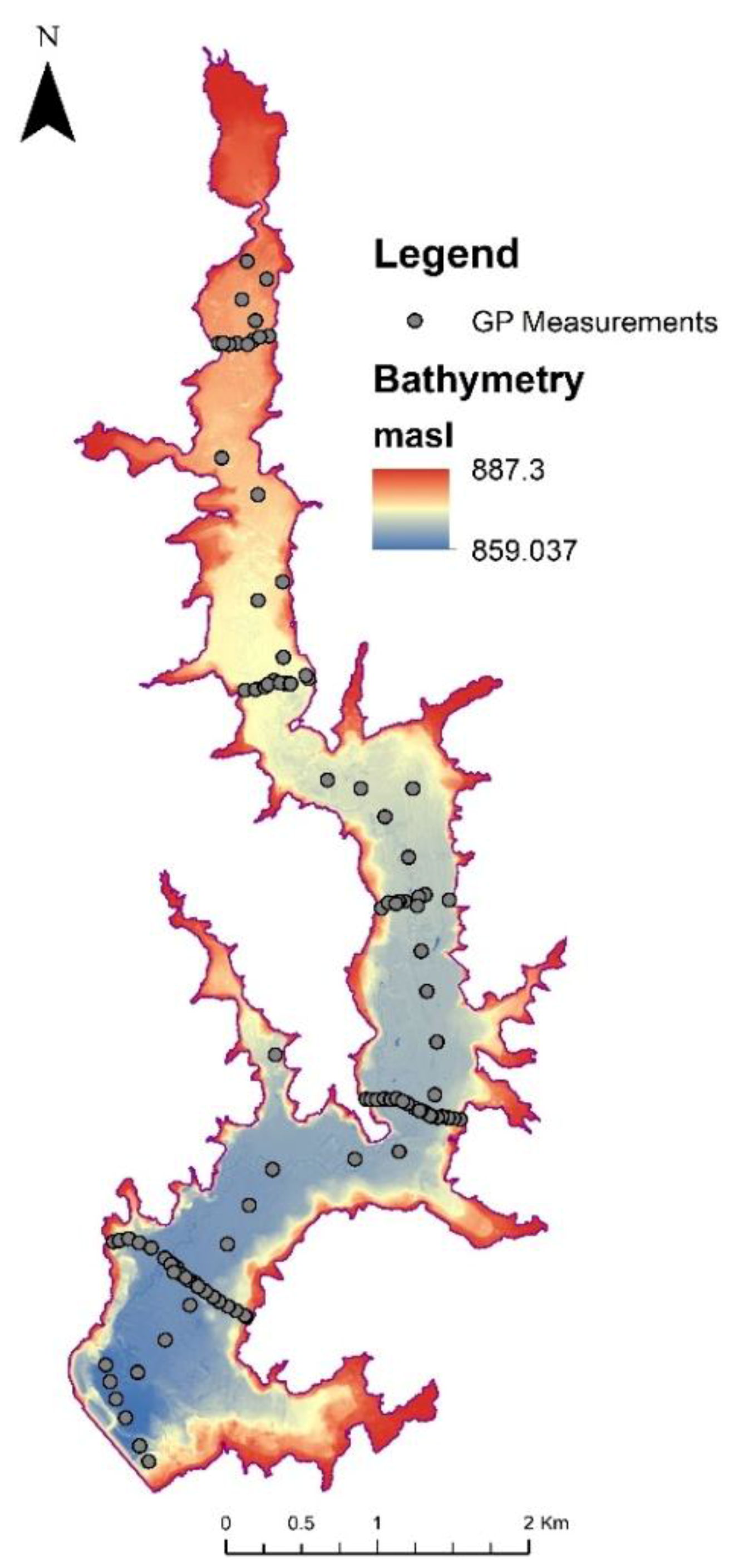
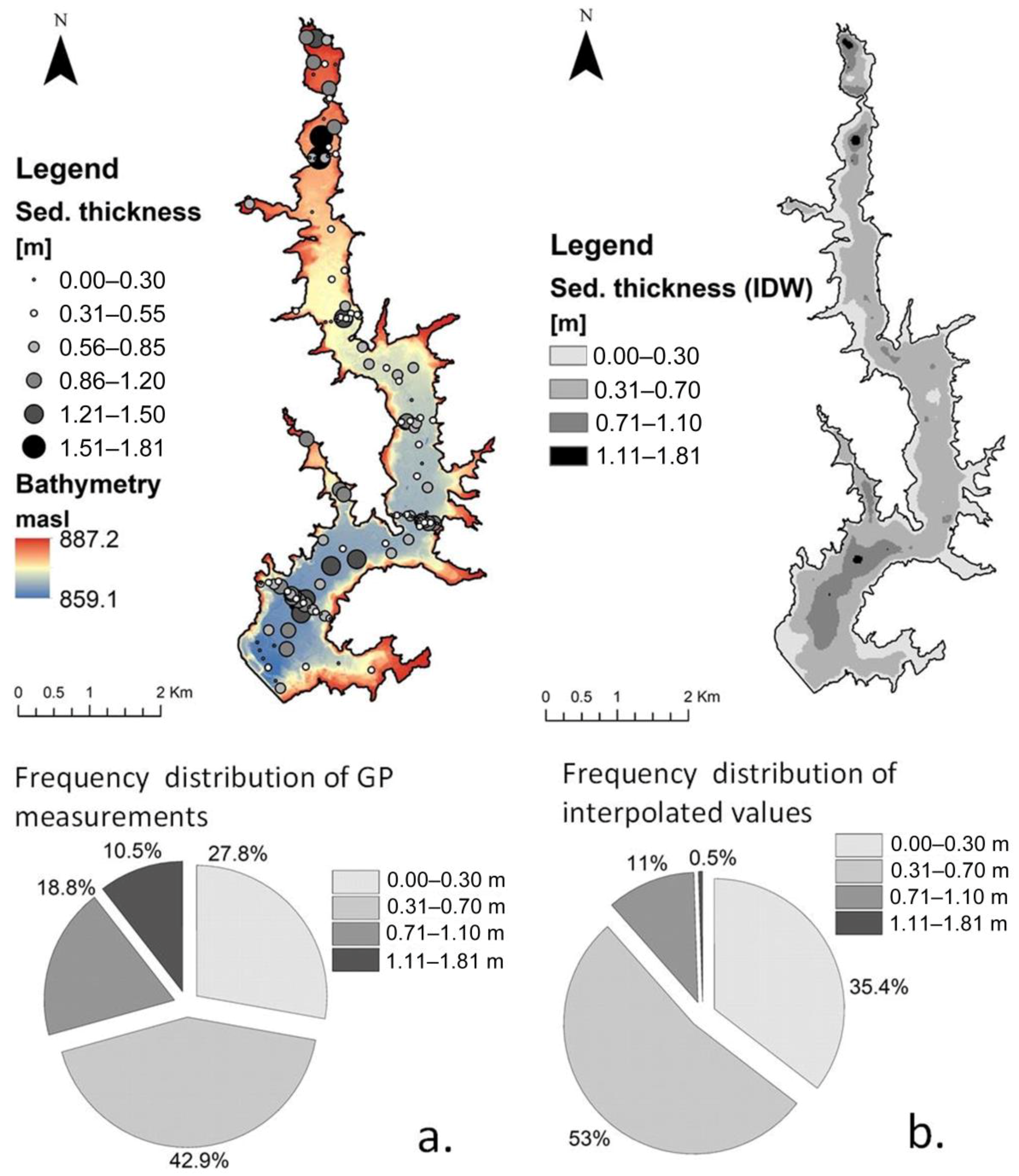
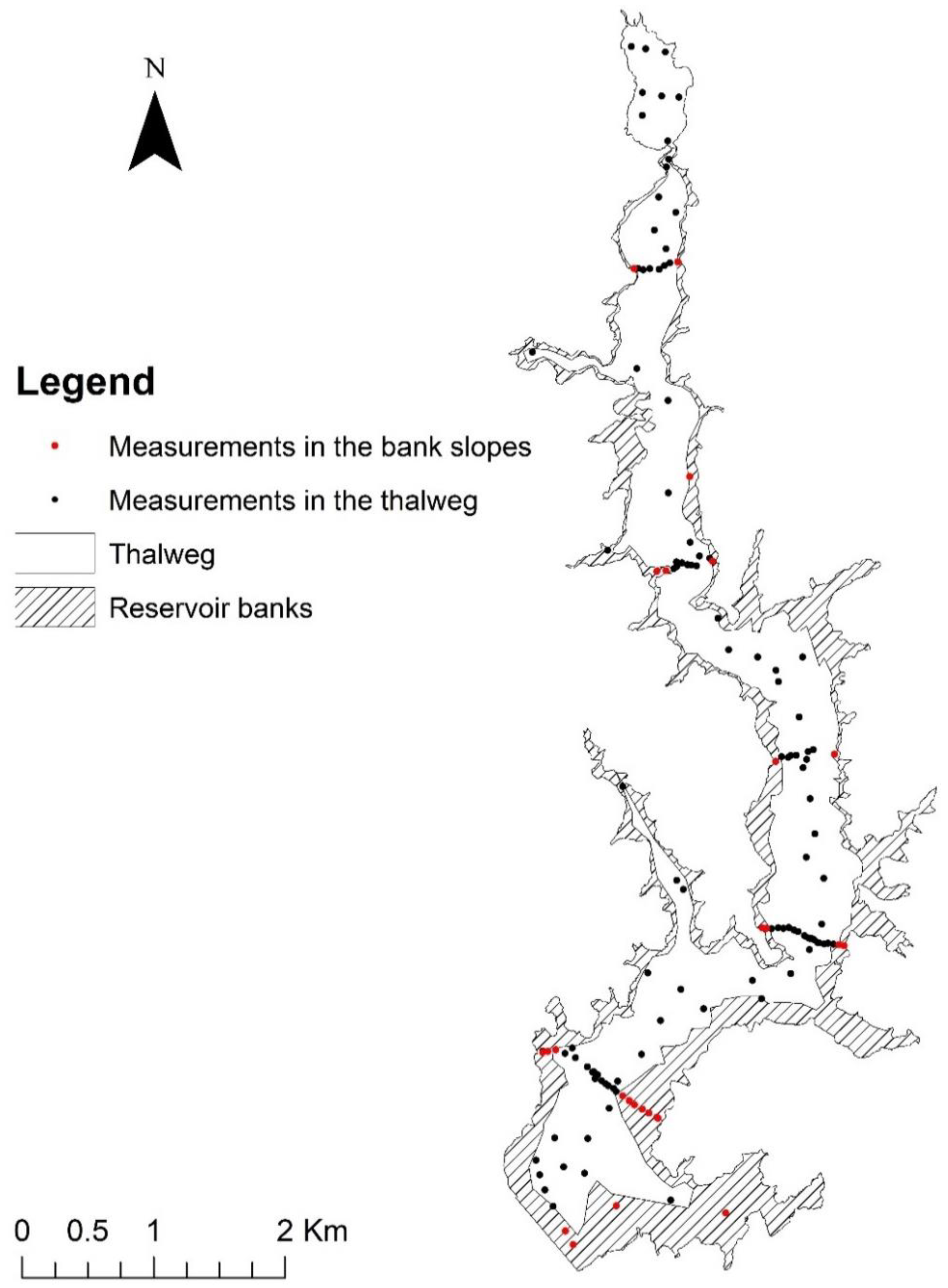
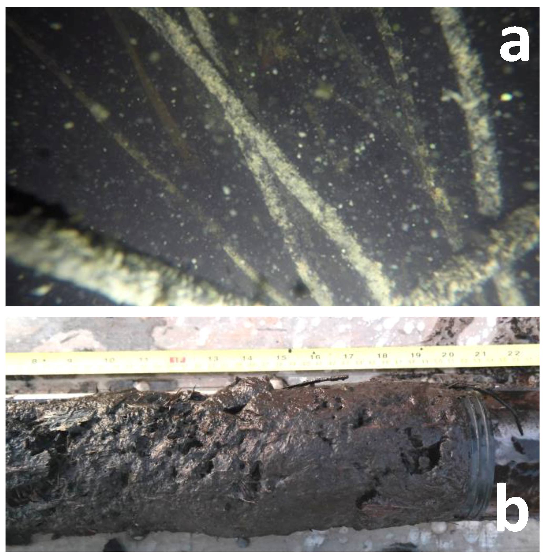
2.3. Sediment in the Reservoir
3. Results
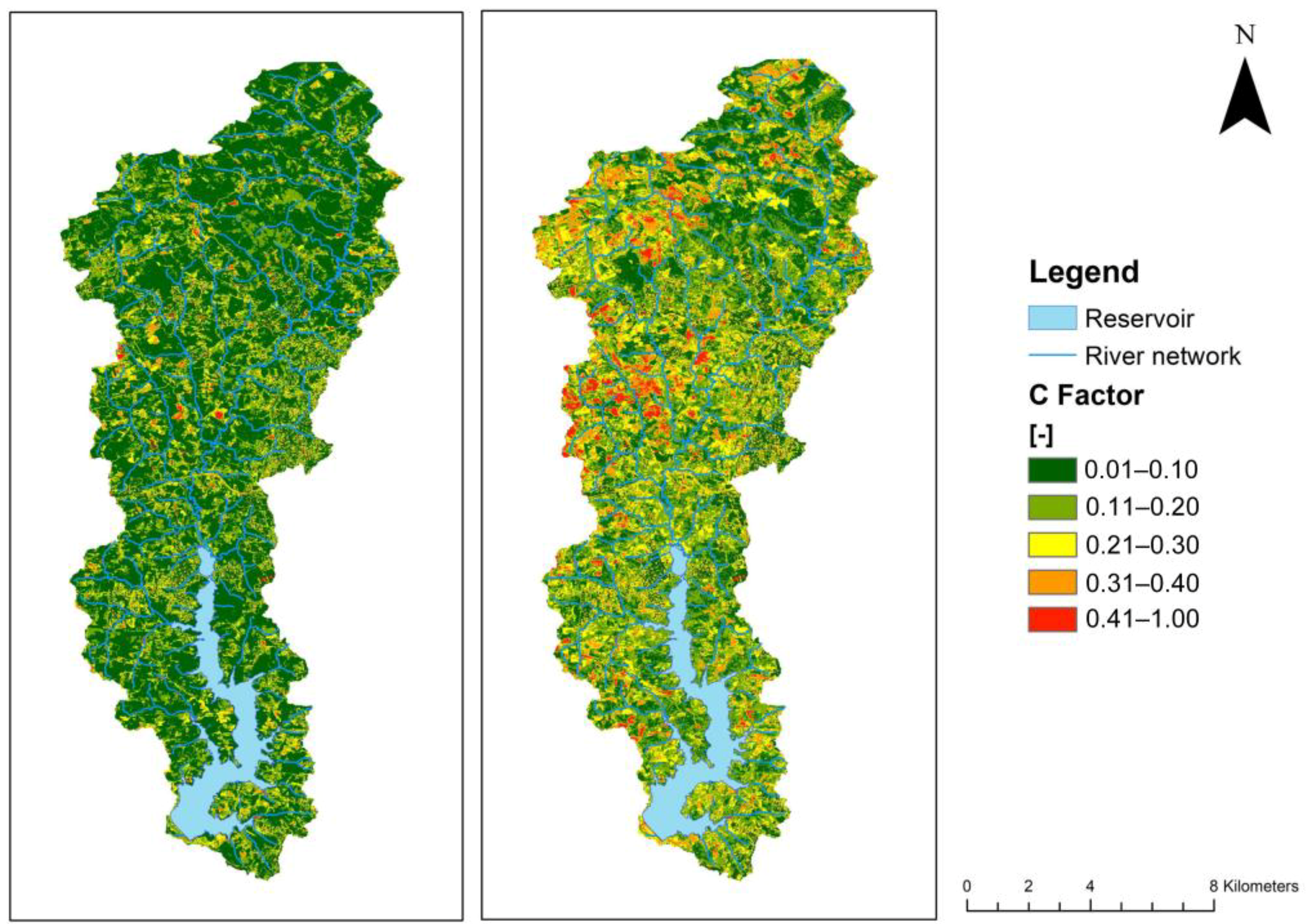
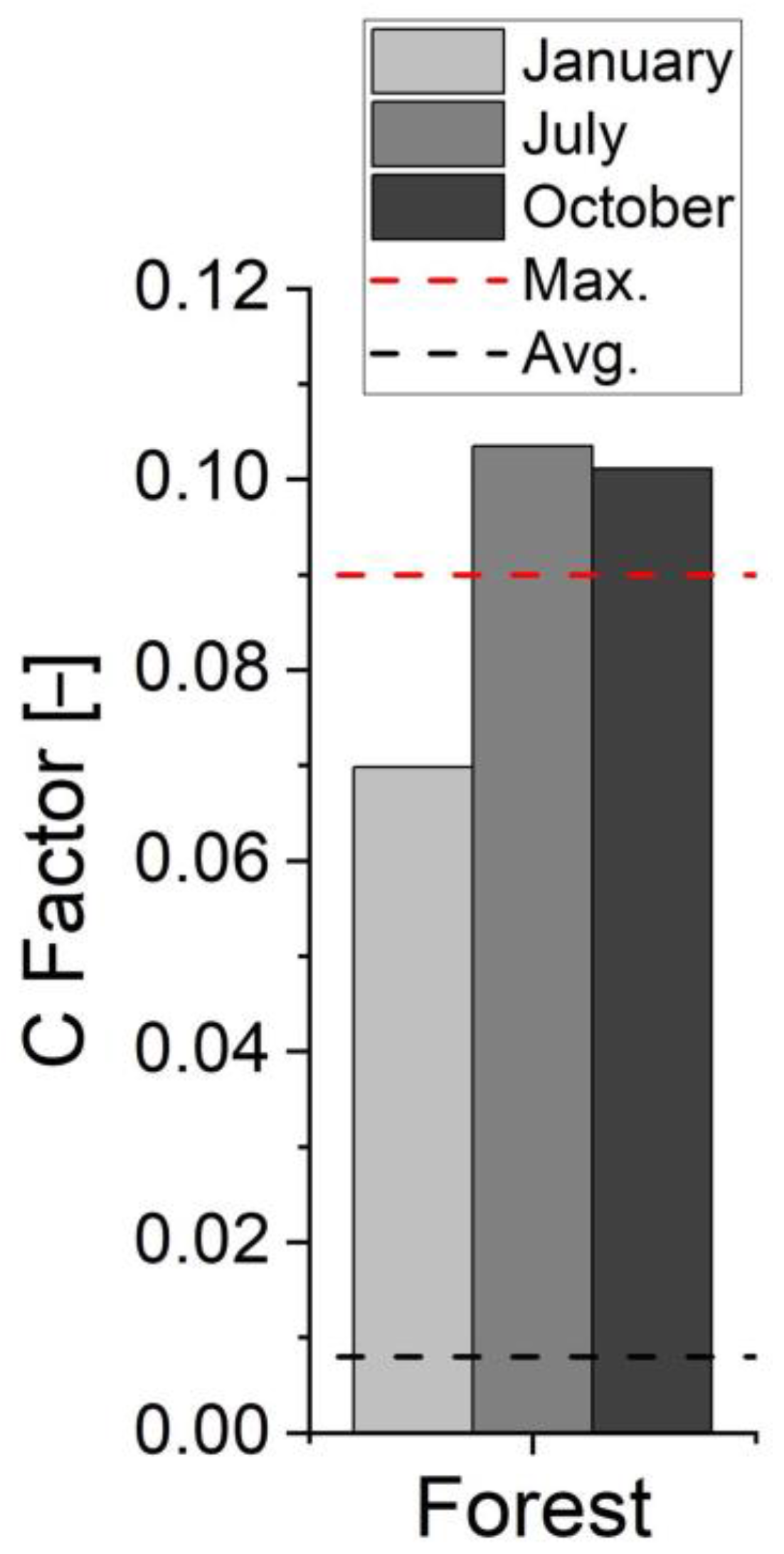
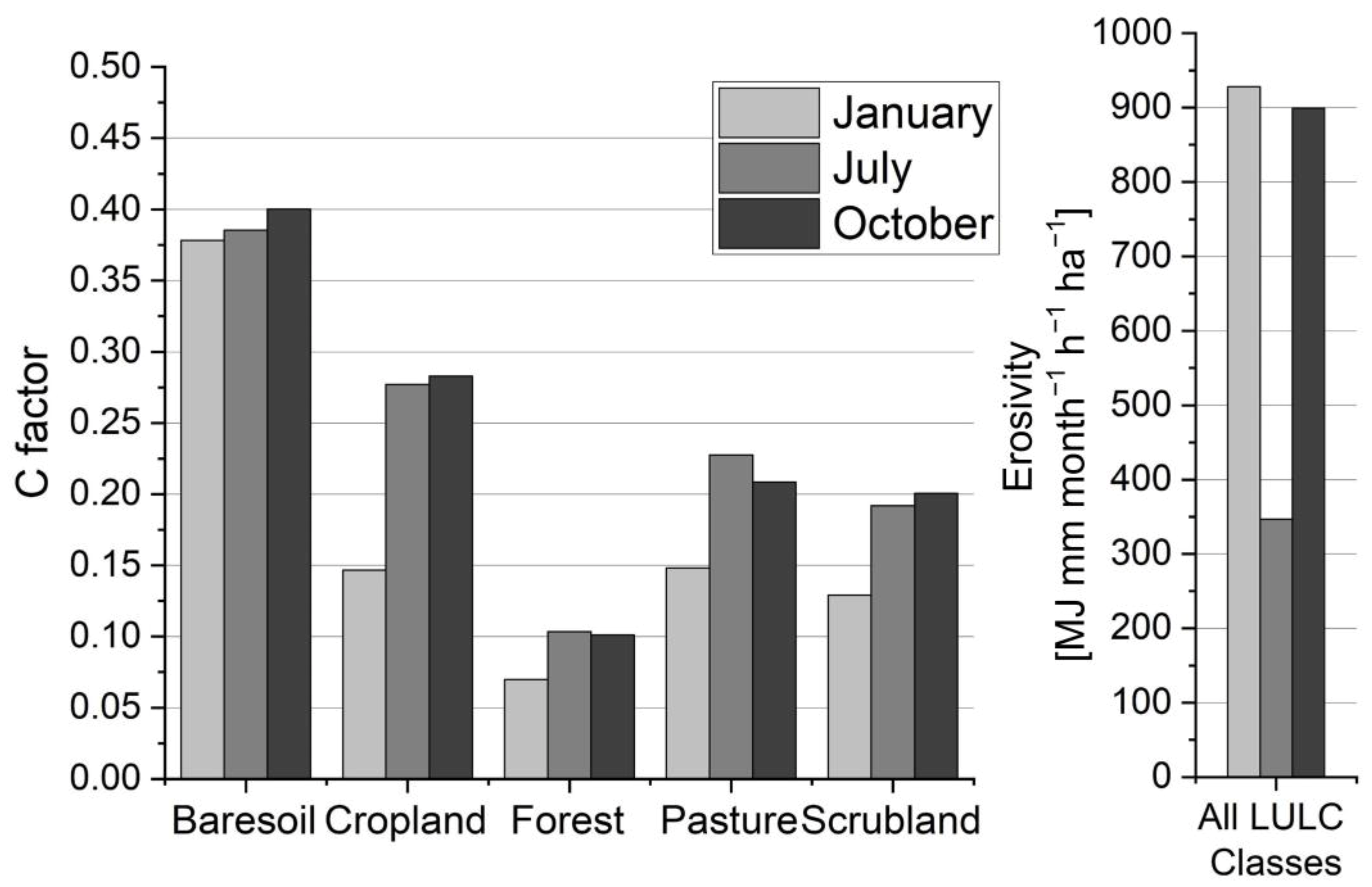
3.1. C Factor
3.2. R Factor
3.3. K Factor
3.4. Sediment Delivery Ratio
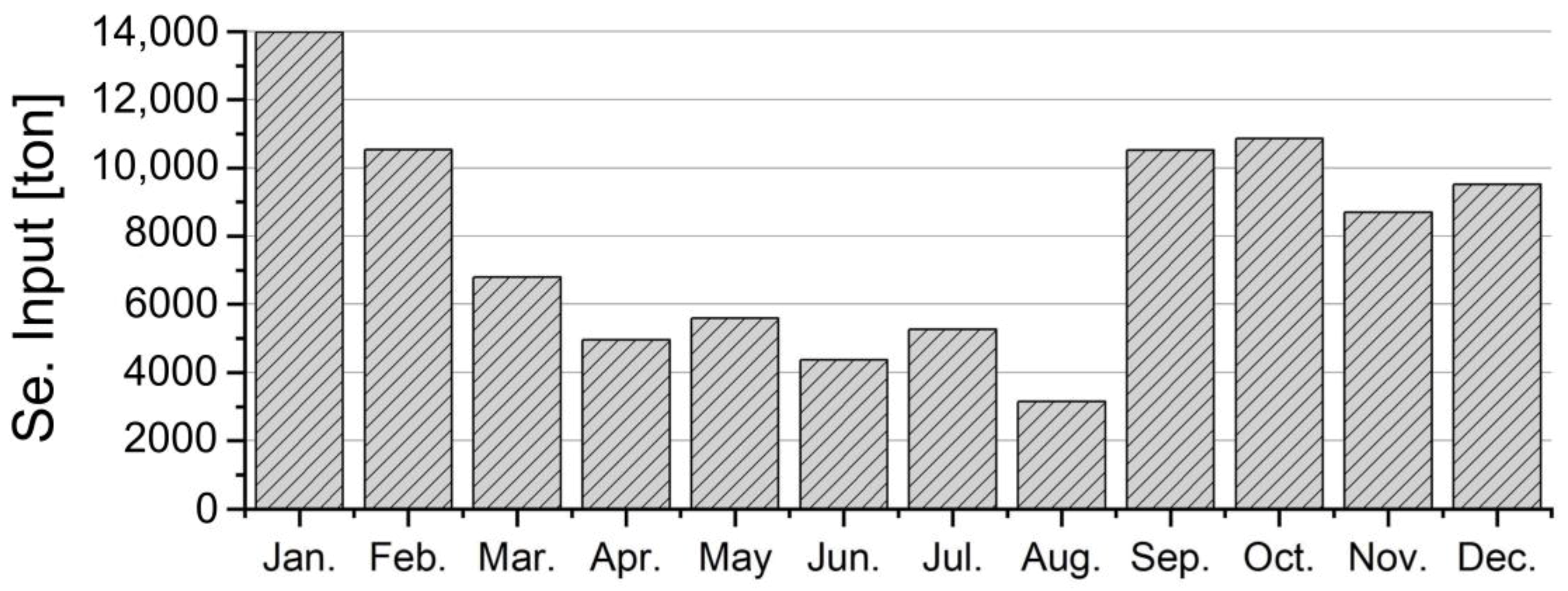
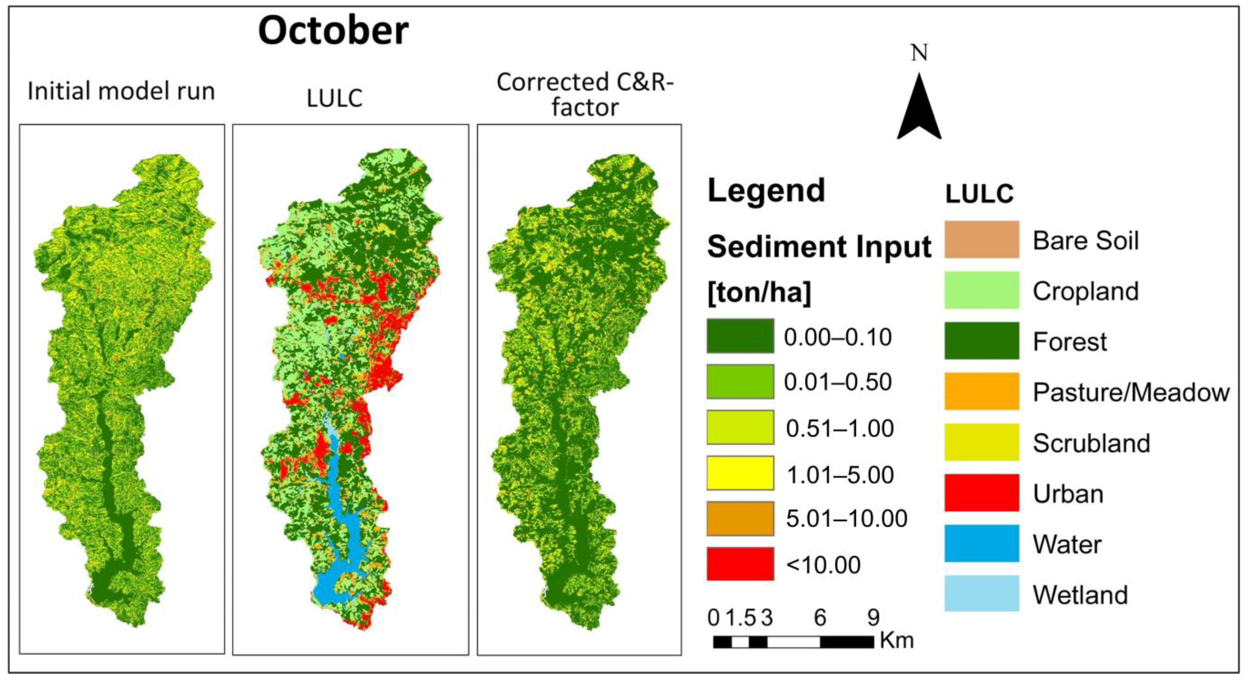
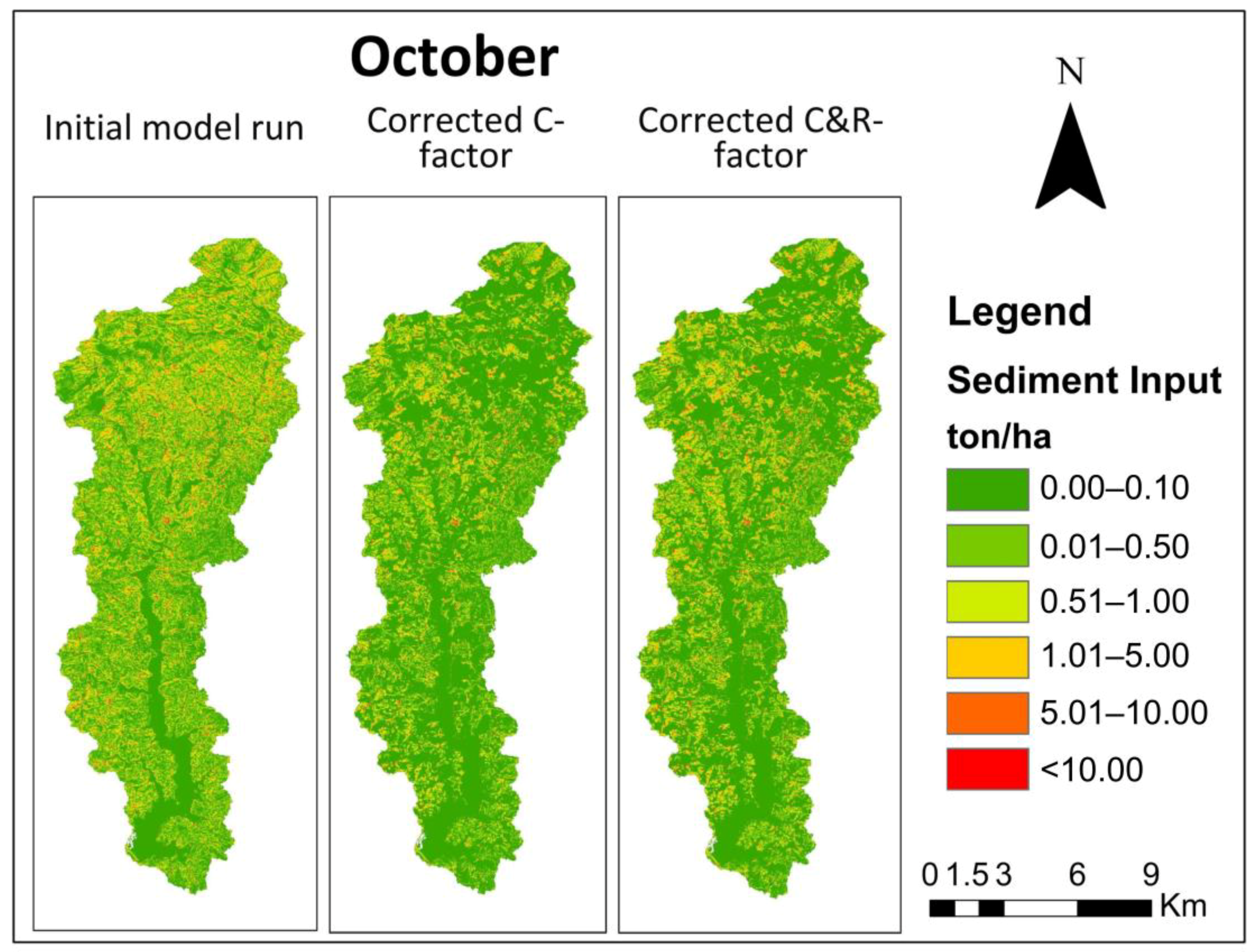
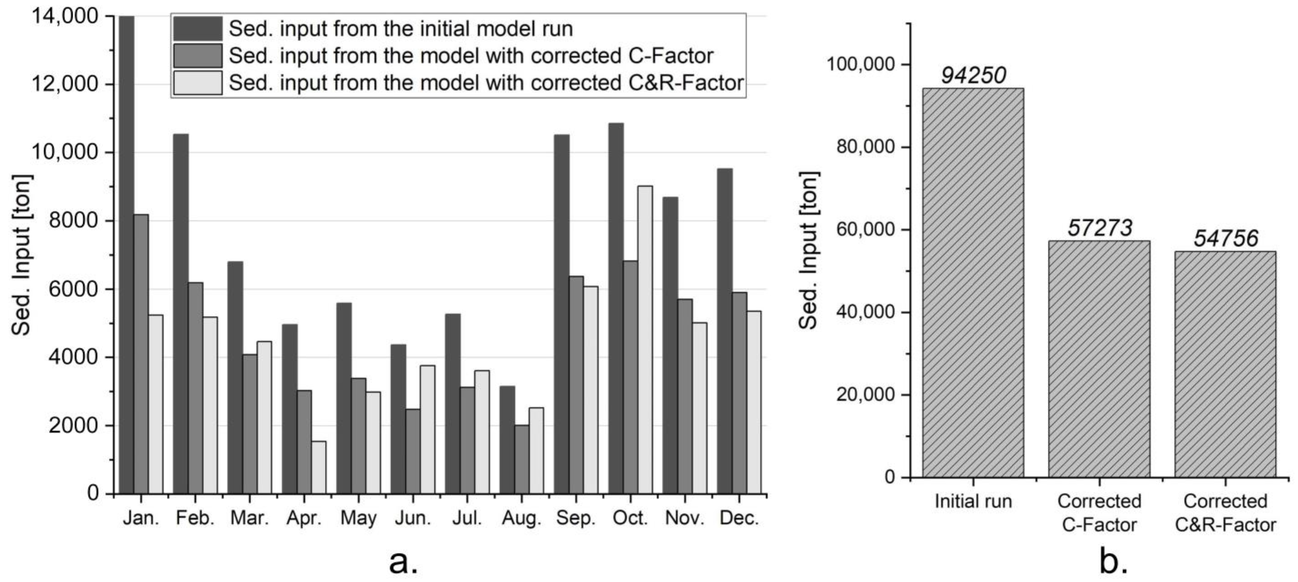
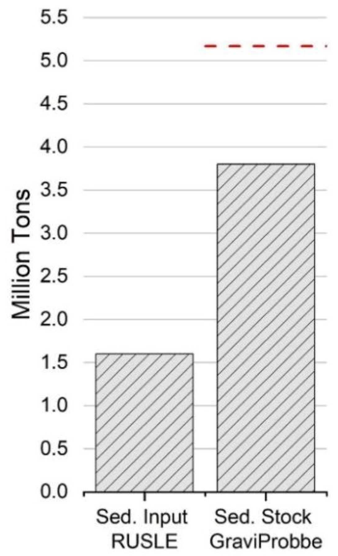
3.5. Sediment Input—Initial Model Run
3.6. Reservoir Sediment Stock
4. Discussion
4.1. Comparison of the Approach to Literature Findings
4.2. Sediment Input from Catchment vs. Reservoir Sediment Stock
4.3. Limitations of Normalized Difference Vegetation Index (NDVI)-Based Approaches for the Estimation of the C Factor in Forested Areas
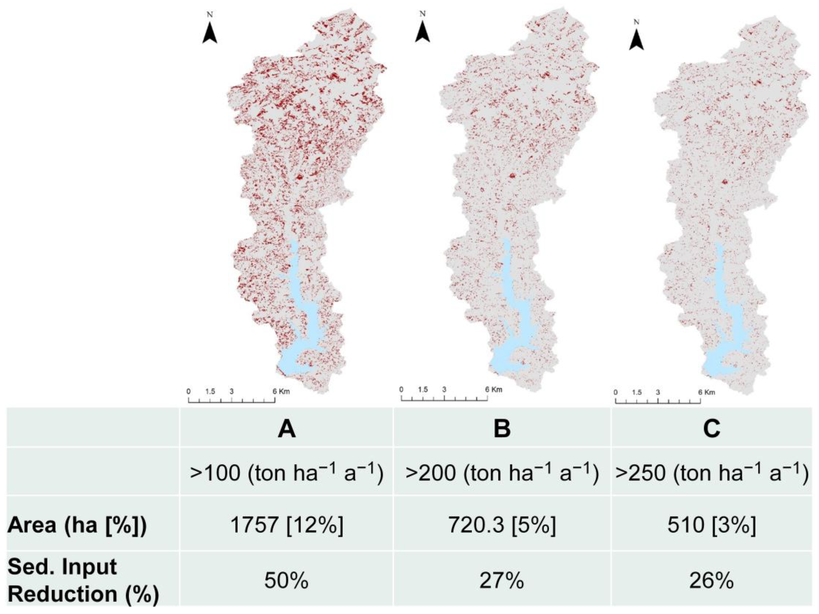
4.4. Management Implications
4.5. Uncertainties of the Sediment Yield Model for the Passaúna Catchment
4.6. Benefits from the Integration of Sentinel-2 Data in Erosion Modeling
5. Conclusions
Author Contributions
Funding
Institutional Review Board Statement
Informed Consent Statement
Acknowledgments
Conflicts of Interest
References
- Montgomery, D.R. Dirt: The Erosion of Civilizations; Univ of California Press: Berkeley, CA, USA, 2012; ISBN 0520272900. [Google Scholar]
- Dotterweich, M. The history of human-induced soil erosion: Geomorphic legacies, early descriptions and research, and the development of soil conservation—A global synopsis. Geomorphology 2013, 201, 1–34. [Google Scholar] [CrossRef]
- Reusser, L.; Bierman, P.; Rood, D. Quantifying human impacts on rates of erosion and sediment transport at a landscape scale. Geology 2015, 43, 171–174. [Google Scholar] [CrossRef]
- Hooke, R.B. On the history of humans as geomorphic agents. Geology 2000, 28, 843–846. [Google Scholar] [CrossRef]
- Pimentel, D.; Allen, J.; Beers, A.; Guinand, L.; Linder, R.; McLaughlin, P.; Meer, B.; Musonda, D.; Perdue, D.; Poisson, S.; et al. World Agriculture and Soil Erosion. BioScience 1987, 37, 277–283. [Google Scholar] [CrossRef]
- FAO. Soil Erosion: The Greatest Challenge to Sustainable Soil Management; FAO: Rome, Italy, 2019. [Google Scholar]
- Quinton, J.N.; Govers, G.; van Oost, K.; Bardgett, R.D. The impact of agricultural soil erosion on biogeochemical cycling. Nat. Geosci. 2010, 3, 311–314. [Google Scholar] [CrossRef] [Green Version]
- Merritt, W.S.; Letcher, R.A.; Jakeman, A.J. A review of erosion and sediment transport models. Environ. Model. Softw. 2003, 18, 761–799. [Google Scholar] [CrossRef]
- Verstraeten, G.; Poesen, J. Using sediment deposits in small ponds to quantify sediment yield from small catchments: Possibilities and limitations. Earth Surf. Process. Landf. 2002, 27, 1425–1439. [Google Scholar] [CrossRef]
- Boix-Fayos, C.; de Vente, J.; Martínez-Mena, M.; Barberá, G.G.; Castillo, V. The impact of land use change and check-dams on catchment sediment yield. Hydrol. Process. 2008, 22, 4922–4935. [Google Scholar] [CrossRef]
- Odhiambo, B.K.; Ricker, M.C. Spatial and isotopic analysis of watershed soil loss and reservoir sediment accumulation rates in Lake Anna, Virginia, USA. Environ. Earth Sci. 2012, 65, 373–384. [Google Scholar] [CrossRef]
- Sotiri, K.; Hilgert, S.; Mannich, M.; Bleninger, T.; Fuchs, S. Implementation of comparative detection approaches for the accurate assessment of sediment thickness and sediment volume in the Passaúna Reservoir. J. Environ. Manag. 2021. [Google Scholar] [CrossRef]
- Carneiro, C.; Kelderman, P.; Irvine, K. Assessment of phosphorus sediment–water exchange through water and mass budget in Passaúna Reservoir (Paraná State, Brazil). Environ. Earth Sci. 2016, 75, 564. [Google Scholar] [CrossRef]
- Wischmeier, W.H.; Smith, D.D. Predicting Rainfall Erosion Losses: A Guide to Conservation Planning; U.S. Department of Agriculture: Washington, DC, USA, 1978. [Google Scholar]
- Renard, K.G.; Foster, G.R.; Weesies, D.K.; McCool, D.K.; Yoder, D.C. Predicting Soil Erosion by Water: A Guide to Conservation Planning with the Revised Universal Soil Loss Equation (RUSLE); FAO: Washington, DC, USA, 1997. [Google Scholar]
- Desmet, P.J.J.; Govers, G. Modelling topographic potential for erosion and deposition using GIS. Int. J. Geogr. Inf. Sci. 1997, 11, 603–610. [Google Scholar] [CrossRef]
- inVEST- Natural Capital Project. Available online: http://releases.naturalcapitalproject.org/invest-userguide/latest/sdr.html (accessed on 30 January 2020).
- Abdo, H.; Salloum, J. Spatial assessment of soil erosion in Alqerdaha basin (Syria). Modeling Earth Syst. Environ. 2017, 3, 26. [Google Scholar] [CrossRef]
- Marques, V.; Ceddia, M.; Antunes, M.; Carvalho, D.; Anache, J.; Rodrigues, D.; Oliveira, P.T. USLE K-Factor Method Selection for a Tropical Catchment. Sustainability 2019, 11, 1840. [Google Scholar] [CrossRef] [Green Version]
- Clemente, E.; Oliveira, A.; Fontana, A.; Martins, A.; Schuler, A.; Fidalgo, E.; Monteiro, J. Erodibilidade dos Solos da Região Serrana do Rio de Janeiro Obtida por Diferentes Equações de Predição Indireta; Embrapa Solos: Rio de Janeiro, Brazil, 2017. [Google Scholar]
- Schick, J.; Bertol, I.; Cogo, N.P.; González, A.P. Erodibilidade de um Cambissolo Húmico sob chuva natural. Rev. Bras. Ciênc. Solo 2014, 38, 1906–1917. [Google Scholar] [CrossRef] [Green Version]
- Silva, M.; Freitas, P.; Blancaneaux, P.; Curi, N.; de Lima, J. Relaçao entre parâmetros da chuva e perdas de solo e determinaçao da erodibilidade de um latossolo vermelho-escuro em Goiânia (GO). Rev. Bras. Ciência Solo 1997, 21, 131–137. [Google Scholar]
- Gee, G.W.; Or, D. 2.4 Particle-size analysis. Methods Soil Anal. Part 4 Phys. Methods 2002, 5, 255–293. [Google Scholar]
- Bouyoucos, G.J. The clay ratio as a criterion of susceptibility of soils to erosion. J. Am. Soc. Agron. 1935, 27, 738–741. [Google Scholar] [CrossRef] [Green Version]
- Rufino, R.L.; Biscaia, R.; Merten, G.H. Determinação do potencial erosivo da chuva do estado do Paraná, através de pluviometria: Terceira aproximação. Rev. Bras. Ciência Solo 1993, 17, 439–444. [Google Scholar]
- Waltrick, P.C.; Machado, M.A.d.M.; Dieckow, J.; Oliveira, D.d. Estimativa da Erosividade de Chuvas no Estado do Paraná Pelo Método da Pluviometria: Atualização Com Dados de 1986 A 2008. Rev. Bras. Ciência Solo 2015, 39, 256–267. [Google Scholar] [CrossRef] [Green Version]
- Lombardi Neto, F.; Moldenhauer, W.C. Rainfall Erosivity: Its Distribution and Relationship with Soil Loss at Campinas, Brasil. Bragantia 1992, 51, 189–196. [Google Scholar] [CrossRef] [Green Version]
- Risse, L.M.; Nearing, M.A.; Laflen, J.M.; Nicks, A.D. Error Assessment in the Universal Soil Loss Equation. Soil Sci. Soc. Am. J. 1993, 57, 825–833. [Google Scholar] [CrossRef]
- Ferreira, V.A.; Weesies, G.A.; Yoder, D.C.; Foster, G.R.; Renard, K.G. The site and condition specific nature of sensitivity analysis. J. Soil Water Conserv. 1995, 50, 493–497. [Google Scholar]
- Estrada-Carmona, N.; Harper, E.B.; DeClerck, F.; Fremier, A.K. Quantifying model uncertainty to improve watershed-level ecosystem service quantification: A global sensitivity analysis of the RUSLE. Int. J. Biodivers. Sci. Ecosyst. Serv. Manag. 2017, 13, 40–50. [Google Scholar] [CrossRef]
- Nearing, M.A.; Romkens, M.J.M.; Norton, L.D.; Stott, D.E.; Rhoton, F.E.; Laflen, J.M.; Flanagan, D.C.; Alonso, C.V.; Binger, R.L.; Dabney, S.M. Measurements and models of soil loss rates. Science 2000, 290, 1300–1301. [Google Scholar] [CrossRef]
- Almagro, A.; Thomé, T.C.; Colman, C.B.; Pereira, R.B.; Marcato Junior, J.; Rodrigues, D.B.B.; Oliveira, P.T.S. Improving cover and management factor (C-factor) estimation using remote sensing approaches for tropical regions. Int. Soil Water Conserv. Res. 2019, 7, 325–334. [Google Scholar] [CrossRef]
- da Silva Santos, L. Sensitivity of Sediment Budget Calculations for an Applicable Reservoir’s Lifetime. Master’s Thesis, Karlsruhe Institute of Technology, Karlsruhe, Germany, 2019. [Google Scholar]
- Durigon, V.L.; Carvalho, D.F.; Antunes, M.A.H.; Oliveira, P.T.S.; Fernandes, M.M. NDVI time series for monitoring RUSLE cover management factor in a tropical watershed. Int. J. Remote Sens. 2014, 35, 441–453. [Google Scholar] [CrossRef]
- Panagos, P.; Borrelli, P.; Meusburger, K.; van der Zanden, E.H.; Poesen, J.; Alewell, C. Modelling the effect of support practices (P-factor) on the reduction of soil erosion by water at European scale. Environ. Sci. Policy 2015, 51, 23–34. [Google Scholar] [CrossRef]
- Borrelli, P.; Robinson, D.A.; Fleischer, L.R.; Lugato, E.; Ballabio, C.; Alewell, C.; Meusburger, K.; Modugno, S.; Schütt, B.; Ferro, V.; et al. An assessment of the global impact of 21st century land use change on soil erosion. Nat. Commun. 2017, 8, 2013. [Google Scholar] [CrossRef] [Green Version]
- Breiman, L. Random Forests. Mach. Learn. 2001, 46, 5–32. [Google Scholar] [CrossRef] [Green Version]
- Tucker, C.J.; Sellers, P.J. Satellite Remote Sensing of Primary Production. Int. J. Remote Sens. 1986, 7, 1395–1416. [Google Scholar] [CrossRef]
- Ridd, M.K. Exploring a V-I-S (vegetation-impervious surface-soil) model for urban ecosystem analysis through remote sensing: Comparative anatomy for cities†. Int. J. Remote Sens. 1995, 16, 2165–2185. [Google Scholar] [CrossRef]
- Kaspersen, P.; Fensholt, R.; Drews, M. Using Landsat Vegetation Indices to Estimate Impervious Surface Fractions for European Cities. Remote Sens. 2015, 7, 8224–8249. [Google Scholar] [CrossRef] [Green Version]
- van der Knijff, J.M.F.; Jones, R.J.A.; Montanarella, L. Soil Erosion Risk Assessment in Italy; Citeseer: Princeton, NJ, USA, 1999. [Google Scholar]
- Walling, D.E. The sediment delivery problem. J. Hydrol. 1983, 65, 209–237. [Google Scholar] [CrossRef]
- Vigiak, O.; Borselli, L.; Newham, L.T.H.; McInnes, J.; Roberts, A.M. Comparison of conceptual landscape metrics to define hillslope-scale sediment delivery ratio. Geomorphology 2012, 138, 74–88. [Google Scholar] [CrossRef]
- Croke, J.; Mockler, S.; Fogarty, P.; Takken, I. Sediment concentration changes in runoff pathways from a forest road network and the resultant spatial pattern of catchment connectivity. Geomorphology 2005, 68, 257–268. [Google Scholar] [CrossRef]
- Cavalli, M.; Trevisani, S.; Comiti, F.; Marchi, L. Geomorphometric assessment of spatial sediment connectivity in small Alpine catchments. Geomorphology 2013, 188, 31–41. [Google Scholar] [CrossRef]
- Hamel, P.; Chaplin-Kramer, R.; Sim, S.; Mueller, C. A new approach to modeling the sediment retention service (InVEST 3.0): Case study of the Cape Fear catchment, North Carolina, USA. Sci. Total Environ. 2015, 524–525, 166–177. [Google Scholar] [CrossRef]
- de Rosa, P.; Cencetti, C.; Fredduzzi, A. A GRASS Tool for the Sediment Delivery Ratio Mapping. PeerJ 2016. [Google Scholar] [CrossRef]
- Grauso, S.; Pasanisi, F.; Tebano, C. Assessment of a Simplified Connectivity Index and Specific Sediment Potential in River Basins by Means of Geomorphometric Tools. Geosciences 2018, 8, 48. [Google Scholar] [CrossRef] [Green Version]
- Borselli, L.; Cassi, P.; Torri, D. Prolegomena to sediment and flow connectivity in the landscape: A GIS and field numerical assessment. Catena 2008, 75, 268–277. [Google Scholar] [CrossRef]
- Jamshidi, R.; Dragovich, D.; Webb, A.A. Distributed empirical algorithms to estimate catchment scale sediment connectivity and yield in a subtropical region. Hydrol. Process. 2014, 28, 2671–2684. [Google Scholar] [CrossRef]
- Saavedra, C. Estimating Spatial Patterns of Soil Erosion and Deposition in the Andean Region Using Geo-Information Techniques. Ph.D. Thesis, Wageningen University, Wageningen, The Netherlands, 2005. [Google Scholar]
- Elçi, Ş.; Bor, A.; Çalışkan, A. Using numerical models and acoustic methods to predict reservoir sedimentation. Lake Reserv. Manag. 2009, 25, 297–306. [Google Scholar] [CrossRef] [Green Version]
- Krasa, J.; Dostal, T.; Jachymova, B.; Bauer, M.; Devaty, J. Soil erosion as a source of sediment and phosphorus in rivers and reservoirs—Watershed analyses using WaTEM/SEDEM. Environ. Res. 2019, 171, 470–483. [Google Scholar] [CrossRef] [PubMed]
- True, D.G. Penetration of Projectiles into Seafloor Soils; Defense Technical Information Center: Fort Belvoir, VA, USA, 1975. [Google Scholar]
- Beard, R.M. A Penetrometer for Deep Seafloor Exploration. In Proceedings of the OCEANS 81, Boston, MA, USA, 16–18 September 1981. [Google Scholar]
- Osler, J.; Furlong, A.; Christian, H.; Lamplugh, M. The integration of the free fall cone penetrometer (FFCPT) with the moving vessel profiler (MVP) for the rapid assessment of seabed characteristics. Int. Hydrogr. Rev. 2006, 7, 45–54. [Google Scholar]
- Stoll, R.D. Measuring sea bed properties using static and dynamic penetrometers. In Proceedings of the Sixth International Conference on Civil Engineering in the Oceans, Baltimore, MD, USA, 20–22 October 2004; pp. 386–395. [Google Scholar]
- Stark, N.; Kopf, A. Detection and Quantification of Sediment Remobilization Processes Using a Dynamic Penetrometer. In Proceedings of the OCEANS'11 MTS/IEEE KONA, Waikoloa, HI, USA, 19–22 September 2011. [Google Scholar]
- Seifert, A.; Kopf, A. Modified dynamic CPTU penetrometer for fluid mud detection. J. Geotech. Geoenviron. Eng. 2012, 138, 203–206. [Google Scholar] [CrossRef]
- Albatal, A.; Stark, N. Rapid sediment mapping and in situ geotechnical characterization in challenging aquatic areas. Limnol. Oceanogr. Methods 2017, 15, 690–705. [Google Scholar] [CrossRef]
- Hilgert, S.; Sotiri, K.; Fuchs, S. Advanced Assessment of Sediment Characteristics Based on Rheological and Hydroacoustic Measurements in a Brazilian Reservoir. In Proceedings of the 38th IAHR World Congress, Panama City, Panama, 1–6 September 2019; 2019. [Google Scholar]
- Kirichek, A.; Rutgers, R. Water Injection Dredging and Fluid Mud Trapping Pilot in the Port of Rotterdam; CEDA Dredging Days: Rotterdam, The Netherlands, 2019. [Google Scholar]
- Kirichek, A.; Shakeel, A.; Chassagne, C. Using in situ density and strength measurements for sediment maintenance in ports and waterways. J. Soils Sediments 2020. [Google Scholar] [CrossRef] [Green Version]
- Morris, G.; Fan, J. Reservoir Sedimentation Handbook; McGraw-Hill Book, Co.: New York, NY, USA, 2010. [Google Scholar]
- Rahmani, V.; Kastens, J.; deNoyelles, F.; Jakubauskas, M.; Martinko, E.; Huggins, D.; Gnau, C.; Liechti, P.; Campbell, S.; Callihan, R.; et al. Examining Storage Capacity Loss and Sedimentation Rate of Large Reservoirs in the Central U.S. Great Plains. Water 2018, 10, 190. [Google Scholar] [CrossRef] [Green Version]
- Sotiri, K.; Hilgert, S.; Fuchs, S. Sediment classification in a Brazilian reservoir: Pros and cons of parametric low frequencies. Adv. Oceanogr. Limnol. 2019, 10. [Google Scholar] [CrossRef]
- Embrapa Solos. Mapa de Solos de Estado de Parana; Embrapa Solos: Rio de Janeiro, Brazil, 2007. [Google Scholar]
- Mannigel, A.R.; de Passos, M.; Moreti, D.; da Rosa Medeiros, L. Fator erodibilidade e tolerância de perda dos solos do Estado de São Paulo. Acta Scientiarum. Agron. 2002, 24, 1335–1340. [Google Scholar] [CrossRef]
- Silva, A.; Silva, M.; Curi, N.; Avanzi, J.; Ferreira, M. Rainfall erosivity and erodibility of Cambisol (Inceptisol) and Latosol (Oxisol) in the region of Lavras, Southern Minas Gerais State, Brazil. Rev. Bras. Ciência Solo 2009, 33, 1811–1820. [Google Scholar] [CrossRef] [Green Version]
- Duraes, M.F.; de Mello, C.R.; Beskow, S. Sediment yield in Paraopeba River Basin—MG, Brazil. Int. J. River Basin Manag. 2016, 14, 367–377. [Google Scholar] [CrossRef]
- Duraes, M.; Filho, J.; Oliveira, V. Water erosion vulnerability and sediment delivery rate in upper Iguaçu river basin—Paraná. RBRH 2016, 21. [Google Scholar] [CrossRef]
- Saunitti, R.M.; Fernandes, L.A.; Bittencourt, A.V.L. Estudo do assoreamento do reservatório da barragem do rio Passaúna-Curitiba-PR. Bol. Parana. Geociências 2004, 54, 54. [Google Scholar] [CrossRef] [Green Version]
- Wagner, A. Event-Based Measurement and Mean Annual Flux Assessment of Suspended Sediment in Meso Scale Catchments. Ph.D. Thesis, Karlsruhe Institute of Technology, Karlsruhe, Germany, 2019. [Google Scholar]
- Koszelnik, P.; Gruca-Rokosz, R.; Bartoszek, L. An isotopic model for the origin of autochthonous organic matter contained in the bottom sediments of a reservoir. Int. J. Sediment Res. 2017. [Google Scholar] [CrossRef]
- Quinton, J.N. Erosion and sediment transport. In Environmental Modelling: Finding Simplicity in Complexity; John Wiley & Sons Ltd.: London UK, 2004. [Google Scholar]
- Belyaev, V.R.; Wallbrink, P.J.; Golosov, V.N.; Murray, A.S.; Sidorchuk, A.Y. A comparison of methods for evaluating soil redistribution in the severely eroded Stavropol region, southern European Russia. Geomorphology 2005, 65, 173–193. [Google Scholar] [CrossRef]
- Alewell, C.; Borrelli, P.; Meusburger, K.; Panagos, P. Using the USLE: Chances, challenges and limitations of soil erosion modelling. Int. Soil Water Conserv. Res. 2019, 7, 203–225. [Google Scholar] [CrossRef]
- Wallbrink, P.J.; Murray, A.S.; Olley, J.M.; Olive, L.J. Determining sources and transit times of suspended sediment in the Murrumbidgee River, New South Wales, Australia, using fallout 137Cs and 210Pb. Water Resour. Res. 1998, 34, 879–887. [Google Scholar] [CrossRef]
- Walling, D.E. Tracing suspended sediment sources in catchments and river systems. Sci. Total Environ. 2005, 344, 159–184. [Google Scholar] [CrossRef]
- Wilkinson, S.N.; Prosser, I.P.; Rustomji, P.; Read, A.M. Modelling and testing spatially distributed sediment budgets to relate erosion processes to sediment yields. Environ. Model. Softw. 2009, 24, 489–501. [Google Scholar] [CrossRef]
- Poesen, J.; Nachtergaele, J.; Verstraeten, G.; Valentin, C. Gully erosion and environmental change: Importance and research needs. CATENA 2003, 50, 91–133. [Google Scholar] [CrossRef]
- Poesen, J.; Vanwalleghem, T.; de Vente, J.; Knapen, A.; Verstraeten, G.; Martínez-Casasnovas, J.A. Gully Erosion in Europe; Wiley-Interscience: Hoboken, NJ, USA, 2006; ISBN 9780470859209. [Google Scholar]
- Morgan, R.P.C. Soil Erosion; Blackwell Publishing: Hoboken, NJ, USA, 1979; ISBN 0582486920. [Google Scholar]
- Werner, C.G. Soil Conservation in Kenia; Springer: Berlin/Heidelberg, Germany, 1980. [Google Scholar]
- Wang, G.; Wente, S.; Gertner, G.Z.; Anderson, A. Improvement in mapping vegetation cover factor for the universal soil loss equation by geostatistical methods with Landsat Thematic Mapper images. Int. J. Remote Sens. 2002, 23, 3649–3667. [Google Scholar] [CrossRef]
- Zhang, Y.; Yuan, J.; Liu, B. Advance in researches on vegetation cover and management factor in the soil erosion prediction model. Ying Yong Sheng Tai Xue Bao J. Appl. Ecol. 2002, 13, 1033–1036. [Google Scholar]
- Zhang, W.; Zhang, Z.; Liu, F.; Qiao, Z.; Hu, S. Estimation of the USLE Cover and Management Factor C Using Satellite Remote Sensing: A Review. In Proceedings of the 2011 19th International Conference on Geoinformatics, Shanghai, China, 24–26 June 2011. [Google Scholar]
- Panagos, P.; Borrelli, P.; Meusburger, K.; Alewell, C.; Lugato, E.; Montanarella, L. Estimating the soil erosion cover-management factor at the European scale. Land Use Policy 2015, 48, 38–50. [Google Scholar] [CrossRef]
- Sullivan, P. Overview of Cover Crops and Green Manures. 2003. Available online: https://cpb-us-e1.wpmucdn.com/blogs.cornell.edu/dist/e/4211/files/2014/04/Overview-of-Cover-Crops-and-Green-Manures-19wvmad.pdf (accessed on 30 January 2020).
- Sullivan, P. Applying the Principles of Sustainable Farming. 2003. Available online: https://ipm.ifas.ufl.edu/pdfs/Applying_the_Principles_of_Sustainable_Farming.pdf?pub=295%5D (accessed on 30 January 2020).
- SoCo Project Team. Adressing Soil Degradation in EU Agriculture: Relevant Processes, Practices and Policies. 2009. Available online: https://esdac.jrc.ec.europa.eu/ESDB_Archive/eusoils_docs/other/EUR23767_Final.pdf (accessed on 30 January 2020).
- Zalles, V.; Hansen, M.C.; Potapov, P.V.; Stehman, S.V.; Tyukavina, A.; Pickens, A.; Song, X.-P.; Adusei, B.; Okpa, C.; Aguilar, R.; et al. Near doubling of Brazil's intensive row crop area since 2000. Proc. Natl. Acad. Sci. USA 2019, 116, 428–435. [Google Scholar] [CrossRef] [Green Version]
- Zdruli, P.; Karydas, C.G.; Dedaj, K.; Salillari, I.; Cela, F.; Lushaj, S.; Panagos, P. High resolution spatiotemporal analysis of erosion risk per land cover category in Korçe region, Albania. Earth Sci. Inform. 2016, 9, 481–495. [Google Scholar] [CrossRef]
- Pham, T.G.; Degener, J.; Kappas, M. Integrated universal soil loss equation (USLE) and Geographical Information System (GIS) for soil erosion estimation in A Sap basin: Central Vietnam. Int. Soil Water Conserv. Res. 2018, 6, 99–110. [Google Scholar] [CrossRef]
- Grauso, S.; Verrubbi, V.; Peloso, A.; Zini, A.; Sciortino, M. Estimating the C-Factor of USLE/RUSLE by Means of NDVI Time-Series in Southern Latium. An Improved Correlation Model; ENEA: Rome, Italy, 2018. [Google Scholar]
- Chuenchum, P.; Xu, M.; Tang, W. Estimation of Soil Erosion and Sediment Yield in the Lancang-Mekong River Using the Modified Revised Universal Soil Loss Equation and GIS Techniques. Water 2020, 12, 135. [Google Scholar] [CrossRef] [Green Version]
- Gianinetto, M.; Aiello, M.; Polinelli, F.; Frassy, F.; Rulli, M.C.; Ravazzani, G.; Bocchiola, D.; Chiarelli, D.D.; Soncini, A.; Vezzoli, R. D-RUSLE: A dynamic model to estimate potential soil erosion with satellite time series in the Italian Alps. Eur. J. Remote Sens. 2019, 52, 34–53. [Google Scholar] [CrossRef]
- Karydas, C.; Bouarour, O.; Zdruli, P. Mapping Spatio-Temporal Soil Erosion Patterns in the Candelaro River Basin, Italy, Using the G2 Model with Sentinel2 Imagery. Geosciences 2020, 10, 89. [Google Scholar] [CrossRef] [Green Version]


| Slope % [s] | m |
|---|---|
| s < 1 | 0.2 |
| 1 < s < 3.5 | 0.3 |
| 3.5 < s < 5 | 0.4 |
| 5 < 9 | 0.5 |
| s > 9 | m = β/((1 + β)) 1 |
| Soil Class | K Factor Value (t h MJ−1 mm−1) | Soil Class |
|---|---|---|
| Haplic Inceptisol | 0.03 | [20] |
| Humic Inceptisol | 0.0175 | [21] |
| Oxisol | 0.018 | [22] |
| Land Use | Cmax | Cmin | Cmin |
|---|---|---|---|
| Bare soil | 1.000 | 0.696 | 0.100 |
| Impervious areas | 1.000 | 0.257 | 0.000 |
| High vegetation | 0.090 | 0.008 | 0.00004 |
| Low vegetation | 0.630 | 0.099 | 0.008 |
| Water | 0.000 | 0.000 | 0.000 |
| Soil Erosion Classes (Annual Mean) | Present Study (%) | [72] (%) |
|---|---|---|
| Very Slight (< 2 t ha−1 a−1) | 55 | 52.0 |
| Slight (2–5 t ha−1 a−1) | 3.5 | |
| Moderate (5–10 t ha−1 a−1) | 3.7 | |
| High (10–50 t ha−1 a−1) | 15.8 | 10.0 |
| Severe (50–100 t ha−1 a−1) | 9.0 | 5.0 |
| Very Severe (100–500 t ha−1 a−1) | 11.3 | 33.0 |
| Catastrophic (>500 t ha−1 a−1) | 1.4 |
| Factors Creating Errors | |
|---|---|
| In reservoir | Internal production |
| Existing biological stock | |
| Errors of the measuring concept | |
| Trapping efficiency of reservoir | |
| In catchment | Errors associated with RUSLE calculations |
| Errors associated with SDR calculations | |
| Non-inclusion of gully erosion in RUSLE | |
| Non-inclusion of channel erosion in RUSLE |
Publisher’s Note: MDPI stays neutral with regard to jurisdictional claims in published maps and institutional affiliations. |
© 2021 by the authors. Licensee MDPI, Basel, Switzerland. This article is an open access article distributed under the terms and conditions of the Creative Commons Attribution (CC BY) license (https://creativecommons.org/licenses/by/4.0/).
Share and Cite
Sotiri, K.; Hilgert, S.; Duraes, M.; Armindo, R.A.; Wolf, N.; Scheer, M.B.; Kishi, R.; Pakzad, K.; Fuchs, S. To What Extent Can a Sediment Yield Model Be Trusted? A Case Study from the Passaúna Catchment, Brazil. Water 2021, 13, 1045. https://doi.org/10.3390/w13081045
Sotiri K, Hilgert S, Duraes M, Armindo RA, Wolf N, Scheer MB, Kishi R, Pakzad K, Fuchs S. To What Extent Can a Sediment Yield Model Be Trusted? A Case Study from the Passaúna Catchment, Brazil. Water. 2021; 13(8):1045. https://doi.org/10.3390/w13081045
Chicago/Turabian StyleSotiri, Klajdi, Stephan Hilgert, Matheus Duraes, Robson André Armindo, Nils Wolf, Mauricio Bergamini Scheer, Regina Kishi, Kian Pakzad, and Stephan Fuchs. 2021. "To What Extent Can a Sediment Yield Model Be Trusted? A Case Study from the Passaúna Catchment, Brazil" Water 13, no. 8: 1045. https://doi.org/10.3390/w13081045