Comparison of Various Growth Curve Models in Characterizing and Predicting Water Table Change after Intensive Mine Dewatering Is Discontinued in an East Central European Karstic Area

Abstract

The modeling of karst water level fluctuations is a crucial task in the water resource management of vulnerable karstic areas. In the Transdanubian Range (East Central Europe, Hungary), from 1950 to 1990, coal and bauxite mining were carried out, with large amounts of karst water being extracted, thus lowering the water table by amounts ranging between 10 and 100 m. Since the cessation of mining activities in the early 1990s, the volume of natural recharge has exceeded the amount of dewatering, and the system has begun to return to its original undisturbed state. This apparently welcome development does, however, bring economic and technical engineering problems. The estimation and prediction of such water level changes is often tackled via the use of deterministic approaches, however, in the present case, it is also addressed with an alternative approach using trend estimation to monthly water level data from 107 karst water wells over the period 1990–2017. To approximate the change in karst water levels, (i) growth curve models were fitted to the monthly data, allowing the estimation of karst water levels, at least as far as 2030. Similarly, this was also done with (ii) deterministic modelling in order to describe the recovery process up to 2030. Specifically, measured and predicted values for karst water level were used to derive interpolated (kriged) maps to compare the forecasting power of the two approaches. Comparing the results of the trend analysis with those of the traditional deterministic modelling results, it is apparent that the two approaches predict similar spatial distribution of water levels, but slightly different future water level values.

1. Introduction

Mining has evolved with the development of humankind helping to meet the ever-increasing demand for raw materials [1,2]. However, large-scale mining activities are often associated with a number of environmental problems, such as air, noise, soil, or water pollution. Other effects of mining, such as the infrastructure required by industrial-scale activity and changes to the landscape, may persist well beyond the cessation of mining operations, even decades after the closure of the mine [3,4]. The impact on subsurface waterbodies is among the most significant of these, and this can be both qualitative and quantitative [5,6,7]. One of the most common problems is the decrease in water levels associated with over-abstraction, a widespread global phenomenon as a result of increasing extraction not only in the course of mining operations but also for drinking water. In Australia, e.g., the groundwater system was observed over a 36-year period in the Jarrah forest, where bauxite mining took place. On the basis of the observations there, it was revealed that 11 years after the cessation of mining (and thus water abstraction), the water level had returned to the pre-disturbance state [8]. Dewatering due to mining is a major issue in Asia as well. In a sand-grave mine in Kazan, Turkey, the 30 years of over-abstraction led to the extreme depletion of the aquifer, and even, in places, to its complete removal [9]. In the Heilongdong spring area of China, changes in groundwater levels due to dewatering occasioned by long-term coal mining were examined using different statistical methods, e.g., trend analysis. Results revealed that as an effect of the mining activity, the groundwater level in the area had dropped and the discharge of springs decreased significantly [10]. This is a general negative effect occurring in other vast coal fields in North China [11,12,13]. However, it is important to recognize that the change in water level associated with mining activities can occur not only as a decrease of the water level but also, after the closure of a mine, as a very significant increase. This increase after the halt in dewatering has an adverse effect on the environment [14,15], including the generally fragile karst aquifers in such an area (e.g., [12]). The mine water can rapidly recover after closure and could cause flooding of already urbanized areas (e.g., [16]), adjacent mines (e.g., [17,18]).

In practice, deterministic models are often used for estimating such mining-related groundwater level changes [19,20,21]. The application of numerical models in the case of mines established in karst areas can be particularly problematic, as karst systems are highly heterogeneous, usually with a complex flow system [22,23], a key factor which should be taken into consideration in their study. Furthermore, in case of groundwater level prediction, it may be worth comparing the results of different approaches.

1.1. Mining Water Extraction, a Central-Eastern European Example

As part of the Soviet planned economy, mining played a prominent industrial role in many countries of the former Soviet Bloc, which was monitored, and annual targets set by state organizations (the State Planning Committee) [24]. In East Central and Eastern Europe, as a result of the socioeconomic changes in the post-Soviet countries in 1989/1990, mining activities were abandoned in many places [25,26] and, in line with this, large-scale mining water abstraction has also been moderated.

In this process, Hungary was no exception. In relation to the closure of mines, one of the most well-known cases in Hungary is the disappearance of springs around Tata [27]. The use of Tata spring waters dates back almost two millennia, to the Romans, who used these springs [28]. By the end of the 20th century, Tata had become a popular spa, as a result of which the infrastructure had also developed significantly [29]. The development of the spa town was interrupted by the mining water abstraction. Water has been pumped in the nearby town of Tatabánya since the 1920s. The situation became so serious that by the early 1950s, a shortage of drinking water occurred [27].

There were other significant regional focal points of the bauxite and coal mining. These mining centers were located in the vicinity of Nyirád, Iszkaszentgyörgy, Tatabánya, and Dorog (Figure 1). To provide a continuous water supply for mining, abstraction was required, reaching 700 m³min⁻¹ by the beginning of the 1960s and even 800 m³min⁻¹ for some years [30]. The long-term dewatering had its effect not only on the mining sites themselves, but over a wider area covering of several tens of kilometer. The amount abstracted exceeded the natural recharge, causing ever more extensive cones of depression in the karst water level of the formation and a decrease in groundwater level [31]. According to pers. comm. of officials, 20% of the abstracted water ended up in the drinking water supply, the remaining portion reached the surface water bodies (rivers and lakes).

In the early 1990s, large-scale mining ceased, triggering the rise in karst water levels. Parallel, water abstraction for the town’s water supply continued, in 1990 at a level of 100–110 m³min⁻¹. This then decreased, reaching a level of 60 m³min⁻¹ at the beginning of the 2000s, due to rising water prices and, as a result, more economical water consumption [30]. From the beginning of the 1990s, the amount of natural recharge started to exceed the artificial dewatering, so the recovery of the aquifer began and still continues. Since then, the system has been trying to return to its near-natural state performed in the 1950s, which led to economic and technical-engineering problems as well [32]. Specifically, industrial and residential and public buildings were previously built-in areas where the karst water level was low, while mining was being actively carried out; however, without the artificial dewatering, these could not have been built there. Therefore, the determination of the spatiotemporal distribution of the rise in karst water levels is essential in the future planning of any industrial real estate investment.

The rate of recovery of a karst system can usually be forecasted using non-linear models. The long-term change in a process can be studied by examining a trend that describes it well; thus, future water levels can be estimated. In the karst aquifer of the Transdanubian Range, the recovery process has a limit, and the expected values of water level have an upper maximum. To characterize the process, different types of growth curves [33] can be used, which approach a given constant—K maximum water level value—in time. The use of these models is widespread in many disciplines [34,35] even in the absence of a known K.

1.2. Aims of the Study

The aims of the study were (i) to group the karst water level time series based on their common pattern and determine the groups’ spatial distribution within the study area, to obtain an overview on the spatial development of the nature of water level change. At the same time, the study also focuses on the recovery of the karst system, starting at the beginning of 1990s, and still ongoing (though data are only available up to 2017, Section 2.2). Thus, it was also important (ii) to determine the rate and characteristics of the recovery process itself, with a special focus on how the fitting and the prediction of different models would be affected if the maximum value (K) could not be determined perfectly. Multiple type of growth curves is employed to provide the most appropriate approximation of the recovery and (iii) to investigate if any of these can be successfully applied to estimate water levels that might be the next decade. It should be noted that these types of models have not yet been applied in the field of hydrology for such an aim. Since subsurface water level measurements are often lacking data from their time series, as a result of, e.g., instrument failure, the study also addresses (iv) the question of to what extent missing data might influence the fitting and estimation of a model, if these data were missing from the time the recovery started. Lastly, as measured and predicted, karst water level values are used to derive interpolated (kriged) maps to compare the two (trend estimation and deterministic model) forecasts’ power. Efficacy was also measured by comparison with the results of a deterministic model, and (v) the advantages and disadvantages of forecasting by different methods can be determined relative to each other.

2. Materials and Methods

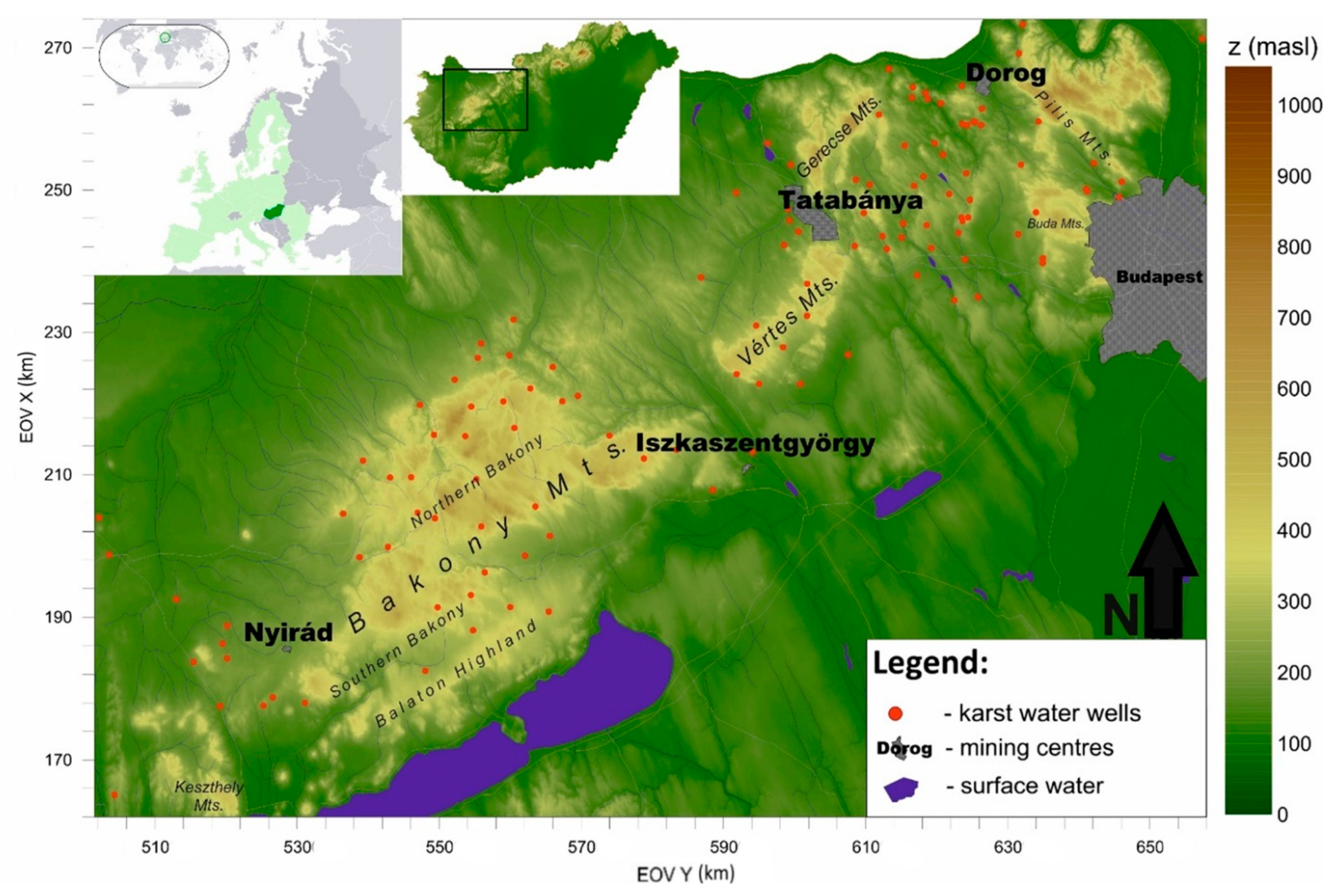
2.1. Hydrogeological Description of the Study Area

The Transdanubian Range is located in the mid-western part of Hungary (Figure 1). The extension of its karst system is approximately $300\times 100$ km [30], composed mainly of Mesozoic formations lying on slightly metamorphosed Paleozoic formations. The most significant of these are the aquifers forming a continuous hydraulic system of the Upper Triassic Main Dolomite and the Dachstein Limestone Formations, with a total thickness of 1.5–2 km [36]. In some areas of the Transdanubian Mountains, above the thick Triassic aquifer, there are locally occurring Jurassic-Cretaceous (Tata Limestone Fm, Zirc Limestone Fm, Ugod Limestone Fm) and Eocene (Szőc Limestone Fm) carbonates forming a hydraulically connected unit with the older formations. The aquitard formations (with lower hydraulic conductivity) located between the aquifers of different ages have the vertical flow slowed down, but they do not prevent it completely [37]. The pre-Cainozoic structure of the Transdanubian Range Unit can be characterized as mainly due to SW-NE compression. As a result, a syncline structure was formed in the middle of the Cretaceous, characterizing the geological settings of the area with the deformation of previously deposited sediments [38].

In the Late Cretaceous, karstification began in the Upper Triassic formations outcropping at the edge of the syncline. Therefore, bauxite deposits were formed in several places in the Northern Bakony Mts. and the Western part of the Southern Bakony Mts. [39,40]. As a result of tectonic movements beginning in the Late Eocene, so-called Paleogene Basins were formed along lateral displacements [41]. Along the indented coastline, the environment was also favorable to the formation of the Eocene bauxite [42].

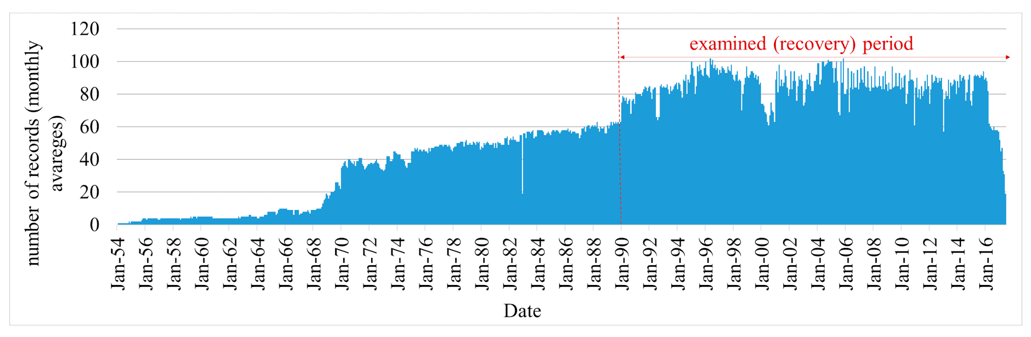
2.2. Dataset Description

The karst water monitoring network of the Transdanubian Range, established in the early 1970s, has since provided a large amount of information on the status of groundwater changes. The karst water level time series for which trend analysis performed in this study originate in the monitoring wells (Figure 1) of four Hungarian water directorates, and basically include data from the establishment of these up to 2016 or 2017. After preliminary screening, 107 time-series were found to bear witness to the recovery process of the karst system, a process characterized by rising water levels. In more than a third of these (40 wells), data were only available from 1990 or later, and there were several cases (12 wells) in which monitoring ceased in 2010 or before. Water level measurements were not equidistant in time. Regarding the recovery period (1990–2017), 31,438 monthly averages were examined for 107 wells, of which 4113 cases out of the ca 32,000 monthly average water level data (13% of months) had no measurements. Missing data were mostly from the early 2000s (Figure 2).

Monthly precipitation data were gathered from 47 precipitation monitoring stations and 5 climate stations in the area.

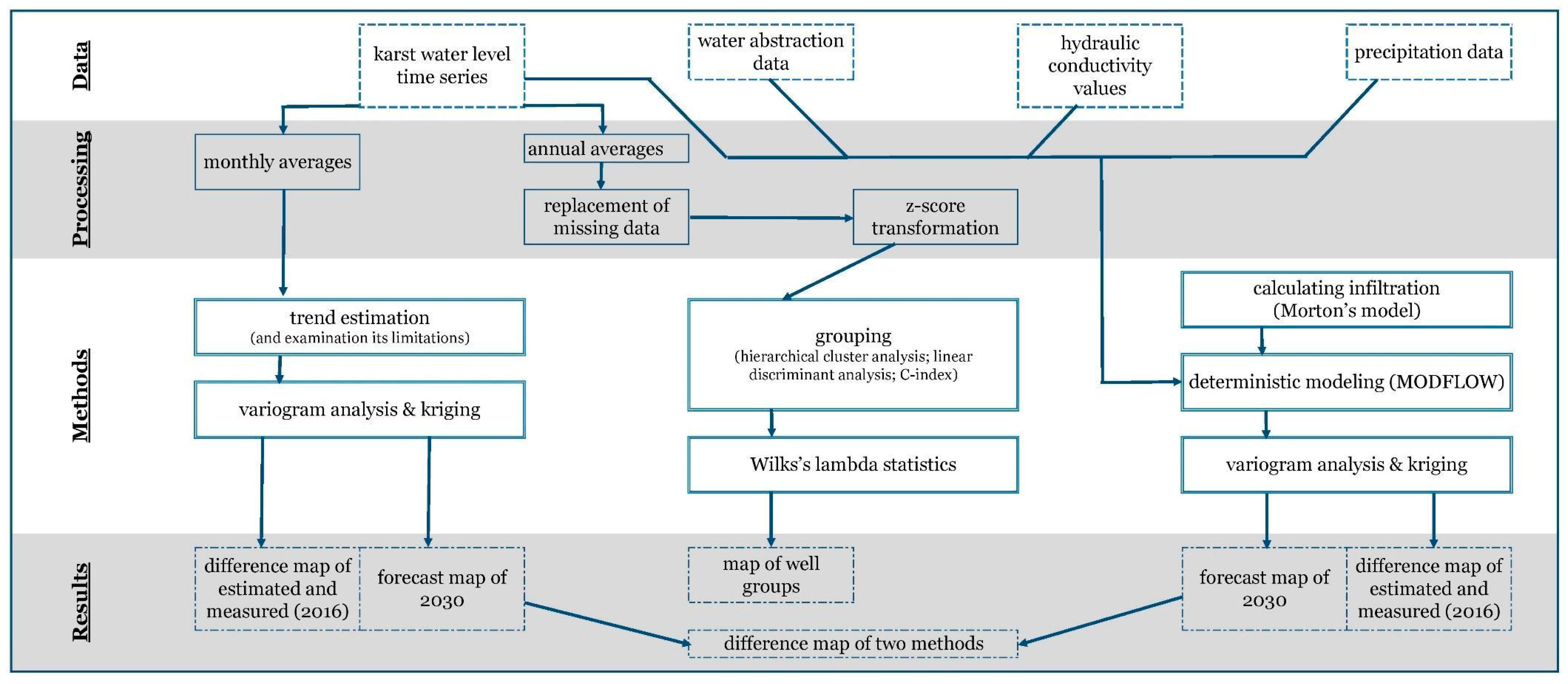
2.3. Applied Methodology

In order to examine the karst water recharge of the karst system in the Transdanubian Range, the following steps were followed (Figure 3).

To meet the aims of the study, after preprocessing the karst water levels (outlier removal etc.) and choosing the focus period of the research (1990–2017) (Section 1.2), the karst water monitoring wells were grouped using cluster analysis [43] on the basis of their annual average karst water levels. The groupings were then validated using linear discriminant analysis [44] and C-index [45] (Section 2.4), as in other studies dealing with subsurface water [46,47]. The years most important in driving the groupings were determined using Wilks’ λ statistics [48]. These steps follow the procedure presented in Hatvani et al. [44].

Monthly average karst water data were used for trend estimation, which was achieved by fitting growth models (Section 2.5). After choosing the model, which best described the recovery process, karst water levels were predicted in each well for January 2030.

The karst water levels were also predicted using deterministic modeling (Section 2.6). For this, the infiltration rate was calculated from precipitation data. The average annual recharge rate was calculated in the infiltration areas of the reservoir on the basis of hydraulic model tests performed in recent decades. The initial hydraulic conductivity values used in the early stages of model calibration were derived from pumping test data and literature. The final calibration of the deterministic model was performed using a dataset consisting of the 107 well data—the subject of the study—extended with historic water levels from additional ~100 subsurface wells and 60 springs. These not necessarily spanned the same time interval neither with each other nor with the 107 wells. Because these data were either gappy or covered a too short time period, these could not have been used for purposes other than the calibration of the deterministic model in the study. The database of the model also contains the monthly production data for karst wells, rising shafts, and all of the other water abstraction sites. After running the deterministic model, karst water levels were predicted for January 2030.

For the karst water values forecast by trend estimation and deterministic modeling, variogram analysis was applied [49] to interpolate (krige [50]) the water levels in 2016 and 2030 (Section 2.7). The predicted values of the two methods were then compared on difference maps.

2.4. Cluster and Discriminant Analysis

Cluster analysis aims to group observations (in this case, monitoring wells) on the basis of measured data (here, annual average water level time series)—in which those with similar properties (patterns) are placed in the same group (cluster). To achieve this, Ward’s [43] hierarchical classification method with squared Euclidean distance was applied to the Z-score transformed data. On account of missing data, the process of grouping could only be performed for 94 time series from 1995 to 2015. In order to obtain maximal separation between groups and simultaneously minimize variability within them, Fisher’s linear discriminant analysis (LDA) was used in the transformations (i.e., linear combinations) of the original data [44]. The grouping was also validated with the use of the C-index [45], which is regarded as being among the six best indices of correct cluster recovery [40].

In order to define which parameter plays the greatest role in determining the formations of the cluster groups, Wilks’s lambda (λ) [48] quotient was used. The value of λ is the ratio of the within-group sum of squares to the total sum of squares and is a number between 0 and 1. If λ = 1, the role played by that parameter in the grouping is the same in every case, and there is, therefore, no inter-group variability. Thus, that particular parameter did not affect the composition of the cluster groups [44,51,52]. If, on the other hand, λ = 0, the parameter under consideration affected the formation of cluster groups to the greatest degree. Therefore, one can say that the smaller the quotient, the greater the degree to which it determines the formation of the various cluster groups.

2.5. Trend Estimation

2.5.1. Growth Curves

Growth curves in general can be characterized by an upper limit (expected maximum value). Out of the 10 different type of curves used, one type of them does not have an inflection point and have a concave run in the domain of 0–∞. Three of this type of function were used in the study: Bertalanffy [53], Törnquist1, and Törnquist2 [54,55]. For additional technical specifications on the applied curves see the Supplementary Material Section S1.

There are processes that display an exponential rise initially, but over time, the growth slows down. This type of growth curves has an inflection point and they are also called sigmoid curve [56]. Relative to the inflection point, the initial section is concave, while the section after that is convex. The inflection point indicates that there have been some significant changes in the process. This type of curve is the original logistic function, but there are a number of mathematical functions with a similar shape. In this research, seven of these functions were examined, namely, the logistic function [57], the delayed logistic function [58], the squared logistic function [59], the Gompertz function [60], the “63 percent” trend function [58,59], the Johnson function [61], and the Richards function [62]. The main difference between these functions is to be found in the position of the inflection point, and in the shape of the curve. In the case of the Richards function, an additional v parameter was incorporated into the model, with which the location of the inflection point can be controlled.

2.5.2. Model Fitting

As a first step in the estimation of the functions, the expected maximum water level value (K)—prior to the beginning of intensive dewatering in 1950 [63]—of each well was determined and inserted into the calculation. Estimating the trend requires water level time series of appropriate quality and length, which is an obvious limitation. However, the most specific prerequisite is the maximum water level (K value). The water levels vary depending on the parameters characterizing the aquifer, so they characterize the hydrogeological environment of the observation. No additional parameters (e.g., infiltration and hydraulic conductivity) are required for this method.

In not every case is information available on the maximum water levels, prior to the mining activities, i.e., dewatering. In the present case, these figures were, in fact, available. In should be noted, that if not available, the trend estimation procedure can provide a rough estimate for the K value(s) as well by minimizing the error, which in some cases results in an overestimation of the value (Supplementary Material Table S3). Since the K value is the primary requirement and limitation of the method, it was examined whether its deviation within a certain range affects the goodness of fit or not. It was observed that the K value thus obtained is not realistic in all cases. However, the predicted water level did not deviate significantly.

Subsequently, the karst water level values were predicted for each examined well with the best fitting model of the trend analysis. Curved regression was performed using the least square method, with the best fit being determined on the basis of the maximized r² value, in the present case called “correlation index” determined by Kenney and Keeping [64] (Equation (1)), which is not similar to the frequently used Pearson or Spearman correlation coefficient. It takes into account the spread of the modelled values by standardizing the squared error of the prediction (SSE) with the sum of squares total (SST) (see Equation (1)). In other words, the smallest the SSE, the closer r² will get to 1. The best fit was found with changing each parameter iteratively to maximize the r² value.

The r² was calculated based on this function (Equation (1)):

$$r^2=1-\frac{{{\displaystyle \sum }}_t{\left(y_t-{\widehat{y}}_t\right)}^2}{{{\displaystyle \sum }}_t{\left(y_t-{\overline{y}}_t\right)}^2}=1-\frac{SSE}{SST},$$

(1)

where SSE = sum of squared errors; SST = sum of squares total.

The question of which model performs the best under different degree of missing data, i.e., measured values from the beginning of the time series were deleted yearly (maximum 5 years), was investigated experimentally. After that, the function fitting was re-performed. For this purpose, the 53 time series clearly displaying the exact beginning of the recharge period were used. This means that data were available for dates before 1990.

2.6. Deterministic Model

The deterministic model describing the recovery of the Transdanubian Range is a transient (not steady-state) hydraulic model (Supplementary Material Section S2). The model area is divided up into a constant orthogonal grid, the size being $500\times 500$ m for the total model area. The upper 200 m of the karst aquifer was built into the model. The unit of time in the transient model is 1 month. In areas where leakage is possible between the Triassic and overlying aquifers (e.g., Cretaceous limestones, Upper Pannonian porous layers), the model calculates the water exchange between the two aquifers on the basis of hydraulic conductivity. The flow rate between the karst aquifer and surface waters was also calculated using the hydraulic model.

The model also includes the major karst springs, which are regarded as fixed drains in the model. In every such location, the flow of the spring is modelled based on the difference of the calculated karst water level and the elevation of the spring multiplied by the localized conductivity value. On the basis of the difference between the karst water level and the elevation of springs, their discharge can be calculated. The recharge is equal to the spatial characteristic of diffuse infiltration, which can be determined from the product of the open karstic infiltration and its intensity. In the calculation of the latter, data from rainfall measuring stations close to the infiltration areas were used. In Hungary in karstic areas surface runoff is negligible, precipitation is instrumentally measured, thus using the base-function of hydrology seepage can be determined by subtracting evapotranspiration—estimated using the Morton CRAE model [65]—from precipitation. Monthly karst water abstraction data were included in the model, as well.

The results of modeling in general, including deterministic modeling, strongly depend on the uncertainty of the input parameters, let them be measured (e.g., yield) or calculated (e.g., infiltration). Using station data, gridded values have to be estimated, which again is highly dependent on the number and spatial distribution of the measured data. Furthermore, the result of the deterministic modelling was also significantly dependent on the exploration of the study area, i.e., on the (hydro)geological information. Thanks to the previous research, the Transdanubian Range was well explored as a result of which a relatively large amount of data is available.

The regionally updated database of the model allows the simulation of water level changes, discharge changes of major karst springs in the karst reservoir from 1951 up to the present day. Furthermore, it is also suitable for predicting changes in the expected karst water level.

2.7. Variography and Interpolation

As a final product, two forecast maps were made for January 2030 based on the water levels predicted by trend estimation and deterministic modeling. For the creation of the maps, the kriging of an “optimal” interpolation is necessary, and this is then be employed in the study to estimate the covariances to the highest degree of accuracy possible before mapping [50,51]. To obtain the weights for kriging, theoretical semivariograms are derived describing the spatial autocorrelation structure of the data by minimizing the variance of the error [66]. One of the most common theoretical models is a spherical model, which displays a linear behavior at the origin and the sill is reached at a, while a Gaussian model has a repressed slope (a tangent with zero slope at the origin), and its sill is a limited value that might be approximated to an infinitesimal degree, but never reached. Thus, in the case of the Gaussian model, a practical and an effective range a_e = a × √3 have to be determined; a_e is then used for further geostatistical modeling. A theoretical model can be given by calculating the empirical semivariogram using the algorithm of Matheron [67] (Equation (2))

$$\gamma \left(h\right)=\frac{1}{2N\left(h\right)}{\displaystyle \sum }_{i=1}^{N\left(h\right)}{[Z\left(x_i\right)-Z\left(x_i+h\right)]}^2,$$

(2)

where $\gamma \left(h\right)$ is the semivariogram and $Z\left(x\right)$ and $Z\left(x+h\right)$ are the values of a parameter sampled at a planar distance $\left|h\right|$ from each other, N(h) is the number of lag-h differences, i.e., $n\times \left(n-1\right)/2$ and n corresponds to the number of sampling locations at a distance h. The most important properties of the semivariogram used in the present study are the nugget, which quantifies the variance at the sampling location (including information regarding the error of the sampling), the sill, that is, the level at which the variogram stabilizes, which is the sum of the nugget (c₀) and the reduced sill (c), and the range (a), which is the distance within which the samples have an influence on each other and beyond which they are uncorrelated [68,69]. If the semivariogram does not have a rising part and the points of the empirical semivariogram align parallel to the abscissa, a nugget-type variogram is obtained. In this case, the sampling frequency is insufficient to estimate the sampling range using variography [50,70].

2.8. Used Software

Data preprocessing was performed in Microsoft Excel 16.0. IBM SPSS 22 was used for the cluster, Wilks’ λ, and discriminant analyses, and deterministic modeling was carried out in Applied Visual MODFLOW. The geostatistical modeling was performed in GS+ 10 and the mapping in Golden Software Surfer 15.

3. Results

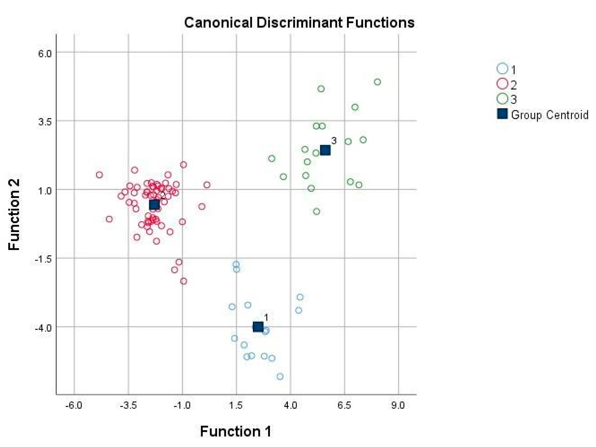
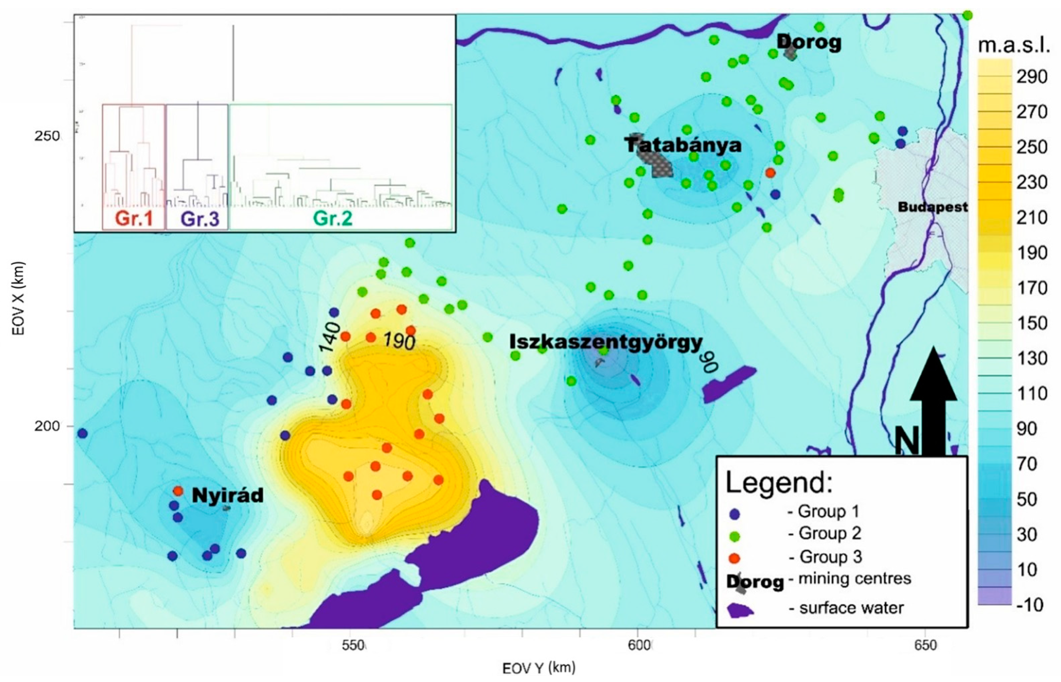
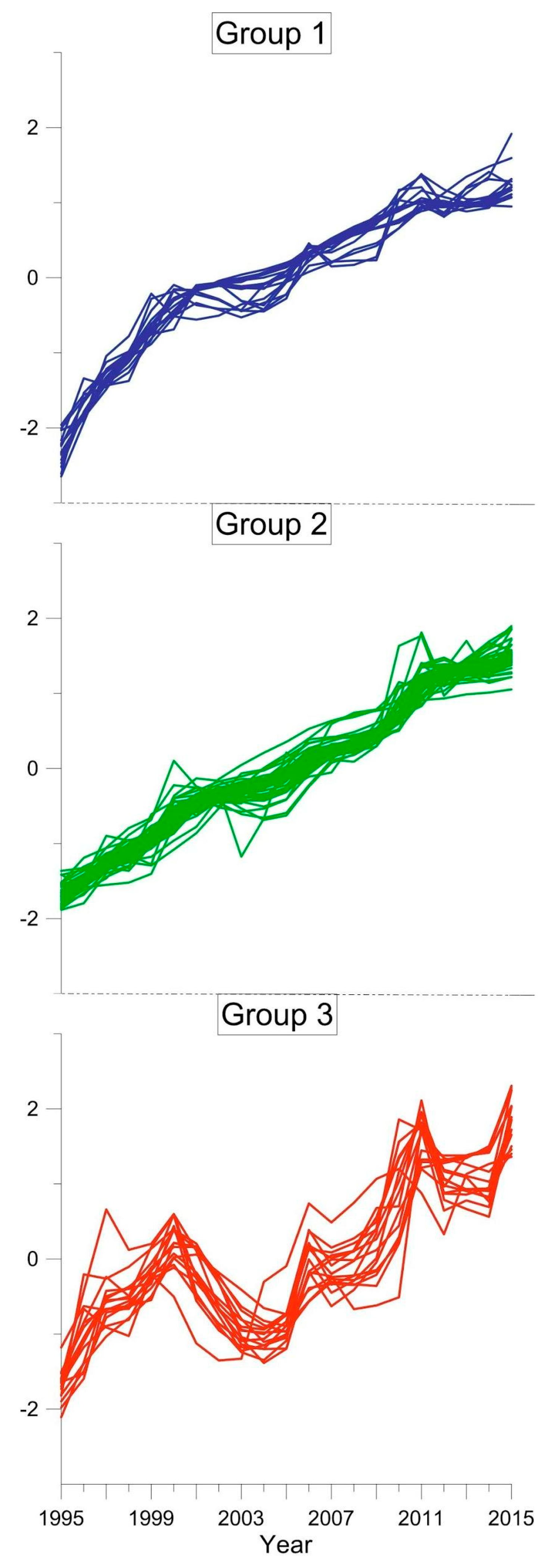
3.1. Cluster Analysis

Three groups of the 94 examined time series could be distinguished for the period 1995–2015. The grouping was 100% successful according to the linear discriminant analysis and can be well illustrated using the LD1 and LD2 functions (Figure 4 and Figure 5).

The value of the C-index was also calculated in the cases in which there are 2–10 groups, on the basis of which it can be determined that three is the optimal group number (the C-index is the smallest in this case).

Based on the 21 years examined in this study, the values of the Wilks’ λ quotient are higher on average in the first part of the period and lower in the second part. Thus, the initial phase of the time series was predominant in the spatial separation of the groups.

The three groups are also separated spatially (Figure 5). The 17 wells of the first cluster are located in the SW part of the Transdanubian Range, in the vicinity of the Nyirád mining center. These time series are characterized by a constant rising tendency and a minimal fluctuation pattern. The initial phase (ca. 1995–1999) of the recovery was faster than the following period (Figure 5). The second group contains 60 wells, which are situated in the NE part of the area, in the vicinity of the Dorog, Tatabánya, and Iszakszentgyörgy mining centers. The time series of this group are characterized by a constant increase at a similar rate throughout the examined period, with a minimal fluctuation pattern. The 17 wells of the third group are located in the western part of the Bakony Mts., which is a recharge area. Here, the karst water levels are higher (even at the beginning of the 1990s, the figure was about 290 m asl.) compared to the surrounding areas.

3.2. Trend Estimation

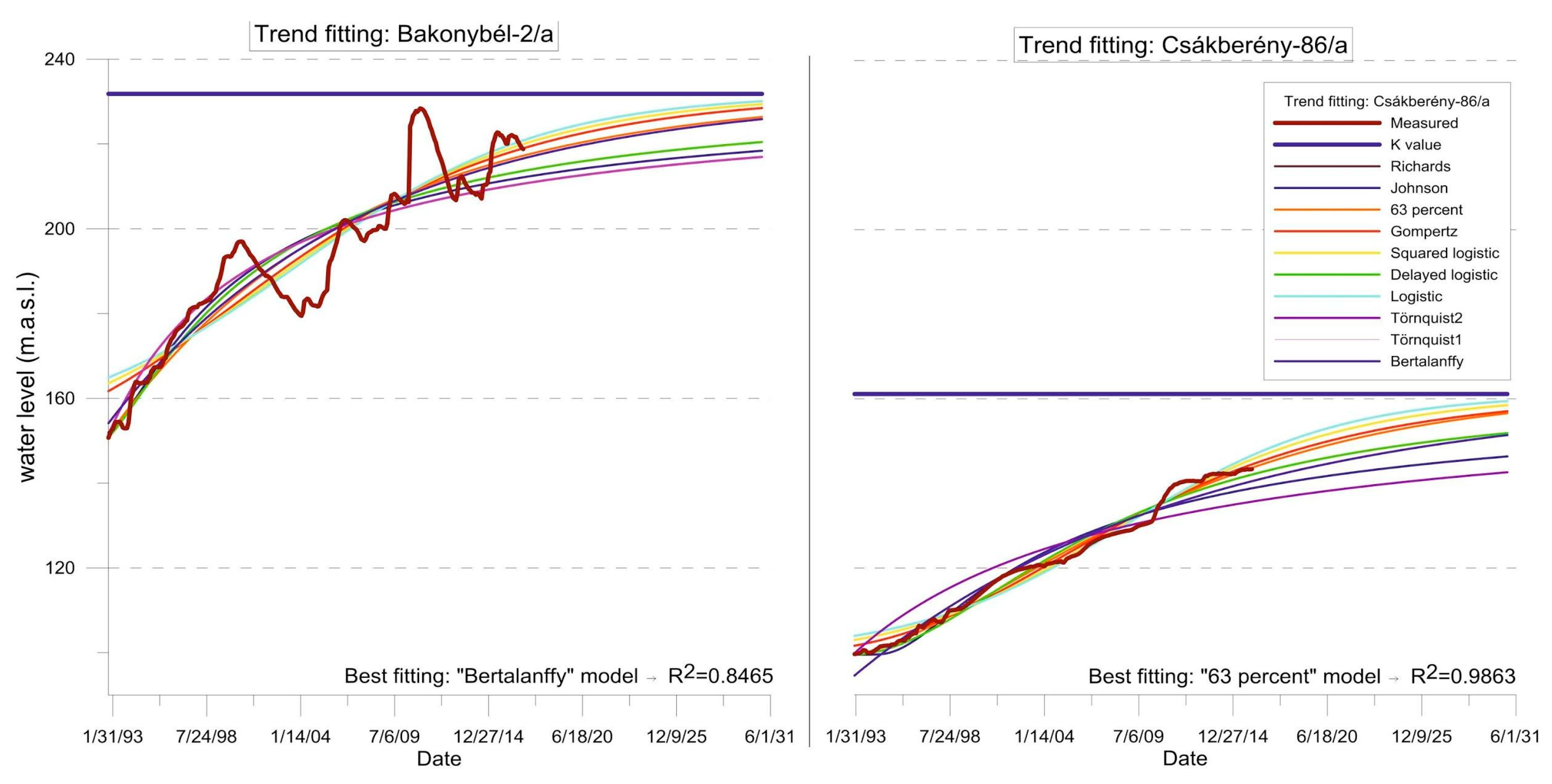
3.2.1. Determining the Best-Fitting Model

The various functions presented previously (Section 2.5) were fitted to the monthly average karst water time series. In order to carry out the trend fitting even under the condition ${\widehat{y}}_0=0$, the trend function was fitted not to the absolute water levels, but to the values of water level change relative to the beginning of the recovery phase, e.g., Figure 6.

Based on a two-tailed T test, all model runs were significant at p = 0.05. In most cases (82.24%), the curves showed a very good fit (r² > 0.9). However, it could be established that there is not a single function among those examined that best describes the recovery process in the Transdanubian Range. In most cases, the Richards (29.91% of cases) model proved to be the most accurate. However, the accuracy of the fitting—that is, the value of r²—showed very little difference between the functions in several cases. Because the value of r² can be similarly high in the case of different functions, the question of which functions fit best was addressed, taking into consideration not only the case with the largest r² value, but all of the cases in which $r^2\ge r_{max}^2-0.005$ (

Table 1. Number of best fits in the case of the different models for the 107 wells, based on the highest r² value (top row) and based on the cases in which the values of $r^2\ge r_{max}^2-0.005$ (bottom row).

		Bertalanffy	Törnquist1	Törnquist2	Logistic	Delayed Log
r2 = max.	%	11.21%	0.00%	1.87%	1.87%	17.76%
r2 ≥ (max.—0.005)	%	32.71%	3.74%	6.54%	20.56%	33.64%
		Squared log	Gompertz	63 percent	Johnson	Richards
r2 = max.	%	0.00%	4.67%	28.04%	4.67%	29.91%
r2 ≥ (max.—0.005)	%	22.43%	31.78%	48.60%	17.76%	52.34%

). However, even despite this, the Richards model proved to be the functions describing the recovery process the best. It should be noted that the difference between the goodness of fits (r² values) obtained for the different functions was quite small.

3.2.2. Limitations of Trend Estimation

In some measured time series, data for the first few years of the recovery are missing. However, these also show the character of the recovery phenomenon and contain valuable information about it. It was necessary to examine to what extent the goodness of fit and the accuracy of the predicted water levels are affected even if a few years of the measured data are missing from the beginning of the time series. On the basis of the examination of 53 wells, it was found that only a few missing data (a 1-year gap in 24.53% of cases) cause little difference. However, as the amount of missing data increases, this causes more differences (a 5-year deficit in 77.55% of cases) over the issue of which function fits best (

Table 2. Number and rate of change of the best fitting function in the case of 1–5 years of missing data.

Missing Year(s)	1	2	3	4	5
Number of changed time series	13	26	28	35	38
Percent of changed time series	24.53%	49.06%	52.83%	66.04%	77.55%

).

The example of five randomly selected time series illustrates how r² and the water level values predicted for January 2030 would change if a longer period was missing from the beginning of the recovery time series. The aim was to rank the functions in the case of 1–5 years of missing data compared to the case of time series with no missing data (

Table 3. Changes in r² values and water levels predicted for January 2030 in case of 1–5 years of data missing from the beginning of the time series, in the case of 5 wells representing the different parts of the whole study area.

Well		Number of Missing Year(s)
		0	1	2	3	4	5
Bakonybél-2a	Best fitting function	Bertalanffy	Squared log	Richards
	max. r2	0.85	0.82	0.80	0.78	0.76	0.74
	January 2030 (m asl.)	225.5	228.9	230.6	231.1	231.1	231.1
	deviation in forecast (%)	0.00%	1.52%	2.27%	2.47%	2.51%	2.49%
Csákberény-86a	Best fitting function	“63 percent”			Gompertz	Richards
	max. r2	0.99	0.98	0.98	0.98	0.98	0.97
	January 2030 (m asl.)	156.1	155.6	155.7	155.4	157.1	157.9
	forecast deviation (%)	0.00%	0.32%	0.31%	0.50%	0.62%	1.11%
Duka-1	Best fitting function	Delayed log
	max. r2	0.99	0.99	0.99	0.99	0.99	0.98
	January 2030 (m asl.)	171.5	171.0	171.5	171.3	170.6	170.7
	forecast deviation (%)	0.00%	0.29%	0.04%	0.12%	0.50%	0.45%
Epöl-5	Best fitting function	“63 percent”
	max. r2	0.99	0.99	0.99	0.99	0.99	0.98
	January 2030 (m asl.)	134.8	134.0	134.7	134.0	134.0	134.6
	forecast deviation (%)	0.00%	0.57%	0.07%	0.61%	0.62%	0.17%
Tata-Pokol	Best fitting function	“63 percent”					Gompertz
	max. r2	0.99	0.99	0.98	0.98	0.98	0.97
	January 2030 (m asl.)	146.8	147.4	147.4	147.0	147.0	149.9
	forecast deviation (%)	0.00%	0.38%	0.43%	0.13%	0.14%	2.08%

). Although the best-fitting function does indeed change in many cases for the five randomly selected wells, there was no remarkable change in the estimated values. In the case of 5 years of missing data, the largest change in the predicted water level occurred at the Bakonybél-2a well, where the deviation is about 2.5% compared to the prediction based on the whole recovery time series. It is also noticeable that the time series of Bakonybél-2a are characterized by significant, long-term water level fluctuations (Figure 7).

Another important element of the method employed is the determination of the threshold value, which the water level asymptotically approaches. This can be specified before the fitting, on the basis of the user’s a priori knowledge. Many observation wells were established only after the beginning of dewatering, in the early 1970s, so the undisturbed water levels in the pre-mining period were not always precisely known. An experiment was performed in which the K values of five randomly selected wells were reduced and increased by 2% repeatedly, until they had reached ± 10%, compared to the value originally determined (

Table 4. Changes in r² values and water levels predicted for January 2030 in the case of modifying the threshold value by max. +/− 10%, in the case of 5 wells representing the different parts of the whole study area.

Well		Percentage of Original K Value
		90%	92%	94%	96%	98%	100%	102%	104%	106%	108%	110%
Bakonybél-2a	Best fitting function	Bertalanffy
	max. r2	0.84	0.84	0.84	0.84	0.85	0.85	0.85	0.85	0.85	0.85	0.85
	January 2030 (m asl.)	220.6	221.7	222.7	223.7	224.6	225.5	226.3	227.1	227.9	228.6	229.3
	forecast dev. (%)	2.15%	1.68%	1.23%	0.80%	0.39%	0.00%	0.37%	0.73%	1.07%	1.40%	1.71%
Csákberény-86a	Best fitting function	“63 percent’
	max. r2	0.98	0.98	0.99	0.99	0.99	0.99	0.99	0.99	0.99	0.99	0.99
	January 2030 (m asl.)	152.7	153.4	154.2	154.9	155.5	156.1	156.7	157.3	157.8	158.3	158.8
	forecast dev. (%)	2.23%	1.73%	1.27%	0.82%	0.40%	0.00%	0.38%	0.74%	1.08%	1.41%	1.72%
Duka-1	Best fitting function	“63 percent”		Bertalanffy	Delayed lg
	max. r2	0.99	0.99	0.99	0.99	0.99	0.99	0.99	0.99	0.99	0.99	0.99
	January 2030 (m asl.)	168.3	169.9	171.2	169.6	170.6	171.5	172.3	173.1	173.8	174.5	175.1
	forecast dev. (%)	1.86%	0.94%	0.15%	1.08%	0.52%	0.00%	0.48%	0.93%	1.36%	1.75%	2.12%
Epöl-5	Best fitting function	“63 percent”										Bertalanffy
	max. r2	0.9895	0.9899	0.9902	0.9905	0.9907	0.9909	0.9911	0.9912	0.9914	0.9915	0.9916
	January 2030 (m asl.)	133.35	133.69	134.00	134.29	134.56	134.82	135.06	135.28	135.49	135.68	135.78
	forecast dev. (%)	1.09%	0.84%	0.61%	0.39%	0.19%	0.00%	0.18%	0.34%	0.50%	0.64%	0.72%
Tata-Pokol	Best fitting function	“63 percent”
	max. r2	0.9841	0.9846	0.9851	0.9855	0.9858	0.9861	0.9863	0.9866	0.9868	0.9869	0.9871
	January 2030 (m asl.)	144.56	145.07	145.55	146.00	146.42	146.81	147.17	147.52	147.84	148.14	148.43
	forecast dev. (%)	1.53%	1.18%	0.86%	0.55%	0.27%	0.00%	0.25%	0.48%	0.70%	0.91%	1.10%

). It was established that the greater the degree of the change in the K value, the greater the variety of the type of functions which gave a best fit. Furthermore, it was established that the water levels predicted for January 2030 showed only a few meters’ difference even in the case of a relatively high degree of inaccuracy in determining the K maximum value. The analysis of the five time series demonstrates that the greatest deviation from the water levels originally estimated for January 2030 is 2.15%, as also observed at the Bakonybél-2a well, which has a definite fluctuation pattern.

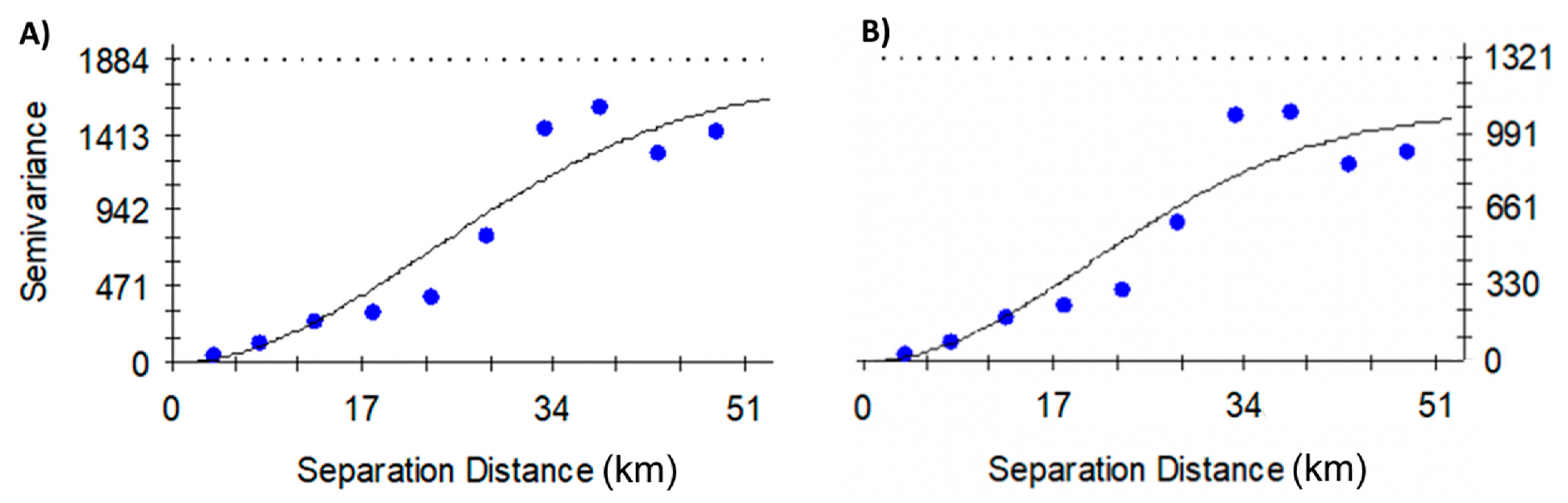
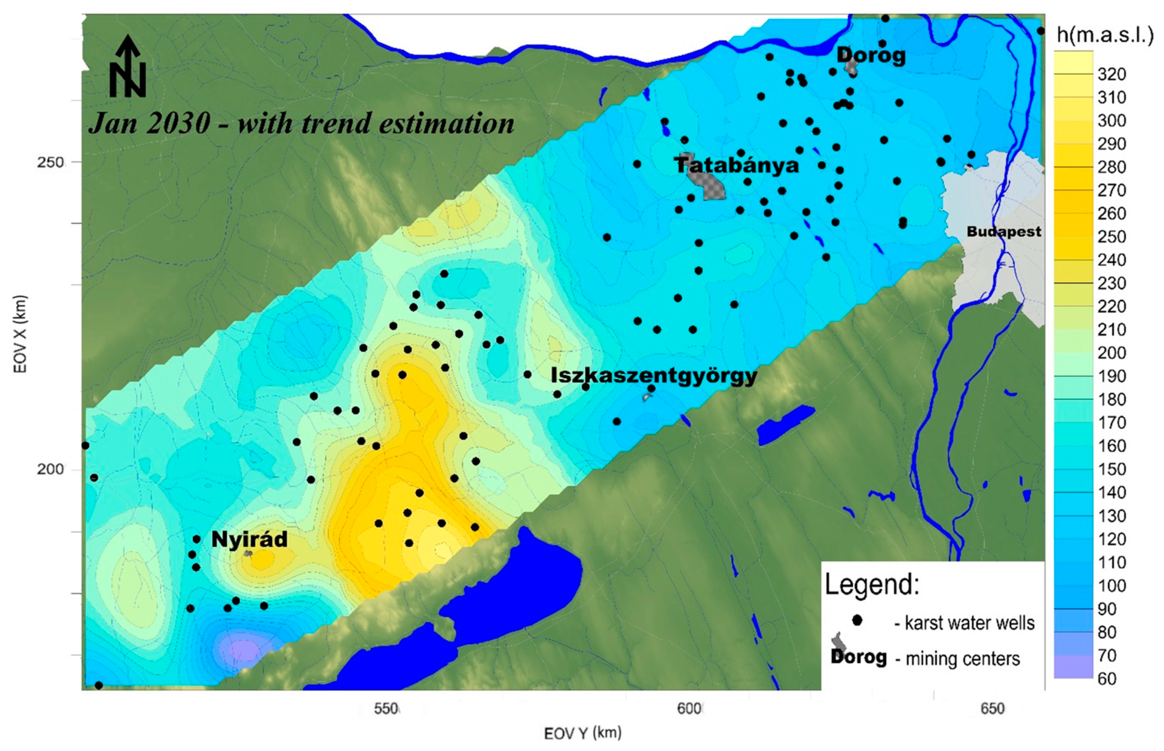
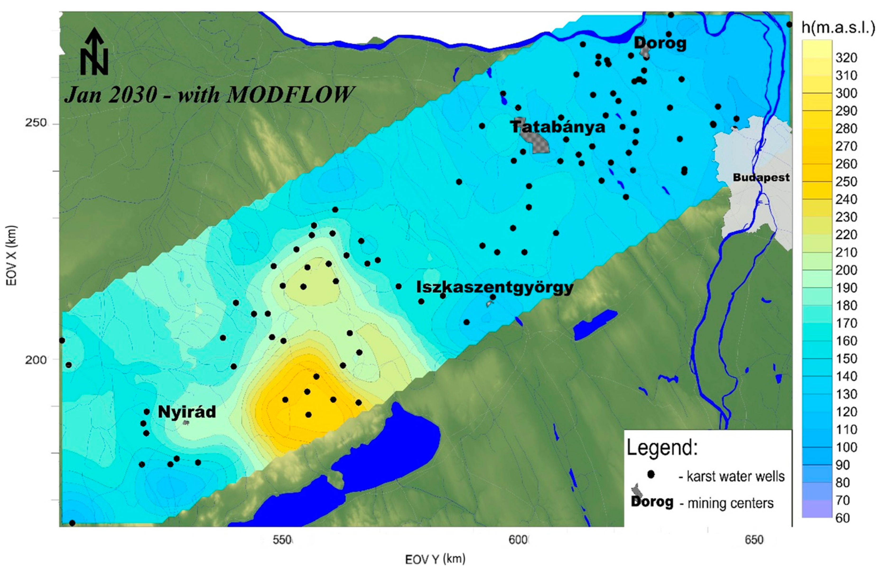
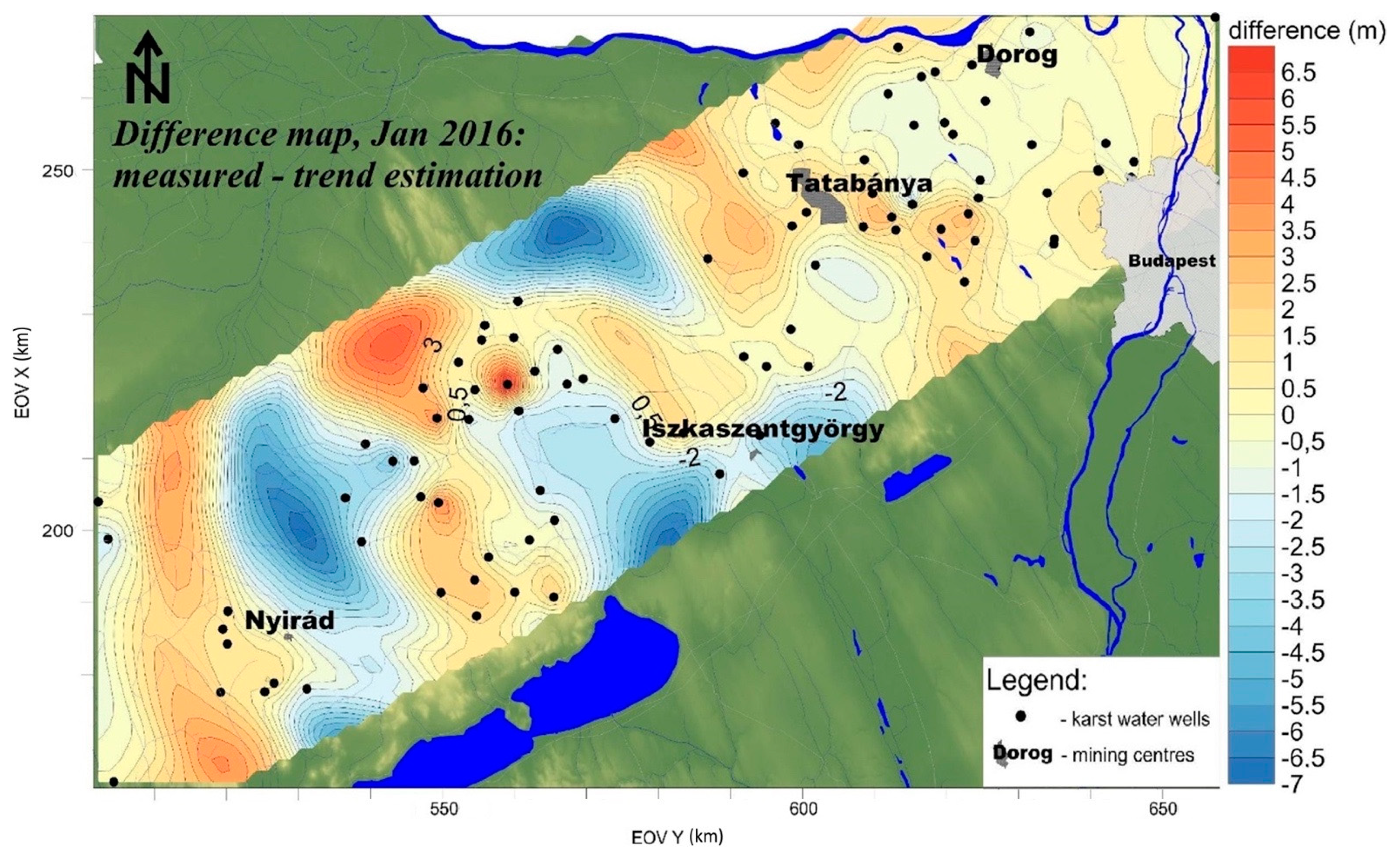
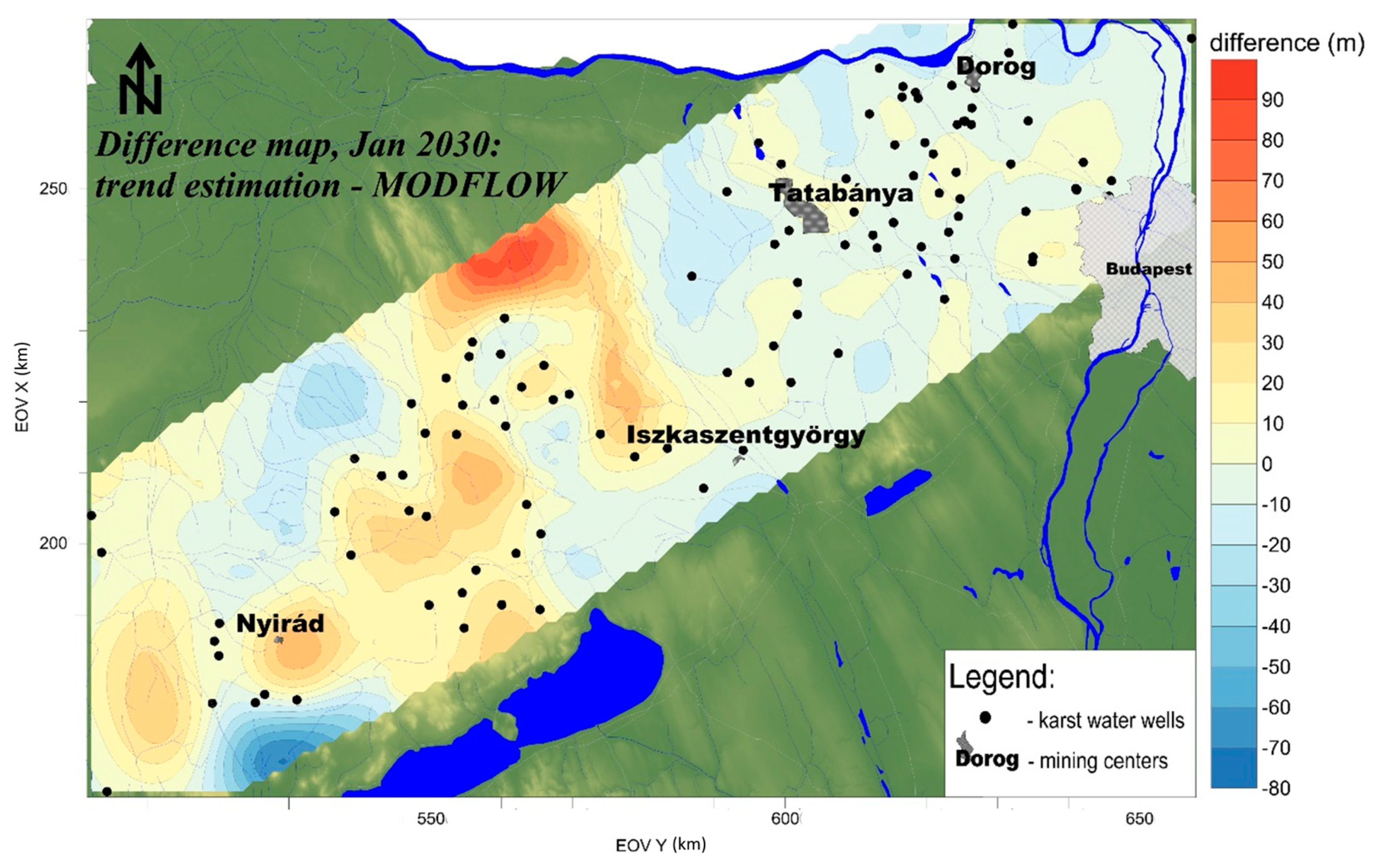
3.3. Variography and Predicted Karst Water Level Maps

Water levels were forecasted using two methods: the extrapolation of the best-fitting trend in each well and the construction of a deterministic model. To assess whether the predicted water levels have a spatial autocorrelation structure, empirical semivariograms were estimated, and these indicated a similar, nested structure. Based on the values obtained by trend estimation, a 32.5 km range stood out, while in the results of the modeling, this was true of the spatial ranges of 18 and 39 km (Figure 8).

For better illustration, 2D surfaces were modelled with kriging from the predicted values for each observation point based on the two methods. According to the map prepared on the basis of the trend estimation (Figure 9), the highest water levels can be expected in the central-SW part of the Transdanubian Range, in the central areas of the Bakony Mts., where the highest water levels are predicted to be in 2030 between 280 and 310 m asl. Low water levels are still expected around mining centers, but a clearly demarcated depression area can no longer be identified. The lowest water levels are expected at the SW (~65 m asl.) and NE (95–115 m asl.) edges of the area.

Based on the values of the deterministic modeling, the map of January 2030 (Figure 10) forecasts slightly lower water levels compared to the other method. The highest predicted water levels can also be expected in the Bakony Mts. according to this approach, with water levels slightly higher than 270 m asl, while the lowest predicted water levels in the edge of the area are between 110 and 120 m asl.

In order to examine the accuracy of the estimation by trend fitting, a difference map between the measured and estimated water levels was prepared for the beginning of 2016 (Figure 11). The maximum deviation between the estimated and measured values is about 8 m, while the median of the deviations is approximately 1 m, hence the difference between the measured and estimated values is below 1 m in at least half of the wells.

The difference between the values measured and those estimated using the deterministic model for January 2016 was also plotted (Figure 12). The maximum deviation is around 20 m for estimation by this method. The median of the differences is 3.29 m, so it can be concluded that the difference between the measured and estimated values exceeds this value in, at most, half of the wells.

Finally, the difference between the projections for January 2030 using the two different methods was examined. Therefore, a difference map based on the values calculated by trend estimation and deterministic modeling was prepared (Figure 13) in such a way that the results obtained by modeling were subtracted from the values obtained by trend analysis.

In some parts of the area shown on the map, where there are no monitoring wells, large differences can occur between the values estimated by the two methods; this, however, is a consequence of unreliable extrapolation. In areas where the amount of data is adequate on the basis of interpolation, the difference map shows the greatest differences in the central areas of the Bakony Mts. Here, the values estimated by trend analysis exceed the results of modeling, and in some places by as much as 30–40 m. In the NE part of the study area, on the other hand, the deterministic forecast gives higher expected water levels, but here, the difference between the results of the two methods is smaller (maximum 5–10 m). The median of the absolute deviations is approximately 4 m; thus, in at least half of the wells the difference between the values estimated by the two methods exceeds this value.

4. Discussion

When mining activity is ceased and dewatering is discontinued, a number of environmental problems emerge (e.g., [71]). Besides the general water quality deterioration of the subsurface water body, the large-scale change in groundwater levels over an extended area (e.g., [72,73,74]) pose an even higher threat to the generally vulnerable karstic areas. Such changes can cause extremely high hydraulic gradients favoring internal erosion and dissolution in the karst and changes in flow paths etc.; for an extensive review see Gutiérrez et al. [75].

After the collapse of the mining industry in the former Soviet Bloc [25,26] large-scale dewatering ceased in many former mining centers, causing an increase in water levels and the regeneration of the system. In Hungary, an extremely large amount of groundwater was abstracted from the karst aquifer of the Transdanubian Range for mining purposes between 1950 and 1990, as well. However, after the mine closure, the water level began to rise to an extreme degree in some areas (especially near to the mining centers) [27,30]. Thanks to the wealth of data from the monitoring wells in the area, water level changes can be examined extensively, the better to understand the recharge process and the behavior of the karst system.

Clustering groundwater time series is a common method to identify the individual behaviors of the different groups. Variant hydrochemical characterization [76,77] or hydrodynamic differences [78] can be determined by different types of cluster analysis—a method which is, furthermore, applicable to the task of revealing spatial separation. In the case of the Transdanubian range, the three groups of time series distinguished by cluster analysis are also spatially separated. The time series of this group also show a rising trend, but with a definite fluctuation pattern (Figure 14). As the grouping was based on the patterns, and not on the absolute value of water levels, the actual rate of the water level rise can also be very different for wells belonging to the same group. In the wells of the first group, the rise of the water level was between 3 and 58 m between 1995 and 2015. In the second group, the rise ranged from just a few meters to more than 100 m, while in the third group, it varied between 12 and 59 m. The grouping is influenced by the position of the wells associated with the different depression centers (Nyirád, Iszkaszentgyörgy, Tatabánya, and Dorog). This may be partly explained by the pattern of mine closures, which did not take place simultaneously, having given ever-greater impetus to the recovery of the reservoir. The first and the second cluster groups are not characterized by a definite fluctuation pattern, while in the wells of the third group located in the Bakony recharge area, further from the dewatering sites, the water levels show significant fluctuations. Thus, in addition to the recovery, the effect of infiltration is also significant in this area, a fact which is reflected in the time series. The Wilks’ λ quotient values obtained also indicate that the water level changes occur at a higher rate at the beginning of the recovery and gradually slow down towards the end of the process. Thus, the initial stage has the most significant effect on the pattern, and so therefore on the separation of the groups, as well.

What is certain is that significant groundwater increase on a regional scale can induce severe economic and technical-engineering issues [79]. In order to be properly prepared for these problems and to mitigate any damage, it is necessary to forecast the change in groundwater level as accurately as possible.

In most cases, groundwater level changes related to mining activity are modeled by numerical simulation, but this requires the simplification of a very complex system [80,81]. Rapantova et al. [82] studied the possibilities of deterministic modeling of groundwater flow in mining areas, and software with different approaches that can be used in different hydrogeological environments. They concluded that deterministic modeling can be the most suitable for answering certain, more complex hydrogeological questions (e.g., the assessment of the impact of hydraulic stresses) [82].

In karst aquifers, numerical simulation can be particularly complicated due to the peculiarities of such formations and, especially, the high degree of heterogeneity related to its triple porosity [80]. Furthermore, for modeling to be successful, a wide variety of input data are required, and these may be error prone or their calculation may give an uncertain result (e.g., in the case of infiltration) [83,84]. When it is a question of water level forecasting, several approaches can be expedient. Charou et al. [85] investigated water level changes due to the effects of mining by processing remote sensing data, which is an inexpensive and effective tool for indicating groundwater changes in mining areas. In order to obtain the most accurate water level estimation, it is recommended that the results obtained by different methods then be compared.

A special hydrogeological situation evolved as a result of mining activities in the Transdanubian Range, where the expected water levels can be estimated not only by deterministic modeling but also by trend analysis. Since the recovery process has an upper limit, functions with threshold values (growth curves) are best suited to describe its trend. From the 10 models examined, the Richards function proved to be the most suitable for describing the recovery process in the karst aquifer, supposedly to the underlying additional factor—compared to the other methods—that renders its computation flexible at the inflection point (Supplementary Material Section S1). The descriptive statistics of water level values predicted for 107 wells by 10 different methods for 2030 were also prepared (Table S4). The different models were compared based on the interquartile interval of their estimated values for 2030. The Richards function did not provide the smallest range. However, the interquartile range in the present case cannot be considered as a valid statistic to evaluate the goodness of the model predictions, because the now undisturbed and recovering karst water levels tend to follow topography (Figure. 1) [86,87], thus are expected to show a relatively high spatial variability in 2030. This variability is reflected in the relatively wider interquartile range of the “Richards” model (Table S4) and concurs with the “Richards” model giving the best fit regarding the correlation index (r²). This means that it was not only able to estimate the trend of the measured data but also its spatial variability among the wells.

The values estimated by trend analysis compared to the water levels measured for 2016 show a small difference in many wells; the median of these values is around 1 m. Considering that water levels in the karst systems may in any case be characterized by high temporal variability [80], this small difference in measured and estimated values confirm that the calculation using trend analysis gives an accurate result. The determination of the K threshold value is essential to this method; another requirement is that there be as many measured values from as long a time period as possible. The trend analysis and the forecasting with MODFLOW modeling give similar results, something which is supported by the similar variograms (with nearly identical ranges) that were obtained, as well as the similar spatial distribution of the water levels. The absolute difference in the water levels calculated for January 2030 by the two methods shows a difference of more than 4 m in at least half of the wells. The greatest differences occur in some of the wells in the south of the Bakony Mts, which is an infiltration area, so the time series here are characterized by relatively intense fluctuations. The difference may also occur because the two methods require fundamentally different input parameters. The calculation by trend analysis is based on the measured water level data, which already includes all the impacts affecting it. For MODFLOW modeling, several parameters (e.g., hydraulic conductivity, infiltration, yield of water abstractions) need to be provided, and any inaccuracy in these will affect the estimated values. Besides, during the construction of a deterministic model, a significant simplification of reality is inevitable, e.g., the aquifer of the Transdanubian Range was considered as continuous and a single layer. In the creation of a deterministic model, a more precise determination of leakage from the Cretaceous and younger cover layers is advisable.

Modeling is time consuming, requires a lot of input data (that is difficult to obtain and process), and can be erroneous. Trend estimation—especially for a lot of data—can also be time consuming, but it requires many fewer different datasets. The water level time series practically bear the imprint of all the effects on the aquifer; changes in the water level are the manifestation of all the effects. In addition, although a special case was examined in the present study, trend estimation as a water level forecast option can be applied to other areas of hydrogeology. In this particular case, the growth curves estimated the hydrogeological changes the most accurately. In other cases, it is also necessary to choose an appropriate trend function on the basis of the professional knowledge of the researcher so the water levels can be reliably predicted.

The more accurate forecast of groundwater level in such areas may become an urgent necessity. Using the methodology applied in this study, rises in groundwater can be examined in a reliable and easy-to-use way.

5. Conclusions and Outlook

The investigation of groundwater level rises and the prediction of water levels was presented and in which a novel methodology composed of different data analysis methods was applied to the former mining area of the Transdanubian Range. The time series of karst water monitoring wells in the Transdanubian Range were split into three groups by cluster analysis, and these groups may be spatially separated on the basis of their location relative to the depression centers, which are characterized by different patterns. Both the deterministic modeling (using MODFLOW) and trend estimation (using the Richards function out of all trialed ones) proved themselves suitable for forecasting of water level rises in the area for 2030. It should be noted, however, that their comparison reveals distinctive spatial differences in the predictions of the two methods. On the one hand, the results of modeling with MODFLOW were found to be greatly affected by the accuracy of the input parameters (infiltration, yields, geological model of the area, etc.) and how precisely the established conceptual model approximates reality. On the other hand, trend estimation with growth models provided similarly accurate results, but without the need for auxiliary data, simply through the investigation of the hydrographs, as they reveal the hydrogeological characteristics of their vicinity. Furthermore, based on the preliminary knowledge, it was necessary to specify the maximum water level as close as possible to the original undisturbed water level. It is possible to state this with some confidence, as neither the slight inaccuracy in specification of the maximum level, nor the few years of missing data at the beginning of the time series seems to affect the applicability of the growth models significantly.

Comparing the two methods, it can be stated that the application of growth curves in trend analysis can be more successfully applied in the forecasting of groundwater levels. The methodology applied to analyze the increasing groundwater level data can help to examine and forecast rising groundwater levels in many areas of the world characterized by such phenomena.

References

1. Coulson, M. The History of Mining: The Events, technology and people involved in the industry that forged the modern world; Illustrated edition; Harriman House: Hampshire, UK, 2012. [Google Scholar]
2. Brown, D.K. A History of Mining in Latin America: From the Colonial Era to the Present; University of New Mexico press: Albuquerque, NM, USA, 2012. [Google Scholar]
3. Kusuma, S. Environmental Impact Assessment of a Proposed Bauxite mining using Rapid Impact Assessment Matrix Method. Int. J. Appl. Environ. Sci. 2010, 5, 29–38. [Google Scholar]
4. Kamble, P.H.; Bhosale, S.M. Environmental Impact of Bauxite Mining: A Review. Int. J. Res. Appl. Sci. Eng. Technol. 2019, 7, 86–90. [Google Scholar] [CrossRef]
5. Cidu, R.; Biddau, R.; Fanfani, L. Impact of past mining activity on the quality of groundwater in SW Sardinia (Italy). J. Geochem. Explor. 2009, 100, 125–132. [Google Scholar] [CrossRef]
6. Howladar, M.F. Coal mining impacts on water environs around the Barapukuria coal mining area, Dinajpur, Bangladesh. Environ. Earth Sci. 2013, 70, 215–226. [Google Scholar] [CrossRef]
7. Jhariya, D.C.; Khan, R.; Thakur, G.S. Impact of Mining Activity on Water Resource: An Overview study. In Proceedings of the National Seminar on Recent Practices & Innovations in Mining Industry, Raipur, India, 19–20 February 2016; pp. 271–277. [Google Scholar]
8. Andrew, H.; Grigg, A.H. Hydrological response to bauxite mining and rehabilitation in the jarrah forest in south west Australia. J. Hydrol. Reg. Stud. 2017, 12, 150–164. [Google Scholar] [CrossRef]
9. Apaydın, A. Dual impact on the groundwater aquifer in the Kazan Plain (Ankara, Turkey): Sand–gravel mining and over-abstraction. Environ. Earth Sci. 2012, 65, 241–255. [Google Scholar] [CrossRef]
10. Huang, D.; Liu, Z.; Wang, W. Evaluating the Impaction of Coal Mining on Ordovician Karst Water through Statistical Methods. Water 2018, 10, 1409. [Google Scholar] [CrossRef] [Green Version]
11. Wu, Q.; Zhou, W.F.; Li, D. Management of karst water resources in mining area: Dewatering in mines and demand for water supply in the Dongshan Mine of Taiyuan, Shanxi Province, North China. Environ. Geol. 2006, 50, 1107–1117. [Google Scholar] [CrossRef]
12. Wu, Q.; Xing, L.T.; Ye, C.H.; Liu, Y.Z. The influences of coal mining on the large karst springs in North China. Env. Earth Sci. 2011, 64, 1513–1523. [Google Scholar] [CrossRef]
13. Li, G.; Zhou, W. Impact of karst water on coal mining in North China. Environ. Geol. 2006, 49, 449–457. [Google Scholar] [CrossRef]
14. Sherwood, J.M. Modelling Minewater Flow and Quality Changes after Coalfield Closure. Ph.D. Thesis, University of Newcastle, Newcastle upon Tyne, UK, 1997. [Google Scholar]
15. Sadler, P. Predicting groundwater recovery after mine closure. In Proceedings of the Mine, Water and Environment Congress, Sevilla, Spain, 13–17 September 1999; pp. 437–444. [Google Scholar]
16. Jin, W. Environmental geological hazards caused by abandoned mines and its prevention and control measures. Heilongjiang Sci. 2017, 20, 68–69. [Google Scholar]
17. Zhou, J. Risk analysis on adjacent mine water inrush caused by groundwater rebound of abandoned coal mine. Saf. Coal Mines 2013, 7, 166–168. [Google Scholar]
18. Wu, Q.; Wang, M.Y. Characterization of water bursting and discharge into underground mines with multi-layered groundwater flow systems in the North China coal basin. Hydrogeol. J. 2006, 14, 882–893. [Google Scholar] [CrossRef]
19. Toran, L.; Bradbury, K.R. Ground-Water Flow Model of Drawdown and Recovery Near an Underground Mine. Groundwater 1988, 26, 724–733. [Google Scholar] [CrossRef]
20. Younger, P.L.; Adams, R. Predicting Mine Water Rebound. Technical report; University of Newcastle: Newcastle upon Tyne, UK, 1999. [Google Scholar] [CrossRef]
21. Kim, S.-M.; Choi, Y. SIMPL: A Simplified Model-Based Program for the Analysis and Visualization of Groundwater Rebound in Abandoned Mines to Prevent Contamination of Water and Soils by Acid Mine Drainage. Int. J. Environ. Res. Public Health 2018, 15, 951. [Google Scholar] [CrossRef] [PubMed] [Green Version]
22. Dreybrodt, W. Processes in Karst Systems: Physics, Chemistry, and Geology, 1st ed.; Springer: Berlin/Heidelberg, Germany, 1988. [Google Scholar]
23. Ford, D.; Williams, P. Karst Hydrogeology and Geomorphology; John Wiley & Sons Ltd.: Chichester, UK, 2007. [Google Scholar]
24. Ellman, M. Socialist Planning; Cambridge University Press: Cambridge, UK, 1979; p. 17. [Google Scholar]
25. Crowley, S. Hot Coal, Cold Steel: Russian and Ukrainian Workers from the End of the Soviet Union to the Post-Communist Transformations; University of Michigan Press: Ann Arbor, MI, USA, 1997. [Google Scholar] [CrossRef]
26. Haney, M.; Shkaratan, M. Mine Closure and its Impact on the Community: Five Years after Mine Closure in Romania, Russia and Ukraine; Policy Research Working Paper No. 3083; World Bank: Washington, DC, USA, 2003; Available online: https://openknowledge.worldbank.org/handle/10986/18177 (accessed on 9 April 2021).
27. Nyírő, A. Tata: Collapse of the Karst Water System. Political and Economical Aspects of an Environmental Catastrophe in Hungary, 1950-2019. Studia Mundi Econ. 2020, 7, 52–58. [Google Scholar] [CrossRef]
28. Tóth, M. Mikor indulnak újra a tatai források? Vízügyi Közlemények 2002, 84, 195–209. [Google Scholar]
29. Körmendi, G. Tata-Tóváros, mint kedvelt fürdő- és üdülőhely (1773–1939). In A Vártól a Városig. Tata Évszázadai; Kisné Cseh, J., Ed.; Tata: Tata Város Önkormányzata, Hungary, 2004; pp. 233–253. [Google Scholar]
30. Alföldi, L.; Kapolyi, L. Bányászati Karsztvízszint-süllyesztés a Dunántúli-Középhegységben; MTA Földrajztudományi Kutatóintézet: Budapest, Hungary, 2007. [Google Scholar]
31. Edelényi, J.E. Geological conditions around the cone of depression arising from pumping of mine waters in the Nyirád region, western Hungary. In Annual Report of the Geological Institute of Hungary 1992-1993/II; Geological Institute of Hungary: Budapest, Hungary, 1999; pp. 121–122. [Google Scholar]
32. Ballabás, G. Visszatérő karsztforrásokkal kapcsolatos településfejlesztési és környezetvédelmi lehetőségek és veszélyek Tata város példáján. In Táj, tér, Tervezés, Geográfus Doktoranduszok VIII.; Kovács, F., Ed.; Országos Konferenciája: Szeged, Hungary; SZTE TTIK Természeti Földrajzi és Geoinformatikai Tanszék: Szeged, Hungary, 2004. [Google Scholar]
33. Kehl, D.; Sipos, B. A telítődési, a logisztikus és az életgörbe alakú trendfüggvények becslése Excel parancsfájl segítségével. Stat. Szle. 2009, 87, 381–411. [Google Scholar]
34. Harris, T.M.; Devkota, J.P.; Khanna, V.; Eranki, P.L.; Landis, A.E. Logistic growth curve modeling of US energy production and consumption. Renew. Sustain. Energy Rev. 2018, 96, 46–57. [Google Scholar] [CrossRef]
35. Pérez-Suárez, R.; López-Menéndez, A.J. Growing green? Forecasting CO2 emissions with Environmental Kuznets Curves and Logistic Growth Models. Environ. Sci. Policy 2015, 54, 428–437. [Google Scholar] [CrossRef]
36. Haas, J.; Demény, A. Early dolomitisation of Late Triassic platform carbonates in the Transdanubian Range (Hungary). Sediment. Geol. 2002, 151, 225–242. [Google Scholar] [CrossRef]
37. Tóth, Á. A Balaton-Felvidék Felszínalatti Vizeinek Hidraulikai Kapcsolata a Bakonnyal és a Balatonnal. Ph.D. Thesis, Eötvös Loránd Tudományegyetem, Budapest, Hungary, 2018. [Google Scholar]
38. Balla, Z.; Dudko, A. Large-scale Tertiary strike-slip displacements recorded in the structure of the Transdanubian Range. Geophys. Trans. 1989, 35, 3–64. [Google Scholar]
39. Bárdossy, G. Karst Bauxites: Bauxite Deposits on Carbonate Rocks, 1st ed.; Elsevier Science Publishers B.V.: Amsterdam, The Netherlands, 1982. [Google Scholar]
40. Mindszenty, A. The lithology of some Hungarian bauxites—a contribution to the palaeogeographic reconstruction. Acta Geol. Hung. 1985, 27, 441–455. [Google Scholar]
41. Haas, J.; Kovács, S. Pelso Composite Unit. In Geology of Hungary; Haas, J., Ed.; Springer: Heidelberg, Germany, 2012; pp. 21–55. [Google Scholar]
42. Mindszenty, A.; Szintai, M.; Tóth, K.; Szantner, F.; Nagy, T.; Gellai, M.; Baross, G. Sedimentology and depositional environment of the Csabapuszta bauxite (Paleocene/Eocene) in the South Bakony Mts., Hungary. Acta Geol. Hung. 1988, 31, 339–370. [Google Scholar]
43. Ward, J.H., Jr. Hierarchical grouping to optimize an objective function. J. Am. Stat. Assoc. 1963, 58, 236–244. [Google Scholar] [CrossRef]
44. Hatvani, I.G.; Kovács, J.; Kovácsné Székely, I.; Jakusch, P.; Korponai, J. Analysis of long-term water quality changes in the Kis-Balaton Water Protection System with time series-, cluster analysis and Wilks’ lambda distribution. Ecol. Eng. 2011, 37, 629–635. [Google Scholar] [CrossRef]
45. Hubert, L.J.; Levin, J.R. A general statistical framework for assessing categorical clustering in free recall. Psychol. Bull. 1976, 83, 1072–1080. [Google Scholar] [CrossRef]
46. Hatvani, I.G.; Magyar, N.; Zessner, M.; Kovács, J.; Blaschke, A.P. The Water Framework Directive: Can more information be extracted from groundwater data? A case study of Seewinkel, Burgenland, eastern Austria. Hydrogeol. J. 2014, 22, 779–794. [Google Scholar] [CrossRef]
47. Márkus, L.; Borbás, E.; Daroughi, A.; Kovács, J. Characterization of Karstic Aquifer Complexity Using Fractal Dimensions. GEM—Int. J. Geomath. 2021, 12, 4. [Google Scholar]
48. Wilks, S.S. Certaingeneralizations in theanalysis of variance. Biometrika 1932, 24, 471–494. [Google Scholar] [CrossRef]
49. Molnár, S.; Füst, A.; Szidarovszky, F.; Molnár, M. Models in Environmental Informatics II; Department of Informatics, Szent István University: Göldöllő, Hungary, 2010. [Google Scholar]
50. Hatvani, I.G.; Leuenberger, M.; Kohán, B.; Kern, Z. Geosta-tistical analysis and isoscape of ice core derived water stable isotope records in an Antarctic macro region. Polar Sci. 2017, 13, 23–32. [Google Scholar] [CrossRef]
51. Molnar, S. On the convergence of the kriging method. Ann. Univ. Sci. Bp. Sect. Comput. 1985, 6, 81–90. [Google Scholar]
52. Landau, S.; Everitt, B.S. A Handbook of Statistical Analyses Using SPSS, 1st ed.; Chapman & Hall/CRC: Boca Raton, FL, USA, 2004; p. 356. [Google Scholar]
53. Bertalanffy, L. A Quantitative Theory of Organic Growth (Inquiries on Growth Laws II.). Hum. Biol. 1938, 10, 181–213. [Google Scholar]
54. Törnquist, L. The Bank of Finland’s Consumption Price Index. Bank Finl. Mon. Bull. 1936, 16, 27–32. [Google Scholar]
55. Törnquist, L. Collected Scientific papers of Leo Törnquist, 1st ed.; The Research Institute of the Finnish Economy: Helsinki, Finland, 1981. [Google Scholar]
56. Verhulst, P.-F. Notice sur la loi que la population poursuit dans son accroissement. Corresp. Mathématique Phys. 1838, 10, 113–121. [Google Scholar]
57. Pearl, R.; Reed, L.J. On the Rate of Growth of the Population of the United States since 1790 and its Mathematical Representation. In Mathematical Demography; Smith, D.P., Keyfitz, N., Eds.; Springer: Heidelberg, Germany, 1977; pp. 341–347. [Google Scholar]
58. Hutchinson, G.E. Circular causal systems in ecology. Ann. N.Y. Acad. Sci. 1948, 50, 221–246. [Google Scholar] [CrossRef] [PubMed]
59. Kotz, S.; Johnson, N.L.; Read, C.B. Encyclopedia of Statistical Sciences, 2nd ed.; Wiley InterScience: Hoboken, NJ, USA, 2006. [Google Scholar]
60. Gompertz, B. On the Nature of the Function Expressive of the Law of Human Mortality, and on a New Mode of Determining the Value of Life Contingencies. Philos. Trans. R. Soc. Lond. 1825, 115, 513–585. [Google Scholar]
61. Johnson, N.L. Systems of frequency curves generated by methods of translation. Biometrika 1949, 36, 149–176. [Google Scholar] [CrossRef] [PubMed]
62. Richards, F.J. A Flexible Growth Function for Empirical Use. J. Exp. Bot. 1959, 10, 290–301. [Google Scholar] [CrossRef]
63. Lorberer, Á. A Dunántúli-Középhegység karsztvízföldtani és vízgazdálkodási helyzetfelmérése és döntéselőkészítő értékelése; VITUKI: Budapest, Hungary, 1986. [Google Scholar]
64. Kenney, J.F.; Keeping, E.S. Linear Regression and Correlation. Ch. 15 in Mathematics of Statistics, Pt. 1, 3rd ed.; Van Nostrand: Princeton, NJ, USA, 1962; pp. 252–285. [Google Scholar]
65. Morton, F.I. Operational estimates of areal evapotranspiration and their significance to the science and practice of hydrology. J. Hydrol. 1983, 66, 1–76. [Google Scholar] [CrossRef]
66. Afifi, A.; Clark, V.A.; May, S. Computer-Aided Multivariate Analysis, 4th ed.; Chapman & Hall/CRC: Boca Raton, FL, USA, 2004. [Google Scholar]
67. Matheron, G. Les Variables régionalisées et leur estimation: Une application de la théorie des fonctions aléatoires aux sciences de la nature; Masson et Cie: Échandens, Switzerland, 1965. [Google Scholar]
68. Chilès, J.-P.; Delfiner, P. Modeling Spatial Uncertainty, 2nd ed.; Wiley: New York, NY, USA, 2012. [Google Scholar]
69. Kern, Z.; Erdélyi, D.; Vreča, P.; Krajcar Bronić, I.; Fórizs, I.; Kanduč, T.; Štrok, M.; Palcsu, L.; Süveges, M.; Czuppon, G.; et al. Isoscape of amount-weighted annual mean precipitation tritium (3H) activity from 1976 to 2017 for the Adriatic-Pannonian region—AP 3 H_v1 database. Earth Syst. Sci. Data 2020, 12, 2061–2073. [Google Scholar] [CrossRef]
70. Hatvani, I.G.; Erdélyi, D.; Vreča, P.; Kern, Z. Analysis of the Spatial Distribution of Stable Oxygen and Hydrogen Isotopes in Precipitation across the Iberian Peninsula. Water 2020, 12, 481. [Google Scholar] [CrossRef] [Green Version]
71. Tiwary, R.K. Environmental Impact of Coal Mining on Water Regime and Its Management. Water Air Soil Pollut. 2001, 132, 185–199. [Google Scholar] [CrossRef]
72. Shen, B.; Poulsen, B.; Luo, X.; Qin, J.; Thiruvenkatachari, R.; Duan, Y. Remediation and monitoring of abandoned mines. Int. J. Min. Sci. Technol. 2017, 27, 803–811. [Google Scholar] [CrossRef]
73. Oh, H.; Lee, S. Integration of ground subsidence hazard maps of abandoned coal mines in Samcheok, Korea. Int. J Coal Geol. 2011, 86, 58–72. [Google Scholar] [CrossRef]
74. Wolkersdorfer, C. Water Management at Abandoned Flooded Underground Mines: Fundamentals, Tracer tests, Modelling, Water Treatment; Springer: Heidelberg, Germany, 2008. [Google Scholar]
75. Gutiérrez, F.; Parise, M.; De Waele, J.; Jourde, H. A review on natural and human-induced geohazards and impacts in karst. Earth-Sci. Rev. 2014, 138, 61–88. [Google Scholar] [CrossRef]
76. Irawan, D.E.; Puradimaja, D.J.; Notosiswoyo, S.; Soemintadiredja, P. Hydrogeochemistry of volcanic hydrogeology based on cluster analysis of Mount Ciremai, West Java, Indonesia. J. Hydrol. 2009, 376, 221–234. [Google Scholar] [CrossRef]
77. Kovács, J.; Erőss, A. Statistically optimal grouping using combined cluster and discriminant analysis (CCDA) on a geochemical database of thermal karst waters in Budapest. Appl. Geochem. 2017, 84, 76–86. [Google Scholar] [CrossRef]
78. Naranjo Fernández, N.; Guardiola-Albert, C.; Aguilera, H.; Serrano-Hidalgo, C.; Montero, E. Clustering Groundwater Level Time Series of the Exploited Almonte-Marismas Aquifer in Southwest Spain. Water 2020, 12, 1063. [Google Scholar] [CrossRef] [Green Version]
79. Parise, M.; Closson, D.; Gutiérrez, F.; Stevanović, Z. Anticipating and managing engineering problems in the complex karst environment. Environ. Earth Sci. 2015, 74, 7823–7835. [Google Scholar] [CrossRef]
80. Goldscheider, N.; Drew, D.; Worthington, S. Why karst aquifers require specific investigation techniques. In Methods in Karst Hydrogeology, 1st ed.; Goldscheider, N., Drew, D., Eds.; Taylor & Francis: London, UK, 2007; pp. 2–4. [Google Scholar]
81. Palmer, A. Digital modeling of karst aquifers-Successes, failures, and promises. Spec. Pap. Geol. Soc. Am. 2006, 404, 243–250. [Google Scholar] [CrossRef]
82. Rapantova, N.; Grmela, A.; Vojtek, D.; Halir, J.; Michalek, B. Ground Water Flow Modelling Applications in Mining Hydrogeology. Mine Water Environ. 2007, 26, 264–270. [Google Scholar] [CrossRef]
83. He, R.; Pang, B. Sensitivity and uncertainty analysis of the Variable Infiltration Capacity model in the upstream of Heihe River basin. Proc. Int. Assoc. Hydrol. Sci. 2015, 368, 312–316. [Google Scholar] [CrossRef] [Green Version]
84. Mahapatra, S.; Jha, M.; Biswal, S.; Senapati, D. Assessing Variability of Infiltration Characteristics and Reliability of Infiltration Models in a Tropical Sub-humid Region of India. Sci. Rep. 2019, 10, 1515. [Google Scholar] [CrossRef] [PubMed] [Green Version]
85. Charou, E.; Stefouli, M.; Dimitrakopoulos, D.; Vasileiou, E.; Mavrantza, O.D. Using Remote Sensing to Assess Impact of Mining Activities on Land and Water Resources. Mine Water Environ. 2010, 29, 45–52. [Google Scholar] [CrossRef]
86. Tóth, J. A theory of groundwater motion in small drainage basins in central Alberta, Canada. J. Geophys. Res. 1962, 67, 4375–4387. [Google Scholar] [CrossRef]
87. Tóth, J. A theoretical analysis of groundwater flow in small drainage basins. J. Geophys. Res. 1963, 68, 4795–4812. [Google Scholar] [CrossRef]
Figure 1. Map of the study area, the Transdanubian Range, located in Hungary, Europe (upper left inset maps). The red dots indicate the karst water monitoring wells. The names of the mining centers and the names of geographical units are also indicated in the map.
Water 13 01047 g001
Figure 2. Number of karst water monitoring well providing monthly water level data over the period studied. The focus (recovery) period of the study is marked by a red double arrow.
Water 13 01047 g002
Figure 3. Flowchart of the steps taken in the study. The input and output information is indicated by boxes with a dashed outline.
Water 13 01047 g003
Figure 4. Visualization of the first two canonical discriminating functions indicating the groups obtained in different colors.
Water 13 01047 g004
Figure 5. Grouping of the karst water wells. The groups are indicated with different colors. The base map represents the annual average water level of the Transdanubian Range in 1990 (modified after Alföldi and Kapolyi [30]). The dendrogram of the hierarchical cluster analysis, showing the three groups, is shown on the upper left side.
Water 13 01047 g005
Figure 6. Curves fitted on the monthly average karst water levels of well Bakonybél-2/a and Csákberény-86/a, where the brown line is the measured water level, the 10 colored curves are the fitted trend models described above (Section 2.5.1), and the blue horizontal line is the K value (maximum water level).
Water 13 01047 g006
Figure 7. Forecast up to January 2030 in the Bakonybél-2a well with the best-fitting function in the case of 1–5 years of missing data from the beginning of the recovery time series.
Water 13 01047 g007
Figure 8. Empirical semivariograms (blue dots) and fitted theoretical semivariogram (continuous black line) of the: trend estimation results (A) and the deterministic MODFLOW derived results (B) from water levels for January 2030. The parameters of the Gaussian semivariogram model fitted with trend estimation were C0 = 1; C0 + C = 1758; ae = 325 km; r2 = 0.9; RSS = 337,350, while for the deterministic model: C0 = 1; C0 + C = 1090; ae = 286 km; r2 = 0.88; RSS = 192,194. The bin width was 5.1 km, and 10 uniform bins were used; the dotted horizontal line represents the variance.
Water 13 01047 g008
Figure 9. Forecast map based on the values predicted with the trend estimate for January 2030.
Water 13 01047 g009
Figure 10. Forecast map based on the values predicted with modelling (MODFLOW) for January 2030.
Water 13 01047 g010
Figure 11. Difference map of water levels measured and those estimated using trend analysis for the beginning of 2016.
Water 13 01047 g011
Figure 12. Difference map of water levels measured and estimated by MODFLOW for the beginning of 2016.
Water 13 01047 g012
Figure 13. The difference map of water levels based on the values estimated by trend analysis and MODFLOW modelling for January 2030.
Water 13 01047 g013
Figure 14. Z-scored time series of Group 1 (blue line), Group 2 (green line), and Group 3 (red line), 1995–2015.
Water 13 01047 g014