
PISCO_HyM_GR2M: A Model of Monthly Water Balance in Peru (1981–2020)
by
 , ,
, ,
Harold Llauca
1,* ,
,
Waldo Lavado-Casimiro
1 ,
,
Cristian Montesinos
1, 
William Santini
2 and
Pedro Rau
3 1
Servicio Nacional de Meteorología e Hidrología del Perú (SENAMHI), Lima 15072, Peru
2
Laboratoire GET (IRD, CNRS, UPS, CNES), Institut de Recherche pour le Développement, 31400 Toulouse, France
3
Centro de Investigación y Tecnología del Agua (CITA), Departamento de Ingeniería Ambiental, Universidad de Ingeniería y Tecnología (UTEC), Lima 15063, Peru
*
Author to whom correspondence should be addressed.
Water 2021, 13(8), 1048; https://doi.org/10.3390/w13081048
Submission received: 2 March 2021
/
Revised: 30 March 2021
/
Accepted: 6 April 2021
/
Published: 10 April 2021
(This article belongs to the Section Hydrology)
Abstract
:Quantification of the surface water offer is crucial for its management. In Peru, the low spatial density of hydrometric stations makes this task challenging. This work aims to evaluate the hydrological performance of a monthly water balance model in Peru using precipitation and evapotranspiration data from the high-resolution meteorological PISCO dataset, which has been developed by the National Service of Meteorology and Hydrology of Peru (SENAMHI). A regionalization approach based on Fourier Amplitude Sensitivity Testing (FAST) of the rainfall-runoff (RR) and runoff variability (RV) indices defined 14 calibration regions nationwide. Next, the GR2M model was used at a semi-distributed scale in 3594 sub-basins and river streams to simulate monthly discharges from January 1981 to March 2020. Model performance was evaluated using the Kling–Gupta efficiency (KGE), square root transferred Nash–Sutcliffe efficiency (NSEsqrt), and water balance error (WBE) metrics. The results show a very well representation of monthly discharges for a large portion of Peruvian sub-basins (KGE ≥ 0.75, NSEsqrt ≥ 0.65, and −0.29 < WBE < 0.23). Finally, this study introduces a product of continuous monthly discharge rates in Peru, named PISCO_HyM_GR2M, to understand surface water balance in data-scarce sub-basins.
1. Introduction
In Peru, surface water resources are distributed heterogeneously throughout its three hydrographic regions: Pacific (western Andean slopes and Peruvian coast), Titicaca (endorheic part of the Peruvian altiplano), and Atlantic (Amazon basin). The densely populated Pacific slope is characterized by high water stress due to its low water supply and high demand by its economic activity. In contrast, the sparsely populated Atlantic slope has a large surplus due to low demand and, above all, because it is supplied by the Amazon basin [1]. In this context, adequately quantifying water supply is critical for properly managing and planning water resources in the country [2,3,4]. However, the low density of stations and their short-term data records make it difficult to monitor and forecast streamflows at a national level, so hydrological modeling emerges as a promising option for complementing the hydrometric records, improving the understanding of the rainfall-runoff relationship [5,6] and for seasonal hydrological forecasting [7,8]. Implementing a large-scale hydrological model requires precipitation data with wide spatiotemporal coverage, so the use of satellite precipitation products has become increasingly important in recent years [9], especially for their application in Peruvian basins with scarce information [10]. For example, the recent meteorological gridded product development for the Peruvian domain called PISCO (Peruvian Interpolated data of SENAMHI’s Climatological Observations) [11] might drive a large-scale hydrological model to estimate monthly discharges at a national level in a data-scarce context.
Regional hydrological models, unlike local models, requires more effort because of the ‘problem of regional modeling’ that arises as described by [12] because the model must be calibrated and validated simultaneously with a large number of hydrometric stations and with multiple basins of different rainfall and temperature regimes, physiography, and vegetation cover [13], all without altering the regional representation of hydrological processes [14]. This characteristic is problematic for quantifying surface runoff in data-scarce basins, leading to alternative ways to extrapolate hydrological information from one basin to another [15], commonly following criteria of proximity [16] and hydrological similarity based on physiographic and hydroclimatic characteristics [17]. Recently, hydrological regionalization techniques have been explored based on empirical relationships between geomorphological characteristics and model parameters [18], analysis of hydrological dissimilarity [19], streamflow fluctuation [20] and sensitivity [21], machine learning techniques [12], partial least squares regression and clustering analysis [15,22], principal components, and self-organization mapping [23].
Currently, there are physically based hydrological models that represent in detail all the hydrological processes in a basin [24,25]; however, their application in a data-scarce context would increase uncertainties in different components of the hydrological system [26,27,28]. In contrast, conceptual hydrological models require fewer data, making them operationally easier and decreasing the computational cost in an extensive domain [29,30]. For instance, the GR2M conceptual model [31] has been widely used in different hydroclimatic conditions around the world with satisfactory results [32,33] and even performing better than other water balance models [34]. Additionally, it is used to assess climate change effects on water resources [35,36,37]. In recent years, experiments have been developed to improve hydrological modeling performance with GR2M, incorporating Bayesian calibration approaches [38,39] and coupling to fuzzy models [7]. No prior research has been reported at a national level in this region using the GR2M model. A regional hydrological simulation that incorporates observed data and provides a dataset of estimated discharges at river streams in three Peruvian slopes is still challenging. However, in the Amazon basin, the GR2M model has been applied to assess water resources’ climate change and identify annual discharge trends [40]. A recent implementation in the Pacific slope also evaluates multidecadal runoff in a data scarcity condition, showing higher model robustness than other conceptual models [18]. In ungauged basins, regional GR2M parameter estimation has been studied in [23] using a regression approach finding unsuitable model results for basins located under a semi-arid climatic regime. In [41], the GR2M model is applied to reconstructed monthly river streamflows in 51 gauged sub-basins.
The generation of global and regional hydrological datasets such as the products Model Parameter Estimation Experiment data (MOPEX) [42] and the Catchment Attributes and MEteorology for Large-sample Studies (CAMELS) [43], among others, are beneficial for exploring the behavior of basins [44], anticipating hydrological changes [45] and studying the impact of human activities on the hydrological cycle [46]. In South America, local adaptations have been integrated into the CAMELS product, such as the CAMELS-BR [47] datasets in Brazil and CAMELS-CL [48] in Chile currently used to study the impact of climate change on water resources and the study of droughts, among others. In this sense, hydrological modeling at the national level is particularly useful to establish a basis for constructing a hydrological dataset in Peru.
This study aims to evaluate the hydrological performance of a monthly water balance model at a national level. For this purpose, the sensitivity analysis of two hydroclimatic indices is used to define calibration regions, and the GR2M conceptual model is used to simulate monthly discharges in gauged and ungauged sub-basins from January 1981 to March 2020. Finally, a new hydrological product in Peru is introduced to provide continuous monthly streamflow information over the country and contribute to understanding the water balance in data-scarce basins.
2. Study Area
Peru is located on the west coast of the South American continent. It has an area of 1,285,220 km2 and a population of approximately 32.5 million people. It borders on the west with the Pacific Ocean, on the north with Ecuador and Colombia, and on the southeast with Brazil, Bolivia, and Chile. The Andes mountain range creates a complex topography and introduces hydroclimatic variability along its three hydrographic regions: Pacific, Atlantic, and Titicaca. This natural orographic barrier traps atmospheric moisture from the Atlantic, producing high rainfall over the Andean–Amazon region and Amazon lowlands (eastern side) and low rainfall on the coast (western side) [40], leading to the great contrast of water resources in the country, characterized by a much larger water supply on the Atlantic slope than on the Titicaca and Pacific slopes [1]. Rainfall is highly variable in both space and time [49]. Maximal rainfall rates occur between November and March. Arid conditions with low rainfall rates characterize coastal areas in the Pacific slope (<~150 mm/year) and semi-arid conditions (<~400 mm/year) in the western flank of the Andes [18]. The Atlantic and Titicaca slopes have humid conditions with high rainfall rates in the eastern flank of the Andes (~1100 mm/year), the Andes–Amazon transition (~3200 mm/year), and the Amazon lowland (~2550 mm/year) [11]. Mean annual temperature fluctuations over the country appear indirectly related to elevation (lower altitude, more temperature).
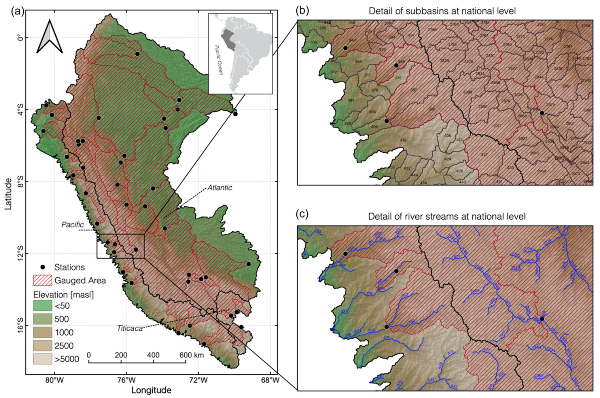
In this work, the study domain corresponds to the entire Peruvian territory, including transboundary basins with Ecuador, Colombia, and Brazil. It has an approximate total drainage area of 1,480,620 km2 (Figure 1). Moreover, 3594 river streams and sub-basins with a median area of 300 km2 (with extremes values of 40 km2 and 2500 km2) were delimited to obtain fine streamflow spatialization according to meteorological inputs resolution (~10 × ~10 km) and considering a unique river stream by sub-basin to compute flow accumulation. In Figure 1, gauged areas correspond to drainage areas covered by a hydrometric station, while ungauged areas correspond to areas without any hydrometric control downstream.
3. Data and Methods
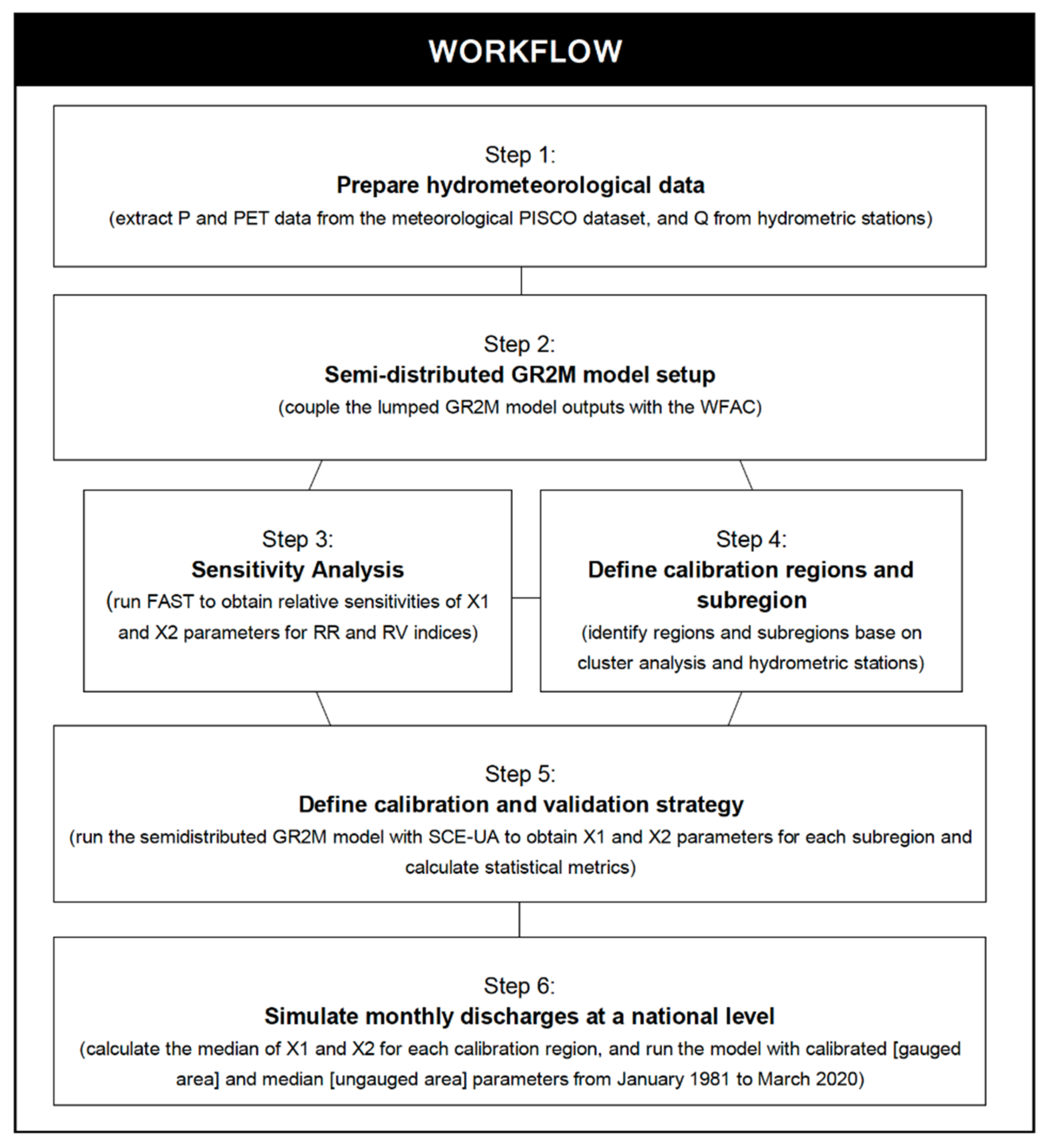
The methodology used in this study is outlined in Figure 2. The details of the data and methods used are shown below.
3.1. Hydrometeorological Data
3.1.1. The PISCO Dataset
Currently, the PISCO product is only a dataset with a daily and monthly temporal resolution for the variables of precipitation (P), air temperature (TMP), and potential evapotranspiration (PET). It has a spatial coverage throughout the Peruvian territory, including transboundary basins with Ecuador, Colombia, and Brazil. In its stable version, PISCO is only available from 1981 to 2016. However, an unstable version of the precipitation sub-product used for operative purposes is available from 1981 to the present day, and it is updating daily. The gridded precipitation sub-product (0.1° × 0.1°) is generated by applying geostatistical techniques to combine satellite estimates of precipitation data from the CHIRP project (Climate Hazards InfraRed Precipitation) and ground data of the SENAMHI pluviometric network [11]. Similarly, the temperature sub-product (0.1° × 0.1°) is generated by combining air temperature data from MODIS images and observations from weather stations. The evapotranspiration sub-product (0.1° × 0.1°) is generated from the previous temperature-gridded data following the methodology proposed by [49]. The PISCO dataset is available on the IRI Data Library: http://iridl.ldeo.columbia.edu/SOURCES/.SENAMHI/.HSR/.PISCO (accessed on 20 March 2019).
In this work, the mean areal values of P and PET are calculated for each of the 3594 sub-basins from January 1981 to March 2020 and then are continuously updating for operational purposes of the continuous monthly streamflows estimation. Due to our hydrological model’s operational purpose, the precipitation sub-products unstable version was used in this study. In contrast, in evapotranspiration, we only use climatological values due to the lack of data since January 2017.
3.1.2. Discharge Data
In this work, monthly observed streamflows at 43 hydrometric stations were selected from January 1981 to March 2020. Most of these stations belong to the National Service of Meteorology and Hydrology of Peru (SENAMHI, https://www.gob.pe/senamhi, accessed on 13 March 2021). Specifically, in the Amazon region (Atlantic slope), most of the stations are monitored by the SENAMHI and the IRD (French Institute for Sustainable Development) in the frame of the HYBAM Project (https://hybam.obs-mip.fr/, accessed on 25 March 2021). The detail of selected stations is summarized in Table 1, and their distribution throughout the Peruvian territory is shown in Figure 1a. The selection processes considered stations with more than 10% coverage in the study period (1981–2020), stations with high quality of data, and stations located in basins that guarantee coverage throughout the national territory. Finally, a total of 74.8% of the study area is gauged by the 43 hydrometric stations selected, and only 25.2% correspond to ungauged areas.
3.2. Semi-Distributed GR2M Model
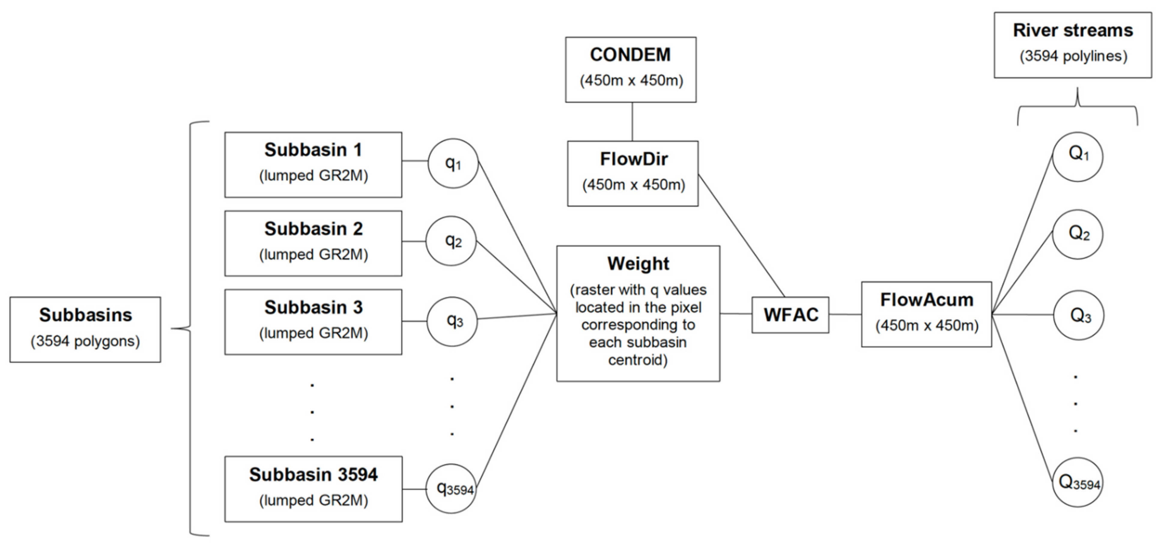
In this study, the GR2M conceptual model [50] simulates monthly runoff in 3594 sub-basins. The GR2M model transforms rainfall into runoff by two equations: production and transfer functions [51], and requires monthly input data of precipitation (P) and potential evapotranspiration (PET). P is distributed in the upper storage tank (S) with limited capacity and the underground storage reservoir (R). Besides, GR2M has two calibratable parameters (X1 and X2), where X1 defines the maximum capacity of S and X2 defines the exchange between R water outside the basin. Because GR2M is a lumped model, the simulated runoff in each sub-basin is then routed (as FlowAcum) considering the flow direction (FlowDir) generated from a 90 m HydroSHEDS Hydrologically Conditioned Digital Elevation Model (CONDEM) [52] and a Weighted Flow Accumulation (WFAC) algorithm where the simulated runoff gives the weighting factor (Weight) in each sub-basin. For example, at time step t = 1, the monthly runoff (q) is first calculated for each sub-basin in the study area. Then the Weight is created by rasterizing the sub-basins based on the flow direction raster and associating the value of q to the pixel corresponding to the centroid of each sub-basin, as appropriate. Finally, the WFAC is used to accumulate the values of q and obtain a raster map with the values of discharges (Q) for each river stream. This process is repeated for each time step. The scheme of the semi-distributed GR2M adaptation for a national level modeling is shown in Figure 3.
In this work, the GR2M model incorporated in the airGR R package [52] was used together with adaptations to calculate P and PET’s areal means from gridded data, run the semi-distributed GR2M model using the WFAC algorithm, and automatically calibrate the model parameters. As a result of this process, an experimental R package called GR2MSemiDistr was generated and is free available on https://github.com/hllauca/GR2MSemiDistr (accessed on 13 March 2021).
3.3. Sensitivity Analysis
Similar to [53], the spatial patterns and the magnitude of the relative sensitivities of X1 and X2 concerning two hydroclimatic indices are considered the basis for delimiting the homogeneous calibration regions at a national level. Unlike studies that perform a sensitivity analysis (SA) using metrics such as the Nash-Sutcliffe efficiency index [54], this study examines the sensitivity based on the runoff rate (RR) and the runoff variability (RV) hydroclimatic indices proposed by [55]. Table 2 describes both indices and their respective equations. Fourier amplitude sensitivity testing (FAST) [56] was applied using the fast R package of [55] to calculate the relative sensitivities of X1 and X2 for both indices in all sub-basins. An ensemble of 1000 unique and uncorrelated parameters was generated. The GR2M model was then run at a national level for each ensemble member using the same P and PET forcing data, yielding thousands of streamflows time series and RR and RV indices. Finally, a Fourier transformation is applied to RR and RV, and results are scaled from 0 to 1 to obtain the X1 and X2 relative sensitivities. Zero values indicate a low sensitivity of the hydroclimatic index to a GR2M parameter variation, and 1 indicates a high sensitivity. The details of the FAST methodology are found in [57].
3.4. Calibration Regions and Sub-Regions
RR and RV’s relative sensitivities calculated in the previous section and proximity variables (latitude and longitude) concerning each sub-basin’s centroid were used for cluster analysis. Then, Ward’s hierarchical clustering method based on L-moment statistics [58] was used to divide the sub-basins into homogeneous regions. Finally, the regions are hydrologically conditioned according to the discordancy and heterogeneity statistics done in [59] and including at least one hydrometric station in the calibration region. In the absence of a station within the previously defined region, neighboring regions are merged to ensure this condition.
Due to the low density of hydrometric stations in the study area providing a long record of monthly streamflows for the model calibration (Figure 1a and Table 2) and the effect of equifinality of the parameters [60], sub-regions are restricted to the portion-gauged by hydrometric stations within each calibration region. These sub-regions are defined by superimposing the calibration regions and gauged areas’ boundaries (Figure 1a). Thus, there will be as many sets of calibrated GR2M parameters for a given region as there are sub-regions within it. In the case of ungauged areas, only the calibration regions are considered.
3.5. GR2M Calibration and Validation Strategy
In this work, 43 hydrometric stations are used to calibrate and validate Peru’s water balance model. The selected calibration period for the hydrometric stations ranging from 60 to 70% of their available records. The P and PET climatologies (1981–2010) were used to fill data between January 1978 and December 1980 and consider them a warm-up period for national simulation. Parameters X1 and X2 were automatically calibrated using the Shuffled Complex Evolutionary (SCEA-UA) algorithm [61], considering the Kling–Gupta efficiency criterion (KGE) [61] as an objective function similar to [62] with an emphasis on high flows. The square root transferred Nash–Sutcliffe efficiency (NSEsqrt) [62] is used to evaluate model performance in general flows, and the Water Balance Error (WBE) [63] was used to assess the model bias. The summary of the statistical metrics used and their corresponding equations are shown in Table 3. The validation process consisted of evaluating the model’s outputs based on the previously calibrated parameters using the remaining 30–40% of the available streamflow records.
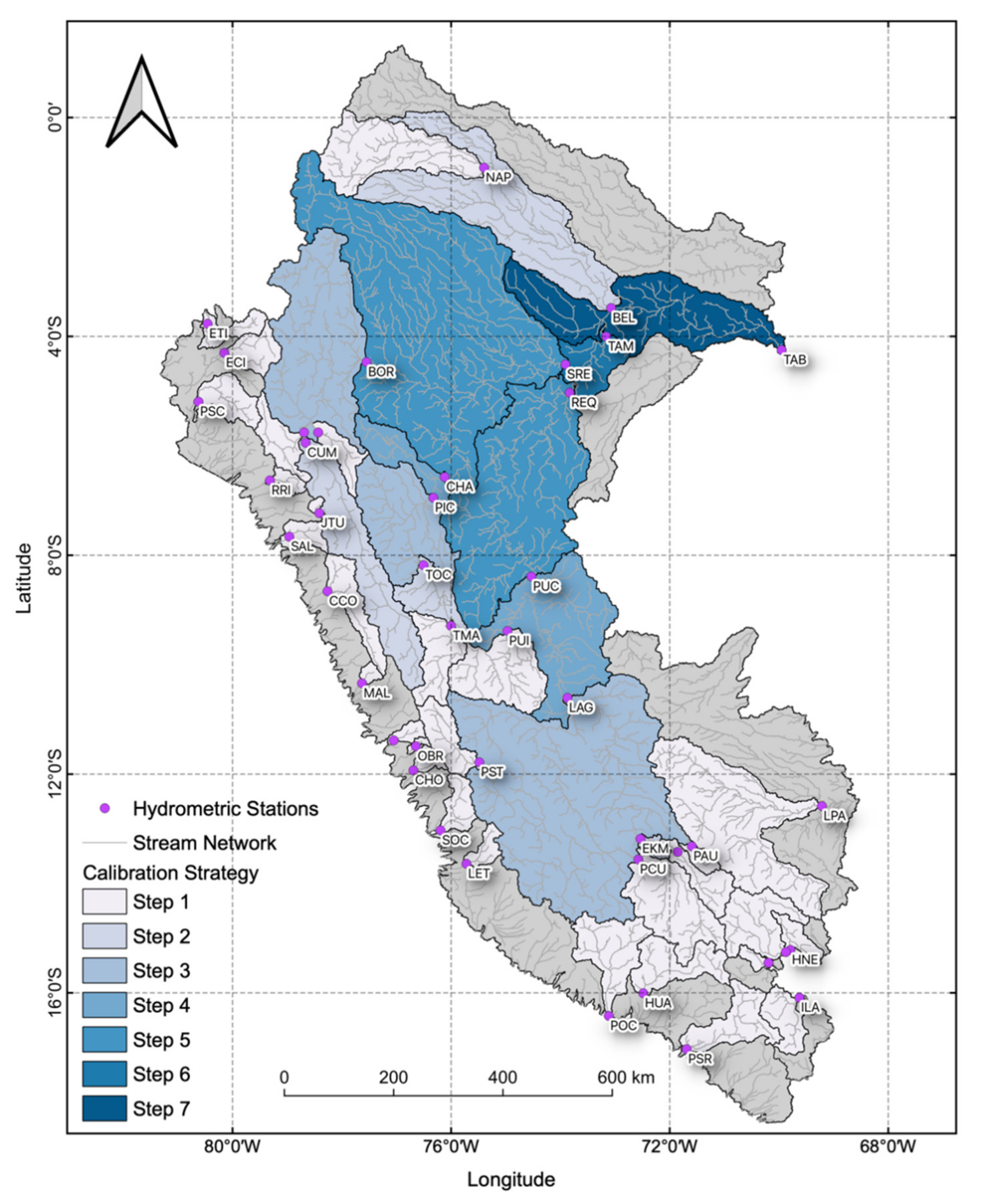
The model calibration and validation were performed in gauged areas, and a stepwise calibration strategy was used in this study (sub-region approach, Figure 4). In the first step, the parameters of headwater sub-basins are calibrated and are used downstream, while in the last step, only the parameters of the remaining sub-basins are calibrated. The sub-basins of the Pacific and the Titicaca slopes were calibrated in a unique step, while for the Atlantic slope, seven steps were required. Finally, after model calibration and validation for each sub-region, X1 and X2 values are grouped by calibration region at a national level.
3.6. Discharge Simulation at a National Level
The median of X1 and X2 is calculated for each calibration region to simulate monthly discharges in ungauged areas (regional approach). To assess the model performance when using the median of X1 and X2 as a representative parameter for each calibration region, the GR2M model was again run-in gauged areas, and new statistical metrics were calculated. Moreover, changes in model performance before and after applying the median of parameters by calibration regions were evaluated. Finally, a new model run including gauged and ungauged areas was executed to simulate monthly discharges in 3594 river streams.
4. Results
4.1. Sensitivity Analysis and Calibration Regions
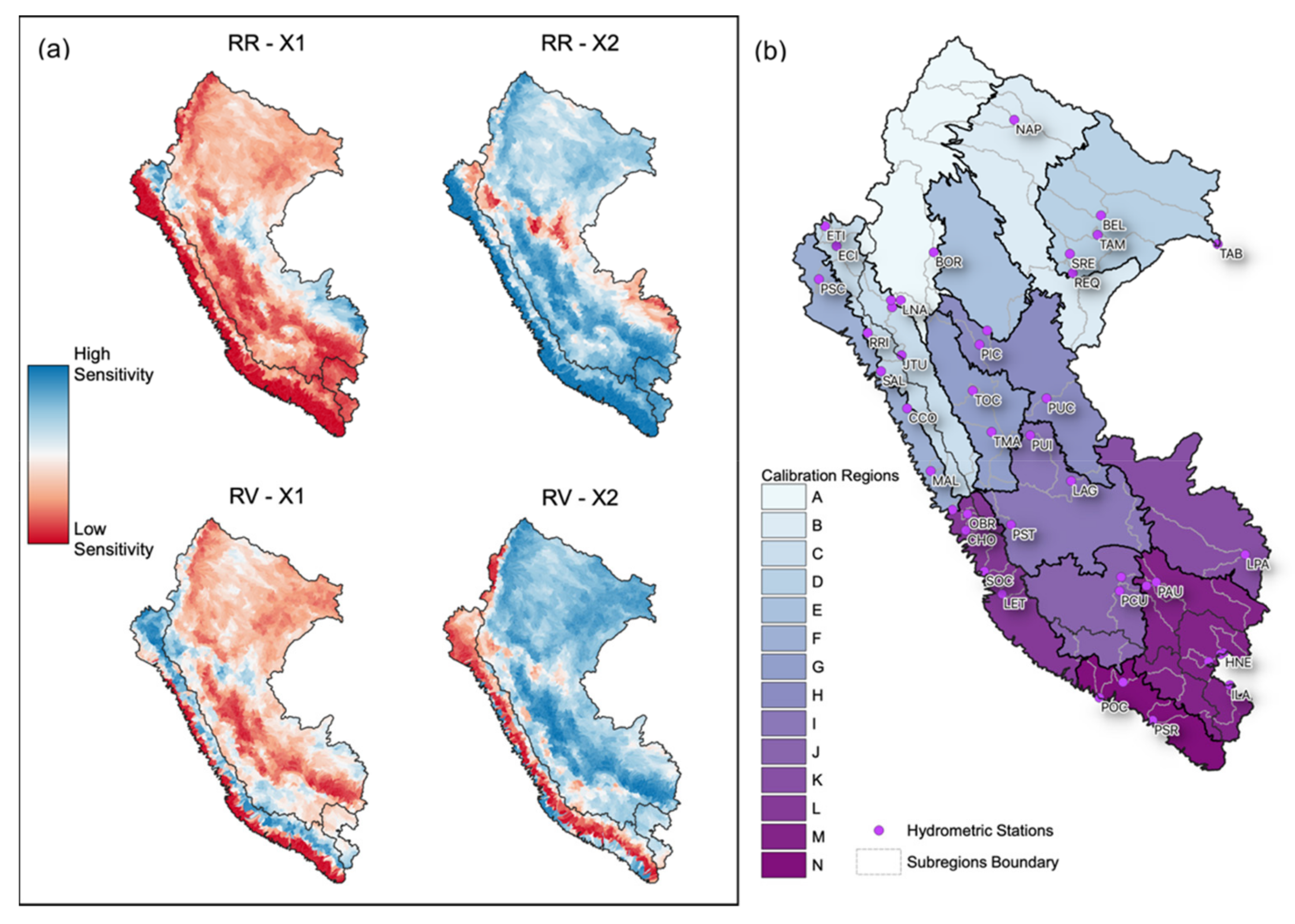
The relative sensitivities derived from the FAST analysis using the RR and RV indices for each of the 3594 sub-basins throughout the study area are shown in Figure 5a. Because the GR2M model has only two parameters, the patterns of relative sensitivities to X1 and X2 are inverse. This study assesses the hydrological response in terms of the magnitude (RR) and variability (RV) of the rainfall–runoff relationship. RR and RV indices are more sensitive to X2 over much of the study area. Especially on the Pacific slope, RR has high sensitivities to X2 in coastal sub-basins but declines slightly towards the Andes’ western flank. On the Titicaca and Atlantic slopes, moderate to high sensitivities to X2 is observed, except for the central part of the Amazon extending southeast and to part of the North Pacific, where there are high sensitivities to X1. In RV, spatial patterns are like RR but with greater sensitivities relative to X2 in the major part of the Atlantic and the Titicaca slopes, while in the Pacific slope, sensitivities to X1 increase in the west flank of the Andes and the North Pacific sub-basins.
The clustering analysis results incorporating the relative sensitivity patterns of RR and RV at a national level are shown in Figure 5b. The lack of hydrometric information in some of the initial regions meant having to merge contiguous regions, so 14 regions were identified throughout the study area. In the coast of the Pacific, three regions were identified (F, L, and N); in the Andes–Amazon transition, five regions were obtained (C, G, I, J, and M), while six regions (A, B, D, E, H, and K) were obtained in the Amazon lowlands. It was ensured that there was at least one hydrometric station for each of the calibration regions (as is the case for regions B, E, and K), while in some cases, regions with more than five stations (M and C) were obtained (Table 4).
Finally, overlapping the boundaries of gauged and ungauged sub-basins (Figure 4) with the 14 calibration regions (Figure 5b) generated 96 sub-regions (Table 4), which corresponds to 96 different sets of GR2M parameters. Of these, 84 parameter sets are estimated by model calibration (sub-region approach), while the remaining 12 were inferred based on the median values for each calibration region (regional approach).
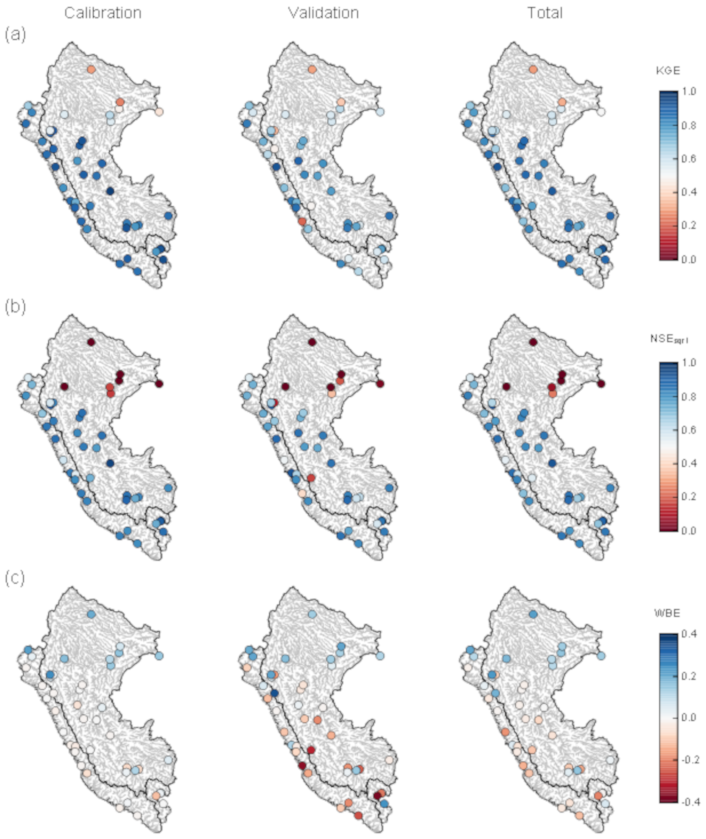
4.2. Model Performance Assessment
Figure 6 shows the spatial distribution of the three metrics selected to assess the monthly water balance model’s performance at a national level during its calibration, validation, and entire period. In terms of KGE and NSEsqrt, the model performs well during the calibration period, with values above 0.75 and 0.65, respectively, at stations on the Pacific and the Andes–Amazon transition; however, low values of KGE and NSEsqrt (<0.50) predominate at stations on the Amazon lowlands. Performance remains the same during validation but with a slight decrease in the KGE and NSEsqrt metrics at stations belonging to the Andes–Amazon transition. Regarding the WBE, balance errors close to zero during the calibration period are observed at stations with high KGE and NSEsqrt values, except for positive balance errors not greater than 0.25 at stations in the Amazon lowlands. Negative balance errors increase in the validation period, up to −0.38 on the Pacific coast and the Andes–Amazon transition.
When evaluating the total period, good model performance in terms of KGE (KGE ≥ 0.75) is maintained for 71% of the stations. In the same period, NSEsqrt values higher than 0.65 for 70% of the stations demonstrate a good representation of the sub-basin’s general flows. In terms of the WBE, negative values of not less than −0.20 are evident at most of the stations with high KGE and NSEsqrt values, and positive values of not more than 0.23 are evident for the Amazon lowlands. This behavior indicates that stations with a good fit in terms of KGE and NSEsqrt tend to slightly overestimate the total runoff, while on the Amazon lowlands, it tends to be underestimated.
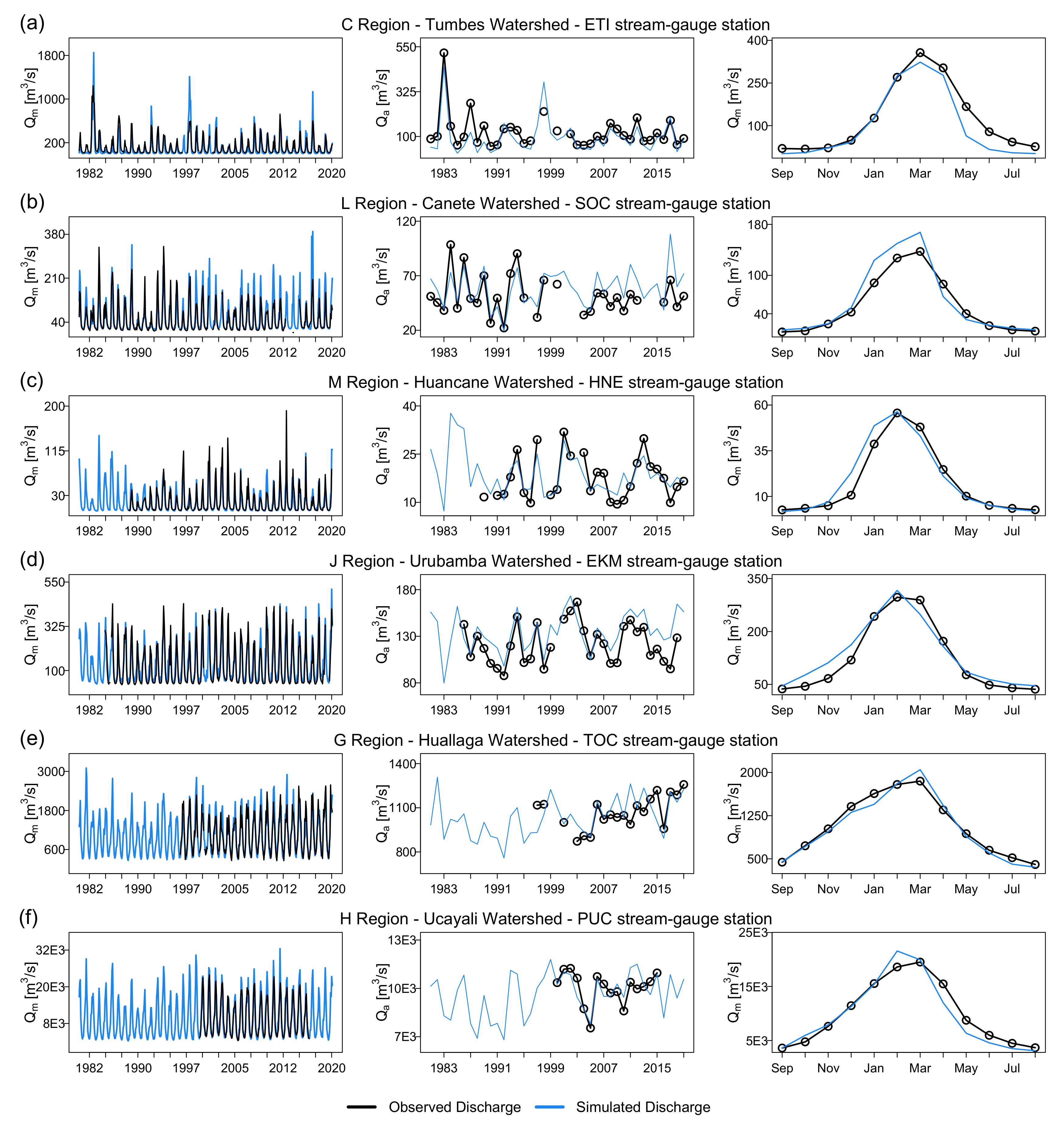
Figure 7 shows the observed and simulated monthly and annual hydrographs and their respective seasonal variation curves for two hydrometric stations on the Pacific slope (ETI and SOC), one on the Titicaca slope (HNE), and three on the Atlantic slope (EKN, TOC, and PUC), corresponding to stations with extensive streamflow records from January 1981 to March 2020 (Table 1). In all cases, the model manages to represent the seasonal and interannual variability of the observations in both small basins of 65 m3/s average annual flow (Cañete basin) up to basins with 9000 m3/s (Ucayali basin). The simulated series fit very well to the observations at most of the stations evaluated, except for SOC, where the wet season’s streamflows (December–March) were slightly overestimated. At an annual scale, the model can represent very dry (e.g., 1991 and 1992) to very wet years (e.g., 1997) in sub-basins of the three Peruvian slopes. The seasonal variation curves adequately represent the peak flow month, except for the PUC station, where there is one lag month (Figure 7d). This adequate seasonal and interannual representation is repeated in the remaining hydrometric stations (not shown), except for those located in the Amazon lowlands, where the monthly model performs poorly in terms of NSEsqrt (Figure 6b).
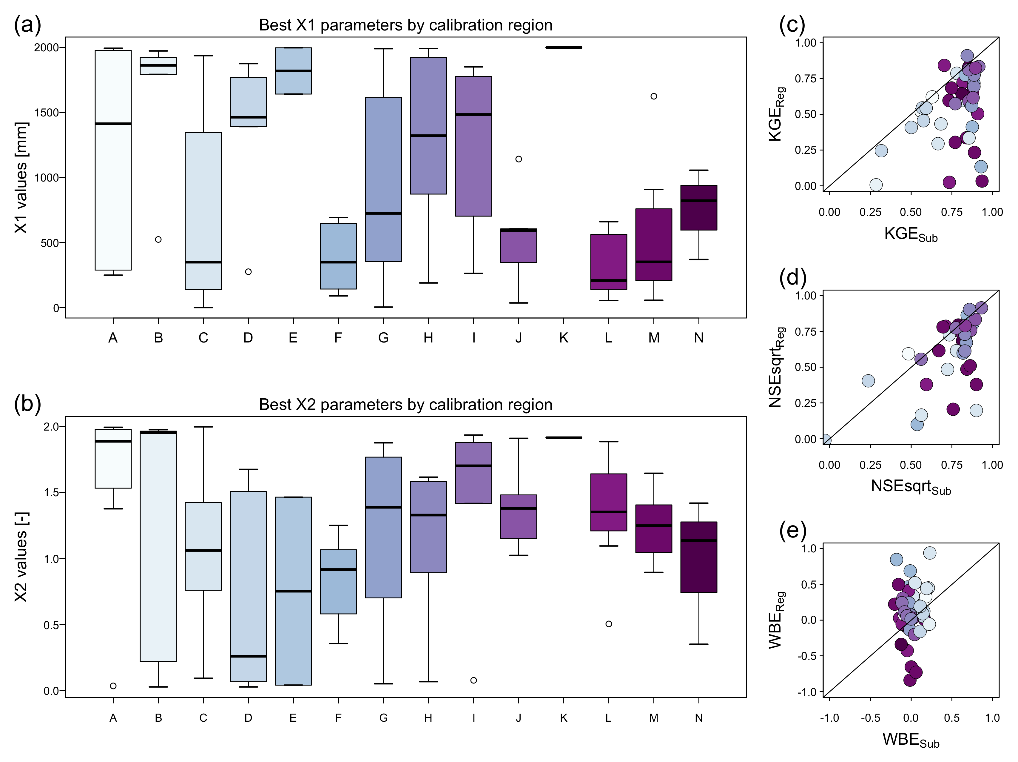
The variation of the calibrated GR2M model parameters in the gauged areas is shown in the boxplots of Figure 8a,b. In [31] reports that X1 could take values from 0.1 to 2000 mm while X2 could vary between 0 and 2. There are slight variations of X1 and X2 in calibration regions located in the south of the country (J, K, L, M, and N; see Figure 5b) and north-central coast regions (F; see Figure 5b). Also, there are slight variations of X1 and high variation of X2 in calibration regions located in the northeast of the country (B, D, and E; see Figure 5b), predominantly in the Amazon lowlands. Additionally, we identified high variations of X1 values and low variations of X2 in regions of the north-central Andes (A, C, H, and I; see Figure 5b). Only in the calibration region G, high variations in both X1 and X2 values are present (Figure 8a,b). It is important to notice that regions with high X2 variations in Figure 8a,b coincide with stations of low performances in terms of KGE and NSEsqrt (Figure 6a,b). In contrast, the regions with smaller variations in both X1 and X2 parameter values correspond to stations with a good model fit.
Figure 8c–e shows the model performance variation before (sub-region approach—Sub) and after (regional approach—Reg) applying the median of GR2M parameters by each calibration region. In terms of the KGE and NSEsqrt, the model performance using the regional approach (Figure 8c,d) declines mainly in sub-basins of the A–D regions (see Figure 5b) and is relatively stable (except for region M) in south-central regions. Since ungauged areas are located predominantly in regions F, L, and N, the regional approach of parameters in these sub-basins is suitable for estimating monthly discharges.
4.3. Product of Simulated Monthly Discharges at a National Level
The regionalization based on sensitivity analysis of GR2M parameters at a national level and using the meteorological (P and PET) PISCO dataset allows simulating continuous monthly discharges in 3594 rivers streams (including ungauged areas) from January 1981 to March 2020. This new product of simulated monthly discharges named PISCO_HyM_GR2M is available at https://doi.org/10.6084/m9.figshare.14382758 (accessed on 7 April 2021), and it is the new hydrological sub-product of the PISCO dataset. Additionally, it will contribute to the understanding of the water balance in data-scarce basins. For instance, the PISCO_HyM_GR2M product is currently used for drought monitoring in the National Service of Meteorology and Hydrology of Peru (available online: https://www.senamhi.gob.pe/?p=monitoreo-pronostico-sequias—accessed on 14 January 2021).
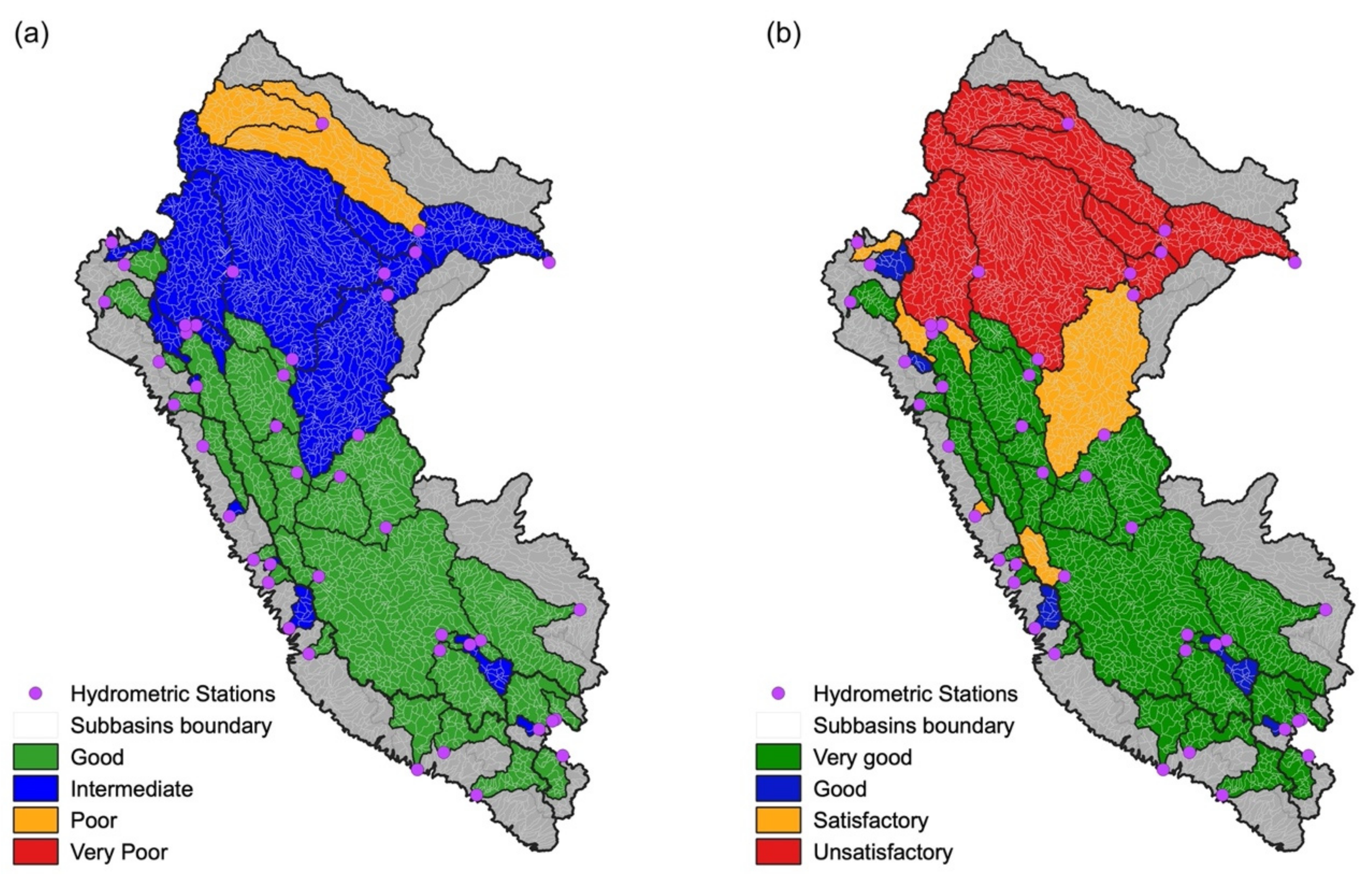
The qualitative classification of the PISCO_HyM_GR2M simulations, based on KGE [63] and NSEsqrt [64] performance categories for gauged areas are shown in Figure 9a,b, respectively. Both metrics agree that simulated monthly discharge in the central and southern of the study area are well represented, while those for the northeast (Amazon lowlands) should be interpreted with caution. The latter varies depending on the hydrograph assessment approach because the KGE metric emphasizes high flows [65], while NSEsqrt reduces this effect and emphasizes the general representation of streamflows [64].
5. Discussion
5.1. Sensitivity Analysis and Calibration Regions
In this paper, two conceptual parameters’ relative sensitivities are used as main predictors to define calibration regions at a national level similar to [21], instead of traditional climatic and physiographical characteristics [15]. Despite the differences between objective functions selected (RR and RV, Table 2), the spatial patterns of relative sensitivities for GR2M parameters are very similar in both cases (Figure 5a) due to the parsimonious model structure [31,34], finding that X2 is the most sensitive parameter for RR and RV indices in a great number of sub-basins due to its correction role in runoff generation [18] instead of X1 in charge of controlling soil moisture in the production storage. In terms of GR2M outputs, we found that a slight variation of X2 (controlling the routing storage) can significantly alter the rainfall–runoff transformation in many basins nationwide due to changes in the magnitude and variability of the simulated runoff.
The results showed main differences in RR and RV sensitivities spatial patterns in the Pacific Slope (see Figure 5a) due to X2—that controls water exchange and groundwater fluxes as mention in [65]—is more relevant for RR in coastal sub-basins where GR2M runoff is base flow-dominated [66] than in mountain ranges areas where X1 has more relative sensitivity for RV. However, in the behavior in the central-northern Amazonian region (Atlantic slope), abrupt changes in X1-X2 sensitivities might be more related to model inputs biases and structural uncertainties that propagate to model parameters and outputs.
As the regionalization approach is based on the sensitivity analysis of a parsimonious conceptual model (see Section 3.3), calibration regions delimited (Figure 5b) represent areas with a similar level of parameter uncertainties [65] and hydrological model response [65], instead of providing similarities of geomorphological and climatic such as present in [66]. Thus, calibration regions generated in this work are only valid for the GR2M water balance model using the PISCO product as meteorological inputs.
In addition to the relative sensitivities calculated in this work, the hydrometric network at the national level plays an important role in the final delimitation of the calibration regions and sub-regions (Figure 5b) because the existence of at least one of them is a determining factor. In this sense, unlike the studies by [67] where parameter uncertainty bounds are identified based on residuals analysis of hydrometric stations by region, the low density of stations (Figure 4), mainly on the north Atlantic slope, could be altering the natural grouping of sub-basins and thus reducing the predictive capacity of regional parameters of the GR2M model (see Section 4.2) based on a sensitivity analysis. Future studies will assess regional parameter uncertainty in uncontrolled areas and impact discharge estimation.
5.2. Model Simulations at a National Level
The unsatisfactory results in the northern Amazonian region (Figure 9) reflects two issues: first, the greater uncertainty of the spatial rainfall distribution in the Marañón [49], Ucayali and Huallaga [49,68] basins, and the PISCOP sub-product biases probably because of the lack of adequate rainfall estimates in equatorial regions [11]. This lower model performance is similar to that were obtained in [67,68] using different hydrological models in a daily timestep and different sets of satellite precipitation products. Thus, rainfall uncertainties propagate to model outputs and reduce the model’s predictable capacity [26]. Additionally, PET climatology used in this paper for operational purposes might not be reflecting actual evapotranspiration in the Amazon plain. Future works will incorporate a robust assessment of evapotranspiration in the hydrological modeling with a data scares scenario and its impacts on the water balance.
Secondly, floodplain plays a key role in the flow routing, with a large amount of water stored during the flood [69]. For instance, in the Ucayali basin, the flood peak is delayed by two months between the LAG and REQ stations [70,71]. These behaviors might alter basins storage and delay months of peak flow in basins with larger drain areas such as the Amazon plain, and GR2M routing might not represent this characteristic such as PUC station in Figure 7d.
It is also important to consider that GR2M is a model with limitations due to the conceptualization of hydrological processes in two reservoirs (production and routing) in a lumped modeling approach [33]. Despite its outstanding performance throughout the national territory (Figure 6), it may not be able to adequately represent runoff in basins with large drainage areas (>200,000 km2) such as in the Amazon plain. Future works will incorporate routing models such as the Routing Application for Parallel computatIon of Discharge (RAPID) [72] to improve flow routing throughout the national drainage network, especially in the Atlantic slope.
6. Conclusions
This study evaluated a monthly water balance model’s hydrological performance in 3594 sub-basins and river streams in Peru. Parameter calibration regions were defined based on the sensitivity analysis of two hydroclimatic indices. Finally, the monthly simulated streamflows product named PISCO_HyM_GR2M from January 1981 to March 2020 was developed. The main conclusions are summarized below:
- (a)
- The hydrological performance of the GR2M model in Peru performed well in sub-basins of the Pacific slope and the Andes–Amazon transition (part of the Titicaca and the Atlantic slopes). The model adequately represents the seasonality and interannual variability of the streamflows, except for the Amazon lowlands, where only high flows are well-represented.
- (b)
- Through the monthly meteorological PISCO sub-products, it is possible to simulate the runoff volume over most of Peru adequately. However, the uncertainties associated with these sub-products are more significant towards the north of the country where there are not enough meteorological stations, so this error propagates towards the hydrological model outputs for the Amazon lowlands.
- (c)
- The proposed methodology to define the calibration regions based on the spatial patterns of two hydroclimatic indices’ relative sensitivities proved to be an appropriate technique for calibrating and validating the GR2M model and estimating monthly discharge in ungauged sub-basins.
The results presented in this work also demonstrate the enormous potential of the PISCO_HyM_GR2M product for understanding the dynamics of surface water resources in Peru. Future versions of this product will include an extensive analysis of different routing methods and the uncertainty analysis of discharges.
Author Contributions
Conceptualization, H.L. and W.L.-C.; methodology, H.L., W.L.-C. and C.M.; software, H.L.; validation, H.L., C.M., W.L.-C., W.S. and P.R.; formal analysis, H.L. and W.L.-C.; investigation, H.L., W.L.-C. and C.M.; resources, W.L.-C., W.S. and P.R.; data curation, H.L. and C.M.; writing—original draft preparation, H.L.; writing—review and editing, H.L., W.L.-C., W.S. and P.R.; visualization, H.L.; supervision, W.L.-C.; project administration, W.L.-C.; funding acquisition, W.S. and P.R. All authors have read and agreed to the published version of the manuscript.
Funding
This research was funding by Institut de Recherche pour le Développement (IRD), France, through the HYBAM program.
Institutional Review Board Statement
Not applicable.
Informed Consent Statement
Informed consent was obtained from all subjects involved in the study.
Data Availability Statement
The data presented in this study are publicly available online in https://doi.org/10.6084/m9.figshare.14382758 (accessed on 7 April 2021), and on the IRI Data Library repository http://iridl.ldeo.columbia.edu/SOURCES/.SENAMHI/.HSR/.PISCO/ (accessed on 7 April 2021).
Acknowledgments
The authors extend their appreciation to the anonymous reviewers for their thoughtful comments and valuable advice. A special acknowledgment to the International Research Institute for Climate and Society (IRI) team for supporting PISCO data distribution publicly. P. Rau acknowledges supports from the Newton Paulet fund (NERC-CONCYTEC) through the RAHU project (005-2019-FONDECYT).
Conflicts of Interest
The authors declare no conflict of interest.
References
- ANA. Plan Nacional de Recursos Hídricos del Perú; Autoridad Nacional del Agua: Lima, Perú, 2013; ISBN 9786124655241.
- Biswas, A.K. Integrated water resources management: A reassessment: A water forum contribution. Water Int. 2004, 29, 248–256. [Google Scholar] [CrossRef]
- Eda, L.E.H.; Chen, W. Integrated Water Resources Management in Peru. Procedia Environ. Sci. 2010, 2, 340–348. [Google Scholar] [CrossRef] [Green Version]
- Budds, J.; Hinojosa, L. Restructuring and Rescaling Water Governance in Mining Contexts: The Co-Production of Waterscapes in Peru. Water Altern. 2012, 5, 119. [Google Scholar]
- Paturel, J.E.; Ouedraogo, M.; Mahe, G.; Servat, E.; Dezetter, A.; Ardoin, S. The influence of distributed input data on the hydrological modelling of monthly river flow regimes in West Africa. Hydrol. Sci. J. 2003, 48, 881–890. [Google Scholar] [CrossRef]
- Louvet, S.; Paturel, J.E.; Mahé, G.; Rouché, N.; Koité, M. Comparison of the spatiotemporal variability of rainfall from four different interpolation methods and impact on the result of GR2M hydrological modeling—case of Bani River in Mali, West Africa. Theor. Appl. Climatol. 2016, 123, 303–319. [Google Scholar] [CrossRef]
- Turan, M.E.; Yurdusev, M.A. Fuzzy Conceptual Hydrological Model for Water Flow Prediction. Water Resour. Manag. 2016, 30, 653–667. [Google Scholar] [CrossRef]
- Mazrooei, A.; Sankarasubramanian, A. Improving monthly streamflow forecasts through assimilation of observed streamflow for rainfall-dominated basins across the CONUS. J. Hydrol. 2019, 575, 704–715. [Google Scholar] [CrossRef]
- Adane, G.B.; Hirpa, B.A.; Gebru, B.M.; Song, C.; Lee, W.-K. Integrating Satellite Rainfall Estimates with Hydrological Water Balance Model: Rainfall-Runoff Modeling in Awash River Basin, Ethiopia. Water 2021, 13, 800. [Google Scholar] [CrossRef]
- Llauca, H.; Lavado-Casimiro, W.; León, K.; Jimenez, J.; Traverso, K.; Rau, P. Assessing Near Real-Time Satellite Precipitation Products for Flood Simulations at Sub-Daily Scales in a Sparsely Gauged Watershed in Peruvian Andes. Remote Sens. 2021, 13, 826. [Google Scholar] [CrossRef]
- Aybar, C.; Fernández, C.; Huerta, A.; Lavado, W.; Vega, F.; Felipe-Obando, O. Construction of a high-resolution gridded rainfall dataset for Peru from 1981 to the present day. Hydrol. Sci. J. 2020, 65, 770–785. [Google Scholar] [CrossRef]
- Kratzert, F.; Klotz, D.; Shalev, G.; Klambauer, G.; Hochreiter, S.; Nearing, G. Towards Learning Universal, Regional, and Local Hydrological Behaviors via Machine-Learning Applied to Large-Sample Datasets. Hydrol. Earth Syst. Sci. 2019, 23, 5089–5110. [Google Scholar] [CrossRef] [Green Version]
- Abou Rafee, S.A.; Uvo, C.B.; Martins, J.A.; Domingues, L.M.; Rudke, A.P.; Fujita, T.; Freitas, E.D. Large-Scale Hydrological Modelling of the Upper Paraná River Basin. Water 2019, 11, 882. [Google Scholar] [CrossRef] [Green Version]
- Lane, R.A.; Coxon, G.; Freer, J.E.; Wagener, T.; Johnes, P.J.; Bloomfield, J.P.; Greene, S.; Macleod, C.J.A.; Reaney, S.M. Benchmarking the predictive capability of hydrological models for river flow and flood peak predictions across over 1000 catchments in Great Britain. Hydrol. Earth Syst. Sci. 2019, 23, 4011–4032. [Google Scholar] [CrossRef] [Green Version]
- Pagliero, L.; Bouraoui, F.; Diels, J.; Willems, P.; McIntyre, N. Investigating regionalization techniques for large-scale hydrological modelling. J. Hydrol. 2019, 570, 220–235. [Google Scholar] [CrossRef]
- Drogue, G.; Ben Khediri, W. Catchment model regionalization approach based on spatial proximity: Does a neighbor catchment-based rainfall input strengthen the method? J. Hydrol. Reg. Stud. 2016, 8, 26–42. [Google Scholar] [CrossRef] [Green Version]
- Wagener, T.; Sivapalan, M.; Troch, P.; Woods, R. Catchment Classification and Hydrologic Similarity. Geogr. Compass 2007, 1, 901–931. [Google Scholar] [CrossRef]
- Rau, P.; Bourrel, L.; Labat, D.; Ruelland, D.; Frappart, F.; Lavado, W.; Dewitte, B.; Felipe, O. Assessing multidecadal runoff (1970–2010) using regional hydrological modelling under data and water scarcity conditions in Peruvian Pacific catchments. Hydrol. Process. 2019, 33, 20–35. [Google Scholar] [CrossRef] [Green Version]
- Beck, H.E.; van Dijk, A.I.J.M.; de Roo, A.; Miralles, D.G.; McVicar, T.R.; Schellekens, J.; Bruijnzeel, L.A. Global-scale regionalization of hydrologic model parameters. Water Resour. Res. 2016, 52, 3599–3622. [Google Scholar] [CrossRef] [Green Version]
- Narbondo, S.; Gorgoglione, A.; Crisci, M.; Chreties, C. Enhancing Physical Similarity Approach to Predict Runoff in Ungauged Watersheds in Sub-Tropical Regions. Water 2020, 12, 528. [Google Scholar] [CrossRef] [Green Version]
- Bock, A.R.; Hay, L.E.; McCabe, G.J.; Markstrom, S.L.; Atkinson, R.D. Parameter regionalization of a monthly water balance model for the conterminous United States. Hydrol. Earth Syst. Sci. 2016, 20, 2861–2876. [Google Scholar] [CrossRef] [Green Version]
- Pagliero, L.; Bouraoui, F.; Willems, P.; Diels, J. Large-scale hydrological simulations using the soil water assessment tool, protocol development, and application in the danube basin. J. Environ. Qual. 2014, 43, 145–154. [Google Scholar] [CrossRef] [PubMed]
- Zamoum, S.; Souag-Gamane, D. Monthly streamflow estimation in ungauged catchments of northern Algeria using regionalization of conceptual model parameters. Arab. J. Geosci. 2019, 12, 342. [Google Scholar] [CrossRef]
- Abdollahi, K.; Bashir, I.; Verbeiren, B.; Harouna, M.R.; Van Griensven, A.; Huysmans, M.; Batelaan, O. A distributed monthly water balance model: Formulation and application on Black Volta Basin. Environ. Earth Sci. 2017, 76, 198. [Google Scholar] [CrossRef]
- Xie, Z.; Yuan, F.; Duan, Q.; Zheng, J.; Liang, M.; Chen, F. Regional Parameter Estimation of the VIC Land Surface Model: Methodology and Application to River Basins in China. J. Hydrometeorol. 2007, 8, 447–468. [Google Scholar] [CrossRef] [Green Version]
- Liu, Y.; Gupta, H.V. Uncertainty in hydrologic modeling: Toward an integrated data assimilation framework. Water Resour. Res. 2007, 43, 160. [Google Scholar] [CrossRef]
- Beven, K. Prophecy, reality and uncertainty in distributed hydrological modelling. Adv. Water Resour. 1993, 16, 41–51. [Google Scholar] [CrossRef]
- Beven, K. Changing ideas in hydrology—The case of physically-based models. J. Hydrol. 1989, 105, 157–172. [Google Scholar] [CrossRef]
- Perrin, C.; Michel, C.; Andréassian, V. Does a large number of parameters enhance model performance? Comparative assessment of common catchment model structures on 429 catchments. J. Hydrol. 2001, 242, 275–301. [Google Scholar] [CrossRef]
- Perrin, C.; Michel, C.; Andréassian, V. Improvement of a parsimonious model for streamflow simulation. J. Hydrol. 2003, 279, 275–289. [Google Scholar] [CrossRef]
- Mouelhi, S.; Michel, C.; Perrin, C.; Andréassian, V. Stepwise development of a two-parameter monthly water balance model. J. Hydrol. 2006, 318, 200–214. [Google Scholar] [CrossRef]
- Pumo, D.; Viola, F.; Noto, L.V. Generation of Natural Runoff Monthly Series at Ungauged Sites Using a Regional Regressive Model. Water 2016, 8, 209. [Google Scholar] [CrossRef] [Green Version]
- Pérez-Sánchez, J.; Senent-Aparicio, J.; Segura-Méndez, F.; Pulido-Velazquez, D.; Srinivasan, R. Evaluating Hydrological Models for Deriving Water Resources in Peninsular Spain. Sustain. Sci. Pract. Policy 2019, 11, 2872. [Google Scholar] [CrossRef] [Green Version]
- Bai, P.; Liu, X.; Liang, K.; Liu, C. Comparison of performance of twelve monthly water balance models in different climatic catchments of China. J. Hydrol. 2015, 529, 1030–1040. [Google Scholar] [CrossRef]
- Okkan, U.; Fistikoglu, O. Evaluating climate change effects on runoff by statistical downscaling and hydrological model GR2M. Theor. Appl. Climatol. 2014, 117, 343–361. [Google Scholar] [CrossRef]
- Ouhamdouch, S.; Bahir, M.; Ouazar, D.; Goumih, A.; Zouari, K. Assessment the climate change impact on the future evapotranspiration and flows from a semi-arid environment. Arab. J. Geosci. 2020, 13, 82. [Google Scholar] [CrossRef]
- Topalović, Ž.; Todorović, A.; Plavšić, J. Evaluating the transferability of monthly water balance models under changing climate conditions. Hydrol. Sci. J. 2020, 65, 928–950. [Google Scholar] [CrossRef]
- Rwasoka, D.T.; Madamombe, C.E.; Gumindoga, W.; Kabobah, A.T. Calibration, validation, parameter indentifiability and uncertainty analysis of a 2—Parameter parsimonious monthly rainfall-runoff model in two catchments in Zimbabwe. Phys. Chem. Earth Parts A/B/C 2014, 67–69, 36–46. [Google Scholar] [CrossRef]
- Huard, D.; Mailhot, A. Calibration of hydrological model GR2M using Bayesian uncertainty analysis. Water Resour. Res. 2008, 44, 206. [Google Scholar] [CrossRef] [Green Version]
- Lavado Casimiro, W.S.; Labat, D.; Guyot, J.L.; Ardoin-Bardin, S. Assessment of climate change impacts on the hydrology of the Peruvian Amazon—Andes basin. Hydrol. Process. 2011, 25, 3721–3734. [Google Scholar] [CrossRef]
- O’Connor, P.; Murphy, C.; Matthews, T.; Wilby, R.L. Reconstructed monthly river flows for Irish catchments 1766–2016. Geosci. Data J. 2020. [Google Scholar] [CrossRef]
- Duan, Q.; Schaake, J.; Andréassian, V.; Franks, S.; Goteti, G.; Gupta, H.V.; Gusev, Y.M.; Habets, F.; Hall, A.; Hay, L.; et al. Model Parameter Estimation Experiment (MOPEX): An overview of science strategy and major results from the second and third workshops. J. Hydrol. 2006, 320, 3–17. [Google Scholar] [CrossRef] [Green Version]
- Addor, N.; Newman, A.J.; Mizukami, N.; Clark, M.P. The CAMELS data set:Catchment attributes and meteorology for large-sample studies. Hydrol. Earth Syst. Sci. 2017, 21, 21. [Google Scholar] [CrossRef] [Green Version]
- Jehn, F.U.; Bestian, K.; Breuer, L.; Kraft, P.; Houska, T. Clustering CAMELS using hydrological signatures with high spatial predictability. Hydrol. Earth Syst. Sci. Discuss. 2019, 1–21. [Google Scholar] [CrossRef]
- Ren, K.; Fang, W.; Qu, J.; Zhang, X.; Shi, X. Comparison of eight filter-based feature selection methods for monthly streamflow forecasting—Three case studies on CAMELS data sets. J. Hydrol. 2020, 586, 124897. [Google Scholar] [CrossRef]
- Coxon, G.; Addor, N.; Bloomfield, J.P.; Freer, J.; Fry, M.; Hannaford, J.; Howden, N.J.K.; Lane, R.; Lewis, M.; Robinson, E.L.; et al. CAMELS-GB: Hydrometeorological time series and landscape attributes for 671 catchments in Great Britain. Earth Syst. Sci. Data 2020, 12, 2459–2483. [Google Scholar] [CrossRef]
- Chagas, V.B.P.; Chaffe, P.L.B.; Addor, N.; Fan, F.M.; Fleischmann, A.S.; Paiva, R.C.D.; Siqueira, V.A. CAMELS-BR: Hydrometeorological time series and landscape attributes for 897 catchments in Brazil. Earth Syst. Sci. Data 2020, 12, 2075–2096. [Google Scholar] [CrossRef]
- Alvarez-Garreton, C.; Mendoza, P.A.; Boisier, J.P.; Addor, N.; Galleguillos, M.; Zambrano-Bigiarini, M.; Lara, A.; Cortes, G.; Garreaud, R.; McPhee, J.; et al. The CAMELS-CL dataset: Catchment attributes and meteorology for large sample studies-Chile dataset. Hydrol. Earth Syst. Sci. 2018, 22, 5817–5846. [Google Scholar] [CrossRef] [Green Version]
- Zubieta, R.; Getirana, A.; Espinoza, J.C.; Lavado-Casimiro, W.; Aragon, L. Hydrological modeling of the Peruvian—Ecuadorian Amazon Basin using GPM-IMERG satellite-based precipitation dataset. Hydrol. Earth Syst. Sci. 2017, 21, 3543–3555. [Google Scholar] [CrossRef] [Green Version]
- Hargreaves, G.H.; Samani, Z.A. Reference crop evapotranspiration from ambient air temperature. In Proceedings of the American Society of Agricultural Engineers Meeting, Chicago, IL, USA, 17 December 1985; pp. 85–2517. [Google Scholar]
- Lehner, B.; Verdin, K.; Jarvis, A. HydroSHEDS Technical Documentation, Version 1.0; World Wildlife Fund US: Washington, DC, USA, 2006; pp. 1–27. [Google Scholar]
- Coron, L.; Thirel, G.; Delaigue, O.; Perrin, C.; Andréassian, V. The suite of lumped GR hydrological models in an R package. Environ. Model. Softw. 2017, 94, 166–171. [Google Scholar] [CrossRef]
- Nash, J.E.; Sutcliffe, J.V. River flow forecasting through conceptual models part I—A discussion of principles. J. Hydrol. 1970, 10, 282–290. [Google Scholar] [CrossRef]
- Sankarasubramanian, A.; Vogel, R.M. Hydroclimatology of the continental United States: U.S. HYDROCLIMATOLOGY. Geophys. Res. Lett. 2003, 30, 140. [Google Scholar] [CrossRef]
- Reusser, D.E.; Buytaert, W.; Zehe, E. Temporal dynamics of model parameter sensitivity for computationally expensive models with the Fourier amplitude sensitivity test. Water Resour. Res. 2011, 47, 703. [Google Scholar] [CrossRef] [Green Version]
- Reusser, D. Implementation of the Fourier Amplitude Sensitivity Test (FAST); R Package 0.51. 2008. Available online: http://www2.uaem.mx/r-mirror/web/packages/fast/fast.pdf (accessed on 5 February 2021).
- Hosking, J.R.M.; Wallis, J.R. Regional Frequency Analysis: An Approach Based on L-Moments; Cambridge University Press: Cambridge, UK, 2005; ISBN 9780521019408. [Google Scholar]
- Hassan, B.G.H.; Ping, F. Regional rainfall frequency analysis for the luanhe basin—By using L-moments and cluster techniques. APCBEE Procedia 2012, 1, 126–135. [Google Scholar] [CrossRef] [Green Version]
- Beven, K.; Binley, A. The future of distributed models: Model calibration and uncertainty prediction. Hydrol. Process. 1992, 6, 279–298. [Google Scholar] [CrossRef]
- Duan, Q.Y.; Gupta, V.K.; Sorooshian, S. Effective and Efficient Global Minimization. J. Optim. Theory Appl. 1993, 76. [Google Scholar] [CrossRef]
- Gupta, H.V.; Kling, H.; Yilmaz, K.K.; Martinez, G.F. Decomposition of the mean squared error and NSE performance criteria: Implications for improving hydrological modelling. J. Hydrol. 2009, 377, 80–91. [Google Scholar] [CrossRef] [Green Version]
- Chiew, F.H.S.; Stewardson, M.J.; McMahon, T.A. Comparison of six rainfall-runoff modelling approaches. J. Hydrol. 1993, 147, 1–36. [Google Scholar] [CrossRef]
- Thiemig, V.; Rojas, R.; Zambrano-Bigiarini, M.; De Roo, A. Hydrological evaluation of satellite-based rainfall estimates over the Volta and Baro-Akobo Basin. J. Hydrol. 2013, 499, 324–338. [Google Scholar] [CrossRef]
- Mizukami, N.; Rakovec, O.; Newman, A.J.; Clark, M.P.; Wood, A.W.; Gupta, H.V.; Kumar, R. On the choice of calibration metrics for “high-flow” estimation using hydrologic models. Hydrol. Earth Syst. Sci. 2019, 23, 2601–2614. [Google Scholar] [CrossRef] [Green Version]
- Seiller, G.; Hajji, I.; Anctil, F. Improving the temporal transposability of lumped hydrological models on twenty diversified U.S. watersheds. J. Hydrol. Reg. Stud. 2015, 3, 379–399. [Google Scholar] [CrossRef] [Green Version]
- Bock, A.R.; Farmer, W.H.; Hay, L.E. Quantifying uncertainty in simulated streamflow and runoff from a continental-scale monthly water balance model. Adv. Water Resour. 2018, 122, 166–175. [Google Scholar] [CrossRef]
- Strauch, M.; Kumar, R.; Eisner, S.; Mulligan, M.; Reinhardt, J.; Santini, W.; Vetter, T.; Friesen, J. Adjustment of global precipitation data for enhanced hydrologic modeling of tropical Andean watersheds. Clim. Chang. 2017, 141, 547–560. [Google Scholar] [CrossRef] [Green Version]
- Zubieta, R.; Getirana, A.; Espinoza, J.C.; Lavado, W. Impacts of satellite-based precipitation datasets on rainfall–runoff modeling of the Western Amazon basin of Peru and Ecuador. J. Hydrol. 2015, 528, 599–612. [Google Scholar] [CrossRef]
- Wongchuig Correa, S.; de Paiva, R.C.D.; Espinoza, J.C.; Collischonn, W. Multi-decadal Hydrological Retrospective: Case study of Amazon floods and droughts. J. Hydrol. 2017, 549, 667–684. [Google Scholar] [CrossRef] [Green Version]
- Santini, W.; Martinez, J.-M.; Guyot, J.-L.; Espinoza, R.; Vauchel, P.; Lavado, W. Estimation of erosion and sedimentation yield in the Ucayali river basin, a Peruvian tributary of the Amazon River, using ground and satellite methods. In Proceedings of the EGU General Assembly Conference Abstracts, Vienna, Austria, 27 April–2 May 2014; p. 916. [Google Scholar]
- Santini, W.; Martinez, J.-M.; Espinoza-Villar, R.; Cochonneau, G.; Vauchel, P.; Moquet, J.-S.; Baby, P.; Espinoza, J.-C.; Lavado, W.; Carranza, J.; et al. Sediment budget in the Ucayali River basin, an Andean tributary of the Amazon River. Proc. Int. Assoc. Hydrol. Sci. 2015, 367, 320–325. [Google Scholar] [CrossRef] [Green Version]
- David, C.H.; Maidment, D.R.; Niu, G.-Y.; Yang, Z.-L.; Habets, F.; Eijkhout, V. River Network Routing on the NHDPlus Dataset. J. Hydrometeorol. 2011, 12, 913–934. [Google Scholar] [CrossRef] [Green Version]
Figure 1.
(a) Study area and hydrometric stations in the Pacific, Titicaca, and Atlantic slopes. Detail of (b) sub-basins and (c) river streams used for the semi-distributed hydrological model at a national level.
Figure 1.
(a) Study area and hydrometric stations in the Pacific, Titicaca, and Atlantic slopes. Detail of (b) sub-basins and (c) river streams used for the semi-distributed hydrological model at a national level.

Figure 2.
Methodological framework. Where: P = precipitation, PET = Potential Evapotranspiration, Q = Discharge, WFAC = Weighted Flow Accumulation, FAST = Fourier Amplitude Test, RR = Rainfall-Runoff Index, RV = Runoff Variability Index, and SCE-UA = Shuffle Complex Evolutionary Algorithm.
Figure 2.
Methodological framework. Where: P = precipitation, PET = Potential Evapotranspiration, Q = Discharge, WFAC = Weighted Flow Accumulation, FAST = Fourier Amplitude Test, RR = Rainfall-Runoff Index, RV = Runoff Variability Index, and SCE-UA = Shuffle Complex Evolutionary Algorithm.

Figure 3.
Framework to calculate accumulated discharges from sub-basins to river streams in a semi-distributed GR2M adaptation. Where: q = runoff in mm, CONDEM = Hydrologically Conditioned Digital Elevation model, FlowDir = Flow Direction, WFAC = Weighted Flow Accumulation, FlowAcum = Flow Accumulation, and Q = discharges in m3/s.

Figure 4.
Strategy for the GR2M model calibration at a national level. Steps are based on the stream network configuration and location of the hydrometric stations in gauged areas. Each basin might contain more than one set of X1 and X2 parameters. Gray areas correspond to ungauged areas.
Figure 4.
Strategy for the GR2M model calibration at a national level. Steps are based on the stream network configuration and location of the hydrometric stations in gauged areas. Each basin might contain more than one set of X1 and X2 parameters. Gray areas correspond to ungauged areas.

Figure 5.
(a) Relative sensitivities of RR and RV indices obtained from FAST. (b) Delimited calibration regions and sub-regions for the GR2M model at a national level, each region contains at least one hydrometric station.
Figure 5.
(a) Relative sensitivities of RR and RV indices obtained from FAST. (b) Delimited calibration regions and sub-regions for the GR2M model at a national level, each region contains at least one hydrometric station.

Figure 6.
(a–c) Statistical metrics for evaluating the GR2M model performance at a national level during the calibration, the validation, and the total period. In terms of the KGE and NSEsqrt metrics, cold colors represent good model performance while warm colors represent inadequate model performance. In WBE, blue colors are associated with the underestimation of the total volume of surface runoff and red colors indicate the overestimation.

Figure 7.
Observed and simulated monthly and annual discharges (Qm), and seasonal variation curves, for six representatives’ hydrometric stations in the (a,b) Pacific, (c) the Titicaca, and (d–f) the Atlantic slopes, with more extended data availability from January 1981 to March 2020.
Figure 7.
Observed and simulated monthly and annual discharges (Qm), and seasonal variation curves, for six representatives’ hydrometric stations in the (a,b) Pacific, (c) the Titicaca, and (d–f) the Atlantic slopes, with more extended data availability from January 1981 to March 2020.

Figure 8.
Boxplot of calibrated (a) X1 and (b) X2 parameters for each calibration region. (c–e) Scatterplot of statistical metrics used for evaluating model performance changes using calibrated GR2M model parameters by sub-regions (Sub) and applying the median of X1 and X2 for each calibration region (Reg).

Figure 9.
Qualitative ratings of streamflow simulation result at 43 hydrometric stations across the study area, based on (a) KGE and (b) NSEsqrt values.
Figure 9.
Qualitative ratings of streamflow simulation result at 43 hydrometric stations across the study area, based on (a) KGE and (b) NSEsqrt values.


Table 1.
Hydrometric stations selected for hydrological modeling at a national level. Coverage [%] is considering from January 1981 to March 2020.
Table 1.
Hydrometric stations selected for hydrological modeling at a national level. Coverage [%] is considering from January 1981 to March 2020.
| Slope | Station | Abrev. | Latitude [°S] | Longitude [°W] | Watershed | Source | Coverage [%] |
|---|---|---|---|---|---|---|---|
| Pacific | Huatiapa | HUA | −16.008 | −72.484 | Camaná | SENAMHI | 45.3 |
| Socsi | SOC | −13.029 | −76.195 | Cañete | SENAMHI | 92.9 | |
| Santo Domingo | SDO | −11.384 | −77.050 | Chancay-Huaral | SENAMHI | 66.0 | |
| Racarumi | RRI | −6.633 | −79.317 | Lambayeque | SENAMHI | 99.8 | |
| Salinar | SAL | −7.661 | −78.961 | Chicama | SENAMHI | 92.1 | |
| Obrajillo | OBR | −11.452 | −76.622 | Chillón | SENAMHI | 58.8 | |
| El Ciruelo | ECI | −4.300 | −80.150 | Chira | SENAMHI | 97.6 | |
| Malvados | MAL | −10.340 | −77.630 | Fortaleza | JU FORTALEZA | 31.2 | |
| Pte. Ocoña | POC | −16.422 | −73.115 | Ocoña | SENAMHI | 33.3 | |
| Letrayoc | LET | −13.640 | −75.720 | Pisco | SENAMHI | 89.5 | |
| Pte. Sánchez Cerro | PSC | −5.194 | −80.623 | Piura | PE CHIRA PIURA | 49.1 | |
| Condorcerro | CCO | −8.658 | −78.262 | Santa | PE CHAVIMOCHIC | 98.1 | |
| Pte. Santa Rosa | PSR | −17.030 | −71.690 | Tambo | JU TAMBO | 92.9 | |
| El Tigre | ETI | −3.769 | −80.457 | Tumbes | SENAMHI | 97.4 | |
| Chosica | CHO | −11.930 | −76.690 | Rímac | SENAMHI | 54.7 | |
| Titicaca | Pte. Huancané | HNE | −15.216 | −69.793 | Huancané | SENAMHI | 79.7 |
| Pte. Ramis | RAM | −15.255 | −69.874 | Ramis | SENAMHI | 72.4 | |
| Pte. Unocolla | COA | −15.451 | −70.192 | Coata | SENAMHI | 74.6 | |
| Pte. Ilave | ILA | −16.088 | −69.626 | Ilave | SENAMHI | 72.6 | |
| Atlantic | Egemsa Km105 | EKM | −13.183 | −72.533 | Urubamba | SENAMHI | 86.1 |
| Borja | BOR | −4.470 | −77.548 | Marañón | HYBAM | 86.5 | |
| Jesús Tunel | JTU | −7.221 | −78.404 | Crisnejas | SENAMHI | 97.9 | |
| Cumba | CUM | −5.944 | −78.661 | Marañón | SENAMHI | 13.7 | |
| Los Naranjos | LNA | −5.756 | −78.432 | Marañón | SENAMHI | 17.5 | |
| Puente Tocache | TOC | −8.181 | −76.506 | Huallaga | SENAMHI | 58.3 | |
| Tingo María | TMA | −9.290 | −76.003 | Huallaga | SENAMHI | 51.9 | |
| Picota | PIC | −6.949 | −76.325 | Huallaga | SENAMHI | 42.3 | |
| Chazuta | CHA | −6.570 | −76.119 | Huallaga | HYBAM | 41.7 | |
| Paucartambo | PAU | −13.321 | −71.594 | Urubamba | SENAMHI | 28.8 | |
| Pisac | PIS | −13.422 | −71.855 | Vilcanota | SENAMHI | 66.5 | |
| Pte. Cunyac | PCU | −13.560 | −72.574 | Apurímac | SENAMHI | 26.5 | |
| Pte. Stuart | PST | −11.802 | −75.490 | Mantaro | ELECTROPERU | 68.8 | |
| Puerto Inca | PUI | −9.384 | −74.968 | Pachitea | HYBAM | 43.8 | |
| Tamshiyacu | TAM | −4.003 | −73.162 | Amazonas | HYBAM | 90.6 | |
| Requena | REQ | −5.030 | −73.830 | Ucayali | HYBAM | 58.5 | |
| Lagarto | LAG | −10.607 | −73.871 | Ucayali | HYBAM | 23.1 | |
| Bellavista | BEL | −3.482 | −73.073 | Napo | HYBAM | 71.2 | |
| Pte. Corral Quemado | PCQ | −5.755 | −78.692 | Marañón | SENAMHI | 13.7 | |
| La Pastora | LPA | −12.584 | −69.214 | Madre de Dios | HYBAM | 24.4 | |
| Napo | NAP | −0.917 | −75.396 | Napo | HYBAM | 40.6 | |
| Tabatinga | TAB | −4.250 | −69.950 | Amazonas | HYBAM | 87.6 | |
| Pucallpa | PUC | −8.390 | −74.530 | Ucayali | HYBAM | 43.6 | |
| San Regis | SRE | −4.513 | −73.907 | Marañón | HYBAM | 53.0 |
Table 2.
Hydroclimatic indices used for the sensitivity analysis (SA).
| Index | Unit | Equation | Description |
|---|---|---|---|
| Runoff Ratio (RR) | - | The ratio of simulated runoff to precipitation | |
| Runoff Variability (RV) | - | The standard deviation of simulated runoff to the standard deviation of precipitation |
Note: X, simulated runoff in mm; P, rainfall in mm; σX,P, standard deviation of simulated runoff and rainfall.
Table 3.
Statistical metrics and their corresponding equations used for evaluating the hydrological performance of GR2M model.
Table 3.
Statistical metrics and their corresponding equations used for evaluating the hydrological performance of GR2M model.
| Statistical Metric | Unit | Equation | Optimal Value |
|---|---|---|---|
| Kling–Gupta efficiency (KGE) | - | 1 | |
| Nash–Sutcliffe Squared (NSEsqrt) | - | 1 | |
| Water Balance Error (WBE) | - | 0 |
Note: n, number of samples; Oi, observed streamflow; Xi, simulated streamflow.
Table 4.
Resume of calibration regions delimited for the study area, including gauged and ungauged areas.
Table 4.
Resume of calibration regions delimited for the study area, including gauged and ungauged areas.
| Calibration Region | Number of Sub-Regions | Number of Sub-Basins | Number of Hydrometric Stations |
|---|---|---|---|
| A | 8 | 380 | 2 |
| B | 6 | 346 | 1 |
| C | 13 | 239 | 6 |
| D | 6 | 385 | 5 |
| E | 2 | 229 | 1 |
| F | 6 | 158 | 5 |
| G | 10 | 190 | 2 |
| H | 7 | 269 | 2 |
| I | 6 | 316 | 3 |
| J | 6 | 220 | 2 |
| K | 2 | 258 | 1 |
| L | 8 | 159 | 4 |
| M | 12 | 324 | 7 |
| N | 4 | 121 | 2 |
| Total | 96 (100.0%) | 3594 (100.0%) | 43 (100.0%) |
| Gauged area | 84 (87.5%) | 2605 (72.5%) | 43 (100.0%) |
| Ungauged area | 12 (12.5%) | 989 (27.5%) | 0 (0.0%) |
Publisher’s Note: MDPI stays neutral with regard to jurisdictional claims in published maps and institutional affiliations. |
© 2021 by the authors. Licensee MDPI, Basel, Switzerland. This article is an open access article distributed under the terms and conditions of the Creative Commons Attribution (CC BY) license (https://creativecommons.org/licenses/by/4.0/).
Share and Cite
MDPI and ACS Style
Llauca, H.; Lavado-Casimiro, W.; Montesinos, C.; Santini, W.; Rau, P. PISCO_HyM_GR2M: A Model of Monthly Water Balance in Peru (1981–2020). Water 2021, 13, 1048. https://doi.org/10.3390/w13081048
AMA Style
Llauca H, Lavado-Casimiro W, Montesinos C, Santini W, Rau P. PISCO_HyM_GR2M: A Model of Monthly Water Balance in Peru (1981–2020). Water. 2021; 13(8):1048. https://doi.org/10.3390/w13081048
Chicago/Turabian StyleLlauca, Harold, Waldo Lavado-Casimiro, Cristian Montesinos, William Santini, and Pedro Rau. 2021. "PISCO_HyM_GR2M: A Model of Monthly Water Balance in Peru (1981–2020)" Water 13, no. 8: 1048. https://doi.org/10.3390/w13081048
Note that from the first issue of 2016, this journal uses article numbers instead of page numbers. See further details here.