
Hydraulic Characteristics of Emerged Rigid and Submerged Flexible Vegetations in the Riparian Zone


1
Ocean College, Zhejiang University, Hangzhou 310058, China
2
Department of Materials, Mechanics, Management and Design (3MD), Faculty of Civil Engineering and Geosciences, Delft University of Technology, 2628 CN Delft, The Netherlands
3
College of Civil Engineering and Architecture, Zhejiang University, Hangzhou 310058, China
*
Author to whom correspondence should be addressed.
Water 2021, 13(8), 1057; https://doi.org/10.3390/w13081057
Submission received: 8 March 2021
/
Revised: 7 April 2021
/
Accepted: 8 April 2021
/
Published: 12 April 2021
(This article belongs to the Section Hydraulics and Hydrodynamics)
Abstract
:Flow resistance, velocity distribution, and turbulence intensity are significantly influenced by aquatic vegetations (AV) in riparian zones. Understanding the hydraulics of flow with planted floodplains is of great significance for determining the velocity distribution profile and supporting the fluvial processes management. However, the traditional flume experiment method is inefficient. Therefore, the multigroup simultaneous flume test method was carried out to describe the flow patterns affected by emerged rigid (reed and wooden stick) and submerged flexible vegetations (grass and chlorella). The Acoustic Doppler Velocimeter (ADV) was utilized to measure the velocity at one point for different experimental conditions. The results showed that hydraulic features were influenced by different types of vegetation. Furthermore, the relative depth (z/h) was a determining factor of those variations. In addition, the time-averaged velocity distributions of planted floodplains are not logarithmic. Instead, they represented “s-shape” profiles. In detail, for the vegetated floodplains, reed and wood followed an s-shape profile, but for grass and chlorella, they followed reverse s-shape profile. For all cases, turbulence is not isotropic and the change law of turbulence intensity is different in different sections. The flow resistance, turbulence intensities, and Reynold stresses influenced by different types of vegetation were also analyzed.
1. Introduction
Aquatic vegetation (AV) is significant physically and ecologically for aquatic systems via modifying the velocity distribution and flow structure, altering the flow resistance, affecting sediment deposition and re-suspension, influencing bed morphology, upgrading the quality of water, and consequently impacting on the ecosystem and morphology greatly [1,2,3,4]. Thus, AV has drawn wide attention in the administration and restoration of river and coastal ecologies recently [5,6,7].
Effects of vegetation on flow have garnered considerable attention. Therefore, of the river management and administration, AV is a critical factor. As for vegetations, they are usually defined as two types: stiff and flexible. In detail, stiff vegetations are typically woody or arborescent, while flexible vegetations are mostly herbaceous plants [8]. In general, the conditions of non-submerged and submerged are discriminative, since flow phenomena become more complex when the height of plants is less than the flow depth [9].
With the increasing attention in requirements of river and coastal management, previous researchers have carried out studies on the hydraulic characteristics of AV. Stephan and Gutknecht proposed that Gessner was one of the first biologists, who underlined the significance of the alternating flow velocity because of macrophyte communities [10]. Since then, for the purpose of considering the complex dynamic interactions between vegetation and moving fluid, quantity of field, numerical, analytical, and laboratory experiment studies have been carried out [11,12,13,14,15,16,17].
For example, Kouwen researched the relationship between flow and flexible vegetation [18]. They also found that the vegetation can increase flow resistance, change backwater structures and alter sediment transport. Lopez proposed a model applying to the open vegetated flow in order to calculate the velocity distribution and turbulence characteristics [19]. Besides, Bialik [20] highlighted that due to the broken trees some bedforms may be classified as classic asymmetric dunes. They did a field investigation conducted to examine the bed sediment, riverbed morphology, and flow structure over dunes in natural and regulated channels. Parsons [21] and Shugar [22] also studied the morphology and flow fields of three-dimensional dunes and explored the relationship between flow and suspended sediment transport.
Defina and Bixio compared two different mathematical models to make predictions about fully developed open channel flow in the presence of rigid, complex-shaped vegetation with submerged or emergent leaves [23]. Hui and Busari reported that flow resistance exerted by a rigid plant is larger than a flexible plant under the same conditions [24,25]. In addition, the Manning coefficient decreases if the vegetation stiffness decreases with the same flow depth. Parsons believed that the resistance coefficient of a meadow was more than that of a thicket [26]. Mu et al. (2019) studied that vegetation density and water depth proportionally affect flow resistance [27]. Laboratory results show the relationship between flow resistance and Reynold number (Re) and Froud Number (Fr). In addition, various factors consisting of vegetation type, bed slope, and vegetation cover, influence the flow resistance.
Though flow characteristics in vegetated open-channel flows have been investigated by several studies [28,29,30], few researchers compared the flow and turbulence profiles within merged flexible vegetation and submerged rigid vegetation by the innovative flume test method proposed in this paper. In addition, the experimental results represented in this paper can provide such arrangements in practical application to a basis for modeling.
In this study, velocity, turbulence intensity, Reynold stresses, and flow resistance influenced by different vegetations under different hydrodynamic conditions (depths and discharges) were researched through innovative laboratory flume experiments. The paper is organized as follows. Section 2 shows the setup of the flume and experimental scheme. Section 3 presents the theoretical background. The effects of emerged rigid vegetation and submerged flexible vegetation on velocity, Reynold stresses, turbulence intensity, and flow resistance are discussed in Section 4 and Section 5 is the Conclusion.
2. Materials and Methods
2.1. Experiment Apparatus
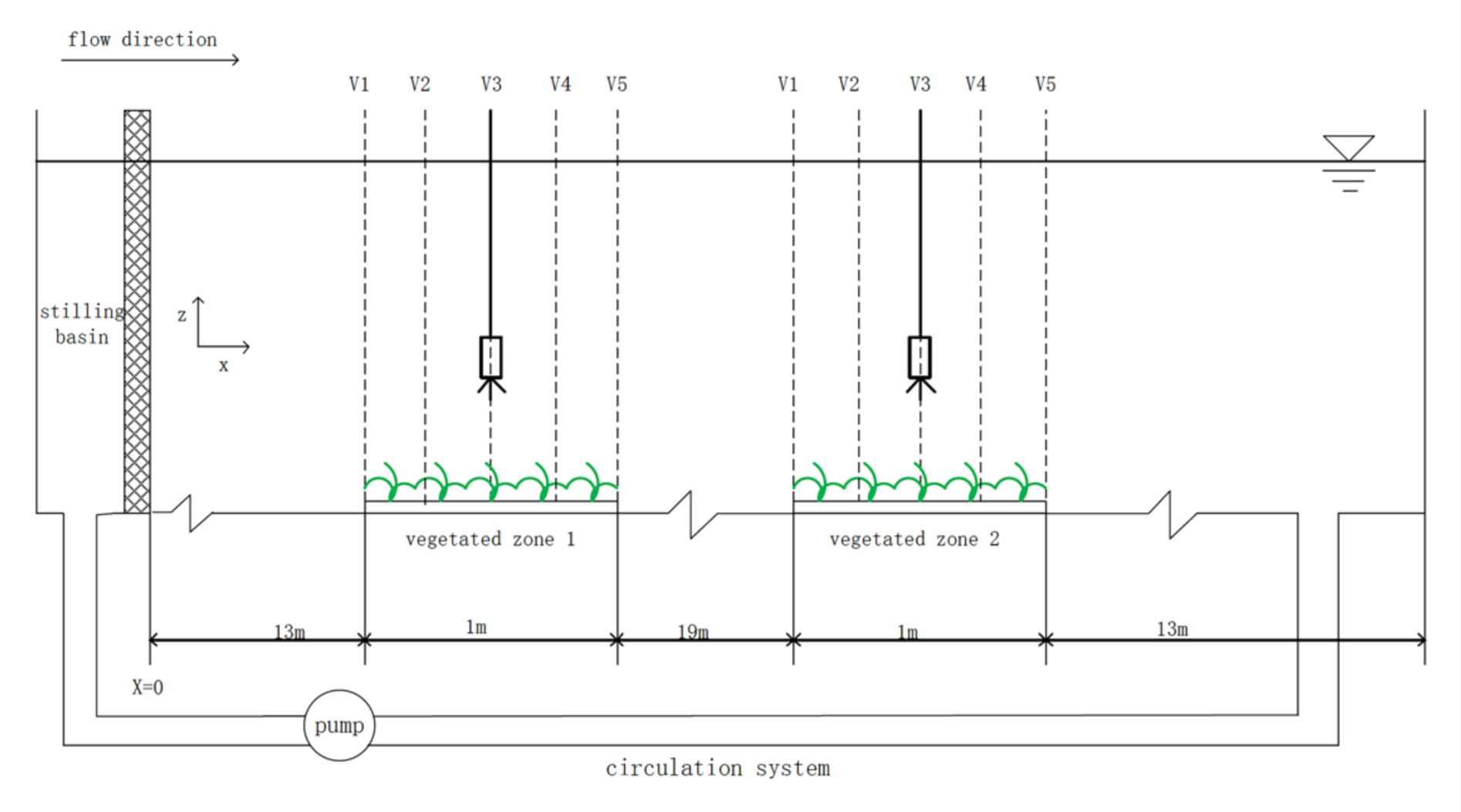
Currently, indoor flume drainage experiments are mostly used to study the flow resistance of vegetation. In this paper, all the experiments were conducted at the International Research Center for Coastal and Offshore Engineering of Zhejiang University. The experiment device (Figure 1) includes a rectangular water tank, a pressure gauge, a tailgate, and an electromagnetic flow meter. The bottom of the tank and both walls were made of Plexiglas. As shown in Figure 1, the tank was 47 m long, 0.6 m wide, and 0.8 m deep. The circulation of currents was ensured by the underground circulation system during the experiment. Model vegetation was planted at two different places. The length of the planted zone is 1 m, with one between 13 and 14 m, and the other between 33 and 34 m from the beginning of the channel.
The Acoustic Doppler Velocimeter (ADV) manufactured by Son Tek Inc., (San Diego, CA, USA) was used to measure the flow characteristics. The pulse-to-pulse coherent measuring method is the basis of the ADV technology. Three modules are concluded in this instrument: a measuring probe, a conditional module, and a module that can do the processing. The sampling volume (approximately 0.125 cm3) is 5 cm from the sensing elements, and it can measure mean velocity and velocity fluctuation. Via a processing card, the probe was connected to the computer [11]. Real-time data could be recorded using a data acquisition program installed in the sampling computer.
The ADV was mounted in a metal frame of each test area. In addition, it could be easily moved upstream and downstream ensuring that all the measurements were vertically aligned. The components of velocity, , , and correspond to the streamwise (), lateral (), and vertical () directions, respectively. During the current propagation, the ADV was utilized at a sampling frequency of 25 Hz with a 60 s sampling time [7]. Thus, 1500 data samples were acquired to estimate the average value for each measurement point. However, owing to ADV limitations, measurements cannot be taken in the region 50 mm below the water’s surface.
Additionally, for purpose of avoiding spikes during the velocity record, the data recorded by ADV was adopted only when the signal-to-noise ratio (SNR) was greater than 15 dB, and the correlation (COR) was greater than 70% [30,31]. The acceleration threshold method in [32] was used to remove spikes. In order to ensure the repeatability and accuracy of the experiment, all tests were carried out at least twice. If the despiked results of two groups were similar, the average values were adopted to do further analysis; otherwise, the experiment was repeated until achieving the appropriate results.
In order to filter and post-process the sampled data, a post-processing program, the Win-ADV program was used. Data with an average correlation equal to or less than 70% were filtered out [11]. The Win-ADV-program, a post-processing program, was used to filter and post-process the sampled data [33]. Special care is needed when interpreting ADV measurements. The Doppler noise can greatly alter the true turbulence characteristics, even for high-turbulence flows [32]. Other sources of error include low SNR, measuring time, and probe orientation.
2.2. Vegetation Material
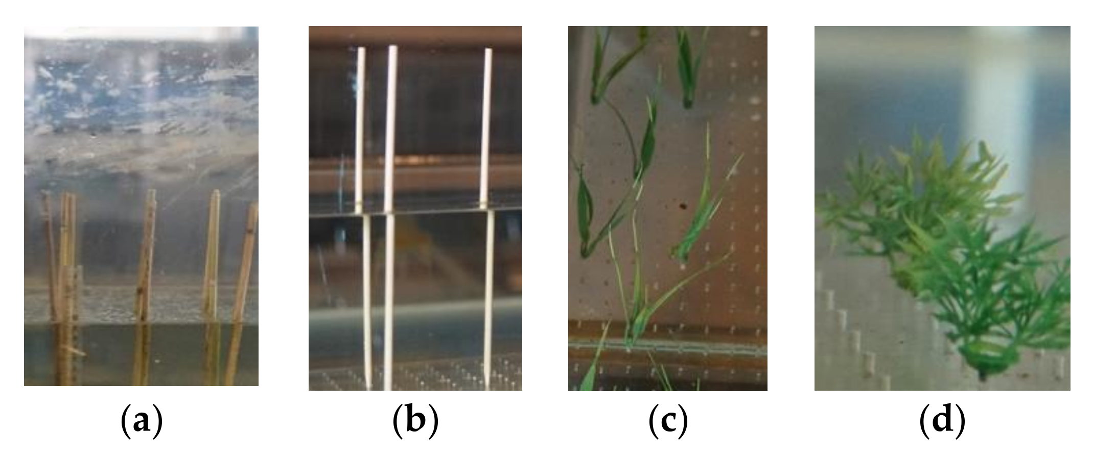
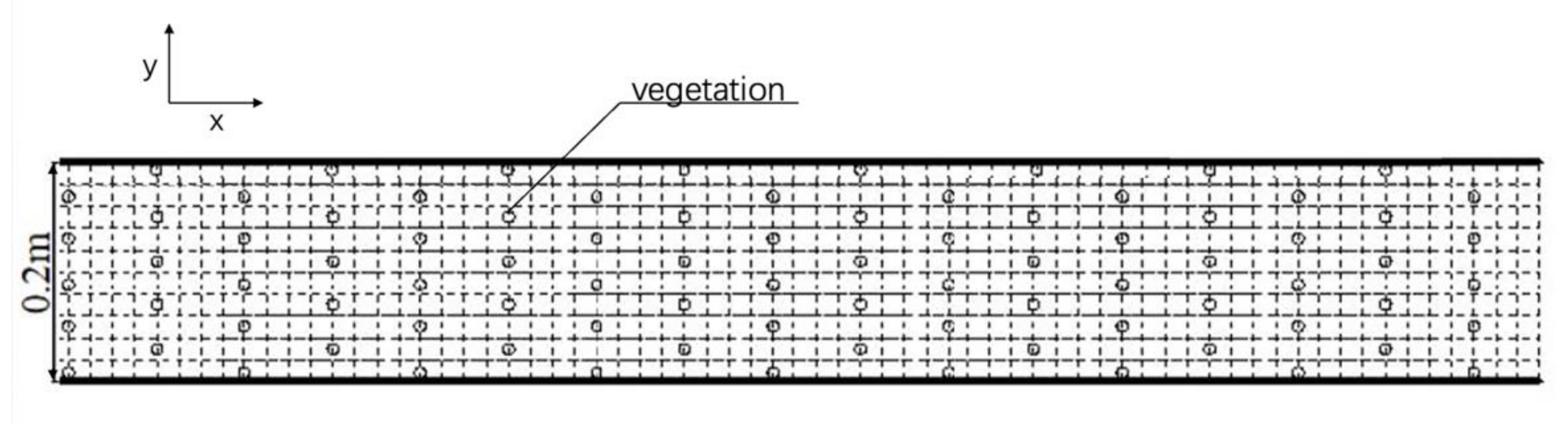
To present four different vegetations on the floodplain, the researchers chose reeds and wooden sticks as rigid submerged plants, and plastic grass and chlorella as flexible emerged plants, respectively, which are shown in Figure 2. The reed and wooden stick (Figure 2a,b) were 30 cm in length and had a radius of 0.8 cm, while the height of the grass (Figure 2c) was 10 cm and the height of chlorella (Figure 2d) was 5–6 cm. The experimenter placed the mimic vegetation by putting various plants in the prepared holes drilled in the PVC board with dimensions of 1 × 0.2 × 0.005 m (length, width, and thickness), ignoring swaying and bending. For each type of vegetation, the pattern and the density are the same. The distance of two plants along the direction is 8 cm, the distance of plants along the direction is 4 cm. Thus, the density of vegetation is 200 stems/m2 and the top view of the vegetation can be seen in Figure 3.
2.3. Experiment Method
Previous researchers have used the traditional flume method to study the flow characteristics of different plants, with only one plant being measured at a time. However, the multi-group synchronous experiment flume method was innovatively proposed by the authors, which means that researchers can carry out multiple simultaneous tests instead of one. During one test, for instance, as is shown in Figure 1, two different types of vegetation can be placed on the Vegetated Zone 1 and Vegetated Zone 2, respectively. Therefore, this proposed method can control the same flow conditions and the results have better contrast. In addition, this method can save the test cost and greatly improves the test efficiency.
2.4. Experimental Conditions
In this experiment, at the beginning of the test area, a set of three flow depths h (0.15, 0.2, 0.25 m) and five discharges Q (10, 15, 20, 25, 30 L/s) were adopted (Table 1). The slope of the flume was fixed at 0.0015%. In addition, according to the Applied Hydromechanics [34], the Reynold Number and the Froude Number in Table 1 were defined by Equations (1) and (2), respectively.
where represents the velocity, represents the hydraulic radius, represents the kinematic viscosity, represents the acceleration due to gravity, and represents the water depth.
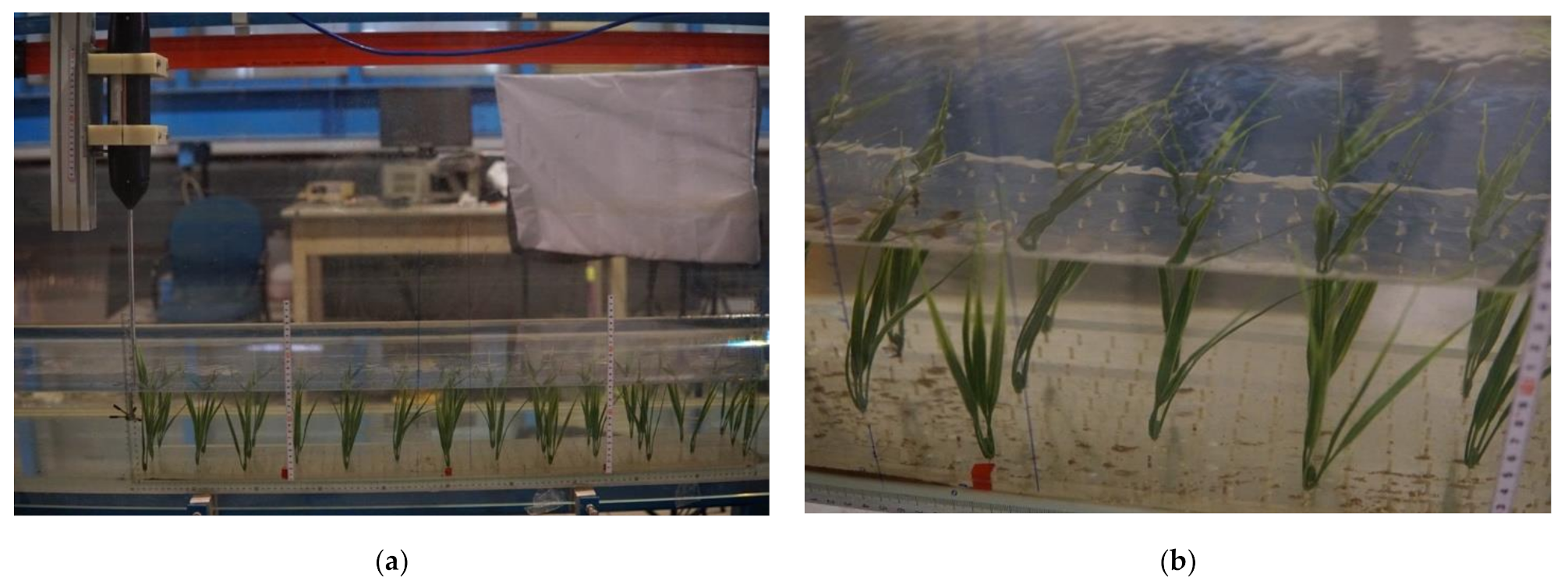
It is fully recognized that, although the size and scale of the experiment flume and experimental setup are small, albeit with small Reynolds numbers, the data can make sense under turbulent flow conditions. Regardless of scale, the structure of turbulence intensity is similar in nature. In addition, in the past, laboratory experiments were the sole effective way to obtain adequate data on both temporal and spatial scales. Such data obtained in a laboratory have often been directly applicable at full scale [35]. In addition, one example is presented in Figure 4, showing the distinctly different performance of grass when the velocity varies.
2.5. Locations of Flow Measurement
Figure 1 shows that the authors arranged two plant layout belts named Vegetated Zone 1 and Vegetated Zone 2. Both of them are of length of 1 m and width of 0.2 m. Five measurement verticals are set equidistant on each belt from the beginning of each vegetated zone, which are denoted as vertical 1, vertical 2, vertical 3, vertical 4, and vertical 5, respectively (V1, V2, V3, V4, and V5). Therefore, we measured the velocity distributions and the flow depth at five verticals of each vegetated belt to investigate the flow characteristics.
Data for four different types of vegetations, have been tested in this research. A summary of experimental conditions is presented in Table 1. For all the tests, the Reynolds numbers, Re, ranged from approximately 9068–33,200, which indicates that they are within the range of turbulence flow. In addition, the Froude numbers, Fr, ranged from 0.0018–0.0754, meaning that they can be considered subcritical flow.
3. Analytical Method
3.1. Mean Velocity
3.2. Turbulence Intensity
Analysis was carried out based on measurements of velocity fluctuations at one point in the flow. In this research, both the mean flow velocity elements (, , ) and velocity fluctuation components in turbulence (, , ) correspond to the streamwise, lateral, and vertical directions, respectively. Velocity fluctuations can be regarded as the deviation from the mean velocity. In general, root-mean-square (RMS) of velocity fluctuation is considered to be a measure of turbulence intensity. Turbulence intensities corresponding to three different directions: streamwise, lateral, and vertical directions are defined as follows:
where is the total number of observations in a given sequence; , , and are velocity fluctuations of streamwise, lateral, and vertical flow, respectively; , , and are turbulence intensities corresponding to streamwise, lateral, and vertical flow, respectively [7].
3.3. Flow Resistance Coefficient
It is of great significance to estimate the flow resistance effected by vegetation in river and coastal management because of its potentially important effects on channel conveyance. Efforts to quantify hydraulic roughness in vegetated channels date from the 1950s to 1960s. During the 1950s to 1960s, researchers take efforts to quantify hydraulic roughness in vegetation planted channels. Lots of methods were proposed based on the drag force equation for quantifying resistance ranging from one-dimensional approaches (e.g., Manning coefficient or Darcy-Weisbach friction) to three-dimensional approaches. Järvelä, J [8] used measured head losses to estimate the Darcy-Weisbach friction coefficient. In practice, the most widely used approach is the Manning coefficient , the quantifying metric in vegetation density, river hydraulics, plant frontal area, and vegetation stiffness. Flow resistance is mainly determined by vegetation. In addition, researchers used the vegetation drag coefficient as a fitting parameter. In this study, the Manning coefficient is calculated using Equation (7) proposed by Fischenich [36,37].
where represents the hydraulic radius; is the bulk drag coefficient; is the vegetation density per unit channel length; and is the dimensional conversion factor. The empirical formula Equation (8) for calculating for emerged and submerged vegetation resistance coefficient is as follows [38]:
where represents the volume fraction of the vegetation, represents the velocity; represents the characteristic length; represents the kinematic viscosity. Therefore, we can calculate with these equations.
4. Results and Discussions
4.1. Mean Velocity Profiles
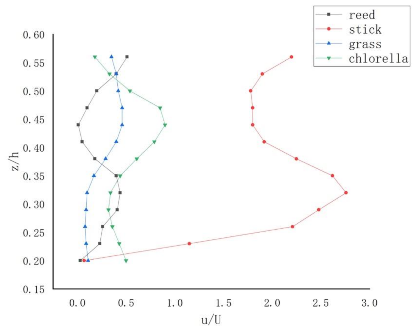
Velocities at one point can be measured in three mutually perpendicular directions: streamwise (, parallel to the boundary), lateral (, normal to the boundary), and vertical (). Thus, researchers use several test runs to investigate the flow velocities and turbulence intensity, respectively, in x, y, and z directions. Figure 5 presents the measured velocity patterns on the plane against , where is the vertical length from the bed, is the water depth and means the shear velocity, calculated by the equation , in which is the energy slope [11].
Figure 5 represents the vertical distribution of the time-averaged velocities at vertical 4 when Q is 20 L/s. It represents that the mean flow after vegetation is planted is obviously slower and does not follow a logarithmic distribution anymore.
Obviously, this is different among four different vegetations. Firstly, as submerged rigid vegetation, both reed and wooden stick follows the s-shape. However, as merged flexible vegetations, grass and chlorella follow the opposite of the s-shape. Therefore, the shape of the profile may depend on the type of vegetation. Figure 5 also presents that the relationship between the height of a plant and the water depth influences the distribution of vertical velocity. Furthermore, they vary significantly in mean velocity distributions and exhibit the formation of a horizontal shear layer. The magnitude of the mean velocity for the wooden stick is more than others because the wooden stick consumes much less energy and momentum from the flow through the generation of turbulence. This result is similar to the paper by [35]. In Yang’s 2007 study, three zones were divided by the s-shape pattern and the degree of each region was related to flow depth and vegetation type [35]. For the rigid vegetation river course, the resistance of plants after planting reduces the mean velocity of water flow, and the velocity of the section is redistributed. The velocity of the plant area does not obey the logarithmic distribution law anymore, and the velocity distribution of each section is different. Current velocity stratification is not obvious. For the grass and chlorella, the distributions of point velocity show a reversed s-shape (Figure 5). For the flexible vegetation channel, the vegetation fluctuation and deflection phenomenon make the water flow unstable and the vertical flow velocity decreases. The vegetation curve streamlines and fluctuates obviously, and the top of the vegetation layer has a tendency to be flattened by water. In particular, the velocity distribution of grass near the top area of the vegetation layer presents a semilogarithmic distribution. In the inner area near the bottom of the tank, the longitudinal velocity is very small due to the obstruction of the water flow by the aquatic plants, but the velocity distribution in the vertical direction from the bottom of the channel to the top of the vegetation layer always increases, and after reaching the top of the vegetation layer, the friction consumes a lot of momentum. Due to the existence of viscous shear stress between liquids, the flow in this region is moved forward by the drag force of the upper fluid, so the flow velocity keeps increasing until it reaches a certain height and the flow velocity increases to a certain value until it basically returns to stability. After stability, the flow velocity distribution still follows the semilogarithmic relationship.
4.2. Turbulence Intensities
The transportation and settlement of sediment in the river course, the erosion of the riverbed embankment, and the resistance of flow are all affected by the flow turbulence. With the increasing maturity and perfection of three-dimensional turbulence numerical simulation, it is very important to verify these models with high-quality test data. Therefore, it is significant to study the flow turbulence intensity.
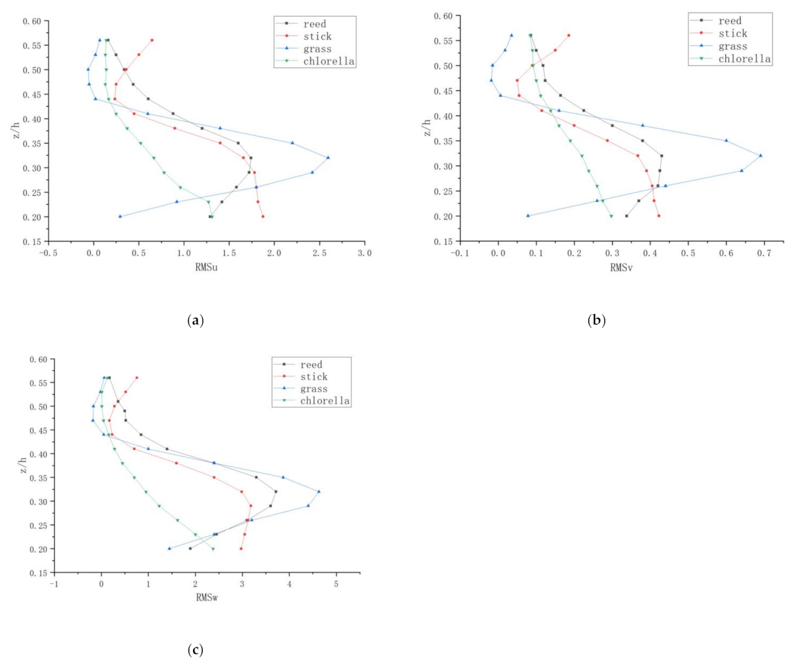
Figure 6 shows the distribution of turbulence intensities,, and against the relative depth at the vertical 5 (V5) of different vegetations with Q = 30 L/s. These changes correspond to the vertical distribution of velocity along the flow points. In the case of a vegetative floodplain, the vertical distribution of turbulence intensity along with the flow and transverse turbulence intensity are also s-shaped. However, the type of vertical turbulence intensity distributions in each direction are not the same kind. The phenomenon where the streamwise and lateral intensities are approximately equal by comparing the distribution in three different directions was found.
According to Figure 6, in the water near the surface part, the three directions of longitudinal, lateral, and vertical, turbulence intensity is bigger and it may be that the interaction of water and plants produces a turbulent vortex and interface wave. There is a strong momentum exchange here, and somewhere in the region a maximum is reached, then near the surface it decreases. Figure 6 also shows that the turbulence intensity distribution is anisotropic.
It can also be analyzed from the figure that the vertical turbulence intensity and turbulence intensity distribution law of vertical and horizontal difference is bigger, and vertical turbulence intensity is less than streamwise and lateral, which is due to the turbulent vortex in the statistical measure of vertical being less than the horizontal scale of turbulence which did not reach isotropic. Maybe it is due to the measurements being from the outer layer.
For the river course with rigid vegetation, the turbulence intensity in the three directions near the water surface is larger and reaches the maximum in this area, while it decreases at the area near the water surface. Turbulence is not isotropic. The change law of turbulence intensity is different in different sections. For the channel with flexible vegetation, strong mass and momentum exchange exists at the top of the planted area, and the turbulence intensity is relatively large in the streamwise, spanwise and vertical directions, respectively. As the statistical scale of the turbulent vortex in the vertical direction is obviously smaller than that in the horizontal direction, the turbulence does not reach isotropy. The change law of turbulence intensity is also different in different sections. This is consistent with the distribution law of turbulence intensity in the river channel with rigid vegetation.
4.3. Reynold Stress
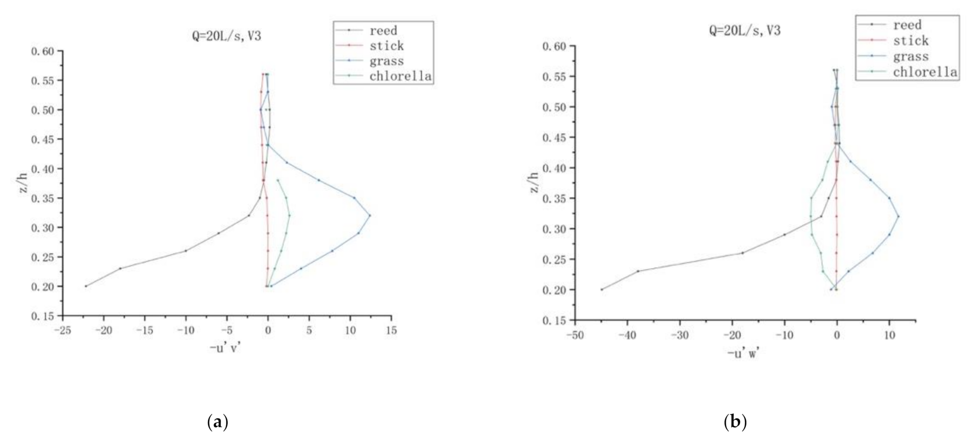
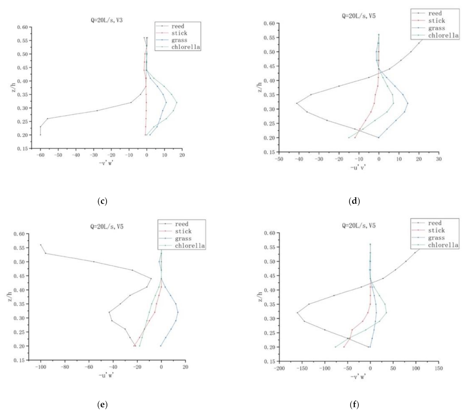
By using the equation , the Reynold shear stresses can be calculated from the raw turbulent data [7]. For the purpose of determining the effects of various vegetations on Reynolds stress distribution, the profiles of Reynolds stresses , , and against the relative depth at two different verticals, vertical 3 (V3) and vertical 5 (V5) of four different vegetations, is presented in Figure 7.
At vertical 3, when the discharge is 20 L/s, wide variations of the and exist when the z/h is between 0.44 and 0.56. The change is most obvious in reed. The figures demonstrate the Reynold stresses of all these four vegetations show anisotropy. The values of reed and chlorella varied the most, and the values of chlorella varied the least, which might be caused by the difference of the submergence mode and flexibility between reed and chlorella.
The Reynold stress for reed reaches a maximum when the z/h is 0.2. However, the Reynold stress for stick is approximately near zero. Nevertheless, these magnitudes are relatively smaller than those at other positions owing that the flow is not markedly affected by plants. For grass and chlorella, they reached the maximum when z/h was 0.32, with the maximum of Reynold stress for grass being larger than chlorella. When the relative height was greater than 0.44, the Reynolds stress of the four plants in three directions was roughly the same. The Reynolds stress of reed was the largest. However, the Reynolds stress on the wooden stick was almost zero. Both reeds and sticks are stiff plants, but the Reynolds stress varies greatly, possibly because of the composition of their plants. For submerged flexible plants, the Reynolds stress of aquatic plants in both directions is greater than that of chlorella, which may be due to their different heights. This phenomenon shows that the turbulent transport of momentum of the wooden stick is so little that the Reynold stress can be neglected. However, at vertical 5, the profile of reed varied while the values of stick, grass, and chlorella was still near zero.
Therefore, the Reynolds stress has a large value in the zone close to the water surface and riverbed floor, and reaches the maximum in each area, indicating that there is a strong shear action between the water bodies in this area. In the region of 0.2 to 0.4 relative height, the Reynolds stress is relatively small. Generally speaking, the Reynolds stress in the upper part of the submerged vegetation layer is greater than that in the lower part, which is conducive to the deposition of cohesive sediment, which is also one of the root causes of the vegetation revetment.
In addition, the distribution of Reynolds stress of each vertical line is different. This is due to the structural differences among plants, that is, the water blocking zone of vegetations and the physical resistance of them, as well as the complex “tree group” effect among plants, which makes the Reynolds stress distribution at different survey line positions different.
It can also be seen from the figure that, from the bottom to the top of the vegetation layer, the longitudinal, transverse, and vertical Reynolds stress varies in different sections. In the upper part of the vegetation, Reynolds stress has a large value when z/h reaches a certain value, respectively, which may be related to the shape of the vegetation itself and the vegetation arrangement before and after the section, so that the flow patterns at each section are different.
For the river course with rigid vegetation, the Reynolds stress has a large value near the water surface and reaches the maximum value somewhere in the region, indicating that there is a strong shear between water bodies in this region. The Reynolds stress decreases in this region. Generally speaking, the Reynolds stress in the upper part of the vegetation layer flooded by water is greater than that in the lower part, which is conducive to the deposition of viscous sediment, which is also one of the root causes of the vegetation revetment. The Reynolds stress varies in different sections.
For the river course with flexible vegetation, due to the difference in the shape of the vegetation itself and the arrangement of vegetation before and after the section, the change rule of Reynolds stress variable at each section is different, and the flow pattern is also different. A strong shearing effect exists on the top of the vegetation layer and the upper water body, with the Reynolds stress reaching the maximum value near the top of the vegetation layer. From the top down, the Reynolds stress decreases. The sheer velocity of the water flow at the bottom of the vegetation layer, namely, the Reynolds stress, decreases, which is the same as that in the case of rigid vegetation.
Therefore, although the water flow phenomena observed in rigid plants and flexible plants are different, there are many similarities in their hydraulic characteristics, and some laws are basically the same.
4.4. Manning Coefficient
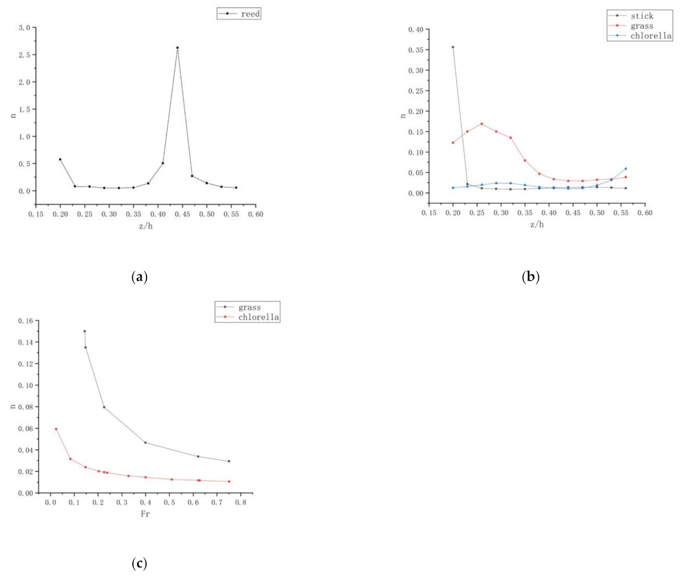
This paper used the Manning Coefficient in order to calculate the flow resistance affected by different types of vegetation. The sidewall and vegetation bottom resistance ( and ) are included in the total flume resistance [11]. However, these two kinds of resistances can be negligible compared to that of vegetation because the flume wall is made of glass. In other words, the resistance of the vegetation bottom is dominant in the flow resistance in a planted flume. The authors applied Equation (2) to deduce the flow resistance . After careful studying of various test runs, Figure 8 shows how the Manning coefficient changes with the relative water depth , the vegetation type, and the Froude numbers.
Figure 8a,b represents how the Manning coefficient for different vegetations varies when the relative depth differs. As is shown in the figure, the resistance of flow varies with the vegetation types, with grass retarding the flow the most. Figure 8a shows that the general trend for reed is an increase in the Manning Coefficient value n with increasing relative depth, z/h, on the occasion of z/h < 0.45. The value reached a maximum when z/h is 0.45. Conversely, when z/h > 0.45, the Manning coefficient decreases with increasing the relative depth. In addition, both reed and wooden stick, as merged rigid vegetations, have similar average values of n.
Moreover, it is so different in the submerged flexible vegetations. The Manning coefficient of grass is still larger than the value of chlorella. The two vegetations have different heights, so they have different influences on flow. The flow resistance is different. Furthermore, the mean value of the Manning coefficient for submerged flexible vegetations is less than that of merged stiff vegetations, presenting that the type of vegetation is the key point of the flow resistance. Therefore, it is significant for scientists to research the flow resistance of each vegetation.
Figure 8 indicates that the Manning coefficient of grass and chlorella decreases with increasing . The Manning coefficient of grass is larger than that of chlorella, showing that different vegetations differ in flow resistance. When is 0.1, the Manning coefficient for grass is approximately 0.15, which is six times as much as the Manning coefficient for chlorella. Therefore, the water depth and the type of vegetation are the crucial factors significantly influencing the Manning coefficient .
5. Conclusions
These small-scale experiments reported that the distribution of streamwise mean velocity for emerged rigid vegetation follows an s-shape curve that exhibits three regions, different for the various types of vegetation, as shown in Figure 5. The resistance of flow varies with the vegetation type, with long grass retarding the flow the most (Figure 8). The lateral gradient of velocity increases after the floodplain is vegetated, thereby increasing the apparent shear stress on the vertical interface.
The vertical distributions of streamwise and lateral turbulence intensities are s-shaped for vegetated floodplains, similar to the distributions of streamwise point velocity. The turbulence intensity, however, does not follow the same kind of distribution. The streamwise and lateral turbulence intensities are approximately equal. The vertical turbulence intensity is the weakest. The vegetation on the floodplain affects the spatial distribution of Reynold stresses. For vegetated cases, although the water flow phenomena observed by rigid plants and flexible plants are different, there are many similarities in their hydraulic characteristics, and some laws are basically the same.
This work focuses on a single density of four different aquatic plants in a riparian zone only under the current. Further studies should pay attention to investigate the wave-current flows in the canopy with vertically varying density. For further investigations, several low depths and flow rates can be adopted to investigate variations of flow fields altered by different configurations. In addition, more plant clumps and measurement positions in the streamwise direction should be added to thoroughly study these variations. As the high variations of flow fields occur at the sheath section and around the vegetation top, a small measured interval is suggested to accurately capture the maximum Reynold stress and velocity.
Based on the experimental work, a better understanding of flow resistance due to different types of natural stiff and flexible vegetation under merged and submerged vegetation can be derived from the data. In addition, the data can be applied to numerical models. Furthermore, the experiments on natural plants also provide a powerful reference basis for other investigations utilizing artificial vegetation. In the next phase of analysis, velocity distributions and turbulence within and above the vegetation layer will be reported in more detail.
Author Contributions
Conceptualization, X.M. and Y.Z.; methodology, X.M.; formal analysis, K.D.; writing—original draft preparation, X.M. and Y.Z.; writing—review and editing, X.M. and Y.Z.; supervision, L.C.; supervision, Z.S. All authors have read and agreed to the published version of the manuscript.
Funding
This research received no funding.
Institutional Review Board Statement
Not applicable.
Informed Consent Statement
Not applicable.
Data Availability Statement
Not applicable.
Acknowledgments
We are grateful to the International Research Center for Coastal and Offshore Engineering, Zhejiang University, for the use of the laboratory facilities, and to Jiayun Zheng, Yunze Shen, and Fanjun Chen for help on this research.
Conflicts of Interest
The authors declare no conflict of interest.
References
- Szabo-Meszaros, M.; Navaratnam, C.U.; Aberle, J.; Silva, A.T.; Forseth, T.; Calles, O.; Fjeldstad, H.P.; Alfredsen, K. Experimental hydraulics on fish-friendly trash-racks: An ecological approach. Ecol. Eng. 2018, 113, 11–20. [Google Scholar] [CrossRef]
- Sonnenwald, F.; Guymer, I.; Stovin, V. A CFD-Based Mixing Model for Vegetated Flows. Water Resour. Res. 2019, 55. [Google Scholar] [CrossRef] [Green Version]
- Zhang, Y.; Tang, C.; Nepf, H. Turbulent Kinetic Energy in Submerged Model Canopies under Oscillatory Flow. Water Resour. Res. 2018, 54, 1734–1750. [Google Scholar] [CrossRef]
- Li, D.; Huai, W.-X.; Liu, M.-Y. Investigation of the flow characteristics with one-line emergent canopy patches in open channel. J. Hydrol. 2020, 590, 125248. [Google Scholar] [CrossRef]
- Leonard, L.A.; Luther, M.E. Flow hydrodynamics in tidal marsh canopies. Limnol. Oceanogr. 1995, 40, 1474–1484. [Google Scholar] [CrossRef]
- Kemp, J.L.; Harper, D.M.; Crosa, G.A. The habitat-scale ecohydraulics of rivers. Ecol. Eng. 2000, 16, 17–29. [Google Scholar] [CrossRef]
- Chen, S.C.; Kuo, Y.M.; Li, Y.H. Flow characteristics within different configurations of submerged flexible vegetation. J. Hydrol. 2011, 398, 124–134. [Google Scholar] [CrossRef]
- Järvelä, J. Flow resistance of flexible and stiff vegetation: A flume study with natural plants. J. Hydrol. 2002, 269, 44–54. [Google Scholar] [CrossRef]
- Järvelä, J. Effect of submerged flexible vegetation on flow structure and resistance. J. Hydrol. 2005, 307, 233–241. [Google Scholar] [CrossRef]
- Stephan, U.; Gutknecht, D. Hydraulic resistance of submerged flexible vegetation. J. Hydrol. 2002, 269, 27–43. [Google Scholar] [CrossRef]
- Xia, J.; Nehal, L. Hydraulic features of flow through emergent bending aquatic vegetation in the riparian zone. Water 2013, 5, 2080–2093. [Google Scholar] [CrossRef]
- Zhang, S.; Li, G.; He, X.; Liu, Y.; Wang, Z. Water flow resistance characteristics of double-layer vegetation in different submerged states. Water Sci. Technol. Water Supply 2019, 19, 2435–2442. [Google Scholar] [CrossRef]
- Weltz, M.A.; Arslan, A.B.; Lane, L.J. Hydraulic Roughness Coefficients for Native Rangelands. J. Irrig. Drain. Eng. 1992, 118, 776–790. [Google Scholar] [CrossRef] [Green Version]
- Hu, S.; Abrahams, A.D. Resistance to overland flow due to bed-load transport on plane mobile beds. Earth Surf. Process. Landf. 2004, 29, 1691–1701. [Google Scholar] [CrossRef]
- Hu, S.; Abrahams, A.D. The effect of bed mobility on resistance to overland flow. Earth Surf. Process. Landf. 2005, 30, 1461–1470. [Google Scholar] [CrossRef]
- Hu, S.; Abrahams, A.D. Partitioning resistance to overland flow on rough mobile beds. Earth Surf. Process. Landf. 2006, 31, 1280–1291. [Google Scholar] [CrossRef]
- Liu, Y.; Xu, J.; Zhou, G. Relation between crack propagation and internal damage in sandstone during shear failure. J. Geophys. Eng. 2018, 15, 2104–2109. [Google Scholar] [CrossRef] [Green Version]
- Ferro, V. Assessing flow resistance law in vegetated channels by dimensional analysis and self-similarity. Flow Meas. Instrum. 2019, 69, 101610. [Google Scholar] [CrossRef]
- Guillén-Ludeña, S.; Lopez, D.; Mignot, E.; Riviere, N. Flow Resistance for a Varying Density of Obstacles on Smooth and Rough Beds. J. Hydraul. Eng. 2020, 146. [Google Scholar] [CrossRef]
- Bialik, R.J.; Karpiński, M.; Rajwa, A.; Luks, B.; Rowiński, P. łM Bedform characteristics in natural and regulated channels: A comparative field study on the Wilga River, Poland. Acta Geophys. 2014, 62, 1413–1434. [Google Scholar] [CrossRef]
- Parsons, D.R.; Best, J.L.; Orfeo, O.; Hardy, R.J.; Kostaschuk, R.; Lane, S.N. Morphology and flow fields of three-dimensional dunes, Rio Paraná, Argentina: Results from simultaneous multibeam echo sounding and acoustic Doppler current profiling. J. Geophys. Res. Earth Surf. 2005, 110, 1–9. [Google Scholar] [CrossRef] [Green Version]
- Shugar, D.H.; Kostaschuk, R.; Best, J.L.; Parsons, D.R.; Lane, S.N.; Orfeo, O.; Hardy, R.J. On the relationship between flow and suspended sediment transport over the crest of a sand dune, Río Paraná, Argentina. Sedimentology 2010, 57, 252–272. [Google Scholar] [CrossRef]
- Defina, A.; Bixio, A.C. Mean flow and turbulence in vegetated open channel flow. Water Resour. Res. 2005, 41, 1–12. [Google Scholar] [CrossRef] [Green Version]
- Hui, E.Q.; Hu, X.E.; Jiang, C.B.; Ma, F.K.; Zhu, Z.D. A study of drag coefficient related with vegetation based on the flume experiment. J. Hydrodyn. 2010, 22, 329–337. [Google Scholar] [CrossRef]
- Busari, A.O.; Li, C.W. Bulk drag of a regular array of emergent blade-type vegetation stems under gradually varied flow. J. Hydro Environ. Res. 2016, 12, 59–69. [Google Scholar] [CrossRef]
- Parsons, A.J.; Abrahams, A.D.; Wainwright, J. On determining resistance to interrill overland flow. Water Resour. Res. 1994, 30, 3515–3521. [Google Scholar] [CrossRef]
- Mu, H.; Yu, X.; Fu, S.; Yu, B.; Liu, Y.; Zhang, G. Effect of stem basal cover on the sediment transport capacity of overland flows. Geoderma 2019, 337, 384–393. [Google Scholar] [CrossRef]
- Sun, Z.L.; Zheng, J.Y.; Zhu, L.L.; Chong, L.; Liu, J.; Luo, J.Y. Influence of submerged vegetation on flow structure and sediment deposition. J. Zhejiang Univ. (Eng. Sci.) 2021, 55, 71–80. [Google Scholar] [CrossRef]
- Zhang, S.; Wang, Z.; Liu, Y.; Li, G.; Chen, S.; Liu, M. The influence of combined vegetation stalk thickness on water flow resistance. Water Environ. J. 2019, 34, 455–463. [Google Scholar] [CrossRef]
- Chen, M.; Lou, S.; Liu, S.; Ma, G.; Liu, H.; Zhong, G.; Zhang, H. Velocity and turbulence affected by submerged rigid vegetation under waves, currents and combined wave–current flows. Coast. Eng. 2020, 159. [Google Scholar] [CrossRef]
- Carollo, F.G.; Ferro, V.; Termini, D. Analyzing Turbulence Intensity in Gravel Bed Channels. J. Hydraul. Eng. 2005, 131, 1050–1061. [Google Scholar] [CrossRef]
- Goring, D.G.; Nikora, V.I. Despiking Acoustic Doppler Velocimeter Data. J. Hydraul. Eng. 2002, 128, 117–126. [Google Scholar] [CrossRef] [Green Version]
- Wahl, T.L. Analyzing ADV data using WinADV. Jt. Conf. Water Resour. Eng. Water Resour. Plan. Manag. 2000 Build. Partnerships 2004, 104, 1–10. [Google Scholar] [CrossRef] [Green Version]
- Hydromechanics, A. Engineering Course: Applied Hydromechanics. 2020. [Google Scholar]
- Yang, K.; Cao, S.; Knight, D.W. Flow Patterns in Compound Channels with Vegetated Floodplains. J. Hydraul. Eng. 2007, 133, 148–159. [Google Scholar] [CrossRef]
- Fischenich, C. Resistance Due to Vegetation. Ecosyst. Manag. Restorat. Res. Progr. 2000, 37, 1–9. [Google Scholar]
- Fischenich, C.; Dudley, S. Determining drag coefficients and area for vegetation. Ecosyst. Manag. Restorat. Res. Progr. 1999, 2, 36. [Google Scholar]
- Wang, W.J.; Peng, W.Q.; Huai, W.X.; Katul, G.G.; Liu, X.B.; Qu, X.D.; Dong, F. Friction factor for turbulent open channel flow covered by vegetation. Sci. Rep. 2019, 9, 1–16. [Google Scholar] [CrossRef]
Figure 1.
Experimental setup: schematic of the flume (long view, not to scale).

Figure 2.
Different types of vegetation: (a) reed, (b) stick, (c) grass, (d) chlorella.

Figure 3.
Top view of the vegetation.

Figure 4.
Test run S9 with grasses. (a) The average flow velocity is 0. (b) The average flow velocity is 0.23 m/s.
Figure 4.
Test run S9 with grasses. (a) The average flow velocity is 0. (b) The average flow velocity is 0.23 m/s.

Figure 5.
Vertical distributions of point velocity at vertical 4 with Q = 20 L/s for different vegetations: reed and stick at the length of 30 cm, grass at the length of 10 cm, and the chlorella at the length of 5–6 cm.
Figure 5.
Vertical distributions of point velocity at vertical 4 with Q = 20 L/s for different vegetations: reed and stick at the length of 30 cm, grass at the length of 10 cm, and the chlorella at the length of 5–6 cm.

Figure 6.
Vertical distributions of , and at the vertical 5 with Q = 30 L/s for different vegetations: reed and stick at the length of 30 cm, grass at the length of 10 cm, and the chlorella at the length of 5–6 cm. (a) Vertical distributions of ; (b) Vertical distributions of ; (c) Vertical distributions of .

Figure 7.
Vertical distributions of , and at verticals 3 and 5, respectively, with Q = 20 L/s for four different vegetations: reed and stick at the length of 30 cm, grass at the length of 10 cm, and the chlorella at the length of 5–6 cm: (a) Vertical distributions of at verticals 3 with Q = 20 L/s; (b) Vertical distributions of at verticals 3 with Q = 20 L/s; (c) Vertical distributions of at verticals 3 with Q = 20 L/s; (d) Vertical distributions of at verticals 5 with Q = 20 L/s; (e) Vertical distributions of at verticals 5 with Q = 20 L/s; (f) Vertical distributions of at verticals 5 with Q = 20 L/s.


Figure 8.
Manning coefficient n for various vegetations: (a,b): n against relative depth, z/h, where z is the height if measurement location, h is the water depth; (c) n against the Froude number, Fr.
Figure 8.
Manning coefficient n for various vegetations: (a,b): n against relative depth, z/h, where z is the height if measurement location, h is the water depth; (c) n against the Froude number, Fr.


Table 1.
Summary of experimental conditions.
| Scheme | Data Number | H (cm) | Discharge (L/s) | Vegetation | Re | Fr | |
|---|---|---|---|---|---|---|---|
| S1 | Run01 | 15 | 10.00 | reed | stick | 10,967 | 0.0082 |
| S2 | Run02 | 15 | 10.00 | grass | chlorella | 10,967 | 0.0082 |
| S3 | Run03 | 15 | 15.00 | reed | stick | 16,620 | 0.0189 |
| S4 | Run04 | 15 | 15.00 | grass | chlorella | 16,620 | 0.0189 |
| S5 | Run05 | 15 | 20.00 | reed | stick | 22,134 | 0.0335 |
| S6 | Run06 | 15 | 20.00 | grass | chlorella | 22,134 | 0.0335 |
| S7 | Run07 | 15 | 25.00 | reed | stick | 27,697 | 0.0525 |
| S8 | Run08 | 15 | 25.00 | grass | chlorella | 27,697 | 0.0525 |
| S9 | Run09 | 15 | 30.00 | reed | stick | 33,200 | 0.0754 |
| S10 | Run10 | 15 | 30.00 | grass | chlorella | 33,200 | 0.0754 |
| S11 | Run11 | 20 | 10.00 | reed | stick | 9930 | 0.0035 |
| S12 | Run12 | 20 | 10.00 | grass | chlorella | 9930 | 0.0035 |
| S13 | Run13 | 20 | 15.00 | reed | stick | 14,955 | 0.0080 |
| S14 | Run14 | 20 | 15.00 | grass | chlorella | 14,955 | 0.0080 |
| S15 | Run15 | 20 | 20.00 | reed | stick | 19,944 | 0.0142 |
| S16 | Run16 | 20 | 20.00 | grass | chlorella | 19,944 | 0.0142 |
| S17 | Run17 | 20 | 25.00 | reed | stick | 24,885 | 0.0221 |
| S18 | Run18 | 20 | 25.00 | grass | chlorella | 24,885 | 0.0221 |
| S19 | Run19 | 20 | 30.00 | reed | stick | 29,910 | 0.0319 |
| S20 | Run20 | 20 | 30.00 | grass | chlorella | 29,910 | 0.0319 |
| S21 | Run21 | 25 | 10.00 | reed | stick | 9068 | 0.0018 |
| S22 | Run22 | 25 | 10.00 | grass | chlorella | 9068 | 0.0018 |
| S23 | Run23 | 25 | 15.00 | reed | stick | 13,596 | 0.0041 |
| S24 | Run24 | 25 | 15.00 | grass | chlorella | 13,596 | 0.0041 |
| S25 | Run25 | 25 | 20.00 | reed | stick | 18,082 | 0.0072 |
| S26 | Run26 | 25 | 20.00 | grass | chlorella | 18,082 | 0.0072 |
| S27 | Run27 | 25 | 25.00 | reed | stick | 22,664 | 0.0113 |
| S28 | Run28 | 25 | 25.00 | grass | chlorella | 22,664 | 0.0113 |
| S29 | Run29 | 25 | 30.00 | reed | stick | 27,191 | 0.0163 |
| S30 | Run30 | 25 | 30.00 | grass | chlorella | 27,191 | 0.0163 |
Publisher’s Note: MDPI stays neutral with regard to jurisdictional claims in published maps and institutional affiliations. |
© 2021 by the authors. Licensee MDPI, Basel, Switzerland. This article is an open access article distributed under the terms and conditions of the Creative Commons Attribution (CC BY) license (https://creativecommons.org/licenses/by/4.0/).
Share and Cite
MDPI and ACS Style
Meng, X.; Zhou, Y.; Sun, Z.; Ding, K.; Chong, L. Hydraulic Characteristics of Emerged Rigid and Submerged Flexible Vegetations in the Riparian Zone. Water 2021, 13, 1057. https://doi.org/10.3390/w13081057
AMA Style
Meng X, Zhou Y, Sun Z, Ding K, Chong L. Hydraulic Characteristics of Emerged Rigid and Submerged Flexible Vegetations in the Riparian Zone. Water. 2021; 13(8):1057. https://doi.org/10.3390/w13081057
Chicago/Turabian StyleMeng, Xin, Yubao Zhou, Zhilin Sun, Kaixuan Ding, and Lin Chong. 2021. "Hydraulic Characteristics of Emerged Rigid and Submerged Flexible Vegetations in the Riparian Zone" Water 13, no. 8: 1057. https://doi.org/10.3390/w13081057
Note that from the first issue of 2016, this journal uses article numbers instead of page numbers. See further details here.