
Changes of Streamflow Caused by Early Start of Growing Season in Nevada, United States


1
Department of Water Resources and Environment, School of Geography and Planning, Sun Yat-Sen University, Guangzhou 510275, China
2
Department of Civil and Architectural Engineering, University of Wyoming, Laramie, WY 82071, USA
*
Author to whom correspondence should be addressed.
Water 2021, 13(8), 1067; https://doi.org/10.3390/w13081067
Submission received: 15 March 2021
/
Revised: 7 April 2021
/
Accepted: 8 April 2021
/
Published: 13 April 2021
(This article belongs to the Section Hydrology)
Abstract
:The fluctuation of streamflow in snowmelt-dominated watersheds may be an indicator of climate change. However, the relationship between the start of growing season (SOS) and the streamflow in snowmelt-dominated watersheds is not clear. In this study, we update the Coupled Hydro-Ecological Simulation System (CHESS) model by incorporating the Growing Season Index (GSI) module to estimate the start of the growing season. The updated CHESS model is then used to calculate the streamflow in the Cleve Creek, Incline Creek and Twin River watersheds located in Nevada in the United States from 1981 to 2017. This updated CHESS can be applied in any regions that are suitable for deciduous vegetation. The streamflow in the static and dynamic scheme in the three watersheds have been simulated between 1981 and 2017 with the NS of 0.52 and 0.80 in the Cleve Creek, 0.46 and 0.75 in the Incline Creek, and 0.42 and 0.70 in the Twin River watersheds, respectively. The results illustrate that the SOS have come around 3–5 weeks earlier during the last 37 years. The results illustrate a high correlation between the temperature and the timing of the SOS. Early SOS leads to a substantial increase in total annual transpiration. An increase in annual transpiration can reduce aquifer recharge and increase cumulative growing season soil moisture deficit. Comparing to the streamflow without vegetation, the streamflow with vegetation is smaller due to transpiration. As the SOS comes earlier, the peaks of the streamflow with vegetation also come earlier. If the shifts in SOS continue, the effects on annual rates of transpiration can be significant, which may reduce the risk of flooding during snowmelt. On the other hand, earlier SOS may cause soil moisture to decline during summer, which would increase the drought stress in trees and the risk of wildfires and insect infestation.
1. Introduction
The dominant form of annual precipitation in high-elevation mountains in the western United States is winter and spring snow [1,2,3]. Most of the snow accumulation in seasonal snowpack represents a natural storage reservoir [4,5]. Because most of the precipitation is concentrated in spring and winter, the western United States relies heavily on natural and man-made storage for sufficient water for agriculture, industry, and drinking during the dry summer and fall seasons [6]. Snow is a critical component of the hydrologic cycle for vegetation in the western United States and always makes the largest contribution for conifers which are photosynthetically active in the spring and early summer when meltwater is available [7]. Forest transpiration and growth are partially determined by the start of growing season (SOS) since it is limited by water availability. Hydrological models incorporating biophysical controls on forest transpiration need an accurate prediction of SOS. Process models represent snowpack as a state variable containing a mass of water that accumulates during the winter months and releases during the spring months. Since the meltwater is a vital source for generating spring runoff and re-saturating the soil to provide water for transpiration and growth, it is important to investigate the mechanisms of flow generation in snow-dominated mountain watersheds for predicting the impacts of climate change on the availability of water resources.
Previous research demonstrates the average annual temperature has increased 1–2 °C since the 1940s over western America, especially during the winter and spring seasons [8,9,10,11]. These changes have a complicated influence of climate variability on terrestrial ecosystems [12]. The worldwide warming directly influences the hydrological cycle since evapotranspiration (ET) is a critical water loss in the water balance of ecosystems [13], especially in semi-arid and arid regions [14]. Ecosystems determine streamflow quantity [15] and timing [16] by altering the ET and groundwater recharge processes [17]. Generally speaking, deforestation decreases ET and thus increases streamflow [18] and peak flow rates [19], while afforestation increases ET [20], raises shallow groundwater tables and reduces streamflow quantities [21].
It is generally assumed that warming will make SOS occur earlier in boreal and temperate ecosystems, where wintertime temperature is metabolically limiting. A simple assumption of increased primary productivity is made from the fact that more days are available for carbon assimilation and biomass growth. Several previous models have demonstrated a similar trend of the relationship between the SOS and net productivity in deciduous forests. For instance, Fu et al. [22] propose that warmer spring temperatures lead to an earlier start of net carbon uptake activity and higher spring and annual net ecosystem productivity (NEP) values in a deciduous broadleaf forest (DBF) and evergreen forest (EF). Hmimina et al. [23] illustrate that the early SOS and increasing photosynthetic activity results in a predominant greening trend over 42.0% of the vegetated area and translate to a 20.9% gain in gross primary productivity during last three decades.
However, other studies have suggested somewhat contradictory results. For example, Dunn et al. [24] find that ecosystem carbon exchange responds strongly to air temperature, moisture status, potential evapotranspiration, and summertime solar radiation. The seasonal cycle of ecosystem respiration significantly lags that of photosynthesis, limits by the rate of soil thaw and the slow drainage of the soil column. Net uptake of carbon is enhanced and respiration is inhibited by multiple years of rainfall over evaporative demand. Winchell [25] find that earlier snowmelt associated with climate warming, counterintuitively, lead to colder atmospheric temperatures during the snow ablation period and concomitantly reduce rates of net carbon uptake. Winchell concludes that when the snowmelt period occurs one month earlier than average, the forest experiences an ablation period mean air temperature of 2.7 °C, approximately 2 °C colder than an ablation period that occurs one month later than average. As most climate models project peak snow water equivalent (SWE) to occur earlier under various warming scenarios, they expect to see a decrease in total growing season carbon uptake if the post-snowmelt period is unable to compensate for the decrease in ablation period carbon uptake. Wohlfahrt et al. [26] show that reductions in the quantity and duration of daylight associated with earlier snowmelts are responsible for diminishing returns, in terms of carbon gain from early SOS.
Another uncertainty is how SOS heterogeneity affects streamflow. Streamflow may or may not increase as the regional climate warms. A common approach simulating hydrologic budgets is used for quantifying these uncertainties by dividing a heterogeneous area into smaller, more homogeneous subsites, and executing the individual model on each sub-site [27,28]. The Regional Hydro-Ecological Simulation System (RHESSys) model is built to compute a spatially varying snowpack for regional applications and is able to explicitly simulate the effects of topographic and subsurface heterogeneities on downslope redistribution of water [29]. Additionally, this model is widely used to identify saturated areas that produce runoff [30], evaluate irrigation systems [31], and examine flood potential associated with disturbances such as deforestation [32]. Based on the RHESSys model, Tang et al. [33,34] develop Coupled Hydro-Ecological Simulation System (CHESS) model by building a new model structure simulating the integrated water, carbon, nutrient dynamics and vegetation growth at regional and watershed scales. For land-type cells, CHESS explicitly simulates the routing of the surface and subsurface flows through space. For channel-type cells, the surface and subsurface flows are first channelized and then routed. However, both the RHESSys and CHESS models do not consider the influences of SOS on the terrestrial ecosystem.
The object of this study is to investigate the impact of climate warming-induced shifts in phenology on the hydrology and ecology of the vegetation, particularly focusing on hydrological changes. We first update the previous CHESS model by incorporating the daily Growing Season Index (GSI) module, which can be used as a tool to estimate SOS in a year. The calculated SOS is then validated by the Normalized Difference Vegetation Index (NDVI) obtained from the satellite. Two cases with the application of the updated CHESS model are performed on the three watersheds (Cleve Creek, Incline Creek, and Twin River) located in Nevada. Note that both SOS and temperature increase have impact on streamflow and temperature increase has a strong relationship with SOS. The impact on streamflow caused by temperature increase should be isolated. Therefore, the first case is performed in the watersheds without vegetation under two different temperatures and the second case is performed with vegetation under the same conditions.
2. Materials and Data
2.1. Study Regions
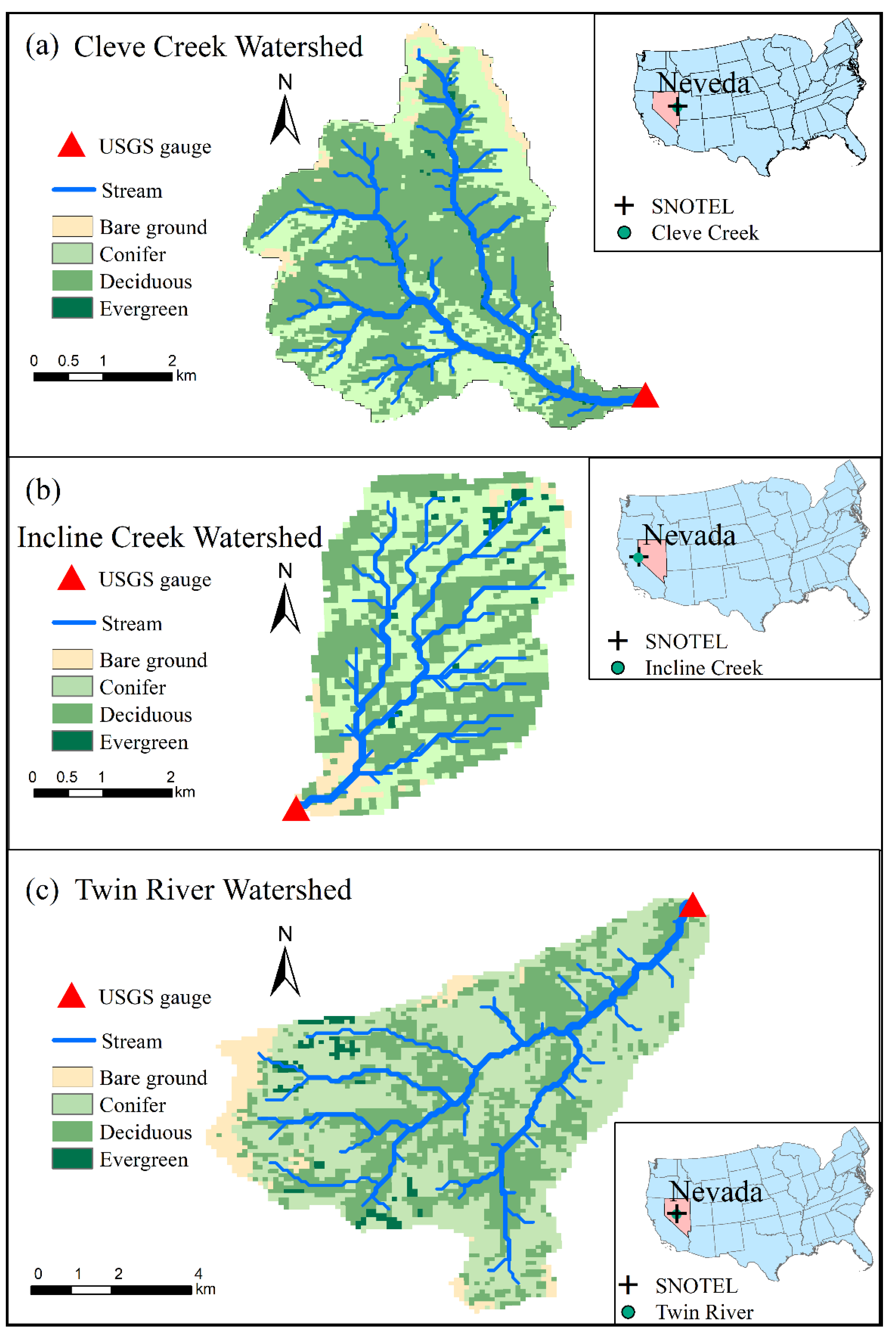
Three mountain watersheds (Cleve Creek (Figure 1a), Incline Creek (Figure 1b) and Twin River (Figure 1c)) located in Nevada, U.S., are investigated for the following reasons: (1) these mountain watersheds have warm summers and cold winters with annual mean temperatures ranging from 1.9 to 7.1 °C [35]; (2) the annual mean temperature of these watersheds have an overall increasing trend in recent years [10,36] as shown in Figure 2. The annual mean temperature approximately increases 1.5 °C in Cleve Creek watershed and Incline Creek watershed, individually. At Twin River watershed, the annual mean daily temperature increases around 4 °C; (3) long-term historical streamflow observations recorded by the US Geological Survey gauge stations can be employed to calibrate and evaluate model simulations; (4) these watersheds covered by multiple types of vegetation such as evergreen, deciduous, shrub and grass are suitable for investigating the connections between ecological and hydrological processes.
2.2. Weather Forcing Data
By incorporating the module of estimating the daily GSI to the updated CHESS model, the time series of daily maximum and minimum temperature (°C), as well as total precipitation (mm) are required as inputs. The daily weather records from the nearest SNOwpack TELemetry (SNOTEL) stations are employed to derive the weather forcing data since there is no weather station located in these watersheds. Because elevation differences exist between the SNOTEL station and the corresponding watershed, we apply the local lapse rate for adjusting the effect of elevation on daily maximum temperature, daily minimum temperature and daily total precipitation, individually. Table 1 shows the parameters we used in this study.
The separation of precipitation into snow and rainfall is necessary for a water balance calculation in a cold region. The separation step is essential to determine whether water is available for runoff and soil infiltration, or stored as snow. The snow proportion is a function of daily minimum and maximum threshold temperatures. If the average temperature is greater than the maximum threshold temperature, then all precipitation is considered as rainfall. If the average temperature is smaller than the minimum threshold temperature, then the precipitation is considered to fall as snow. When the average temperature is between the minimum and maximum threshold temperature, the rainfall proportion of the mixed precipitation is calculated by dividing the difference between the maximum threshold and average temperature by the difference between the minimum and maximum threshold temperatures. The other portion of the precipitation is considered as snow. The equation is presented as,
where Pr represents the portion of rainfall. TAve is the daily average temperature. TTMin and TTMax is the minimum and maximum threshold temperature in degree Celsius, respectively. For all tests, TTMin = −0.1 °C and TTMax = 0.1 °C [36].
2.3. Estimating Start of Growing Season (SOS)
There are numerous studies to investigate phenology shift such as species-level observations, satellite remote sensing of ecosystem production and atmospheric monitoring of carbon dioxide concentrations [37,38,39]. Previous studies have shown that minimum temperature, vapor pressure deficit (VPD) and photoperiod are the common set of meteorological variables leading to the variation in the seasonal phenology [40,41]. The product of these three indicators develops a combined model of the GSI that is calculated daily and integrated as a 21-day running average to avoid reaction to short-term changes in environmental conditions [42].
Minimum temperature: Many of the biochemical processes of plants are sensitive to low temperatures [43]. Although ambient air temperatures certainly have an impact on plant growth, constraints on phenology are more closely related to restrictions on water uptake by roots when soil temperatures are suboptimal [44]. The minimum temperature is a strong indicator for predicting the onset of plant growth. To incorporate a range of species, we choose a range encompassed by a lower minimum temperature threshold of −2 °C (TMMin) and an upper threshold of 5 °C (TMMax) [43]. To eliminate the effect of the unit, the minimum temperature index (iTmin) is presented as follows [42]:
where iTMin is the daily indicator for minimum temperature and is bounded between 0 and 1 and TMin is the observed daily minimum temperature in degrees Celsius. For all tests, TMMin = −2 °C and TMMax = 5 °C [42].
Vapor pressure deficit (VPD): water stress causes partial to complete stomatal closure, reduces leaf development rate, induces the shedding of leaves and slows or halts cell division. Since it is complicated to describe all the processes, the VPD of the atmosphere is selected as an index of the evaporative demand as a surrogate in this study. At low values, latent heat losses are not going to exceed available water. At high values, photosynthesis and growth are significantly restricted. Previous studies recommend that VPD less than 900 Pa should exert little effect on stomata whereas values greater than 4100 Pa generally are sufficient to force complete stomatal closure, even when the soils are moist [45,46]. Although these restrictions are various by locations and species, we select a widely used set of parameters (VPDMin = 900 Pa and VPDMax = 4100 Pa) in this research [41]. The VPD index (iVPD) is provided as follows:
where iVPD is the daily indicator for VPD and is bounded between 0 and 1 and VPD is the observed daily VPD in Pascals. For all tests, VPDMin = 900 Pa and VPDMax = 4100 Pa.
Photoperiod: photoperiod is a credible annual climatic cue for plants because it can be kept within a small range in different years at a given location. Studies have shown that photoperiod is critical for both leaf flush and leaf senescence throughout the world [47]. The photoperiod index (iPhoto) is given as follows:
where iPhoto is the daily photoperiod indicator and Photo is the daily photoperiod in seconds. For all tests, PhotoMin = 36,000 s (10 h) and PhotoMax = 39,600 s (11 h) [41].
GSI is a daily indicator of the relative constraints to foliar canopy development or maintenance due to climatic limits. The product of the three indices quantifies the GSI that is calculated daily and integrated as a 21-day running average to avoid reaction to short-term changes in environmental conditions [42]. The daily metric iGSI is presented as follows:
where iGSI is the daily GSI, iTmin, iVPD and iPhoto are the minimum temperature indicator, the VPD indicator and the photoperiod indicator, respectively. The daily GSI is then calculated as the 21-day moving average of the daily indicator, iGSI. The moving average serves to avoid single extreme events from prematurely triggering canopy changes.
The iGSI values are computed daily at each watershed using the parameters in Equations (2)–(5). The satellite-derived NDVI is used for validating the mean iGSI for the corresponding 8-day satellite data composite period. Phenology observations are averaged over all species for each observation date. The average date of leaf flushing is defined when the average canopy leaf area exceeds 10% of the seasonal maximum. Conversely, the average date of leaf coloration is defined as the date when leaf coloration exceeded 90%. The SOS is defined as the time when iGSI exceeds 0.5 in the spring and the EOS (end of growing season) is defined as the time when iGSI drops to 0.5 in the fall [41].
To find the impact of SOS on streamflow, the influences caused by temperature increase should be isolated. Two cases with the application of the updated CHESS model in these three watersheds are proposed. In each case, two scenarios at different temperatures are performed. One scenario is under the normal temperature condition. The other scenario is simulated under the condition that the temperature is 2 °C higher than the normal temperature throughout the whole year. The simulation is performed in the entire period from 1981 to 2017. Since the precipitation is abundant and the difference between the normal temperature and high temperature scenario is obvious for the three watersheds in 1995, we select the year 1995 to illustrate the specific variations of soil water storage (SWS), evaporation, transpiration, and streamflow when the temperature increases. The first case simulates the evaporation, SWS, and streamflow without vegetation in 1995 and is used as a baseline. Because the plant is removed in this case, the transpiration is 0 in this simulation. The second case is used for investigating the impact of varying SOS on evaporation, SWS, and streamflow with vegetation in 1995. The other conditions are the same as the previous case.
3. Results
3.1. Model Validation
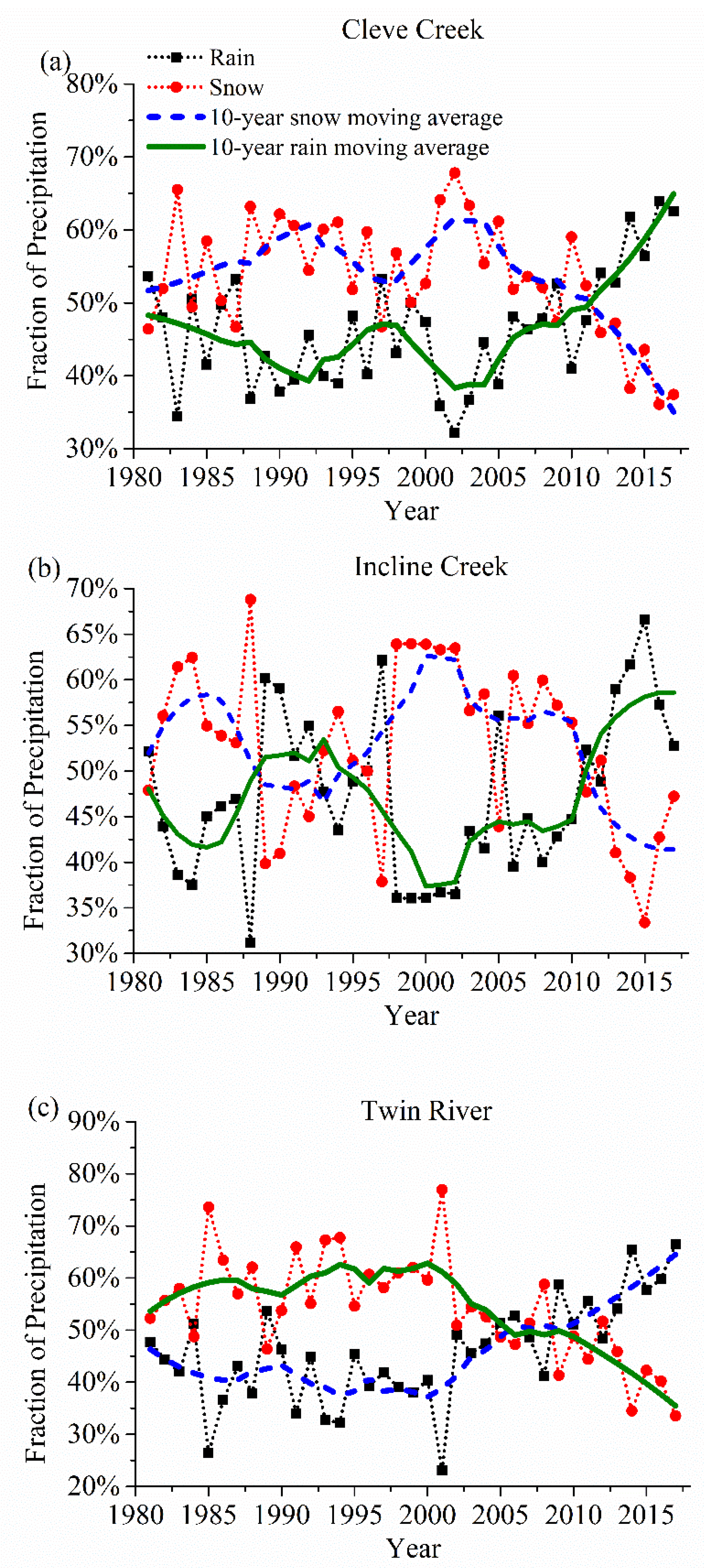
Figure 3 shows the percentage of snow in precipitation in the recent 37 years. To reduce the high-frequency variability, we applied a 10-year moving average to remove statistical uncertainties and smooth the annual value of each phenological event. Although snow occupies the main fraction in several years such as 2001–2003 in these three watersheds, a shift from snow towards rainfall becomes the dominating trend related to the potential global warming. The percentage of snow in Cleve Creek, Incline Creek and Twin River watersheds decreases by more than 5%, 10%, and 12% as the annual temperature rises around 1.5 °C, 1.5 °C and 4.0 °C, respectively.
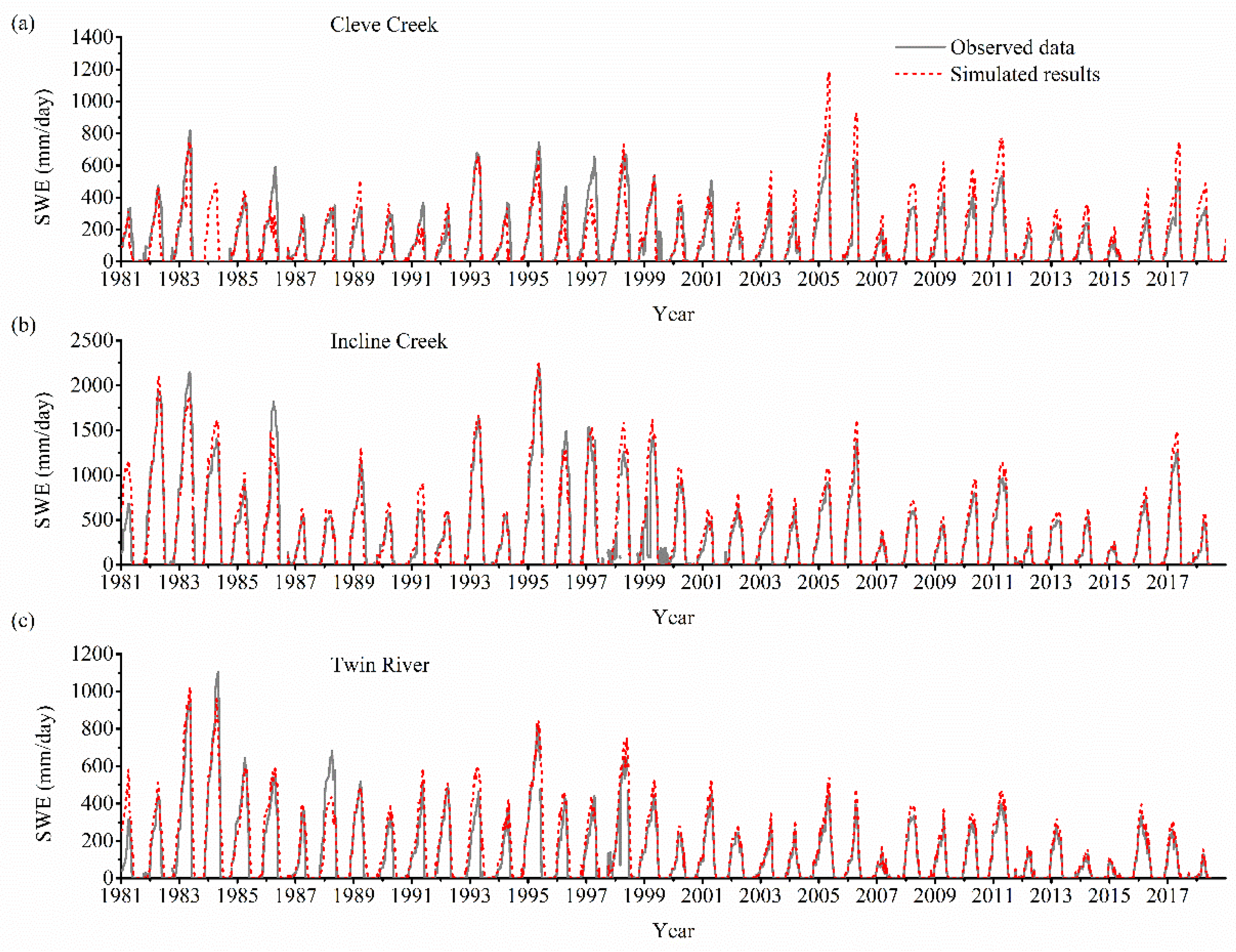
The calculated SWE from 1981 to 2017 are validated with the observed data in Figure 4. We notice that the updated CHESS model can simulate the variation of SWE in the three watersheds well. However, there are still several discrepancies between the simulated results and the observed data at the peaks (e.g., Cleve Creek watersheds in 2005, Incline Creek watersheds in 1991 and Twin River watersheds in 1993). The discrepancies may be caused by the spatial and temporal variation in the physical characteristics of the snow pack (e.g., the snow density, structures, and snow grain size) [48]. The algorithm may overestimate or underestimate the parameter in the updated CHESS model based on the hypothesis that the snow grain size is uniform both temporally and spatially.
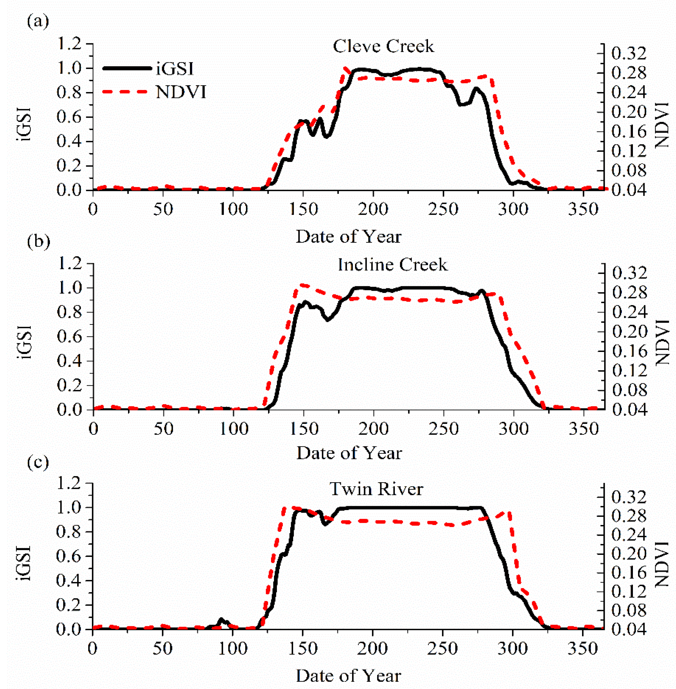
Time-series plots of iGSI and NDVI values for these three watersheds are also calculated from 1981 to 2017. Since the results of every year in this period are similar, we only choose one year (2001) to display as an example in Figure 5. The NDVI obtained from MODerate-resolution Imaging Spectroradiometer (MODIS) are used for validating the calculated iGSI. The image of NDVI contains 16 days of data, with the image’s data occurring on the 9th day of the 16-day period. This product combines the data choosing the best representative pixel from the 16-day period [49]. In Figure 5, the iGSI-predicted dynamics of growing season for the three watersheds agree with the observed NDVI well especially the start date and the end date. In these three cases, the updated CHESS model can accurately predict a rise at around the 130th day and a drop at around the 300th day. In other words, the updated CHESS model can precisely find SOS and EOS in a year. However, obvious difference can be observed within the growing season. This is because the updated CHESS uses the average parameter to calculate the iGSI for the diversity of plants.
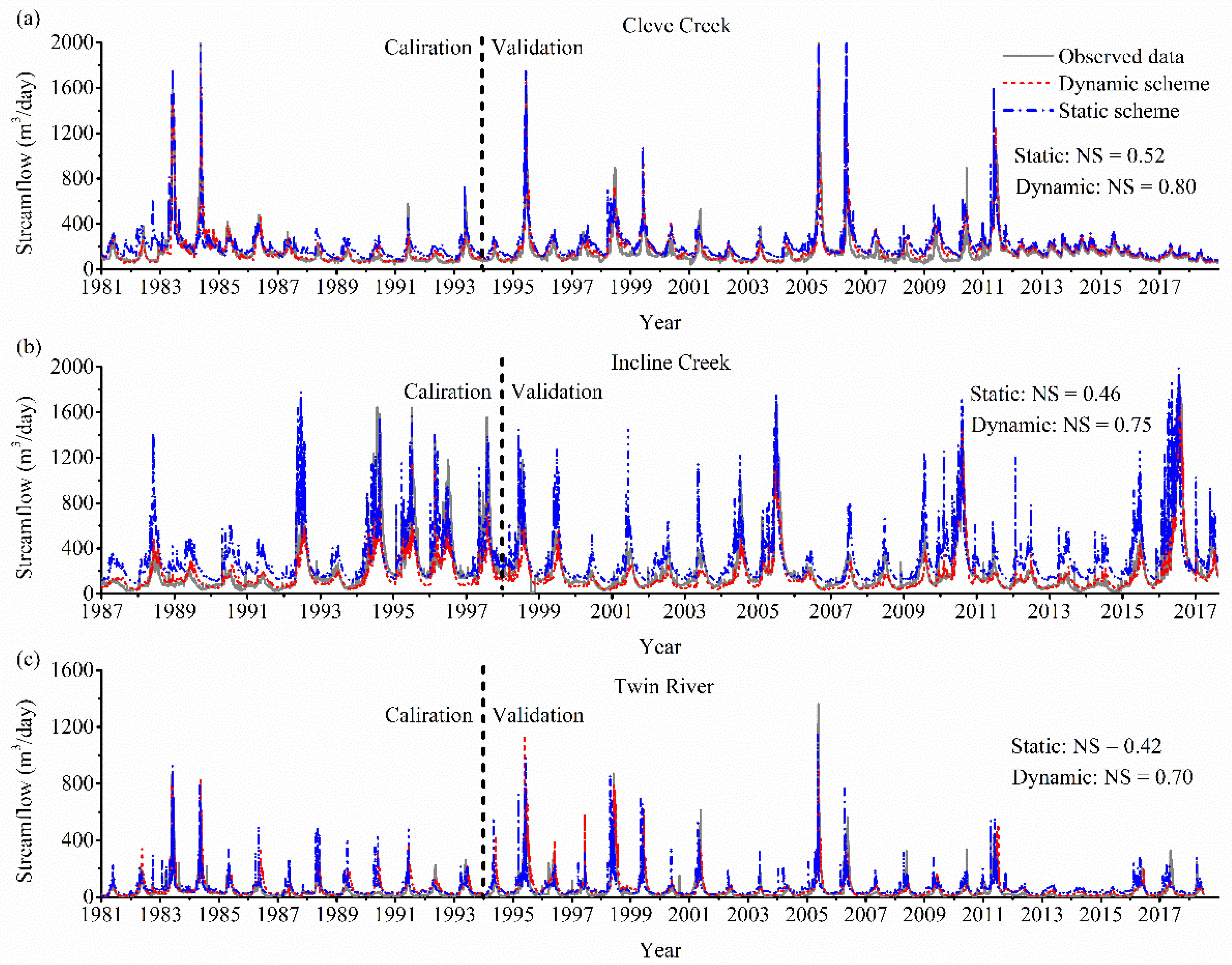
Figure 6 describes the comparison between the observed and the simulated streamflow under the dynamic and static scheme in the three watersheds. The static phenology scheme approximately captures the observed data with the NS (Nash–Sutcliffe model efficiency coefficient) in the study period (Cleve Creek: NS = 0.52; Incline Creek: NS = 0.46; Twin River: NS = 0.42). The dynamic phenology scheme improves the simulation (Cleve Creek: NS = 0.80; Incline Creek: NS = 0.75; Twin River: NS = 0.70). The main reason for improving the calculation in the dynamic scenario is that the ET has dramatic variations for all these three watersheds when full vegetation dynamics are incorporated. The updated CHESS model precisely estimates the ET as the growing season becomes longer. The annual streamflow calculated in the dynamic scheme is always smaller than that in the static scheme. Compared to the static scheme (Cleve Creek: RMSE = 0.02–0.26 m3/day; Incline Creek: RMSE = 0.02–0.18 m3/day; Twin River: RMSE = 0.04–0.22 m3/day), the CHESS model under the dynamic scheme improve the calculating accuracy (Cleve Creek: RMSE = 0.01–0.13 m3/day; Incline Creek: RMSE = 0.01–0.15 m3/day; Twin River: RMSE = 0.02–0.19 m3/day). Additionally, the peak of streamflow simulated in the dynamic scenario is closer to the observed data than that in the static scenario. When the SOS becomes earlier and the EOS becomes later, the CHESS model under the dynamic scheme can consistently improve the calculating accuracy.
3.2. Changes in SOS and End of Growing Season (EOS)
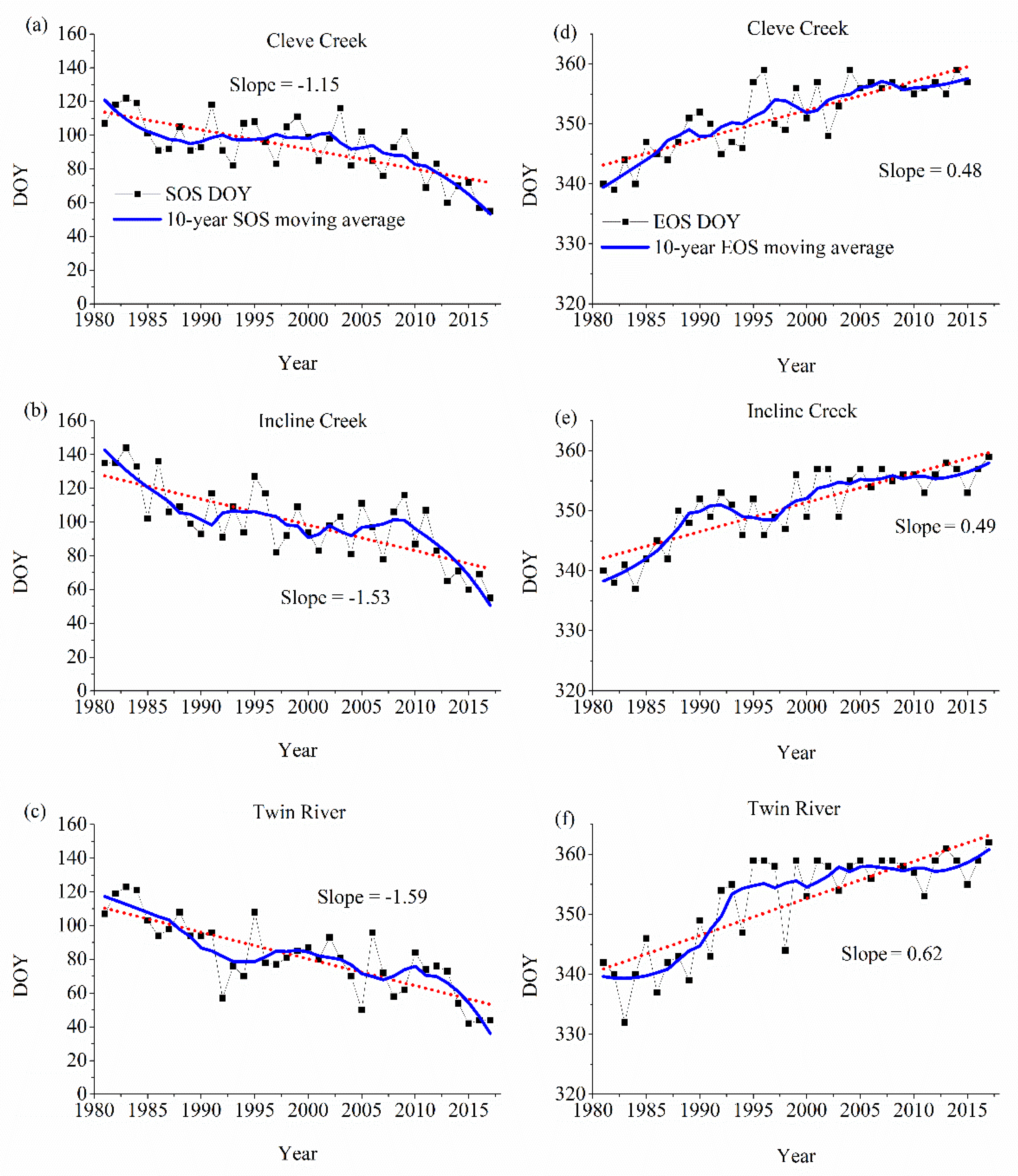
Figure 7 depicts the interannual variations of SOS and EOS from 1981 to 2017 in the three watersheds. As seen in Figure 7a–c, the climatological SOS dates are widely distributed from 70 days (approximately 20 March) to 120 days (approximately 1 May). In Cleve Creek watershed, the SOS is about 20 days earlier in 2017 than in 1981. The SOS of Incline Creek and Twin River watersheds is around 40 days earlier in 2017 than in 1981, respectively. Although several years show anomalies whereas the SOS of 1995 and 2006 are late in Twin River watershed, overall the timing of the onset displays earlier trends in the three watersheds. It shows that there is a high correlation between the temperature increase and the timing of the onset. The greater increase occurs to the watershed where the SOS comes earlier. The EOS dates in the three watersheds occur around the 340th day in December. They have the same spatial distributions that are opposite to SOS date (Figure 7d–f). The EOS becomes late as temperature increases, which illustrates the EOS also has a strong connection to the temperature increase that vegetation can last longer in a warmer climate. The watersheds with earlier SOS and later EOS show a longer growing season. The changes of the SOS and the EOS have high interannual variations. For example, significant changes in the SOS occur around 2000–2005, 1995–1998, 1992–1996 in Cleve Creek, Incline Creek and Twin River watershed, respectively. The dramatic variations of the EOS happen around 1995–1998, 1999–2003, and 1995–2000 in Cleve Creek, Incline Creek, and Twin River watershed, individually. To reduce the high-frequency variability, we applied a 10-year moving average to remove statistical uncertainties and smooth the annual value of each phenological event as shown in Figure 7. We note that the long-term variations in SOS display the earlier spring feature. In contrast to SOS, the long-term variations in EOS show the later autumn feature. Symmetric variation of SOS and EOS lead to an increase in the total length of the growing season. Linear trends of SOS during 1981–2017 are negative at −1.15, −1.53 and −1.59 day/year in Cleve Creek, Incline Creek and Twin River watershed, respectively. In contrast to SOS, Linear trends to EOS during 1981–2017 are positive at 0.48, 0.49 and 0.62 day/year.
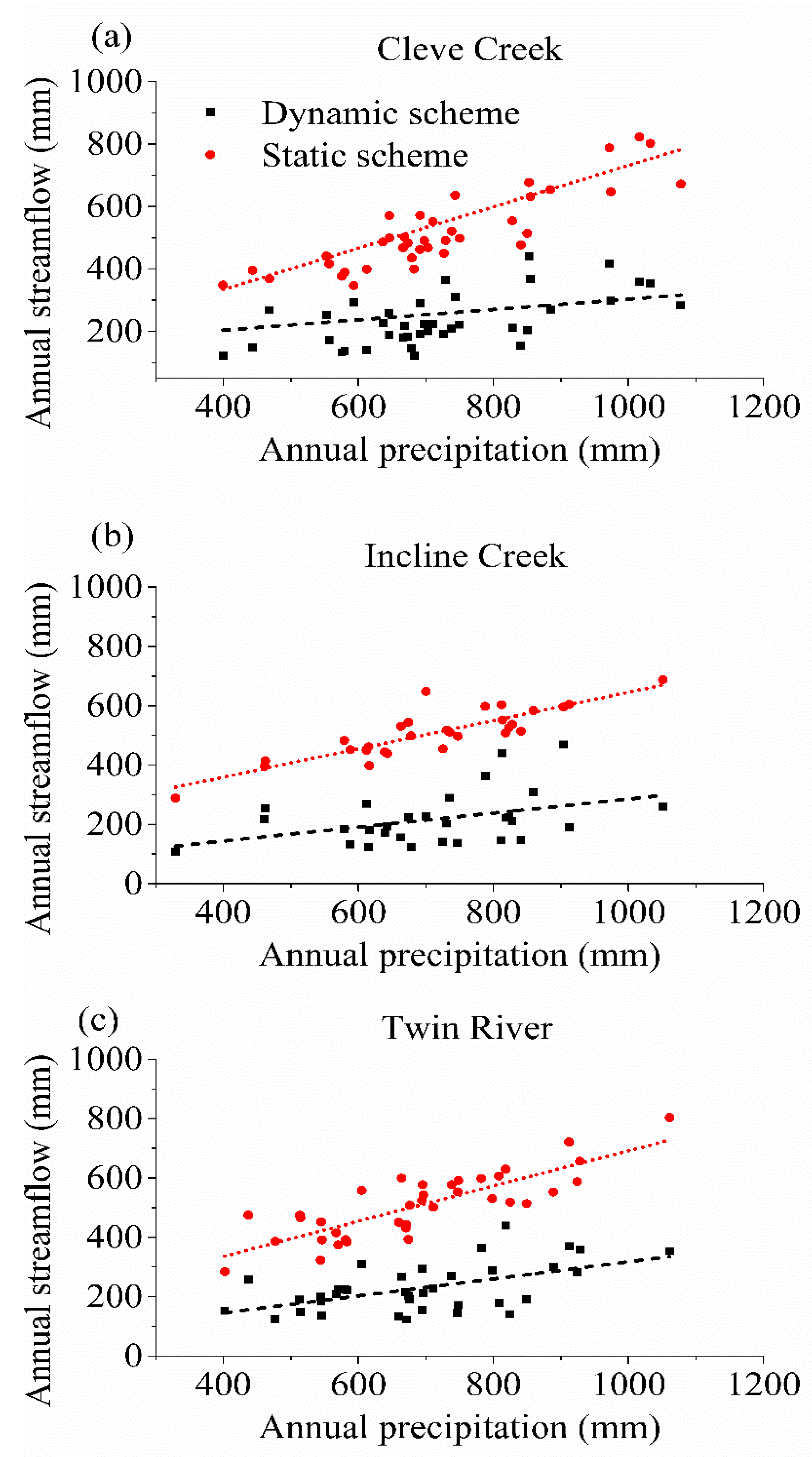
The interplay between precipitation and streamflow in the dynamic and static scheme is plotted in Figure 8. The relationship between the annual precipitation and streamflow is similar for the three watersheds. The increment speed of annual streamflow in the static scheme is faster than that in the dynamic scheme as the annual precipitation increases. The difference between the static and dynamic scheme is small in the low precipitation. The percentage of streamflow distributes within 70–87% and 31–38% in the static and dynamic scheme, respectively, while the percentage of the streamflow distributes within 62–76% and 25–33% in the high precipitation, individually. The results illustrate that the streamflow is overestimated in the static scheme because the static scheme underestimates the water consumption caused by the extended growing season. When the precipitation increases and provides sufficient water to the vegetation, the difference between these two schemes become large, which means the transpiration stands a larger proportion of precipitation.
3.3. The Impact of Varying SOS
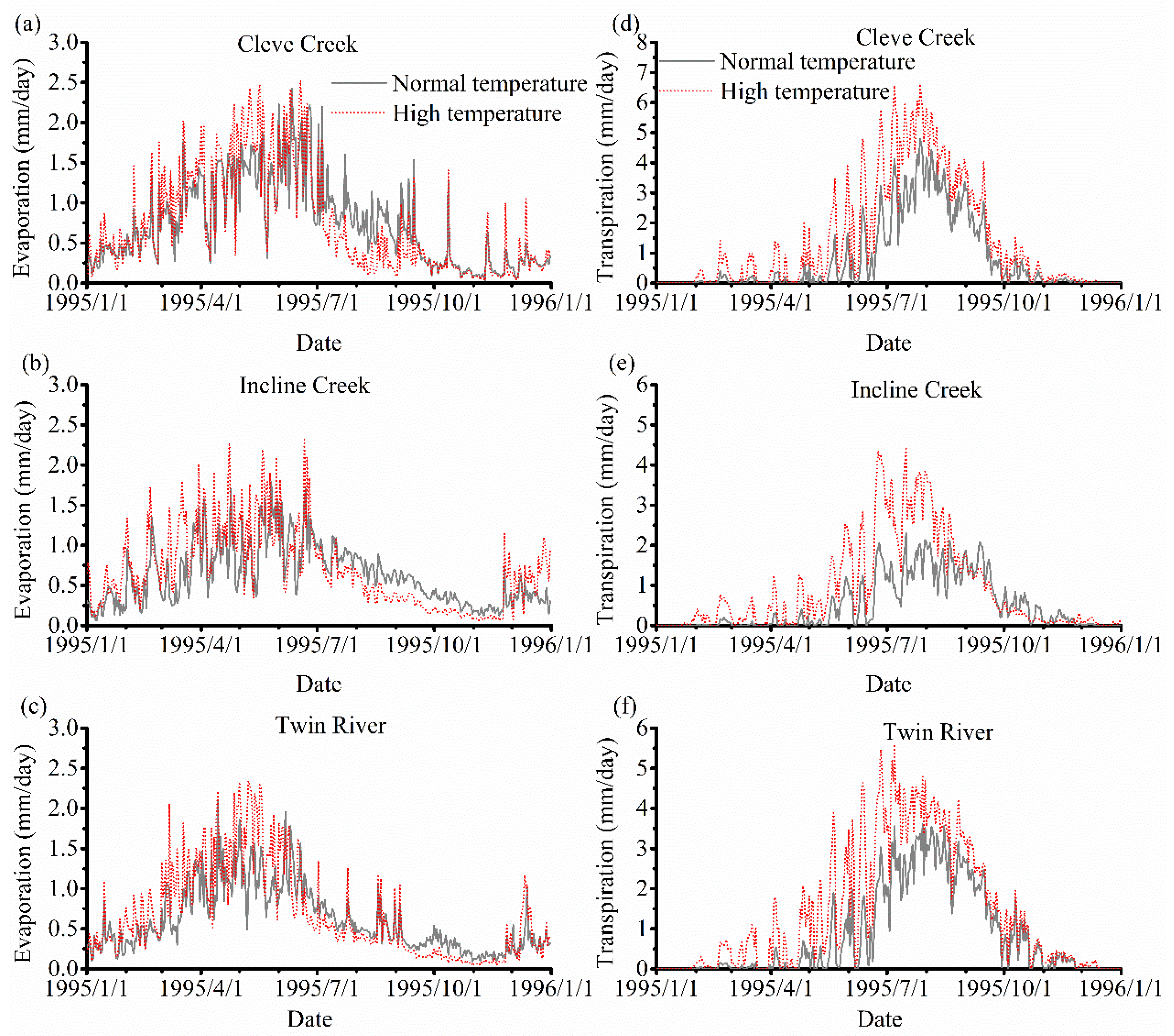
Figure 9 presents the influence of the temperature on the evaporation. When the temperature becomes higher, the evaporation increases more. Both scenarios have the maximum evaporations around July in the three watersheds. Most of the time, the evaporation in the high-temperature scenario is greater than the evaporation in the low-temperature scenario due to more snowmelt and rainfall occurring in the high-temperature scenario.
Figure 10a–c compares the SWS under these two scenarios. Most of the SWS in the high-temperature scenario before May is greater than that in the low-temperature scenario. This is due to higher infiltration caused by higher temperature. When precipitation in summer and autumn decreases, the soil storage, however, remains almost the same. The SWS has a significant increase in the high-temperature scenario after October 1st in the Incline Creek and Twin River watersheds because new snow falls.
The comparison of streamflow in these two scenarios is plotted in Figure 10d–f. In the Cleve Creek watershed, the variations of the stream flows are quite similar under these two scenarios where the maximum streamflow occurs in June. Because the evaporation and the soil storage are greater in the high-temperature scenario, the maximum streamflow in the high-temperature scenario is smaller than those in the low-temperature scenario. In the Incline Creek and Twin River watersheds, higher temperature causes the maximum streamflow occur much earlier. The streamflow in these two scenarios gradually converges after the snow melts.
Figure 11a–c plot the results of evaporation with vegetation under two different temperature scenarios. The evaporation in the high-temperature scenario is much greater than that in the low-temperature scenario before May but the difference between these two scenarios gradually decreases after May. On the other hand, there is a short period in the three watersheds when the evaporation in the low-temperature scenario is higher than that in the high-temperature. The main reason is that all the snow melts more quickly in the high-temperature scenario while a portion of the snow is still melting in the low-temperature scenario. We note that this period does not occur in the simulation without vegetation because the consumption of water from transpiration is much higher than the evaporation and the limited water is consumed at a faster rate in the vegetated simulation. If the SOS comes earlier, this period would last longer.
Figure 11d–f compares the transpiration in these two scenarios. The maximum transpiration occurs around July in the high-temperature scenario that is one month earlier than the normal temperature scenario. The transpiration is also much higher in the high-temperature scenario than that in the low-temperature scenario which shows the transpiration starts early and increases as the temperature increases. However, the difference of the transpiration between these two scenarios gradually decreases after July which means the EOS in various temperature does not significantly affect the transpiration.
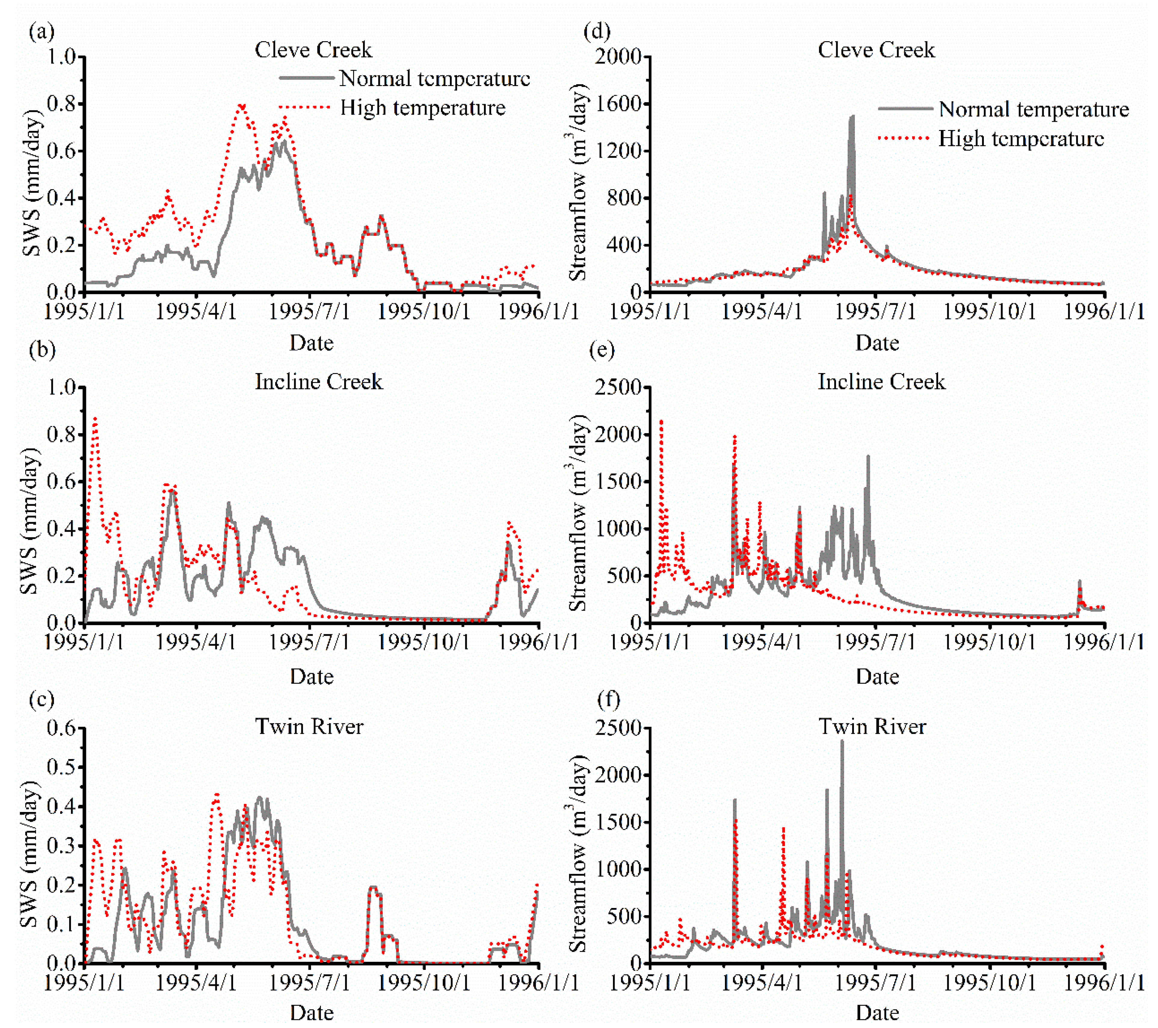
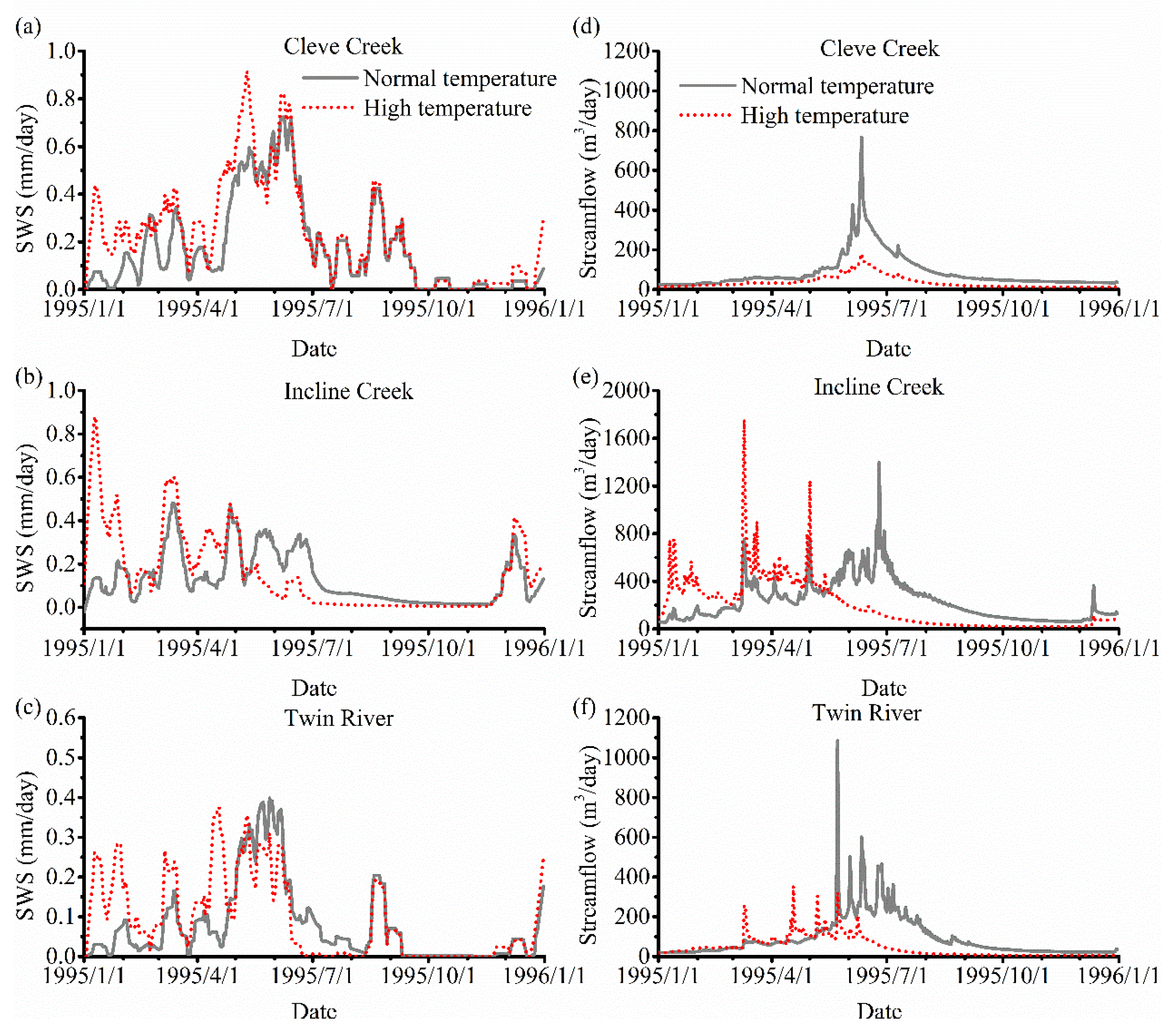
Figure 12a–c shows the results of SWS under these two temperature conditions. The SWS has a large variation before June and in general is greater in the high-temperature scenario than in the low-temperature scenario. We note that between May and October the SWS in the low-temperature scenario is greater than that in the high-temperature scenario in the Incline Creek and Twin River watershed because snow melting can last longer in the low-temperature scenario. When the precipitation occurs in November, the soil storage increases in the high-temperature scenario.
Figure 12d–f describes the streamflow under these two different temperature conditions. The streamflow in the low-temperature scenario is generally greater than that in the high temperature scenario in the Cleve Creek watershed. In the Incline Creek and Twin River watersheds, the streamflow in the high-temperature scenario is greater at the beginning of the year while the streamflow in the low-temperature scenario is greater after May. Compare to the streamflow without vegetation in Figure 10d–f, the streamflow under both various temperature scenarios with vegetation is smaller due to transpiration. As the temperature increases, the streamflow has an obvious increase because more snow melts and rainfall dominate the precipitation. However, the transpiration consumes a portion of the water which leads to the smaller streamflow. As the SOS becomes earlier, the peak of the stream with vegetation would come earlier.
4. Discussion
4.1. Drivers of the Vegetation Phenological Variations
The timing of SOS and EOS is controlled by different biological and environmental factors. In this study, we investigate several critical factors that have a great impact on vegetation phenology such as temperature, photoperiod and water availability. Temperature significantly affects vegetation phenology [50]. The temperature increase may lead to earlier spring and later autumn while temperature decrease may delay the timing of spring and advances of autumn [37]. A warming environment enhances the meristem cells to be stimulated and plant cell elongation to accelerate [51]. In this study, the annual temperature of the three watersheds approximately increases by 2 °C. Photoperiods also play a key role to control autumn phenological events such as leaf senescence [52]. The shortened photoperiod induces bud set and senescence when the photoperiod is smaller than the threshold of the growing-permitting period [53]. Water availability greatly affects plant Phenology in the vegetated watersheds [54]. Two impact factors, the timing of snow cover and snowmelt, notably alter plant phenology, particularly for shrubs and grasses at high altitudes and latitudes [55]. The varying snow effect also can alter the interaction between plant phenology, soil water content, and soil temperature. A portion of snow meltwater infiltrates into the frozen soil when the snow melts in early spring in a warming environment, which stimulates root activities even before the air temperature rises above zero and brings forward the timing of spring phenology [56].
4.2. The Effect of Vegetation Phenology on Evapotranspiration (ET) and Streamflow
We find that the ET values have increased greatly under the vegetation phenology scheme in the three vegetated watersheds. Transpiration plays the largest role in the total evapotranspiration during the growing season. This is consistent with the previous research that the percentage of transpiration, forest floor evaporation, and interception evaporation is 65%, 15%, and 20%, respectively [57]. The reason for the increase of ET is mainly attributed to the extended growing season lengths. Within the extended growing season, soil evaporation is in the opposite direction to transpiration and canopy evaporation due to the canopy interception which results in reducing soil water and soil evaporation.
Previous studies have demonstrated that climate warming is the main driver for streamflow decrease [58,59]. Consistent with these studies, both SOS and EOS are strongly linked with streamflow. Vegetation growth in the long-term plays a more vital role. When the SOS comes earlier and EOS terminates later, extra water consumed by vegetation may result in an aggravating decrease of soil water and groundwater. Therefore, water discharge in streams tends to decrease because precipitation would firstly supply soil deficit and recharge groundwater. The earlier SOS and delayed EOS accelerate the process of water transfer from land surface to the atmosphere dramatically because transpiration is the largest proportion of evapotranspiration [60,61].
We note that the vegetation phenology dynamics significantly affect the streamflow of these three watersheds during the last three decades and interact with long-term increase and interannual variability in growing season length. In this study, the streamflow decreases the dynamic ecosystem response to varying climate being integrated, which is consistent with the result that the increase of growing season lengths is attributed to daily minimum temperatures in spring and autumn [62]. This illustrates that the extended growing season increases vegetation water use and leaf interception in the watersheds. Vegetation first intercepts the precipitation and infiltrated water is mainly consumed via transpiration [63,64], which results in the decrease of water discharge to the stream.
4.3. Long-Term Influence of Early SOS
The extension of the growing season has been associated with recent global warming. Changes in the SOS not only have far-reaching consequences for plant and animal ecosystems but also may lead to long-term decreases in streamflow and changes in vegetation cover which affect the climate system. If the shifts in SOS observed in this study continue, they have critical implications for reservoir operations. Snowmelt occurs earlier, and the growing season may increase in length caused by earlier SOS, which may reduce the risk of flooding during snowmelt. On the other hand, flood risk might increase if the temperature persistently increases. Earlier SOS may cause soil moisture to decline during summer, increasing drought stress in trees, leading to high risk of wildfires and insect infestation.
Land surface roughness refers to the configuration or microrelief. Flow resistance determines the speed with which surface runoff responds. By affecting the time by which surface runoff remains on the land surface, the roughness also influences the volume of water that can infiltrate into the soil. In many parts of the northern hemisphere, studies indicated that the onset of growing season comes at least a week to 10 days earlier over the 20th century [65]. If this pattern of early SOS continues, as expected in response to continued climate warming, the effects on annual rates of transpiration could be significant. Increases in early spring transpiration would likely result in earlier declines in soil moisture content, declines in summer seasonal streamflow, lower summer base flow, and longer periods of summer low flow conditions. Watersheds are strongly correlated with total runoff because vegetated soil has greater roughness and higher capacity for infiltration [66]. The magnitude of the peak for the streamflow will become smaller and earlier, leading to flattened hydrographs.
4.4. Future Work
This study presents the drivers, mechanisms and the hydro-ecological response to the warming climate. However, several challenges need to be improved in future studies. The current model employs empirical parameters via a statistical relationship to describe plant growth. Lacking vegetational mechanisms may cause uncertainties when predicting phenology feedback in future climate. Inverse modeling methods can help to reduce the uncertainties by incorporating eco-physiological and morphological responses [56]. More climate manipulation experiments are needed to investigate the processes controlling plant phenological dynamics and to improve the CHESS model. Root production contributes to 33–67% of the terrestrial net primary production [67], and the response of root phenology to climate change is quite different from the aboveground phenology [68]. Maintaining species coexistence in multispecies plant communities is essential in plant phenology. Ongoing climate change alters the timing and length of phenological events, which may desynchronize seasonal interactions among species, resulting in altered biodiversity and ecosystem primary productivity [69]. Our model has the limitation that the species of the vegetation are constant in varying climate conditions. Filling such knowledge gaps can help us to better understand and predict plant phenological variations in response to the ongoing climate change.
5. Conclusions
The simulated results show that the updated CHESS model can accurately predict the variation of SWE in the three watersheds. But discrepancies between the simulated results and the observed data occur at the peaks due to the spatial and temporal variation in the physical characteristics of the snowpack. The static algorithm may overestimate or underestimate the parameters in the updated CHESS model based on the hypothesis that the snow grain size is uniform both temporally and spatially. By incorporating the GSI module, the updated CHESS model can be used to examine the timing of SOS and EOS. The simulated iGSI has been validated by NDVI from MODIS containing 16 days of data. The results indicate there is a high relationship between the temperature and the timing of the SOS and EOS. The SOS starts earlier and EOS ends later in a year when the watershed has a greater temperature increase. The streamflow in the static and dynamic scheme in the three watersheds are simulated between 1981 and 2017 with the NS of 0.52 and 0.80 in Cleve Creek, 0.46 and 0.75 in Incline Creek, and 0.42 and 0.70 in the Twin River watersheds, respectively.
Compared to the streamflow without vegetation, the streamflow under the two temperature scenarios with vegetation is smaller. As the temperature increases, the streamflow has an obvious increase with more snow melts and more rainfall-dominated precipitation. However, the transpiration leads to flattened streamflow hydrographs. As the SOS becomes earlier, the peak of the stream with vegetation occurs earlier. If the shifts in SOS observed in this study continue, the effects on annual rates of transpiration could be large and the growing season may increase in length, which may reduce the risk of flooding during snowmelt. On the other hand, flood risk may increase if temperature persistently increases.
Author Contributions
Calculation, conceptualization, visualization and writing, funding acquisition, H.F.; review and editing, J.Z.; formula analysis and model validation, visualization, M.S.; data collection and investigation, X.C. All authors have read and agreed to the published version of the manuscript.
Funding
This research was funded by the Sun Yat-sen University’s Basic Research Fund for Young Scholars (No. 201gpy30).
Institutional Review Board Statement
Not applicable.
Informed Consent Statement
Not applicable.
Data Availability Statement
The data displayed in this study is available in the current manuscript.
Acknowledgments
We highly appreciate the valuable comments from anonymous reviewers that greatly improved our manuscript.
Conflicts of Interest
The authors declare no conflict of interest.
References
- Enzminger, T.L.; Small, E.E.; Borsa, A.A. Accuracy of Snow Water Equivalent Estimated From GPS Vertical Displacements: A Synthetic Loading Case Study for Western U.S. Mountains. Water Resour. Res. 2018, 54, 581–599. [Google Scholar] [CrossRef]
- Serreze, M.C.; Clark, M.P.; Armstrong, R.L.; McGinnis, D.A.; Pulwarty, R.S. Characteristics of the western United States snowpack from snowpack telemetry (SNOTEL) data. Water Resour. Res. 1999, 35, 2145–2160. [Google Scholar] [CrossRef] [Green Version]
- Tamaddun, K.A.; Kalra, A.; Bernardez, M.; Ahmad, S. Multi-Scale Correlation between the Western U.S. Snow Water Equivalent and ENSO/PDO Using Wavelet Analyses. Water Resour. Manag. 2017, 31, 2745–2759. [Google Scholar] [CrossRef]
- Dierauer, J.R.; Allen, D.M.; Whitfield, P.H. Snow drought risk and susceptibility in the western United States and southwestern Canada. Water Resour. Res. 2019, 55, 3076–3091. [Google Scholar] [CrossRef]
- Lapo, K.E.; Hinkelman, L.M.; Raleigh, M.S.; Lundquist, J.D. Impact of errors in the downwelling irradiances on simulations of snow water equivalent, snow surface temperature, and the snow energy balance. Water Resour. Res. 2015, 51, 1649–1670. [Google Scholar] [CrossRef]
- Gergel, D.R.; Nijssen, B.; Abatzoglou, J.T.; Lettenmaier, D.P.; Stumbaugh, M.R. Effects of climate change on snowpack and fire potential in the western USA. Clim. Chang. 2017, 141, 287–299. [Google Scholar] [CrossRef]
- Kelleners, T.J.; Chandler, D.G.; McNamara, J.P.; Gribb, M.M.; Seyfried, M.S. Modeling runoff generation in a small snow-dominated mountainous catchment. Vadose Zone J. 2010, 9, 517–527. [Google Scholar] [CrossRef] [Green Version]
- Papalexiou, S.M.; Montanari, A. Global and Regional Increase of Precipitation Extremes under Global Warming. Water Resour. Res. 2019, 55, 4901–4914. [Google Scholar] [CrossRef]
- Tague, C.; Grant, G.E. Groundwater dynamics mediate low-flow response to global warming in snow-dominated alpine regions. Water Resour. Res. 2009, 45. [Google Scholar] [CrossRef]
- Tang, G.; Arnone, J.A., III; Verburg, P.S.J.; Jasoni, R.L.; Sun, L. Trend and climatic sensitivity of vegetation phenology in semiarid and arid ecosystems in the US Great Basin during 1982–2011. Biogeosciences 2009, 12. [Google Scholar] [CrossRef] [Green Version]
- Vincent, L.A.; Zhang, X.; Hogg, W.D. Maximum and minimum temperature trends in Canada for 1895–1995 and 1945–1995. In Proceedings of the 10th Symposium on Global Change Studies, Dallas, TX, USA, 10–15 January 1999; pp. 95–98. [Google Scholar]
- Nayak, A.; Marks, D.; Chandler, D.G.; Seyfried, M. Long-term snow, climate, and streamflow trends at the Reynolds Creek Experimental Watershed, Owyhee Mountains, Idaho, United States. Water Resour. Res. 2010, 46, W06519.1–W06529.15. [Google Scholar] [CrossRef]
- Bonan, G.B. Forests and climate change: Forcings 2010, feedbacks, and the climate benefits of forests. Science 2008, 320, 1444–1449. [Google Scholar] [CrossRef] [PubMed] [Green Version]
- Hao, L.; Sun, G.; Liu, Y.; Zhou, G.; Wan, J.; Zhang, L.; Niu, J.; Sang, Y.; He, J. Evapotranspiration and soil moisture dynamics in a temperate grassland ecosystem in Inner Mongolia, China. Trans. ASABE 2016, 59, 577–590. [Google Scholar] [CrossRef]
- Sun, G.; Caldwell, P.; Noormets, A.; McNulty, S.G.; Cohen, E.; Moore, M.; Jennifer, D.; Treasure, E.; Mu, Q.; Xiao, J.; et al. Upscaling key ecosystem functions across the conterminous United States by a water-centric ecosystem model. J. Geophys. Res. 2011, 116, G00J05. [Google Scholar] [CrossRef]
- Hewlett, J.D.; Fortson, J.C.; Cunningham, G.B. The effect of rainfall intensity on storm flow and peak discharge from forest land. Water Resour. Res. 1977, 13, 259–266. [Google Scholar] [CrossRef]
- Sun, G.; Hallema, D.; Asbjornsen, H. Ecohydrological processes and ecosystem services in the Anthropocene: A review. Ecol. Process. 2017, 6, 1–9. [Google Scholar] [CrossRef] [Green Version]
- Andréassian, V. Waters and forests: From historical controversy to scientific debate. J. Hydrol. 2004, 291, 1–27. [Google Scholar] [CrossRef]
- Bruijnzeel, L.A. Hydrological functions of tropical forests: Not seeing the soil for the trees? Agric. Ecosyst. Environ. 2004, 104, 185–228. [Google Scholar] [CrossRef]
- Jackson, R.B. Trading water for carbon with biological sequestration. Science 2005, 310, 1944–1947. [Google Scholar] [CrossRef] [Green Version]
- Sun, G.; Riekerk, H.; Kornhak, L.V. Ground-water-table rise after forest harvesting on cypress-pine flatwoods in Florida. Wetlands 2000, 20, 101–112. [Google Scholar] [CrossRef]
- Fu, Z.; Stoy, P.C.; Luo, Y.; Chen, J.; Sun, J.; Montagnani, L.; Wohlfahrt, G.; Rahman, A.F.; Rambal, S.; Bernhofer, C.; et al. Climate controls over the net carbon uptake period and amplitude of net ecosystem production in temperate and boreal ecosystems. Agric. For. Meteorol. 2017, 243, 9–18. [Google Scholar] [CrossRef] [Green Version]
- Hmimina, G.; Yu, R.; Billesbach, D.P.; Huemmrich, K.F.; Gamon, J.A. Changes in Arctic and Boreal Ecosystem Productivity in Response to Changes in Growing Season Length; AGU Fall Meeting Abstracts: New Orleans, LA, USA, 2017. [Google Scholar]
- Dunn, A.L.; Barford, C.C.; Wofsy, S.C.; Goulden, M.L.; Daube, B.C. A long-term record of carbon exchange in a boreal black spruce forest: Means 2017, responses to interannual variability, and decadal trends. Glob. Change Biol. 2007, 13, 577–590. [Google Scholar] [CrossRef] [Green Version]
- Winchell, T.; Molotch, N.P.; Barnard, D.M. Early Snowmelt Decreases Ablation Period Carbon Uptake in a High Elevation, Subalpine Forest; AGU Fall Meeting Abstracts: Niwot Ridge, CO, USA, 2015. [Google Scholar]
- Wohlfahrt, G.; Cremonese, E.; Hammerle, A.; Hortnagl, L.; Galvagno, M.; Gianelle, D.; Marcolla, B.; di Cella, U.M. Trade-offs between global warming and day length on the start of the carbon uptake period in seasonally cold ecosystems. Geophys. Res. Lett. 2013, 40, 6136–6142. [Google Scholar] [CrossRef]
- Saksa, P.C.; Conklin, M.H.; Battles, J.J.; Tague, C.L.; Bales, R.C. Forest thinning impacts on the water balance of Sierra Nevada mixed-conifer headwater basins. Water Resour. Res. 2017, 53, 5364–5381. [Google Scholar] [CrossRef] [Green Version]
- Son, K.; Tague, C. Hydrologic responses to climate warming for a snow-dominated watershed and a transient snow watershed in the California Sierra. Ecohydrology 2019, 12, e2053. [Google Scholar] [CrossRef] [Green Version]
- Bell, C.D.; Tague, C.L.; McMillan, S.K. Modeling Runoff and Nitrogen Loads From a Watershed at Different Levels of Impervious Surface Coverage and Connectivity to Storm Water Control Measures. Water Resour. Res. 2019, 55, 2690–2707. [Google Scholar] [CrossRef]
- Shin, H.; Park, M.; Lee, J.; Lim, H.; Kim, S.J. Evaluation of the effects of climate change on forest watershed hydroecology using the RHESSys model: Seolmacheon catchment. Paddy Water Environ. 2019, 17, 581–595. [Google Scholar] [CrossRef]
- Shields, C.; Tague, C. Ecohydrology in semiarid urban ecosystems: Modeling the relationship between connected impervious area and ecosystem productivity. Water Resour. Res. 2015, 51, 302–319. [Google Scholar] [CrossRef]
- Doten, C.O.; Bowling, L.C.; Lanini, J.S.; Maurer, E.P.; Lettenmaier, D.P. A spatially distributed model for the dynamic prediction of sediment erosion and transport in mountainous forested watersheds. Water Resour. Res. 2006, 42. [Google Scholar] [CrossRef]
- Tang, G.; Schneiderman, E.M.; Band, L.E.; Hwang, T.; Zion, M.S. Does consideration of water routing affect simulated water and carbon dynamics in terrestrial ecosystems? Hydrol. Earth Syst. Sci. Discuss. 2014, 18, 12537–12571. [Google Scholar] [CrossRef] [Green Version]
- Tang, G.; Carroll Rosemary, W.H.; Lutz, A.; Sun, L. Regulation of precipitation-associated vegetation dynamics on catchment water balance in a semiarid and arid mountainous watershed. Ecohydrology 2016, 9, 1248–1262. [Google Scholar] [CrossRef]
- Tang, G.; Li, S.; Yang, M.; Xu, Z.; Liu, Y.; Gu, H. Streamflow response to snow regime shift associated with climate variability in four mountain watersheds in the US Great Basin. J. Hydrol. 2019, 573, 255–266. [Google Scholar] [CrossRef]
- Tang, G.; Arnone, J.A., III. Trends in surface air temperature and temperature extremes in the Great Basin during the 20th century from ground-based observations. J. Geophys. Res. Atmos. 2013, 118, 3579–3589. [Google Scholar] [CrossRef]
- Menzel, A.; Sparks, T.H.; Estrella, N.; Koch, E.; Aasa, A.; Ahas, R.; Alm-Kübler, K.; Bissolli, P.; Braslavská, O.G.; Briede, A.; et al. European phonological response to climate change matches the warming pattern. Glob. Change Biol. 2006, 12, 1969–1976. [Google Scholar] [CrossRef]
- Prodon, R.; Geniez, P.; Cheylan, M.; Devers, F.; Besnard, A. A reversal of the shift towards earlier spring phenology in several Mediterranean reptiles and amphibians during the 1998–2013 warming slowdown. Glob. Change Biol. 2017, 23. [Google Scholar] [CrossRef]
- Sillett, T.S.; Holmes, R.T.; Sherry, T.W. Impacts of a Global Climate Cycle on Population Dynamics of a Migratory Songbird. Science 2000, 288, 2040–2042. [Google Scholar] [CrossRef] [Green Version]
- Fu, Y.; Piao, S.; Delpierre, N.; Hao, F.; Hanninen, H.; Liu, Y.; Sun, W.; Janssens, I.A.; Campioli, M. Larger temperature response of autumn leaf senescence than spring leaf-out phenology. Glob. Change Biol. 2017, 24, 2159–2168. [Google Scholar] [CrossRef] [PubMed]
- Jolly, W.N.; Nemani, R.; Running, S.W. A generalized, bioclimatic index to predict foliarphenology in response to climate. Glob. Change Biol. 2005, 11, 619–632. [Google Scholar] [CrossRef]
- Lieberman, D. Seasonality and phenology in a dry tropical forest in Ghana. J. Ecol. 1982, 70, 791–806. [Google Scholar] [CrossRef]
- Larcher, W.; Bauer, H. Ecological significance of resistance to low temperature. In Physiological Plant Ecology; Springer: Berlin/Heidelberg, Germany, 1981; Volume 12, pp. 403–437. [Google Scholar] [CrossRef]
- Waring, R.H. Forest plants of the eastern Siskiyous: Their environmental and vegetational distribution. Northwest Sci. 1969, 43, 1–17. [Google Scholar]
- Osonubi, O.; Davies, W. The influence of plant water stress on stomatal control of gas exchange at different levels of atmospheric humidity. Oecologia 1980, 46, 1–6. [Google Scholar] [CrossRef]
- Tenhunen, J.D.; Lange, O.L.; Jahner, D. The control by atmospheric factors and water stress of midday stomatal closure in Arbutus unedo growing in a natural macchia. Oecologia 1982, 55, 165–169. [Google Scholar] [CrossRef]
- Borchert, R.; Rivera, G. Photoperiodic control of seasonal development and dormancy in tropical stem-succulent trees. Tree Physiol. 2001, 21, 213–221. [Google Scholar] [CrossRef]
- Xu, B.; Chen, H.; Sun, S.; Gao, C. Large discrepancy between measured and remotely sensed snow water equivalent in the northern Europe and western Siberia during boreal winter. Theor. Appl. Climatol. 2019, 137, 133–140. [Google Scholar] [CrossRef]
- Miranda-Aragón, L. NDVI-rainfall relationship using hyper-temporal satellite data in a portion of North Central Mexico 2000-2010. Afr. J. Agric. Res. 2012, 7, 1023–1033. [Google Scholar] [CrossRef]
- Chuine, I. Why does phenology drive species distribution? Philos. Trans. R. Soc. Lond. B Biol. Sci. 2010, 365, 3149–3160. [Google Scholar] [CrossRef] [PubMed] [Green Version]
- Hanninen, H. Boreal and Temperate Trees in a Changing Climate; Spirnger: Dordrecht, The Netherlands, 2016; Volume 3. [Google Scholar] [CrossRef]
- Cooke, J.E.; Eriksson, M.E.; Junttila, O. The dynamic nature of bud dormancy in trees: Environmental control and molecular mechanisms. Plant Cell Environ. 2012, 35, 1707–1728. [Google Scholar] [CrossRef] [PubMed]
- Wareing, P. Photoperiodism in woody plants. Annu. Rev. Plant Physiol. 1956, 7, 191–214. [Google Scholar] [CrossRef]
- Jaworski, T.; Hilszczański, J. The effect of temperature and humidity changes on insects development their impact on forest ecosystems in the expected climate change. For. Res. Pap. 2013, 74, 345–355. [Google Scholar] [CrossRef]
- Zeng, H.; Jia, G. Impacts of snow cover on vegetation phenology in the arctic from satellite data. Adv. Atmos. Sci. 2013, 30, 1421–1432. [Google Scholar] [CrossRef]
- Piao, S.; Liu, Q.; Chen, A.; Janssens, I.A.; Fu, Y.; Dai, J.; Liu, L.; Lian, X.; Shen, M.; Zhu, X. Plant phenology and global climate change: Current progresses and challenges. Glob. Change Biol. 2019, 25, 1922–1940. [Google Scholar] [CrossRef]
- Grelle, A.; Lundberg, A.; Lindroth, A.; Moren, A.S.; Cienciala, E. Evaporation components of a boreal forest: Variations during the growing season. J. Hydrol. 1997, 197, 70–87. [Google Scholar] [CrossRef]
- Tapash, D.; Pierce, D.W.; Cayan, R.D.; Vano, J.A.; Lettenmaier, D.P. The importance of warm season warming to western U.S. streamflow changes. Geophys. Res. Lett. 2011, 38, L23403. [Google Scholar] [CrossRef] [Green Version]
- Sun, Y.; Tian, F.; Yang, L.; Hu, H. Exploring the spatial variability of contributions from climate variation and change in catchment properties to streamflow decrease in a mesoscale basin by three different methods. J. Hydrol. 2014, 208, 170–180. [Google Scholar] [CrossRef]
- Yamazaki, T.; Yabuki, H.; Ishii, Y.; Ohata, T. Water and energy exchanges at forests and a grassland in eastern Siberia evaluated using a one-dimensional land surface model. J. Hydrometeorol. 2004, 5, 504–515. [Google Scholar] [CrossRef]
- Schlesinger, W.H.; Jasechko, S. Transpiration in the global water cycle. Agric. For. Meteorol. 2014, 189–190, 115–117. [Google Scholar] [CrossRef]
- Hwang, T.; Martin, K.L.; Vose, J.M.; Wear, D.; Miles, B.; Kim, Y.; Band, L.E. Nonstationary hydrologic behavior in forested watersheds is mediated by climate-induced changes in growing season length and subsequent vegetation growth. Water Resour. Res. 2018, 54, 5359–5375. [Google Scholar] [CrossRef]
- Brooks, J.R.; Barnard, H.R.; Coulombe, R.; McDonnell, J.J. Ecohydrologic separation of water between trees and streams in a Mediterranean climate. Nat. Geosci. 2010, 3, 100–104. [Google Scholar] [CrossRef]
- Wang, H.; Tetzlaff, D.; Buttle, J.; Carey, S.K.; Laudon, H.; McNamara, J.P.; Spence, C.; Soulsby, C. Climate-phenology-hydrology interactions in northern high latitudes: Assessing the value of remote sensing data in catchment ecohydrological studies. Sci. Total Environ. 2019, 656, 19–28. [Google Scholar] [CrossRef] [Green Version]
- Houghton, J.; Ding, Y.H.; Griggs, J.; Noguer, M.; Johnson, C.A. Physical climate processes and feedbacks 2001. In Climate Change 2001: The Scientific Basis; Cambridge University Press: Cambridge, UK, 2001; Chapter 7; pp. 419–470. [Google Scholar]
- Singh, V.P. Effect of spatial and temporal variability in rainfall and watershed characteristics on stream flow hydrograph. Hydrol. Process. 1997, 11, 1649–1669. [Google Scholar] [CrossRef]
- Abramoff, R.Z.; Finzi, A.C. Are above-and below-ground phenology in sync? New Phytol. 2015, 205, 1054–1061. [Google Scholar] [CrossRef] [PubMed]
- Steinaker, D.F.; Wilson, S.D.; Peltzer, D.A. Asynchronicity in root and shoot phenology in grasses and woody plants. Glob. Change Biol. 2010, 16, 2241–2251. [Google Scholar] [CrossRef]
- Kharouba, H.M.; Ehrlén, J.; Gelman, A.; Bolmgren, K.; Allen, J.M.; Travers, S.E.; Wolkovich, E.M. Global shifts in the phenological synchrony of species interactions over recent decades. Proc. Natl. Acad. Sci. USA 2018, 115, 5211–5216. [Google Scholar] [CrossRef] [PubMed] [Green Version]
Figure 1.
Three mountain watersheds located in Nevada in the western United States Great Basin and the stream gauge locations in the watersheds.
Figure 1.
Three mountain watersheds located in Nevada in the western United States Great Basin and the stream gauge locations in the watersheds.

Figure 2.
Time series of temperature from 1981 to 2017 from (a) Cleve Creek watershed, (b) Incline Creek watershed and (c) Twin River watershed.
Figure 2.
Time series of temperature from 1981 to 2017 from (a) Cleve Creek watershed, (b) Incline Creek watershed and (c) Twin River watershed.

Figure 3.
Snow fraction in precipitation in (a) Cleve Creek, (b) Incline Creek, and (c) Twin River watershed decreases as temperature increases during the recent 37 years.
Figure 3.
Snow fraction in precipitation in (a) Cleve Creek, (b) Incline Creek, and (c) Twin River watershed decreases as temperature increases during the recent 37 years.

Figure 4.
Comparison of observed and simulated daily mean snow water equivalent (SWE) from 1981 to 2017 for the three watersheds: (a) Cleve Creek, (b) Incline Creek, and (c) Twin River. Red lines denote the simulated results and grey lines represent the observed data.
Figure 4.
Comparison of observed and simulated daily mean snow water equivalent (SWE) from 1981 to 2017 for the three watersheds: (a) Cleve Creek, (b) Incline Creek, and (c) Twin River. Red lines denote the simulated results and grey lines represent the observed data.

Figure 5.
Comparison of seasonal variation of calculated iGSI with the Normalized Difference Vegetation Index (NDVI) obtained from satellite coverage at 16-day intervals for the three watersheds: (a) Cleve Creek, (b) Incline Creek, and (c) Twin River.
Figure 5.
Comparison of seasonal variation of calculated iGSI with the Normalized Difference Vegetation Index (NDVI) obtained from satellite coverage at 16-day intervals for the three watersheds: (a) Cleve Creek, (b) Incline Creek, and (c) Twin River.

Figure 6.
Observed streamflow and simulated streamflow under dynamic and static scheme in (a) Cleve Creek, (b) Incline Creek, and (c) Twin River watersheds.
Figure 6.
Observed streamflow and simulated streamflow under dynamic and static scheme in (a) Cleve Creek, (b) Incline Creek, and (c) Twin River watersheds.

Figure 7.
Start of growing season (SOS) (a–c) and end of growing season (EOS) (d–f) in the three watersheds, where DOY denotes the day of year.
Figure 7.
Start of growing season (SOS) (a–c) and end of growing season (EOS) (d–f) in the three watersheds, where DOY denotes the day of year.

Figure 8.
Comparison of precipitation-streamflow relationship for (a) Cleve Creek, (b) Incline Creek, and (c) Twin River watersheds between the static and dynamic scheme.
Figure 8.
Comparison of precipitation-streamflow relationship for (a) Cleve Creek, (b) Incline Creek, and (c) Twin River watersheds between the static and dynamic scheme.

Figure 9.
Comparison of evaporation under two different temperature scenarios in (a) Cleve Creek, (b) Incline Creek, and (c) Twin River watersheds without vegetation in 1995.
Figure 9.
Comparison of evaporation under two different temperature scenarios in (a) Cleve Creek, (b) Incline Creek, and (c) Twin River watersheds without vegetation in 1995.

Figure 10.
Comparison of soil water storage (SWS) and streamflow under the two different temperature scenarios without vegetation in 1995. The SWS of Cleve Creek, Incline Creek, and Twin River watersheds are shown in (a–c), respectively. The streamflow of Cleve Creek, Incline Creek, and Twin River watersheds are shown in (d–f), individually.

Figure 11.
Comparison of evaporation and transpiration under the two different temperature scenarios without vegetation in 1995. The evaporation of Cleve Creek, Incline Creek, and Twin River watersheds are shown in (a–c), respectively. The transpiration of Cleve Creek, Incline Creek, and Twin River watersheds are shown in (d–f), individually.

Figure 12.
Comparison of Soil Water Storage (SWS) and streamflow under the two different temperature scenarios with vegetation in 1995. The SWS of Cleve Creek, Incline Creek, and Twin River watersheds are shown in (a–c), respectively. The streamflow of Cleve Creek, Incline Creek, and Twin River watersheds are shown in (d–f), individually.


Table 1.
The gauge station, weather station and local lapse rates used in this study.
| Watershed | Gauge Station | Weather Station | Local Lapse Rates | ||
|---|---|---|---|---|---|
| Tmax (°C/m) | Tmin (°C/m) | P (mm/m) | |||
| Cleve Creek | 10243700 | 260002 | 0.0073 | 0.0065 | 0.001 |
| Incline Creek | 10336700 | 260024 | 0.0075 | 0.0062 | 0.004 |
| Twin River | 10249300 | 260004 | 0.0076 | 0.0068 | 0.002 |
* The second column is the USGS gauge station number. The third column is the SNOTEL weather station number.
Publisher’s Note: MDPI stays neutral with regard to jurisdictional claims in published maps and institutional affiliations. |
© 2021 by the authors. Licensee MDPI, Basel, Switzerland. This article is an open access article distributed under the terms and conditions of the Creative Commons Attribution (CC BY) license (https://creativecommons.org/licenses/by/4.0/).
Share and Cite
MDPI and ACS Style
Fang, H.; Zhu, J.; Saydi, M.; Chen, X. Changes of Streamflow Caused by Early Start of Growing Season in Nevada, United States. Water 2021, 13, 1067. https://doi.org/10.3390/w13081067
AMA Style
Fang H, Zhu J, Saydi M, Chen X. Changes of Streamflow Caused by Early Start of Growing Season in Nevada, United States. Water. 2021; 13(8):1067. https://doi.org/10.3390/w13081067
Chicago/Turabian StyleFang, Hong, Jianting Zhu, Muattar Saydi, and Xiaohua Chen. 2021. "Changes of Streamflow Caused by Early Start of Growing Season in Nevada, United States" Water 13, no. 8: 1067. https://doi.org/10.3390/w13081067
Note that from the first issue of 2016, this journal uses article numbers instead of page numbers. See further details here.