
Numerical Investigation on the Kinetic Characteristics of the Yigong Debris Flow in Tibet, China


1
Department of Civil Engineering, Shanghai University, Shanghai 200444, China
2
Department of Geotechnical Engineering, Tongji University, Shanghai 200092, China
3
Department of Geological Engineering, Southwest Jiaotong University, Chengdu 610031, China
*
Author to whom correspondence should be addressed.
Water 2021, 13(8), 1076; https://doi.org/10.3390/w13081076
Submission received: 18 February 2021
/
Revised: 9 April 2021
/
Accepted: 12 April 2021
/
Published: 14 April 2021
(This article belongs to the Special Issue Mechanism and Prevention of Debris Flow Disaster)
Abstract
:To analyze the kinetic characteristics of a debris flow that occurred on 9 April 2000 in Tibet, China, a meshfree numerical method named smoothed particle hydrodynamics (SPH) is introduced, and two-dimensional and three-dimensional models are established in this work. Based on the numerical simulation, the motion process of this debris flow is reproduced, and the kinetic characteristics are analyzed combining with the field investigation data. In the kinetic analysis, the flow velocity, runout distance, deposition, and energy features are discussed. Simulation results show that the debris flow mass undergoes an acceleration stage after failure, then the kinetic energy gradually dissipates due to the friction and collision during debris flow propagation. Finally, the debris flow mass blocks the Yigong river and forms a huge dam and an extensive barrier lake. The peak velocity is calculated to be about 100 m/s, and the runout distance is approximately 8000 m. The simulation results basically match the data measured in field, thus verifying the good performance of the presented SPH model. This approach can predict hazardous areas and estimate the hazard intensity of catastrophic debris flow.
1. Introduction
Debris flows are a kind of catastrophic geological hazard which can cause very serious economic and human losses [1]. According to Huang [2], about 80% of large-scale debris flows in China occurred in the Tibetan Plateau, of which over 50% were distributed along the Sichuan-Tibet Highway [3]. Therefore, debris flows pose a serious threat to the human engineering activities in southwest China.
Study of the kinetic characteristics of debris flows can contribute to prediction of the impact area of disasters and has recently attracted the extensive attention of scholars around the world [4]. Field survey combined with remote sensing technology is the most direct approach to obtain the basic dynamic characteristics and the impact area of debris flows. For example, Leonardi and Pirulli [5] installed a filter barrier in an experimental site in the Italian Alps and monitored the load exerted by debris flows and the structural response of the barrier. Liu et al. [6] conducted a field investigation along the Sichuan-Tibet railway and systematically analyzed 55 samples of glacial debris flow deposits to determine their grading and rheological properties. Chang et al. [7] interpreted the distribution characteristics of slag in Hou Gully, Shimian, China using the method of remote sensing and field investigation, and conducted the hazard assessment of the catastrophic mine waste debris flow. Ma et al. [8] carried out field investigations to study the triggering conditions and erosion process of a runoff-triggered debris flow in Miyun County, Beijing, China. Xiong et al. [9] studied the activity characteristics and enlightenment of the debris flow triggered by the rainstorm in Wenchuan County, China. However, field investigation requires much manpower and financial resources, though it can directly obtain the first-hand information of the debris flow disasters.
A series of empirical statistical models have been proposed to predict the volumes and runout distances of debris flows as a simplified analytical method. For example, Fannin and Wise [10] presented an empirical model for analysis of debris flows based on field observations in the Queen Charlotte Islands, British Columbia. Tang et al. [11] proposed an empirical statistical model to predict the possible debris-flow runout zones on the alluvial fans in the Wenchuan earthquake area. Huang et al. [12] developed a hybrid model of future debris-flow volumes using a dataset of measured debris-flow volumes from 60 catchments that generated post-Wenchuan Earthquake (M-w 7.9) debris flows. Fang et al. [13] established a new empirical statistical model by applying a multivariate regression analysis to the runout volumes of dam-break and non-dam-break debris flows. The prediction results of the above models fit the measured data well. However, the empirical model usually required some hypothetical conditions, and it could not consider the 3D complex terrain of a debris flow and energy dissipation during its propagation.
Physical model tests are an effective approach to investigate the failure mechanism and flow behavior of debris flows. For example, Zhou et al. [14] carried out some flume model tests to discern the effects of particle size, water content, and slope on the deposition morphology and grain size segregation on the deposition fan. Wang et al. [15] conducted a series of large-scale laboratory tests using a large multifunctional debris-flow simulation system to find the correlation between impacting pressures and variable factors including velocity, flow depth, and dimensionless characteristic parameters of fluid mechanics and to obtain the dynamic behavior of bridge pier under the impact of debris flow. Tan et al. [16] utilized an outdoor physical modeling facility to study the interaction between debris flows and a flexible barrier. Brighenti et al. [17] presented some results obtained from laboratory tests related to the impact of a simulated debris flow against a scaled physical model of the barrier. Normally, these model tests were small-scale, and size effect is the main limitation. Centrifuge modeling has been widely utilized to investigate the initiation and flow behavior of debris flows [18,19]. However, such tests are very expensive and time-consuming.
With the rapid development of computer technology, various numerical methods have been developed and widely applied in all fields. Numerical simulation is becoming an important approach for debris flow research, especially regarding failure mechanisms and motion processes. For instance, mesh-based methods, such as the finite difference method (FDM) and the finite element method (FEM), have been widely applied in initiation mechanism analysis [20] and propagation simulation [21,22]. Recently, meshfree methods have been rapidly developed and widely applied due to their unique capability and advantages to handle the problems with large deformation and free surface. For example, discontinuous deformation analysis (DDA) and discrete element method (DEM) have been widely applied to simulate the motion process of debris flows [23,24,25,26]. Particle flow code (PFC) has been often used for the runout behavior simulation of catastrophic debris flows [27]. Smoothed particle hydrodynamics (SPH) is also an effective meshfree method which has been proved to be applicable for kinetic characteristics analysis of debris flows [28,29]. In any numerical model, a rational rheology model is critical to describe the propagation of debris flows. However, it is quite difficult to investigate the rheological properties of debris flow due to complex material composition, especially the presence of coarse suspensions. Some tests in both laboratory and field were carried out to evaluate the rheometric parameters of debris flows, and a series of encouraging results obtained [30,31,32]. In recent numerical studies, some rheology models have been proposed for debris flow modeling, such as Voellmy fluid rheology model [33], Herschel–Bulkley rheology model [34], and Bingham fluid model [35]. In this work, the SPH method incorporating with the Bingham rheology model is applied to simulate the motion process of the Yigong debris flow in both 2D and 3D. The kinetic characteristics during the propagation are analyzed, including the flow path, movement velocity, runout distance, deposition, and energy features. The simulation results are compared with the survey data in field, which shows that the SPH model can accurately analyze the kinetic characteristics of catastrophic debris flows.
2. Geological Setting and Debris Flow Features
2.1. Geological Setting
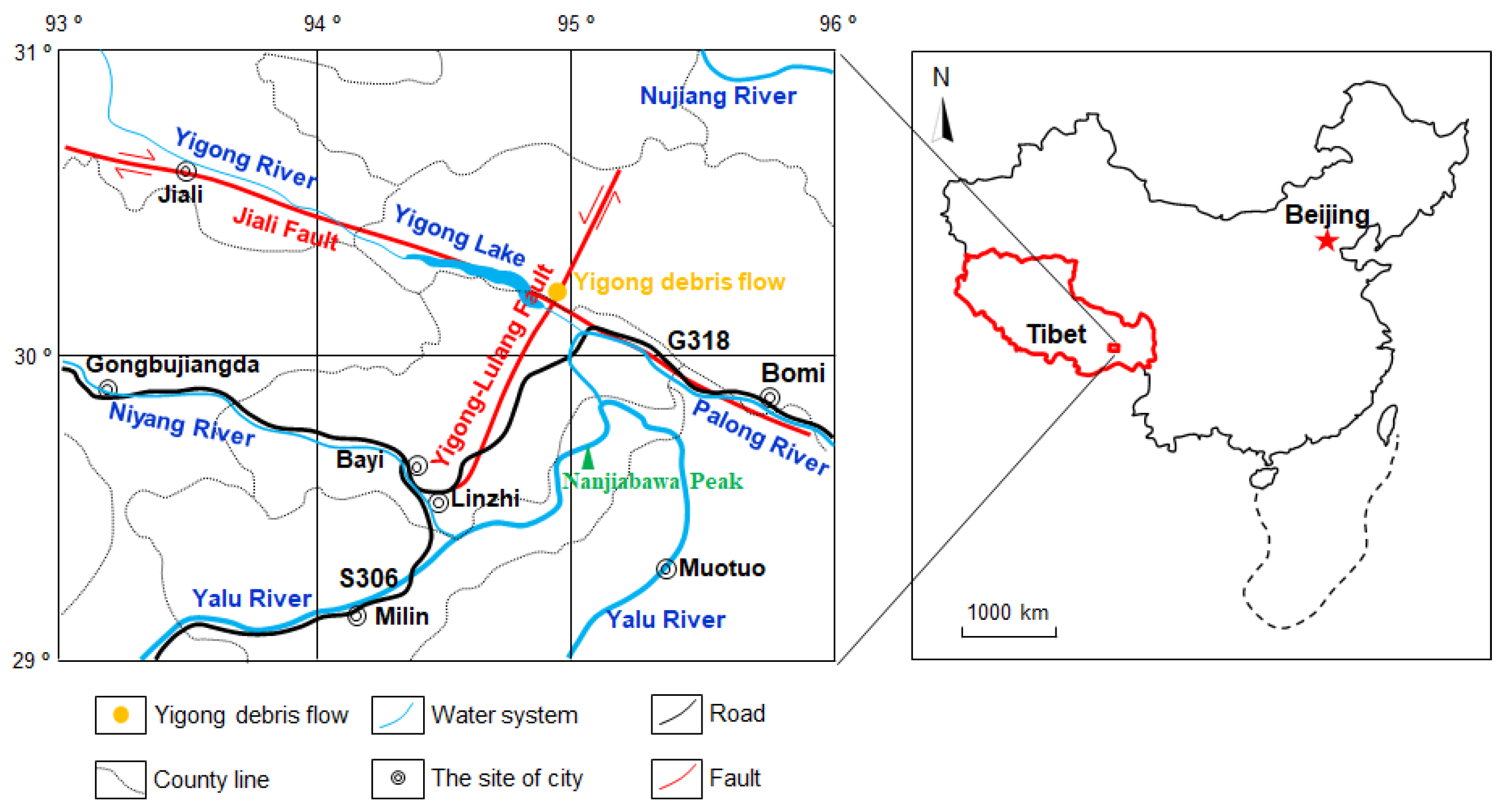
On 9 April 2000, a rock avalanche occurred at Zhamunong gully in Bomi County, southeastern Tibet, China. After detaching from the parent rock, it transformed to a high-speed and long-distance debris flow. The geographical coordinates of the debris flow are 30°12′11″ N, 94°58′03″ E [36]. Along the banks of Yigong river, the mountains are very high and steep, which are covered with thick snow over 4000 m and with dense vegetation below 3500 m. The valleys in this area are very deep under the erosions of glaciers and rivers.
The rock masses in the study area are mainly granitoid rocks, which have experienced strong weathering and have been partially metamorphosed into slate and granitic gneiss [37,38]. The surface of the slope is composed of quaternary loose colluvial deposits. Thick glaciers and snow covered the slope rock, which could decrease the shear strength of the geomaterial after melting and increase the weight of the sliding mass. Due to the collision between the Eurasian Plate and Indian Plate, active faults are well-developed in the Tibetan Plateau. Jiali Fault and Yigong-Lulang Fault, two of the major active strike-slip faults [39], meet at the mouth of Zhamunong gully, as shown in Figure 1. Earthquakes frequently occurred in the study area. For example, 14 moderate earthquakes (Ms = 4.0–5.9) were recorded around the Yigong lake from 1980 to 1996. Therefore, the tectonic activities in this area caused the rock structure fractured, loosened, and weakened, which provided favorable conditions for the Yigong debris flow occurrence.
The study area belongs to the temperate subhumid plateau monsoon climate area. Influenced by the warm–wet air currents from the Indian Ocean, the weather is humid, with clear four seasons and abundant in rainfall and sunshine. According to the local meteorological station, the annual rainfall averages 876.9 mm, and the cumulative sunshine hours is 1544 h. It was reported that the antecedent precipitation from 1 to 9 April 2000 was 42.9 mm, which was a main trigger of the debris flow. According to the three weather stations around Yigong area, the mean ground surface temperature in this area gradually increased before the occurrence of the Yigong debris flow [40]. It might result in the glacier melting in the source area and, thus, may have increased the pore water pressure in the geomaterials and decreased the shear strength.
2.2. Debris Flow Features
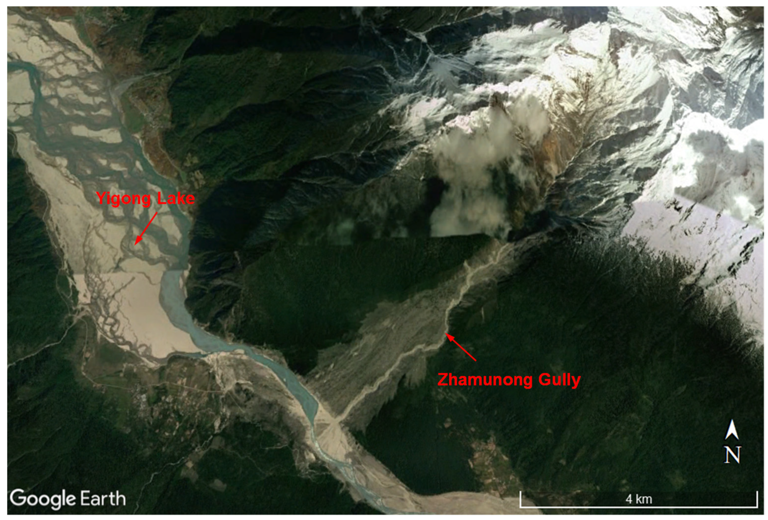
Figure 2 shows an aerial view of the Yigong debris flow occurred in Zhamunong gully (the base map is taken from Google Earth). About 3.0 × 10⁸ m3 geomaterials slid down along the gully for about 3 min [36,37], and the sliding direction is around 225°. The horizontal runout distance is about 8000 m, and the vertical dropdown is about 3330 m from its source area at 5520 m to its sediment fan at 2190 m. Deduced from seismic surveillance data, the maximum velocity of the debris flow is higher than 100 m/s, and the average velocity is about 40 m/s [40,41].
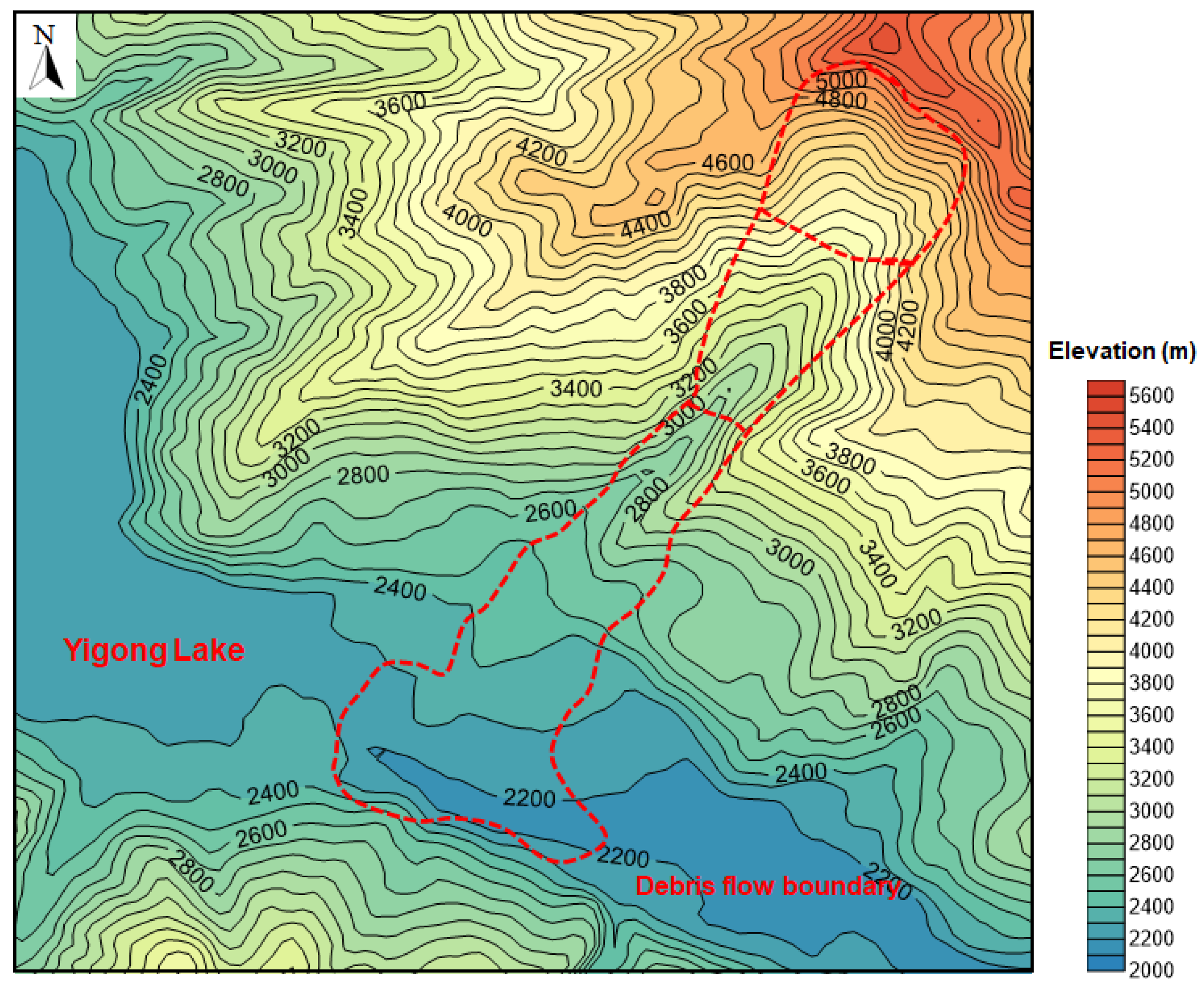
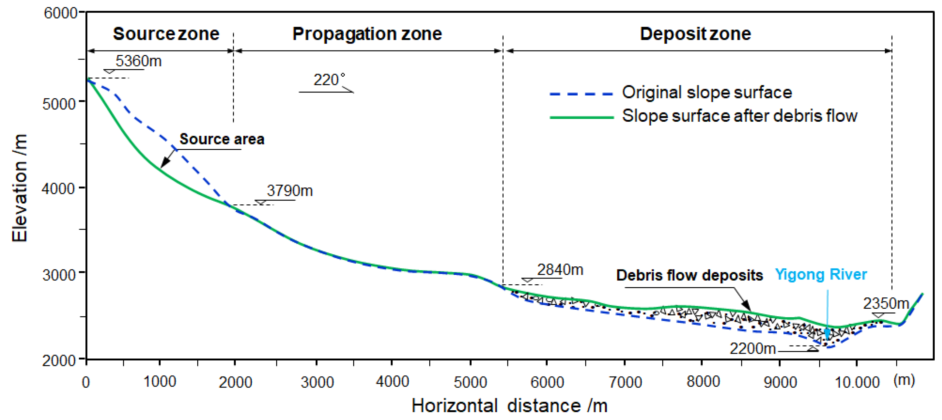
Figure 3 is the topographic contour map of the Yigong debris flow. The red dashed line shows the disaster boundary, and the total surface area of this debris flow was about 12.9 km2. The elevation of the debris flow top is about 5360 m, and the lowest elevation of the deposit area is about 2200 m. The slope at both sides of the Zhamunong gully are very steep. Figure 4 shows the path profile of this debris flow. In this figure, the original slope surface (blue dashed line) and the present slope surface (green solid line) are from [42]. As shown in Figure 4, the debris flow could be identified by three major zones: source zone, propagation zone, and deposit zone. The characteristics of the three zones are described below.
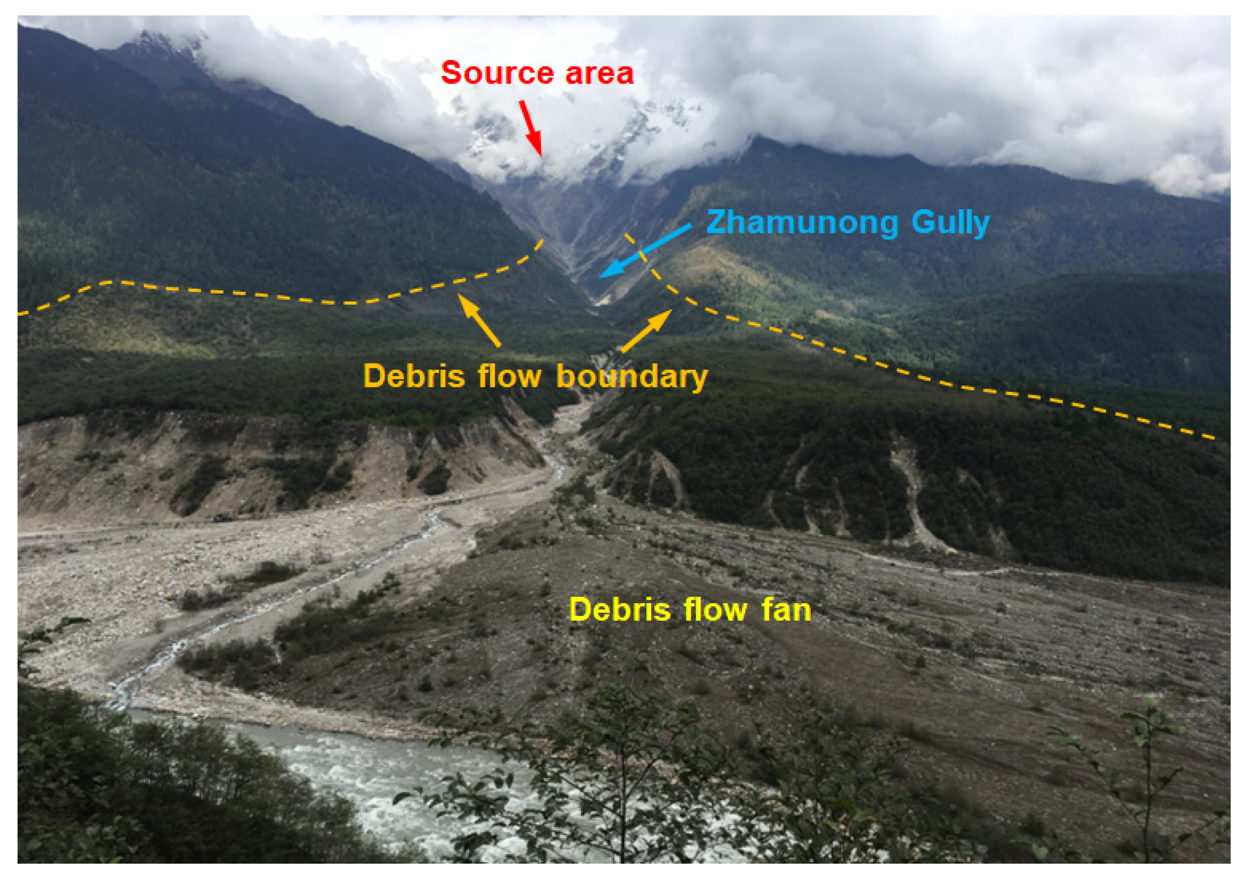
2.2.1. Source Zone
Figure 5 shows an oblique view of the source zone of the Yigong debris flow, which is located at the top of the Zhamunong gully. It covered an area of about 1.40 km2. The elevation of the source area sharply decreased from 5360 to 3750 m, with a slope angle of 40.0°. This area was covered by thick glaciers almost all year round. The source area was wedge-shaped, wide at the top and narrow at the bottom. It poured down along the creek bed at a high speed.
2.2.2. Propagation Zone
The propagation zone of this debris flow covered an area of about 3.46 km2. The axial length of this zone is about 3200 m, and the width ranges from 780 to 1500 m. The elevation of this zone ranges from 3790 to 2840 m, with a height difference of 950 m. The average slope of this zone is about 16.0°, which was much gentler than that of the source zone. Many boulders are distributed in the gully. Most of these are angular with a diameter of over 0.5 m.
2.2.3. Deposit Zone
Figure 6 is the front view of the deposit zone of the Yigong debris flow. The elevation of this zone ranges from 2200 to 2800 m, and the average slope is about 6.0°. The area of the debris flow deposition is about 5.0 × 10⁶ m2, and the average depth of sediment is about 50 m [3]. Due to the high motion velocity, the debris flow flushed into the Yigong river and formed a huge dam and an extensive dammed lake. The location of the lake is shown in Figure 2. The length of the trumpet-shaped dam is about 4.6 km, the maximum width is 3.0 km, and the dam height is 60–120 m. The dam sloped at 5° at the upstream side and 8° at the downstream side [35]. After the dam formation, water level of the Yigong lake continuously rose at a rate of about 1 m/day, which flooded the Yigong tea farm, schools, and villages surrounding the barrier lake. On 10 June 2000, the dam failed and resulted in devastating flooding, which destroyed farms, villages, bridges, and highways along its route. In recent years, the loose sediment was eroded by water from the Zhamunong gully and formed a debris fan in the Yigong river channel.
3. Numerical Model
To investigate the kinetic characteristics of the Yigong debris flow, a meshfree numerical method named smoothed particle hydrodynamics (SPH) is applied, and two-dimensional and three-dimensional models were established for the rapid debris flow propagation simulation.
3.1. SPH Algorithm
The SPH method was proposed in 1997 for astrophysical applications [43]. Recently, this method has been widely applied to a large variety of engineering fields [44,45,46,47]. Compared to the mesh-based method, the major advantage of the SPH method is to bypass the need for numerical meshes and avoid the mesh distortion issue and a great deal of computational work to renew the mesh [48].
In the SPH method, the subject is represented by a set of particles to which the material properties such as velocity, density, and pressure are associated. The properties are updated for each time step of the simulation following the conservation laws of mass and momentum [49].
In this study, the debris flow is assumed as a kind of weakly compressible viscous fluid. Therefore, the continuity and momentum equations are expressed by:
where ρ is the particle density, t is the time, and m is the particle mass, v is the velocity, p is the pressure, and F is the body force. The subscripts i and j are the concerning particle and its neighboring particle. δ is the Kronecker delta and Π is an artificial viscosity, which is used to improve the stability of the numerical results [50]. W is a smooth function. In this model, the cubic B-spline function, originally used by Monaghan and Lattanzio [50], is selected as the smooth function. The function formula is
where αd is a normalization factor in two- and three-dimensional space, αd = 15/7 πh2 and 3/2 πh3, respectively. R is the normalized distance between particles i and j, defined as R = r/h. Here, r is the distance between particles i and j.
The pressure p can be calculated by an equation of state in this study:
where ρ is the density calculated by the continuity equation, see Equation (1). ρ0 is the reference density which can be measured through laboratory tests. cs is the sound speed at the reference density, which can be set equal to ten times the maximum velocity [51]. γ is the exponent of the equation of state and is usually set to 7.0 for a good simulation of geomaterial flow behavior [52].
3.2. SPH Model of the Yigong Debris Flow
3.2.1. Material Model
The debris flow mass is a mixture of water, soil, and rock, which is complicated to describe. Hungr [53] proposed a concept of “equivalent fluid”, which was intended to simulate the bulk behavior of the debris flow mass. Rickenmann et al. [54] used three different fluid models based on Voellmy fluid rheology, quadratic rheology, and Herschel–Bulkley rheology to simulate the propagation of debris flows across two-dimensional terrain. Recently, some viscous fluid models have been widely used in the numerical modeling of debris flows [29,55,56]. In the presented SPH model, the debris flow mass is assumed as a Bingham fluid, which is widely used to describe the motion behavior of debris flows because of its simple structure [57,58]. The relationship between the shear stress and the shear strain rate in the Bingham fluid model is defined as
where τ is the shear stress of the fluid, η is the yield viscosity coefficient in fluid dynamics, and τy is the yield shear stress, which is commonly defined as the Mohr–Coulomb yield criterion with the cohesion c and frictional angle φ [29,59]. p is the pressure which can be obtained by Equation (3). D and DΠ are the strain rate and its second invariant.
3.2.2. Boundary Treatment
SPH method is ideal to deal with the free surface boundary. In the presented model, the free surface is identified through the criterion below:
where ρ* is present value of the particle density, which equals the initial density ρ0 plus the density increment dρ. The density increment dρ can be obtained according to the mass conservation equation, as shown in Equation (1). k is the free surface parameter. When the particle is identified as a free boundary particle, then zero pressure is applied.
For the solid wall boundary, ghost particles are placed on the boundary lines to exert repulsive forces and avoid the particles crossing the boundary. The velocities of the ghost particles are set to be zero to satisfy the non-slip boundary condition. For a detailed description of the non-slip boundary condition, please refer to [44].
3.2.3. OpenMP Parallelism
To simulate the propagation of a debris flow across complex terrain, it is necessary to develop a three-dimensional numerical model. In the 3D SPH model, however, the computational efficiency is sharply reduced as the particle number increases. To improve the efficiency, it is necessary to parallelize the numerical code without suffering from a loss of precision.
The open multiprocessing (OpenMP) API for shared-memory programming enables loop-level parallelism by the insertion of pragmas within the source code. By adding special directives at the beginning and end of the loop, OpenMP parallel implementation can be easily conducted. The cycles of the loop are then randomly assigned to the available threads. In the present work, the paralleled numerical code was written in FORTRAN 95, and the program was compiled using Microsoft Visual studio 2015 in a PC with the quad-core 8-thread CPU, Intel Core i7-7820HQ, and run at 2.90 GHz clock with 32 GB main memory under the Windows 10 Professional 64-bit operating system.
3.2.4. Time Integration
In a Lagrangian framework, the coordinates of each particles are updated at each time steps. A velocity Verlet scheme is introduced in this SPH model to perform time integration.
where X, V, and a are the displacement, velocity, and acceleration field, respectively.
4. Kinetic Characteristics of the Yigong Debris Flow
4.1. Two-Dimensional Modeling
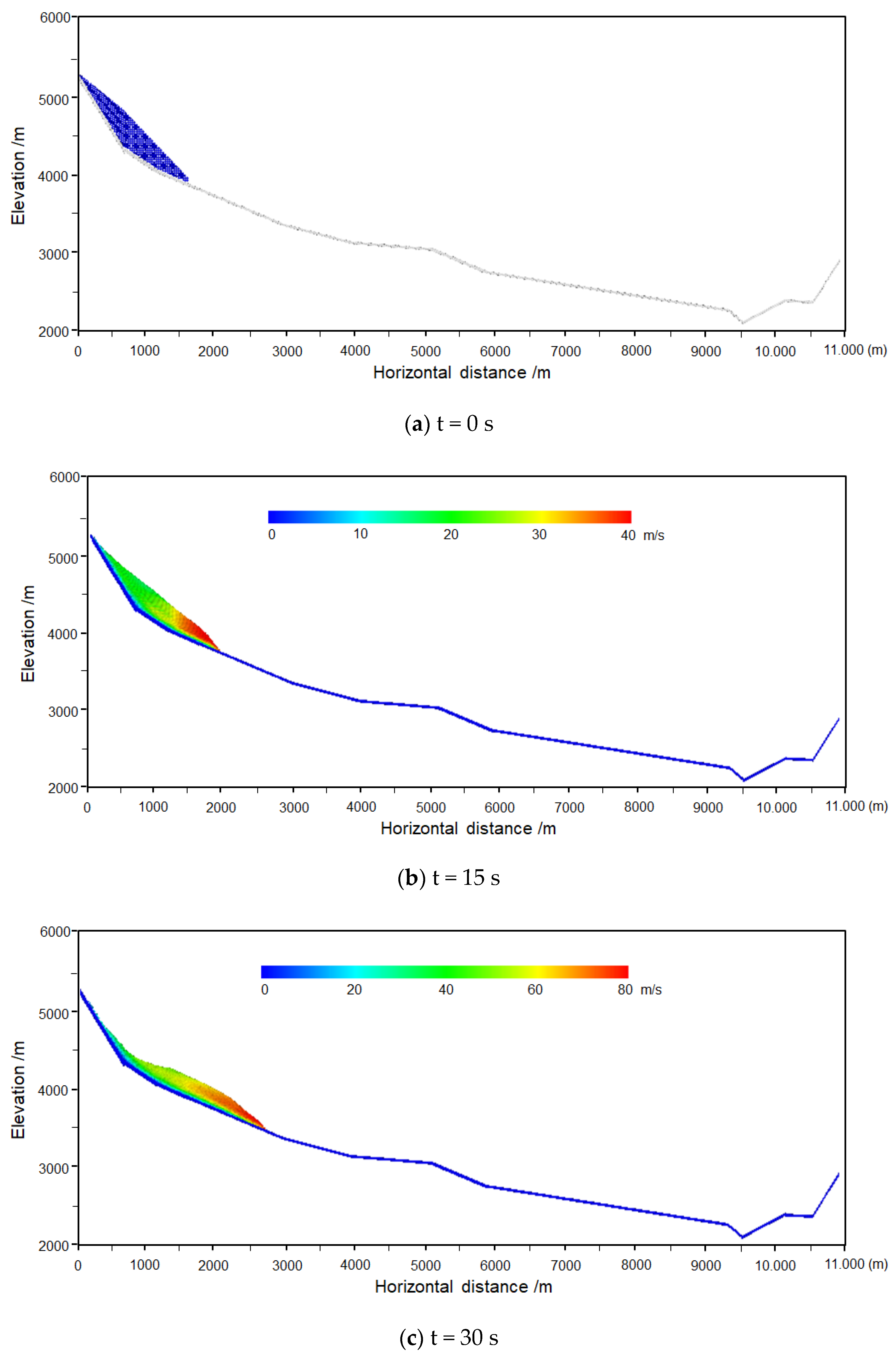
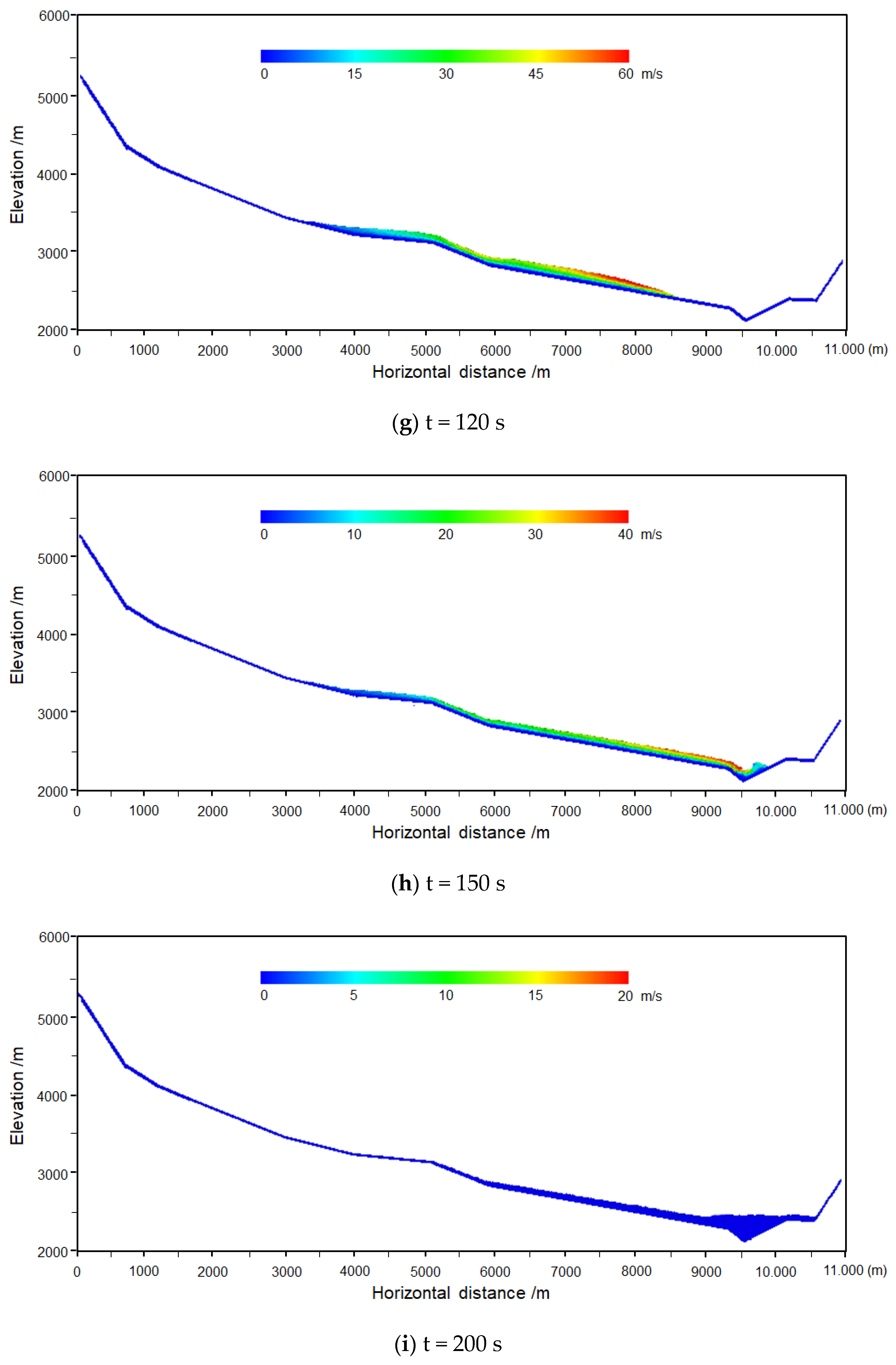
According to the debris flow profile in Figure 4, a two-dimensional SPH model was established in this study to simulate the flow behavior of the Yigong debris flow, as shown in Figure 7a. The number of SPH particles used in the numerical model can simultaneously influence the computational efficiency and accuracy [49]. Therefore, to reach an appropriate balance between the computational efficiency and accuracy, 7662 blue particles were used to represent the debris flow mass, and 5906 grey image particles were used to simulate the bed surface. The diameters of those particles are 8 m. The initial velocities of the particles were set to zero. After slope failure, the debris flow mass particles slide down the slope under the action of gravity, while the boundary particles remain stationary throughout the simulation. According to Li et al. [60], the average density of the Yigong debris flow mass was about 2000 kg/m3. The strength characteristics of the debris flow mass were studied through a series of high-speed ring shear tests and rotary shear tests in the previous studies [61,62]. According to the test results, the values of the c and φ of the geomaterial can be approximately set to be 10 kPa and 20°, respectively. The selection of dynamic viscosity η is often challenging. In the previous simulation, Bingham model was widely used to simulate debris flows considering a range of dynamic viscosities from 20 to 500 Pa·s [29,63,64]. The sound speed cs is set to be 10 vmax (vmax is the maximum velocity). The parameter γ in the equation of state is set to be 7.0 for a good simulation of geomaterial flow behavior.
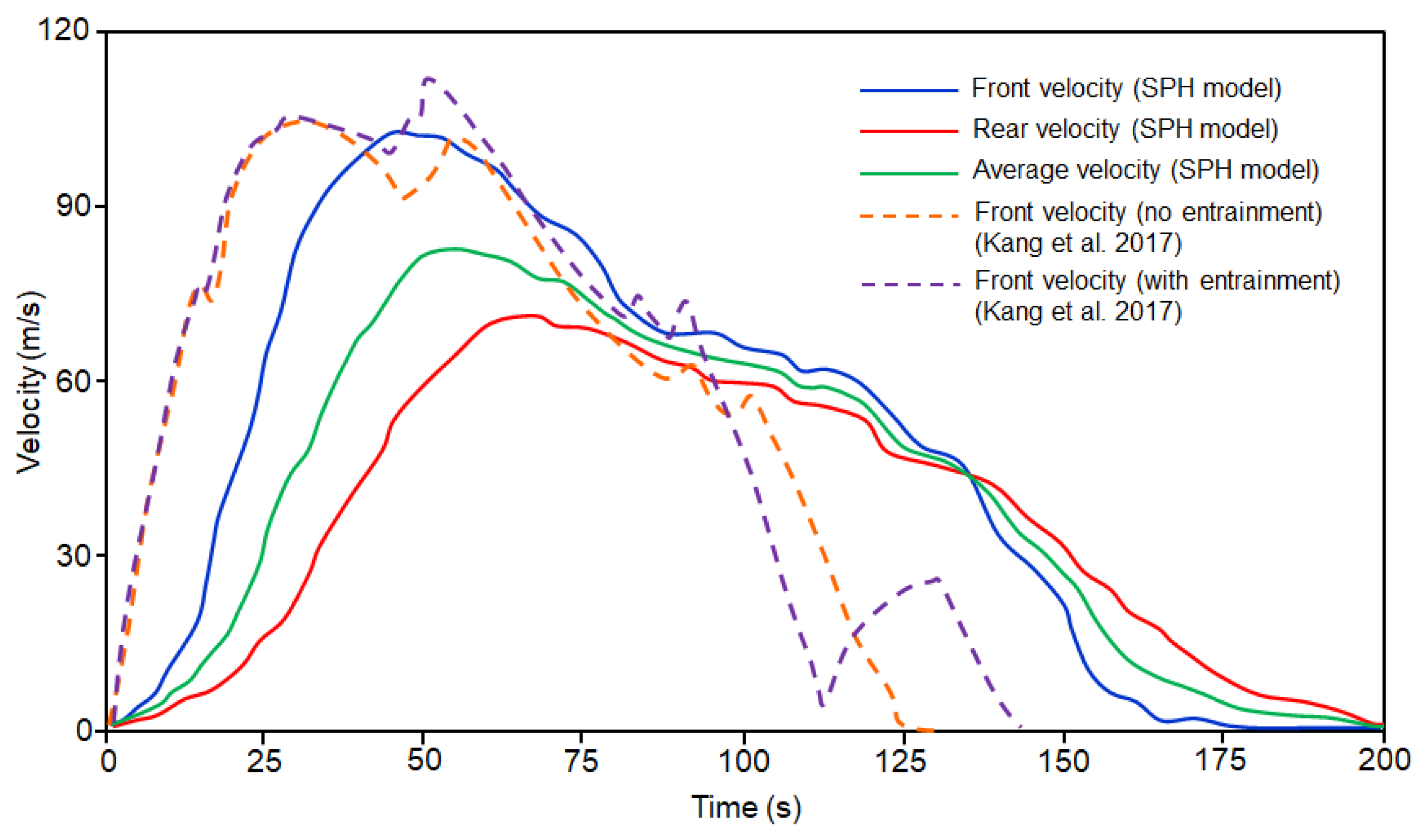
According to the simulation results, the motion process of the debris flow mass takes about 200 s, which is basically consistent with the witnesses’ description [36]. Figure 7 presents the slope configurations at different points in time, which indicates the motion process of the debris flow mass after slope failure. The particles slide down from the top of the Zhamunong gully, and then move along the steep slope by gravity. Finally, these particles run to an equilibrium state and accumulate in the Yigong river channel. The color represents the velocity of the particles, which shows that the maximum flow velocity of the debris flow mass is about 100 m/s. To investigate the kinetic characteristics of the debris flow, Figure 8 shows the time history curves of the flow velocity. The blue, red, and green curves represent the velocity evolutions of the rear edge, front edge, and the average value of the debris flow mass. The peak velocities are 102.6 m/s at the front edge and 72.4 m/s at the rear edge. The average velocity of the debris flow mass during the propagation is approximately 39.8 m/s. After slope failure, debris flow mass rapidly slides down and accelerates due to gravity. In this stage, most of the potential energy of the debris flow mass is converted into kinetic energy. After the peak velocity, the kinetic energy is consumed due to the friction, collision, and the breakage of the sliding mass, and the velocity gradually decreases. The overall performance of the sliding mass is accelerated motion in the period 0–50 s and decelerated motion after 50 s.
In Figure 8, the orange and purple dashed lines are the time history curves of the front velocity obtained by the energy models with and without bed entrainment proposed by Kang et al. (2017). The comparison results show that the variation tendencies of the debris flow velocity obtained by the SPH model and the energy models are similar, and the maximum front velocities are also very close. However, the motion time of the debris flow simulated by SPH model is a bit longer than that simulated by the energy models.
Figure 9 compares the simulated debris flow deposition with the measured data recorded in [42]. It is obvious that the predicted debris flow deposition area is consistent with the measured data. In order to identity the influence degree of each rheological parameter on the numerical results, sensitivity analysis was conducted by varying the rheological parameters. Table 1 lists the seven calculation cases with different rheological parameters. To explicitly quantify the differences between measured and calculated deposits, the L2 relative error norm in the deposition depth, εL2, was evaluated using the following equation:
where Y is the measured deposition depth, ΔY is the deviation of numerical and measured depth, and N is the total number of points at which the depths are compared. As shown in Figure 9, a total of 11 points with a space of 500 m were selected to calculate the error norm, and the results of all the seven cases are listed in Table 1, which shows that the coefficient of viscosity has more influence on the computing accuracy in comparison with the shearing strength parameters.
4.2. Three-Dimensional Modeling
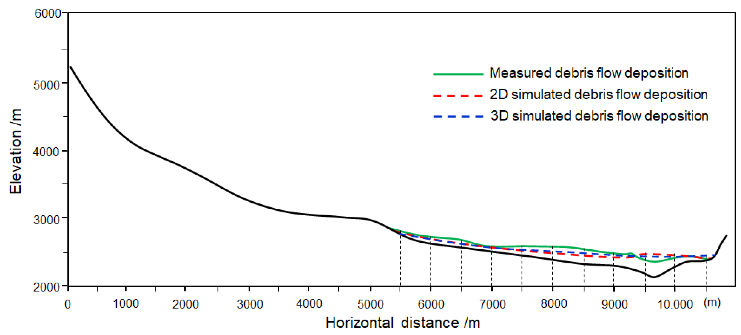
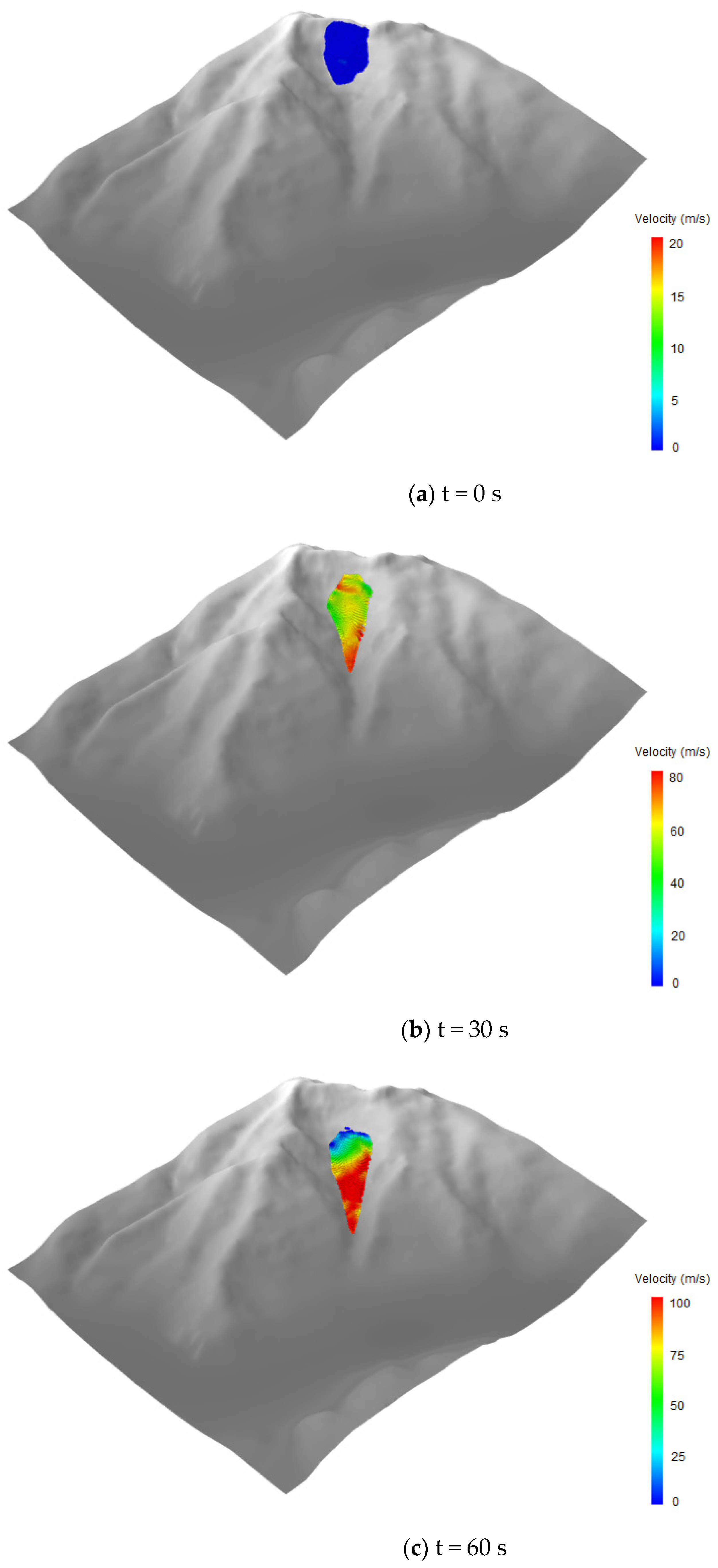
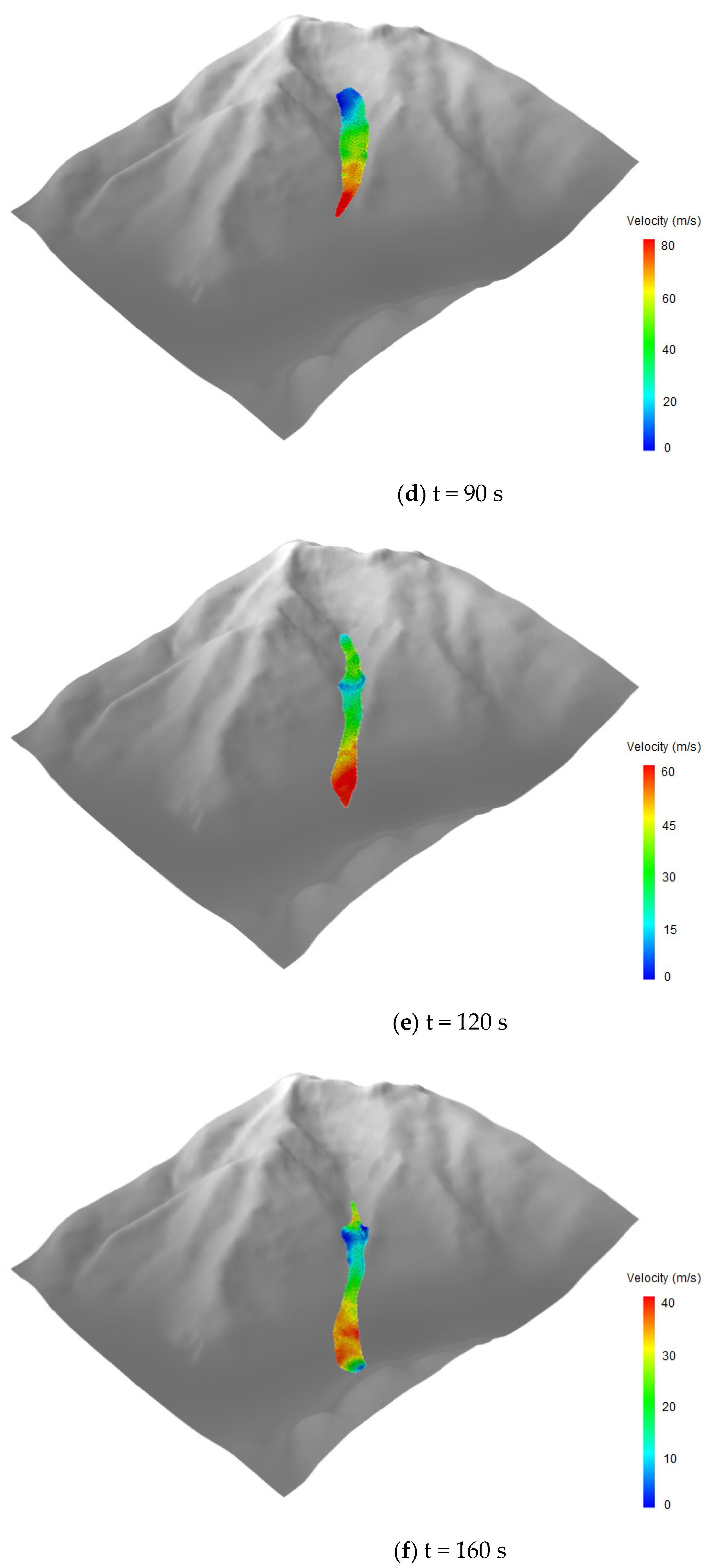
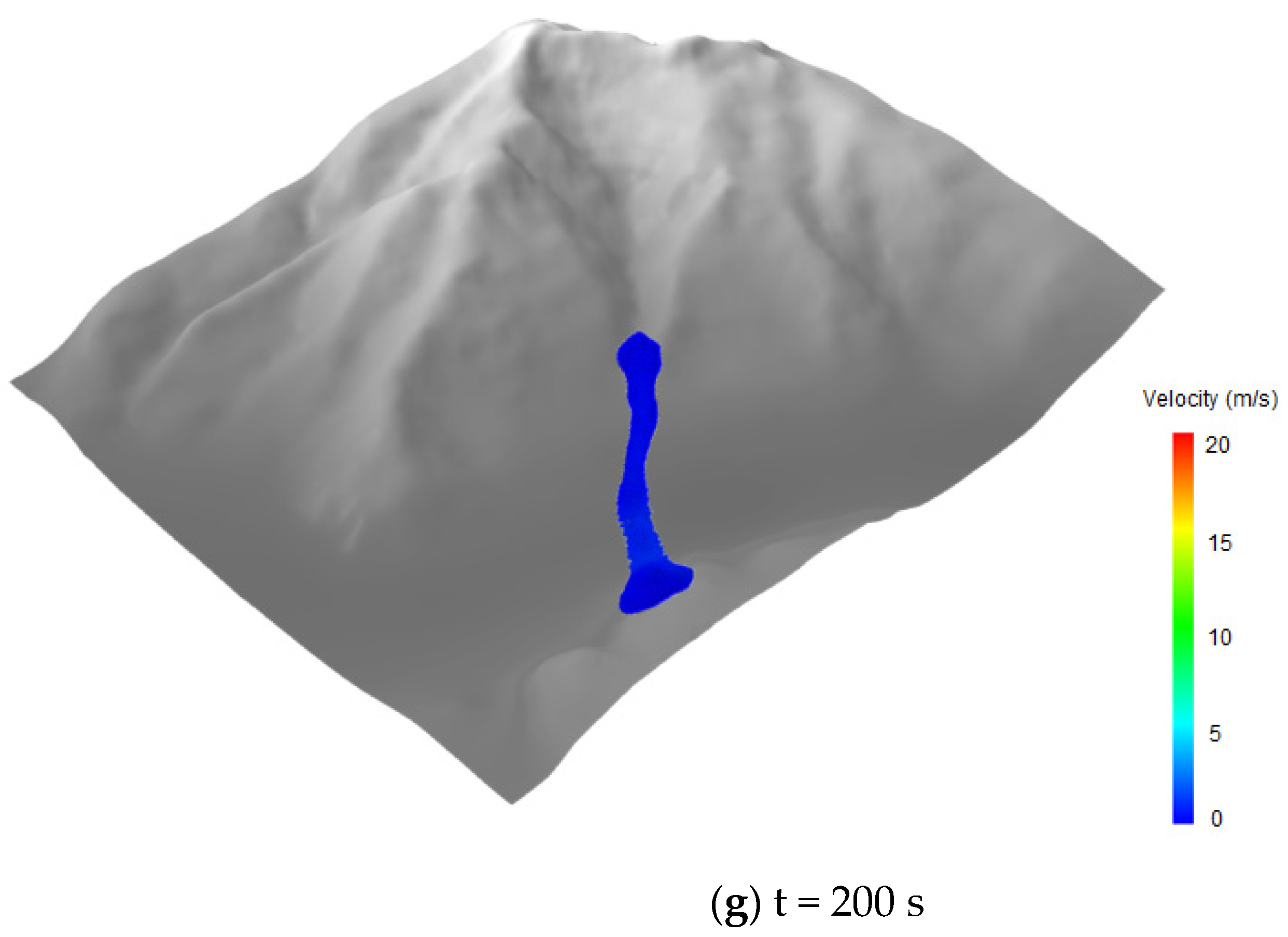
To simulate the debris flow propagation across 3D complex terrain, the 2D SPH model is developed into a 3D version. In the 3D model, the diameter of the SPH particles is set to be 20 m since the resolution of the digital elevation model (DEM) is 20 m × 20 m. The debris flow mass in the source area is discretized into about 11,000 particles so that the total volume of the debris flow is about 3.0 × 10⁸ m3. The number of particles along the vertical direction varies in different positions according to the depth of the sliding surface at that position. The strength parameters used in 3D simulation are the same as those used in 2D model. Based on this model, the numerical modeling of the Yigong debris flow motion across 3D terrain is conducted, and the results are shown in Figure 10. The color of the particles in the figures represents the sliding velocity. After slope failure, the debris flow mass goes through an acceleration process since the slope is quite steep in the source area. The maximum sliding velocity is about 98.4 m/s, which appears at 47.5 s after the slope failure. Afterwards, the debris flow mass slows down gradually due to the friction and the collision during the propagation. Finally, the debris flow mass crashes into a mountain on the opposite bank of Yigong river and then blocks the river channel. The whole motion process takes about 200 s, and the final depositions of the debris flow mass on the runout path are shown in Figure 10g. Figure 11 shows the Yigong debris flow deposition. The red dashed line is the simulated debris flow deposition, with the area of 4.76 km2, which is close to the measured data 5.0 km2 [37]. The maximum length and width of the deposition belt are 4.62 and 2.84 km, respectively, which are close to the observed values of 4.60 and 3.0 km, and its shape is basically in agreement with the observed shape (blue solid line in Figure 11).
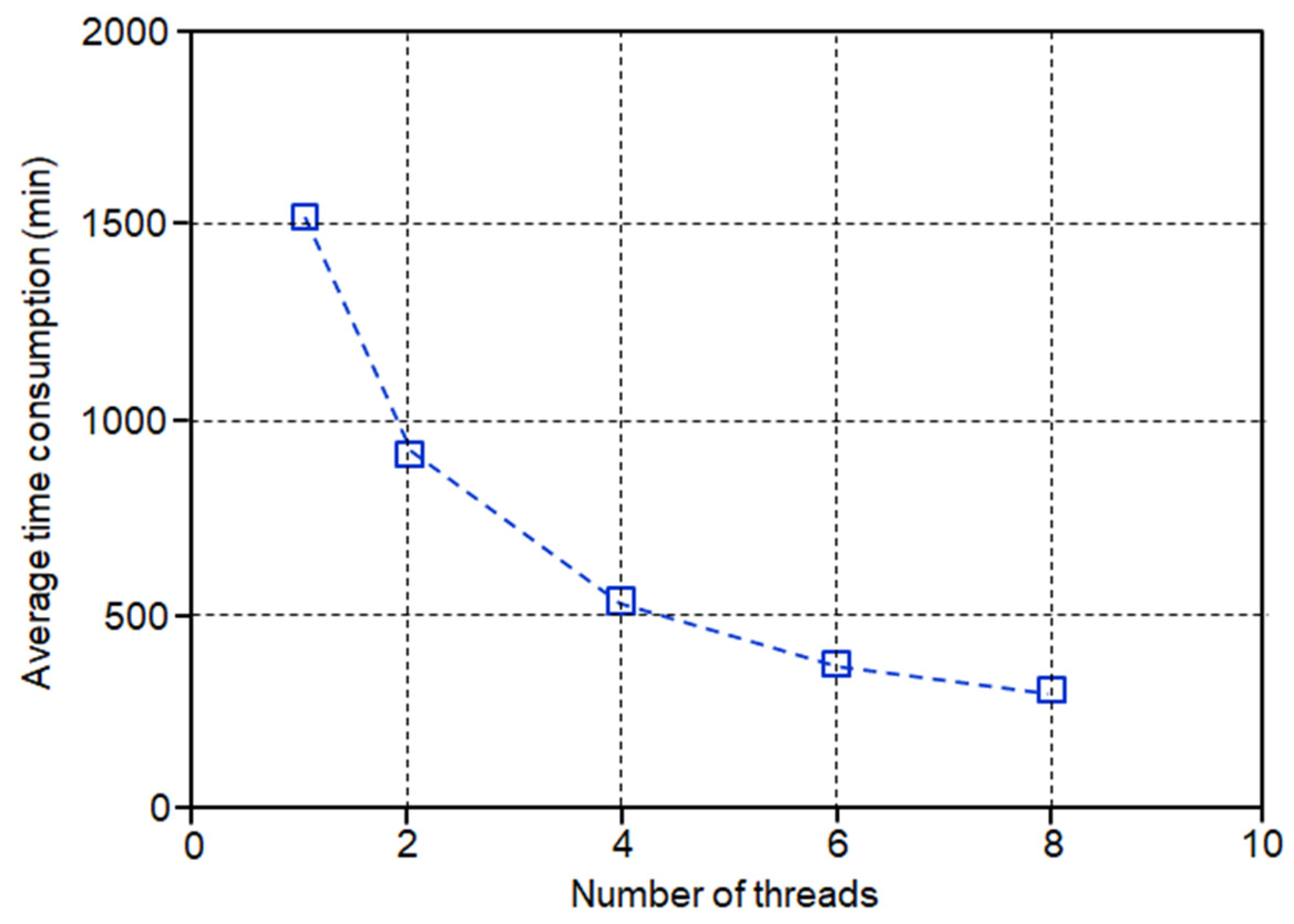
To verify the performance of parallel computation, the 3D SPH modeling was carried out using different thread numbers (1, 2, 4, 6, and 8). Figure 12 shows the relationship between the average program running time and the thread number. It is obvious that the computation efficiency of the presented SPH model increases with the thread number.
4.3. Analysis of Simulation Results
Runout distance, deposition area, and deposition depth are very important for debris flow disaster prediction. About two months after the Yigong debris flow occurrence, the dam broke down, and most of the debris flow deposit was washed away by the flood. Therefore, it is difficult to measure the post-event topography in the field. In this study, the SPH modeling results showed that the total runout distance of the Yigong debris flow was about 8000 m, which are consistent with the measured results [40]. The final deposition area was obtained by 3D SPH modeling, which is in correspondence with the satellite image provided in [65]. The 2D simulated deposition depths along the topographic profile can match the observed results provided in [42] well, while in the 3D modeling, the comparative analysis of deposition depths was not carried out due to lack of measured data.
Velocity is one of the key kinetic characteristics during debris flow propagation, which is difficult to measure in field. According to eyewitness accounts, the total sliding time of the Yigong debris flow was about 3 min. The runout distance was about 8000 m. Therefore, the average flow velocity of the debris flow was estimated to be about 40 m/s. According to the dynamic analysis results [40,60], the maximum velocity during the debris flow propagation was more than 100 m/s. Therefore, the velocity–time history predicted by the SPH model in this work fits the literature data well and is reasonable and reliable.
During debris flow propagation, bed entrainment can increase the source volume and then affect the kinematic characteristics. Recently, several numerical models regarding bed entrainment have been proposed with some satisfactory results [36,40]. However, due to many influencing factors, such as particle shape and gradation, pore water pressure, thickness, and compactness of the bed material, it is quite difficult to effectively incorporate the entrainment algorithm into the presented SPH model. In spite of this imperfection, the SPH model presented in this study can simulate the kinetic characteristics of the Yigong debris flow and reach a certain accuracy.
5. Conclusions
All over the world, debris flows always lead to property loss and human death. This work investigates the kinetic features of the catastrophic Yigong debris flow in the Tibetan Plateau, China. On the basis of the SPH method, 2D and 3D numerical simulations were conducted to reproduce the motion process of the Yigong debris flow. Based on the numerical results and combined with field investigation data and remote-sensing images, the kinetic characteristics of the debris flow were analyzed. Some conclusions can be obtained as below.
In the early stage, debris flow mass slides down along the deep slope in the source area. It experiences an acceleration and reaches its peak velocity (about 100 m/s). In this stage, most of the potential energy of the debris flow mass is converted into kinetic energy. During debris flow propagation in the Zhamunong gully, the kinetic energy continuously dissipates due to the friction and the collision. The velocity gradually slows down in this stage. After rushing out of the Zhamunong gully, the debris flow mass crashes into a mountain on the opposite bank of Yigong river and then blocks the river channel. The velocity evolution of the debris flow is obtained based on numerical results, and the final debris flow deposition is predicted, which basically fits the measured data in field.
Although the SPH model presented in this work can reproduce the motion process and analyze the kinetic characteristics of the Yigong debris flow, there are still some problems need to be solved. For example, the bed material entrainment during debris flow propagation has some effect on the debris flow volume and its kinetic characteristics, but was not considered in this work. On the other hand, the disintegration and fragmentation of the rock blocks was not considered in the presented SPH model, which may lead to some error during the simulation of debris flow propagation. Moreover, high-performance parallel computing technology is necessary to improve the calculation efficiency in 3D modeling.
Author Contributions
Conceptualization, Z.D. and S.Q.; methodology, Z.D. and S.Q.; investigation, Z.D., H.Y., and K.X.; writing—original draft preparation, Z.D., S.Q. and K.X.; writing—review and editing, S.Q.; visualization, K.X.; supervision, F.W. and S.Q.; funding acquisition, Z.D., F.W. and H.Y. All authors have read and agreed to the published version of the manuscript.
Funding
This research was funded by the Program for Professor of Special Appointment (Eastern Scholar) at Shanghai Institutions of Higher Learning, National Natural Science Foundation of China (grant No. 41807248, and grant No. 41530639).
Institutional Review Board Statement
Not applicable.
Informed Consent Statement
Not applicable.
Data Availability Statement
The data presented in this study are available on request from the corresponding author.
Acknowledgments
We are grateful to Q.G. Cheng, Y.F. Wang, and K.M. Yan for their great help in the field investigation.
Conflicts of Interest
The authors declare no conflict of interest.
References
- Zou, Q.; Cui, P.; Jiang, H.; Wang, J.; Li, C.; Zhou, B. Analysis of regional river blocking by debris flows in response to climate change. Sci. Total Environ. 2020, 741, 140262. [Google Scholar] [CrossRef] [PubMed]
- Huang, R.Q. Large-scale landslides and their sliding mechanisms in China since the 20th century. Chin. J. Rock Mech. Eng. 2007, 26, 433–454, (In Chinese with English abstract). [Google Scholar]
- Shang, Y.J.; Yue, Z.Q.; Yang, Z.F.; Wang, Y.C.; Liu, D.A. Addressing severe slope failure hazards along Sichuan-Tibet highway in southwestern China. Epis. Newsmag. Int. Union Geol. Sci. 2003, 26, 94–104. [Google Scholar]
- Zou, Z.X.; Tang, H.M.; Xiong, C.R.; Su, A.J.; Criss, R.E. Kinetic characteristics of debris flows as exemplified by field investigations and discrete element simulation of the catastrophic Jiweishan rockslide, China. Geomorphology 2017, 295, 1–15. [Google Scholar] [CrossRef]
- Leonardi, A.; Pirulli, M. Analysis of the load exerted by debris flows on filter barriers: Comparison between numerical results and field measurements. Comput. Geotech. 2020, 118, 103311. [Google Scholar] [CrossRef]
- Liu, S.L.; Zhang, J.C.; Cheng, X.; Wang, W.B.; Jiang, H.T. Gradation and Rheological Characteristics of Glacial Debris Flow along the Kangding-Linzhi Section of Sichuan-Tibet Railway. Adv. Civ. Eng. 2020, 2020, 8886137. [Google Scholar]
- Chang, M.; Liu, Y.; Zhou, C.; Che, H.X. Hazard assessment of a catastrophic mine waste debris flow of Hou Gully, Shimian, China. Eng. Geol. 2020, 275, 105733. [Google Scholar] [CrossRef]
- Ma, C.; Deng, J.Y.; Wang, R. Analysis of the triggering conditions and erosion of a runoff-triggered debris flow in Miyun County, Beijing, China. Landslides 2018, 15, 2475–2485. [Google Scholar] [CrossRef]
- Xiong, J.; Tang, C.; Chen, M.; Zhang, X.Z.; Shi, Q.Y.; Gong, L.F. Activity characteristics and enlightenment of the debris flow triggered by the rainstorm on 20 August 2019 in Wenchuan County, China. Bull. Eng. Geol. Environ. 2021, 80, 873–888. [Google Scholar] [CrossRef]
- Fannin, R.J.; Wise, M.P. An empirical-statistical model for debris flow travel distance. Can. Geotech. J. 2001, 38, 982–994. [Google Scholar] [CrossRef]
- Tang, C.; Zhu, J.; Chang, M.; Ding, J.; Qi, X. An empirical-statistical model for predicting debris-flow runout zones in the Wenchuan earthquake area. Quat. Int. 2012, 250, 63–73. [Google Scholar] [CrossRef]
- Huang, J.; Hales, T.C.; Huang, R.Q.; Ju, N.P.; Li, Q.; Huang, Y. A hybrid machine-learning model to estimate potential debris-flow volumes. Geomorphology 2020, 367, 107333. [Google Scholar] [CrossRef]
- Fang, Q.S.; Tang, C.; Chen, Z.H.; Wang, S.Y.; Yang, T. A calculation method for predicting the runout volume of dam-break and non-dam-break debris flows in the Wenchuan earthquake area. Geomorphology 2019, 327, 201–214. [Google Scholar] [CrossRef]
- Zhou, G.G.D.; Li, S.; Song, D.R.; Choi, C.E.; Chen, X.Q. Depositional mechanisms and morphology of debris flow: Physical modelling. Landslides 2019, 16, 315–332. [Google Scholar] [CrossRef]
- Wang, D.P.; Chen, Z.; He, S.M.; Chen, K.J.; Liu, F.M.; Li, M.Q. Physical model experiments of dynamic interaction between debris flow and bridge pier model. Rock Soil Mech. 2019, 40, 3363–3372. [Google Scholar]
- Tan, D.Y.; Yin, J.H.; Qin, J.Q.; Zhu, Z.H.; Feng, W.Q. Experimental study on impact and deposition behaviours of multiple surges of channelized debris flow on a flexible barrier. Landslides 2020, 17, 1577–1589. [Google Scholar] [CrossRef]
- Brighenti, R.; Spaggiari, L.; Segalini, A.; Savi, R.; Capparelli, G. Debris flow impact on a flexible barrier: Laboratory flume experiments and force-based mechanical model validation. Nat. Hazards 2021, 106, 735–756. [Google Scholar] [CrossRef]
- Bowman, E.T.; Laue, J.; Imre, B.; Springman, S.M. Experimental modelling of debris flow behaviour using a geotechnical centrifuge. Can. Geotech. J. 2010, 47, 742–762. [Google Scholar] [CrossRef]
- Milne, F.D.; Brown, M.J.; Knappett, J.A.; Davies, M.C.R. Centrifuge modelling of hillslope debris flow initiation. Catena 2012, 92, 162–171. [Google Scholar] [CrossRef]
- Zhou, J.W.; Cui, P.; Yang, X.G. Dynamic process analysis for the initiation and movement of the Donghekou landslide-debris flow triggered by the Wenchuan earthquake. J. Asian Earth Sci. 2013, 76, 70–84. [Google Scholar] [CrossRef]
- Chen, R.D.; Liu, X.N.; Cao, S.Y.; Guo, Z.X. Numerical simulation of deposit in confluence zone of debris flow and mainstream. Sci. China Technol. Sci. 2011, 54, 2618–2628. [Google Scholar] [CrossRef]
- Cascini, L.; Cuomo, S.; Pastor, M.; Rendina, I. SPH-FDM propagation and pore water pressure modelling for debris flows in flume tests. Eng. Geol. 2016, 213, 74–83. [Google Scholar] [CrossRef]
- Shen, W.; Li, T.L.; Li, P.; Lei, Y.L. Numerical assessment for the efficiencies of check dams in debris flow gullies: A case study. Comput. Geotech. 2020, 122, 103541. [Google Scholar] [CrossRef]
- Lei, M.; Yang, P.; Wang, Y.K.; Wang, X.K. Numerical analyses of the influence of baffles on the dynamics of debris flow in a gully. Arab. J. Geosci. 2020, 13, 1052. [Google Scholar] [CrossRef]
- Zhou, G.G.D.; Du, J.H.; Song, D.R.; Choi, C.E.; Hu, H.S.; Jiang, C.H. Numerical study of granular debris flow run-up against slit dams by discrete element method. Landslides 2020, 17, 585–595. [Google Scholar] [CrossRef]
- Zhou, X.Y.; Sun, D.A.; Xu, Y.F. A new thermal analysis model with three heat conduction layers in the nuclear waste repository. Nucl. Eng. Des. 2021, 317, 110929. [Google Scholar] [CrossRef]
- Zhou, J.; Li, Y.X.; Jia, M.C.; Li, C.N. Numerical Simulation of Failure Behavior of Granular Debris Flows Based on Flume Model Tests. Sci. World J. 2013, 2013, 603130. [Google Scholar] [CrossRef] [Green Version]
- Dai, Z.L.; Huang, Y.; Cheng, H.L.; Xu, Q. SPH model for fluid–structure interaction and its application to debris flow impact estimation. Landslides 2017, 14, 917–928. [Google Scholar] [CrossRef]
- Huang, Y.; Cheng, H.L.; Dai, Z.L.; Xu, Q.; Liu, F.; Sawada, K.; Moriguchi, S.; Yashima, A. SPH-based numerical simulation of catastrophic debris flows after the 2008 Wenchuan earthquake. Bull. Eng. Geol. Environ. 2015, 74, 1137–1151. [Google Scholar] [CrossRef]
- Coussot, P.; Piau, J.M. A large-scale field coaxial cylinder rheometer for the study of the rheology of natural coarse suspensions. J. Rheol. 1995, 39, 105–124. [Google Scholar] [CrossRef]
- Pellegrino, A.M.; Di Santolo, A.S.; Schippa, L. The sphere drag rheometer: A new instrument for analysing mud and debris flow materials. Int. J. Geomate 2016, 11, 2512–2519. [Google Scholar] [CrossRef]
- Pellegrino, A.M.; Scotto di Santolo, A.; Schippa, L. An integrated procedure to evaluate rheological parameters to model debris flows. Eng. Geol. 2015, 196, 88–98. [Google Scholar] [CrossRef]
- Portilla, M.; Chevalier, G.; Hürlimann, M. Description and analysis of the debris flows occurred during 2008 in the Eastern Pyrenees. Nat. Hazards Earth Syst. Sci. 2010, 10, 1635–1645. [Google Scholar] [CrossRef] [Green Version]
- Han, Z.; Su, B.; Li, Y.; Wang, W.; Wang, W.; Huang, J.; Chen, G. Numerical simulation of debris-flow behavior based on the SPH method incorporating the Herschel-Bulkley-Papanastasiou rheology model. Eng. Geol. 2019, 255, 26–36. [Google Scholar] [CrossRef]
- Wang, Z.; You, Y.; Zhang, G.; Feng, T.; Liu, J.; Lv, X.; Wang, D. Superelevation analysis of the debris flow curve in Xiedi gully, China. Bull. Eng. Geol. Environ. 2021, 80, 967–978. [Google Scholar] [CrossRef]
- Xu, Q.; Shang, Y.; van Asch, T.; Wang, S.; Zhang, Z.; Dong, X. Observations from the large, rapid Yigong rock slide—debris avalanche, southeast Tibet. Can. Geotech. J. 2012, 49, 589–606. [Google Scholar] [CrossRef]
- Shang, Y.J.; Yang, Z.F.; Li, L.H.; Liu, D.; Liao, Q.L.; Wang, Y.C. A super-large landslide in Tibet in 2000: Background, occurrence, disaster, and origin. Geomorphology 2003, 4, 225–243. [Google Scholar] [CrossRef]
- Zhou, J.W.; Cui, P.; Hao, M.H. Comprehensive analyses of the initiation and entrainment processes of the 2000 Yigong catastrophic landslide in Tibet, China. Landslides 2016, 13, 39–54. [Google Scholar] [CrossRef]
- Lee, H.Y.; Chung, S.L.; Wang, J.R.; Wen, D.J.; Lo, C.H.; Yang, T.F.; Zhang, Y.; Xie, Y.; Lee, T.Y.; Wu, G.; et al. Miocene Jiali faulting and its implications for Tibetan tectonic evolution. Earth Planet. Sci. Lett. 2003, 205, 185–194. [Google Scholar] [CrossRef] [Green Version]
- Kang, C.; Chan, D.; Su, F.; Cui, P. Runout and entrainment analysis of an extremely large rock avalanche—A case study of Yigong, Tibet, China. Landslides 2017, 14, 123–139. [Google Scholar] [CrossRef]
- Li, J.; Chen, N.S.; Zhao, Y.D.; Liu, M.; Wang, W.Y. A catastrophic landslide triggered debris flow in China’s Yigong: Factors, dynamic processes, and tendency. Earth Sci. Res. J. 2020, 24, 71–82. [Google Scholar] [CrossRef] [Green Version]
- Yin, Y.P. Characteristics of Bomi–Yigong huge high speed landslide in Tibet and the research on disaster prevention. Hydrogeol. Eng. Geol. 2000, 4, 8–11, (In Chinese with English abstract). [Google Scholar]
- Gingold, R.A.; Monaghan, J.J. Smoothed particle hydrodynamics: Theory and application to non-spherial stars. Mon. Not. R. Astron. Soc. 1977, 181, 375–389. [Google Scholar] [CrossRef]
- Dai, Z.L.; Huang, Y.; Cheng, H.L.; Xu, Q. 3D numerical modeling using smoothed particle hydrodynamics of flow-like landslide propagation triggered by the 2008 Wenchuan earthquake. Eng. Geol. 2014, 180, 21–33. [Google Scholar] [CrossRef]
- Dai, Z.L.; Huang, Y.; Xu, Q. A hydraulic soil erosion model based on a weakly compressible smoothed particle hydrodynamics method. Bull. Eng. Geol. Environ. 2019, 78, 5853–5864. [Google Scholar] [CrossRef]
- Jamalabadi, M.Y.A. Frequency analysis and control of sloshing coupled by elastic walls and foundation with smoothed particle hydrodynamics method. J. Sound Vib. 2020, 476, 115310. [Google Scholar] [CrossRef]
- Price, D.J.; Laibe, G. A solution to the overdamping problem when simulating dust-gas mixtures with smoothed particle hydrodynamics. Mon. Not. R. Astron. Soc. 2020, 495, 3929–3934. [Google Scholar] [CrossRef]
- Ma, C.; Iijima, K.; Oka, M. Nonlinear waves in a floating thin elastic plate, predicted by a coupled SPH and FEM simulation and by an analytical solution. Ocean Eng. 2020, 204, 107243. [Google Scholar] [CrossRef]
- Liu, M.B.; Liu, G.R. Smoothed particle hydrodynamics (SPH): An overview and recent developments. Arch. Comput. Methods Eng. 2010, 17, 25–76. [Google Scholar] [CrossRef] [Green Version]
- Monaghan, J.J.; Gingold, R.A. Shock simulation by the particle method SPH. J. Comput. Phys. 1983, 52, 374–389. [Google Scholar] [CrossRef]
- Zheng, B.; Chen, Z. A multiphase smoothed particle hydrodynamics model with lower numerical diffusion. J. Comput. Phys. 2019, 382, 177–201. [Google Scholar] [CrossRef]
- Zhang, W.J.; Ji, J.; Gao, Y.F. SPH-based analysis of the post-failure flow behavior for soft and hard interbedded earth slope. Eng. Geol. 2020, 267, 105446. [Google Scholar] [CrossRef]
- Hungr, O. A model for the runout analysis of rapid flow slides, debris flows, and avalanches. Can. Geotech. J. 1995, 32, 610–623. [Google Scholar] [CrossRef]
- Rickenmann, D.; Laigle, D.; McArdell, B.W.; Hübl, J. Comparison of 2D debris-flow simulation models with field events. Comput. Geosci. 2006, 10, 241–264. [Google Scholar] [CrossRef] [Green Version]
- Wang, W.; Chen, G.Q.; Han, Z.; Zhou, S.H.; Zhang, H. 3d numerical simulation of debris-flow motion using sph method incorporating non-newtonian fluid behavior. Nat. Hazards 2016, 81, 1981–1998. [Google Scholar] [CrossRef]
- Fávero Neto, A.H.; Askarinejad, A.; Springman, S.M.; Borja, R.I. Simulation of debris flow on an instrumented test slope using an updated Lagrangian continuum particle method. Acta Geotech. 2020, 15, 2757–2777. [Google Scholar] [CrossRef]
- Schippa, L.; Pavan, S. Numerical modelling of catastrophic events produced by mud or debris flows. Int. J. Saf. Secur. Eng. 2011, 1, 403–423. [Google Scholar] [CrossRef]
- Chen, H.; Lee, C.F. Runout analysis of slurry flows with Bingham model. J. Geotech. Geoenviron. Eng. 2002, 128, 1032–1042. [Google Scholar] [CrossRef]
- Dai, Z.L.; Wang, F.W.; Huang, Y.; Song, K.; Iio, A. SPH-based numerical modeling for the post-failure behavior of the landslides triggered by the 2016 Kumamoto earthquake. Geoenviron. Disasters 2016, 3, 1–14. [Google Scholar] [CrossRef] [Green Version]
- Li, P.; Shen, W.; Hou, X.; Li, T. Numerical simulation of the propagation process of a rapid flow-like landslide considering bed entrainment: A case study. Eng. Geol. 2019, 263, 105287. [Google Scholar] [CrossRef]
- Wang, Y.F.; Dong, J.J.; Cheng, Q.G. Velocity-dependent frictional weakening of large rock avalanche basal facies: Implications for rock avalanche hypermobility? J. Geophys. Res. Solid Earth 2017, 122, 1648–1676. [Google Scholar] [CrossRef]
- Hu, M.J.; Pan, H.L.; Zhu, C.Q.; Wang, F.W. High-speed ring shear tests to study the motion and acceleration processes of the Yigong landslide. J. Mt. Sci. 2015, 12, 1534–1541. [Google Scholar] [CrossRef]
- Marr, J.G.; Elverhøi, A.; Harbitz, C.; Imran, J.; Harff, P. Numerical simulation of mud-rich subaqueous debris flows on the glacially active margins of the Svalbard–Barents Sea. Mar. Geol. 2002, 188, 351–364. [Google Scholar] [CrossRef]
- Beguerı´a, S.; Van Asch, T.W.J.; Malet, J.P.; Gro¨ndahl, S. A GIS based numerical model for simulating the kinematics of mud and debris flows over complex terrain. Nat. Hazards Earth Syst. Sci. 2009, 9, 1897–1909. [Google Scholar] [CrossRef] [Green Version]
- Zhou, C.H.; Yue, Z.Q.; Lee, C.F.; Zhu, B.Q.; Wang, Z.H. Satellite image analysis of a huge landslide at Yi Gong, Tibet, China. Q. J. Eng. Geol. Hydrogeol. 2001, 34, 325–332. [Google Scholar] [CrossRef] [Green Version]
Figure 1.
Location of the Yigong debris flow.

Figure 2.
Oblique view of the debris flow gully.

Figure 3.
Topographic contour map of the Yigong debris flow gully.

Figure 4.
Path profile of the Yigong debris flow (based on [42]).
Figure 4.
Path profile of the Yigong debris flow (based on [42]).

Figure 5.
Oblique view of the debris flow source area.

Figure 6.
Front view of the deposit zone (view direction NE, photo by Dai in October 2016).

Figure 7.
Two-dimensional simulated results for the motion process of the Yigong debris flow.


Figure 8.
Velocity–time history curves of different parts of the debris flow.

Figure 9.
Comparison of simulated and measured debris flow deposition.

Figure 10.
Velocity variations in the Yigong debris flow.


Figure 11.
Comparison of the simulated and measured deposition zone of the Yigong debris flow.

Figure 12.
Relationship between average computing time and thread number in 3D SPH modeling.


Table 1.
L2 relative error norm in the deposition depth.
| Case | Rheological Parameters of Debris Flow | Relative Error Norm | ||
|---|---|---|---|---|
| η (Pa·s) | c (kPa) | φ (°) | εL2 | |
| 1 | 200 | 0 | 5 | 0.235 |
| 2 | 200 | 0 | 10 | 0.227 |
| 3 | 200 | 0 | 20 | 0.205 |
| 4 | 200 | 10 | 10 | 0.174 |
| 5 | 200 | 20 | 20 | 0.183 |
| 6 | 100 | 10 | 20 | 0.243 |
| 7 | 400 | 10 | 20 | 0.267 |
Publisher’s Note: MDPI stays neutral with regard to jurisdictional claims in published maps and institutional affiliations. |
© 2021 by the authors. Licensee MDPI, Basel, Switzerland. This article is an open access article distributed under the terms and conditions of the Creative Commons Attribution (CC BY) license (https://creativecommons.org/licenses/by/4.0/).
Share and Cite
MDPI and ACS Style
Dai, Z.; Xu, K.; Wang, F.; Yang, H.; Qin, S. Numerical Investigation on the Kinetic Characteristics of the Yigong Debris Flow in Tibet, China. Water 2021, 13, 1076. https://doi.org/10.3390/w13081076
AMA Style
Dai Z, Xu K, Wang F, Yang H, Qin S. Numerical Investigation on the Kinetic Characteristics of the Yigong Debris Flow in Tibet, China. Water. 2021; 13(8):1076. https://doi.org/10.3390/w13081076
Chicago/Turabian StyleDai, Zili, Kai Xu, Fawu Wang, Hufeng Yang, and Shiwei Qin. 2021. "Numerical Investigation on the Kinetic Characteristics of the Yigong Debris Flow in Tibet, China" Water 13, no. 8: 1076. https://doi.org/10.3390/w13081076
Note that from the first issue of 2016, this journal uses article numbers instead of page numbers. See further details here.