
Statistical Validation of MODIS-Based Sea Surface Temperature in Shallow Semi-Enclosed Marginal Sea: A Comparison between Direct Matchup and Triple Collocation


Abstract
:1. Introduction
2. Study Area
3. Description of Data Sets
3.1. Level-2 MODIS SST Products
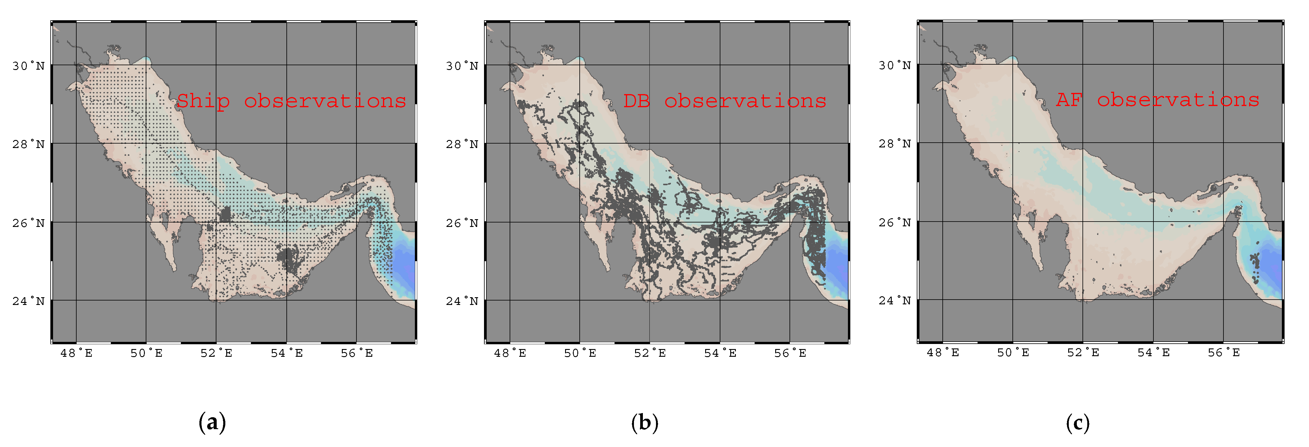
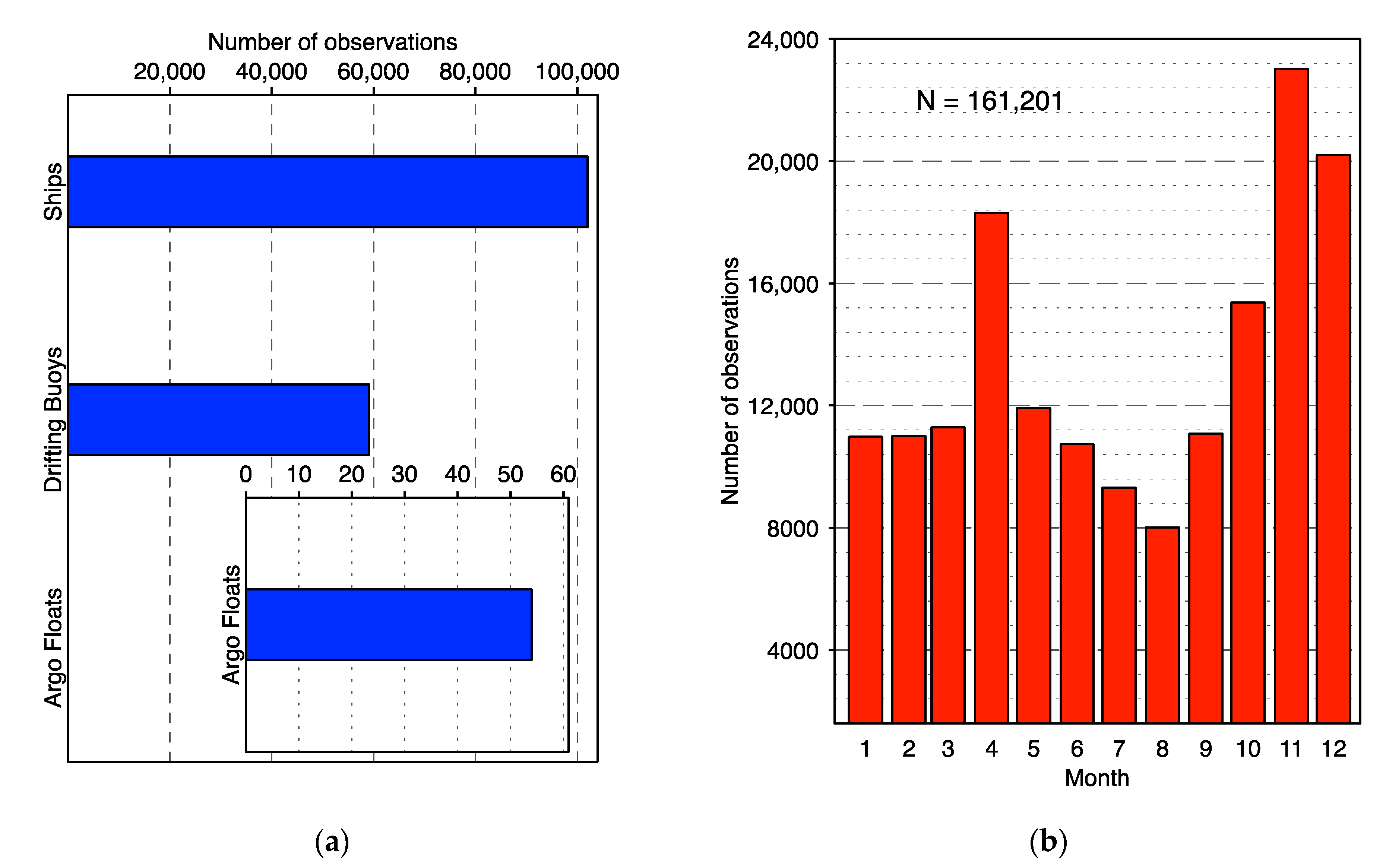
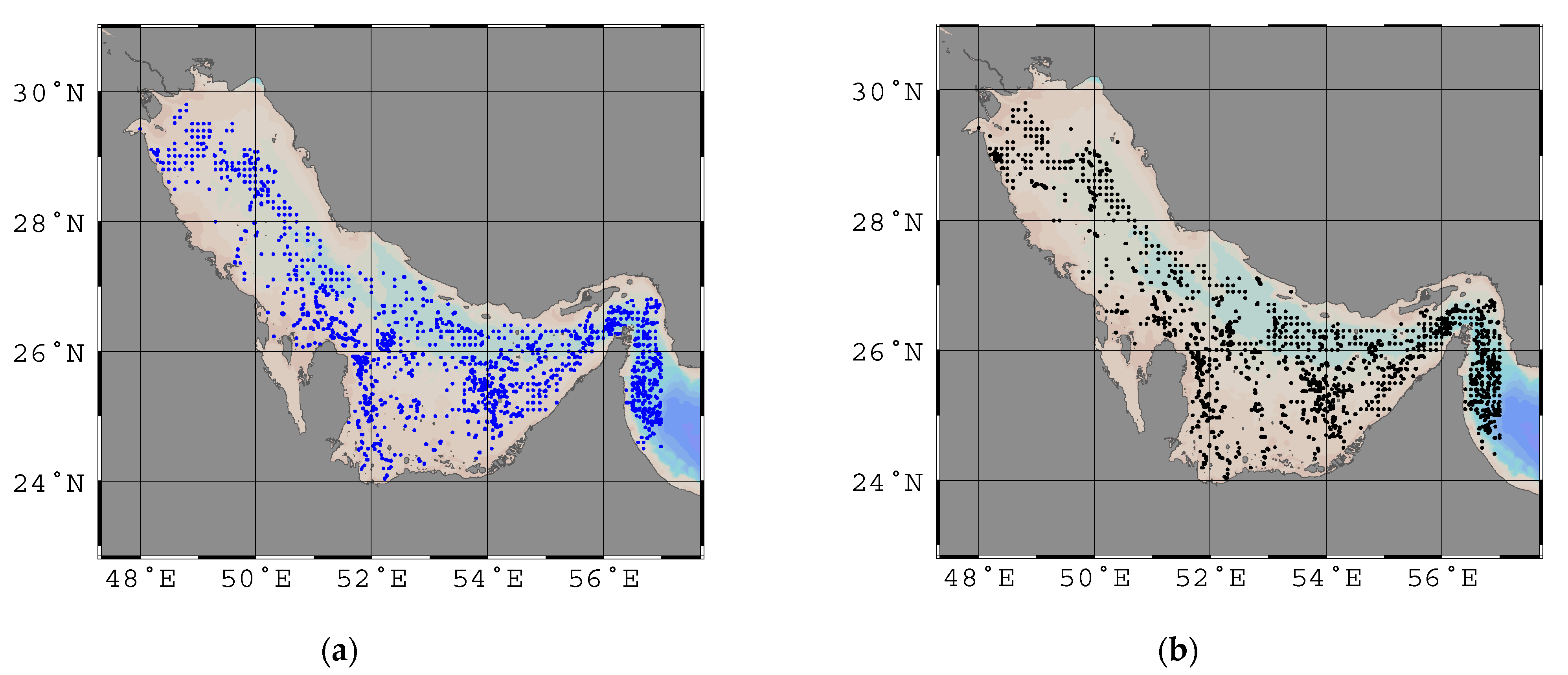
3.2. In Situ Observations
4. Methods of Comparison
4.1. Match-Up Protocol
4.2. Direct Comparison
4.3. Extended Triple Collocation
5. Results and Discussion
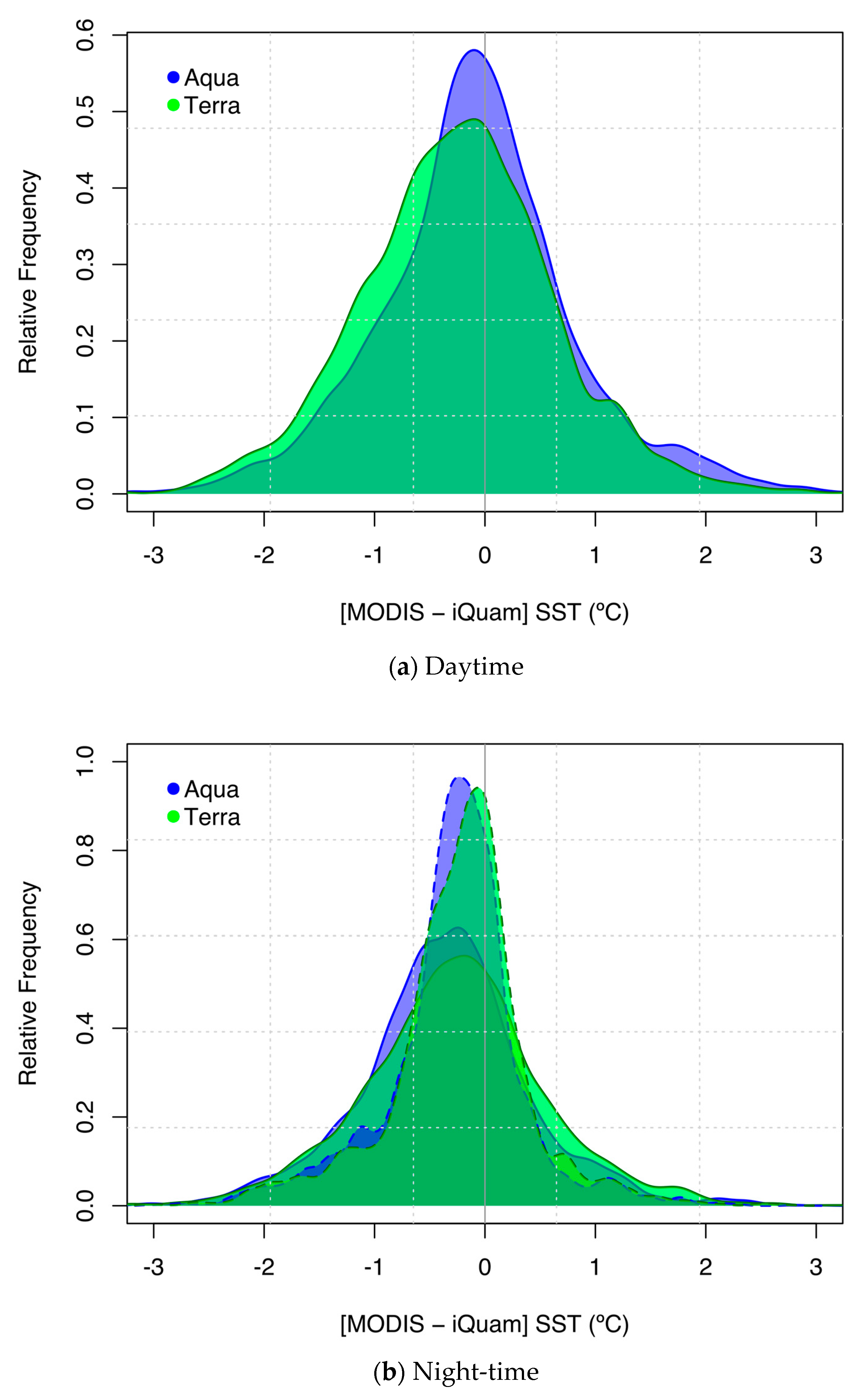
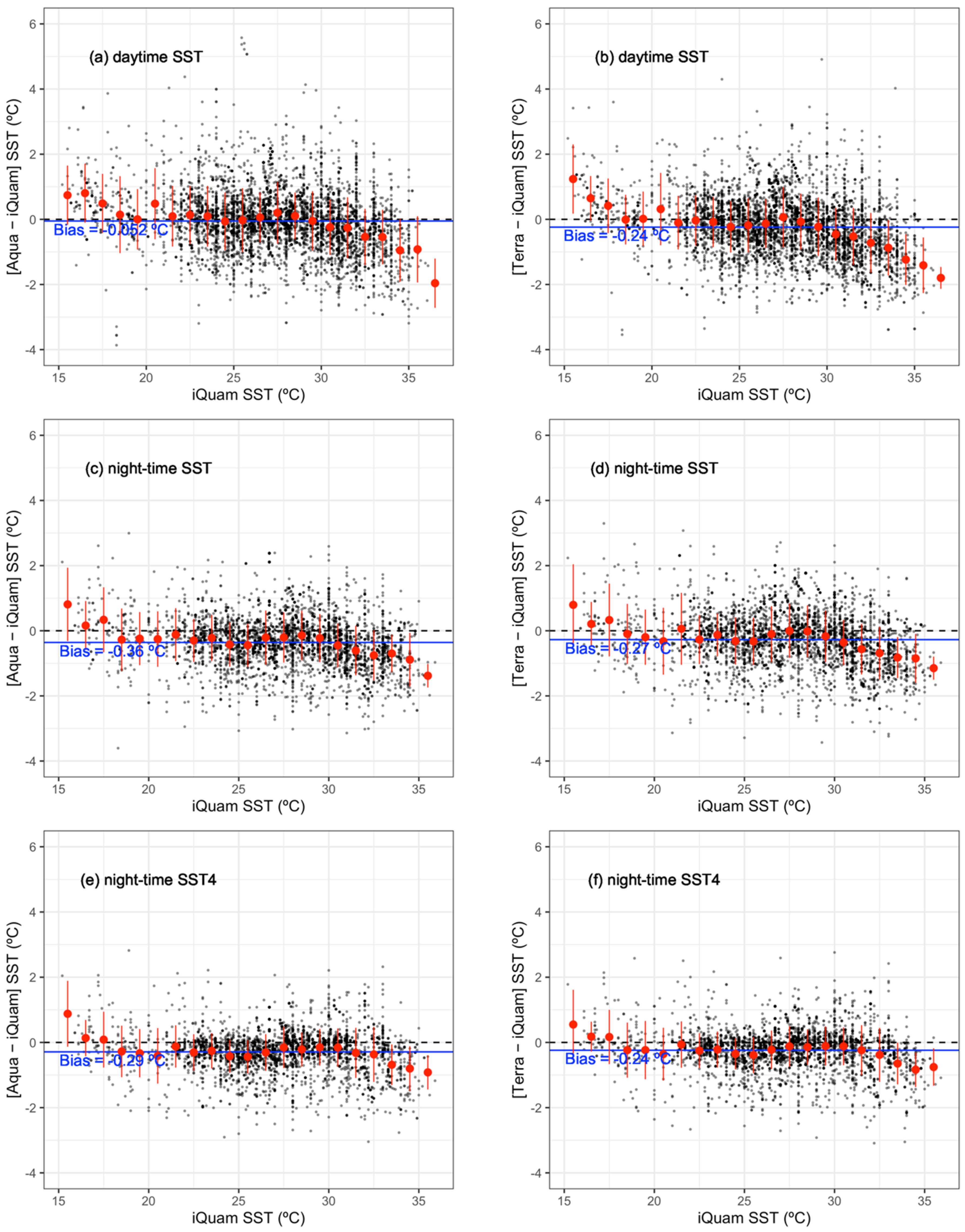
5.1. Systematic Errors
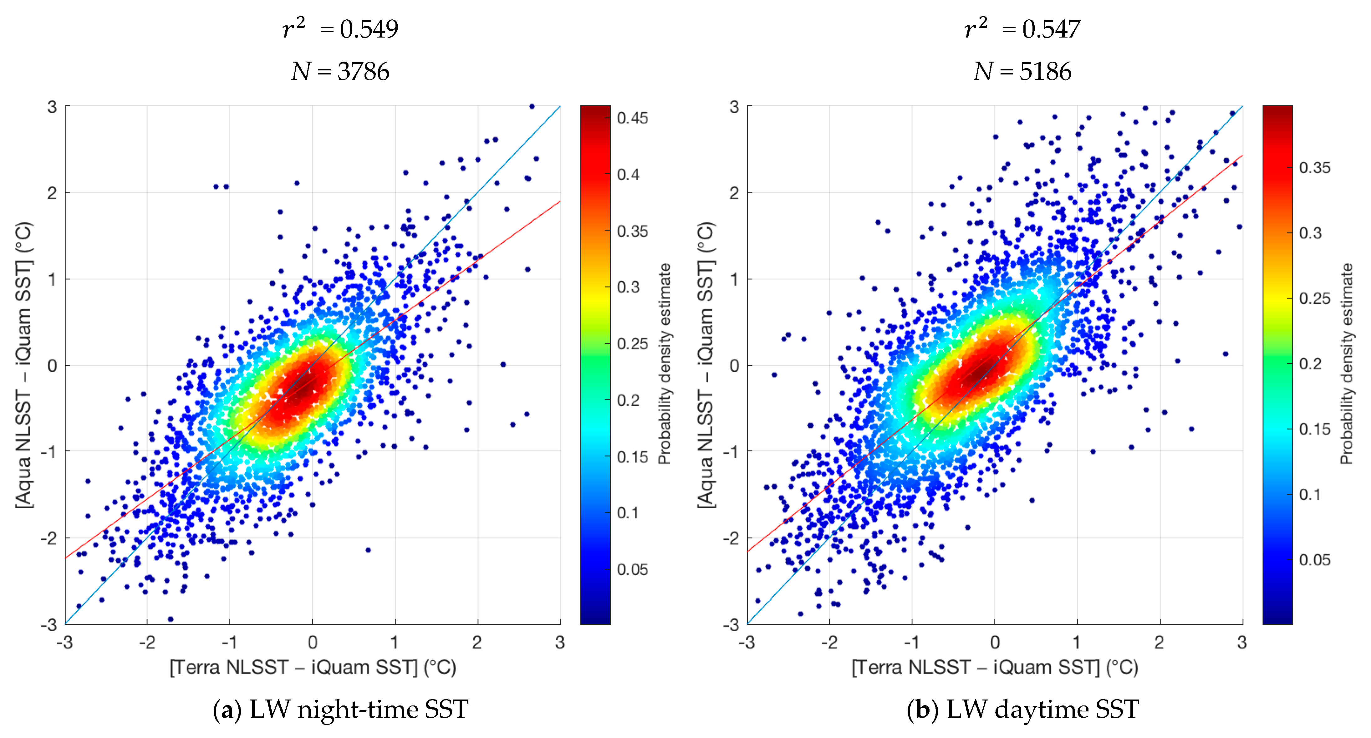
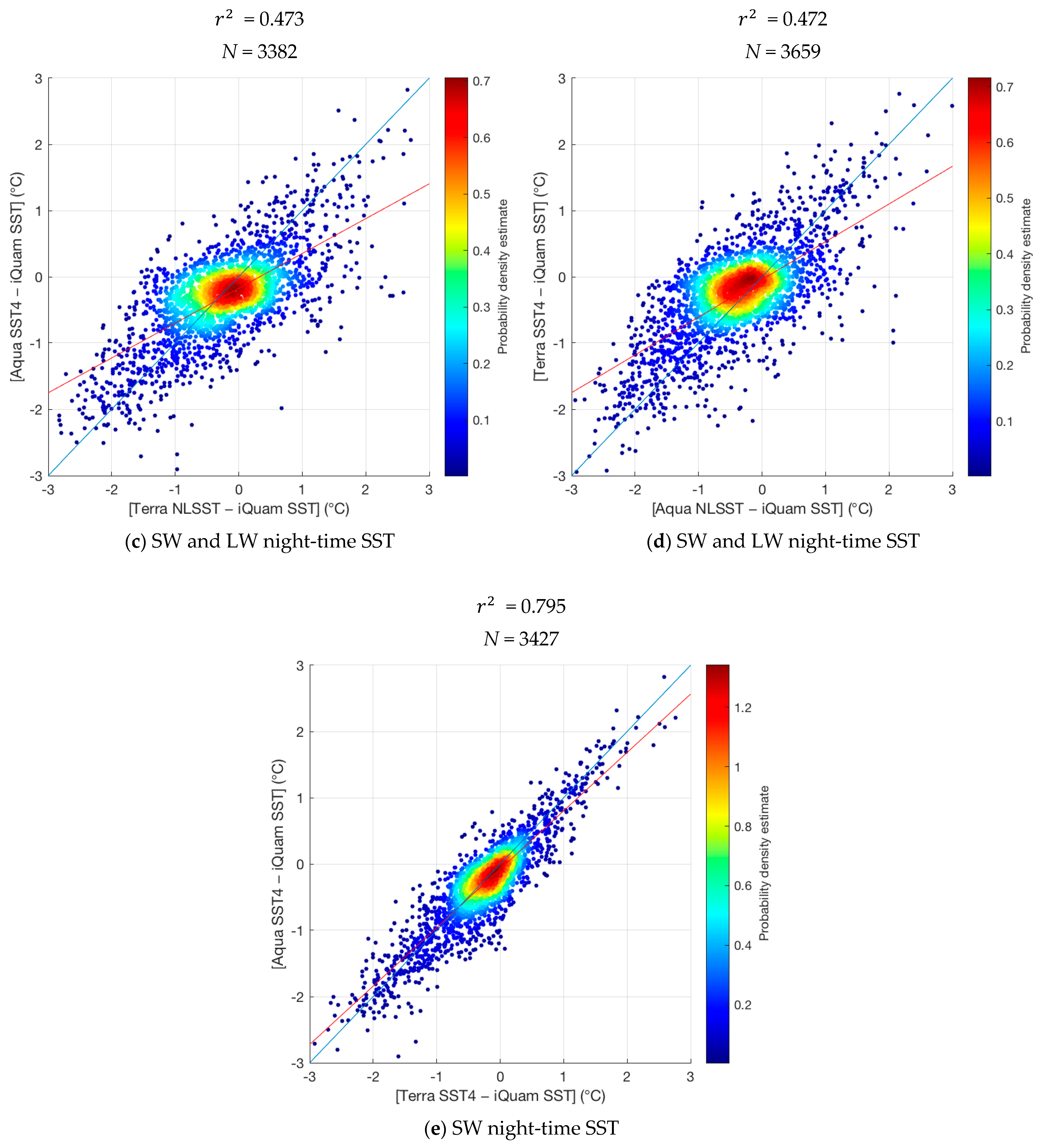
5.2. Data Independence
5.3. Direct Comparison versus Triple Collocation
6. Conclusions
Author Contributions
Funding
Institutional Review Board Statement
Informed Consent Statement
Data Availability Statement
Conflicts of Interest
References
- Fingas, M. Remote Sensing for Marine Management. In World Seas: An Environmental Evaluation; Sheppard, C., Ed.; Academic Press: Cambridge, MA, USA, 2019; pp. 103–119. ISBN 978-0-12-805052-1. [Google Scholar]
- Takahashi, T.; Sutherland, S.C.; Sweeney, C.; Poisson, A.; Metzl, N.; Tilbrook, B.; Bates, N.; Wanninkhof, R.; Feely, R.A.; Sabine, C.; et al. Global sea–air CO2 flux based on climatological surface ocean pCO2, and seasonal biological and temperature effects. Deep Sea Res. Part II Top. Stud. Oceanogr. 2002, 49, 1601–1622. [Google Scholar] [CrossRef]
- Stemmler, I.; Lammel, G. Air–sea exchange of semivolatile organic compounds—Wind and/or sea surface temperature control of volatilisation studied using a coupled general circulation model. J. Mar. Syst. 2011, 85, 11–18. [Google Scholar] [CrossRef]
- Yu, L. Sea surface exchanges of momentum, heat, and freshwater determined by satellite remote sensing. In Encyclopedia of Ocean Sciences; Elsevier: Amsterdam, The Netherlands, 2019; pp. 15–23. [Google Scholar]
- Song, Q.; Chelton, D.B.; Esbensen, S.K.; Thum, N.; O’Neill, L.W. Coupling between sea surface temperature and low-level winds in mesoscale numerical models. J. Clim. 2009, 22, 146–164. [Google Scholar] [CrossRef]
- Chelton, D.B.; Wentz, F.J. Global microwave satellite observations of sea surface temperature for numerical weather prediction and climate research. Bull. Am. Meteorol. Soc. 2005, 86, 1097–1116. [Google Scholar] [CrossRef] [Green Version]
- Maloney, E.D.; Chelton, D.B. An Assessment of the sea surface temperature influence on surface wind stress in numerical weather prediction and climate models. J. Clim. 2006, 19, 2743–2762. [Google Scholar] [CrossRef] [Green Version]
- Minnett, P.J.; Barton, I.J. Remote Sensing of the Earth’s Surface Temperature. In Radiometric Temperature Measurements: II. Applications; Zhang, Z., Tsai, B., Machin, G., Eds.; Academic Press: Cambridge, MA, USA, 2010; Volume 43, pp. 333–391. ISBN 1079-4042. [Google Scholar]
- Brown, O.B.; Minnett, P.J. MODIS infrared sea surface temperature algorithm theoretical basis document, version 2.0. Univ. Miami 1999, 31, 098-33. [Google Scholar]
- Kilpatrick, K.A.; Podestá, G.; Walsh, S.; Williams, E.; Halliwell, V.; Szczodrak, M.; Brown, O.B.; Minnett, P.J.; Evans, R. A decade of sea surface temperature from MODIS. Remote Sens. Environ. 2015, 165, 27–41. [Google Scholar] [CrossRef]
- Koner, P.K. Enhancing information content in the satellite-derived daytime infrared sea surface temperature dataset using a transformative approach. Front. Mar. Sci. 2020, 7, 1–16. [Google Scholar] [CrossRef]
- Koner, P.K. Daytime sea surface temperature retrieval incorporating mid-wave imager measurements: Algorithm development and validation. IEEE Trans. Geosci. Remote Sens. 2020, 59, 1–12. [Google Scholar] [CrossRef]
- Hosoda, K.; Qin, H. Algorithm for estimating sea surface temperatures based on Aqua/MODIS global ocean data. 1. Development and validation of the algorithm. J. Oceanogr. 2011, 67, 135–145. [Google Scholar] [CrossRef]
- Hosoda, K.; Murakami, H.; Sakaida, F.; Kawamura, H. Algorithm and validation of sea surface temperature observation using MODIS sensors aboard terra and aqua in the western North Pacific. J. Oceanogr. 2007, 63, 267–280. [Google Scholar] [CrossRef]
- Barnes, B.B.; Hu, C. A Hybrid Cloud Detection Algorithm to Improve MODIS Sea Surface Temperature Data Quality and Coverage Over the Eastern Gulf of Mexico. IEEE Trans. Geosci. Remote Sens. 2013, 51, 3273–3285. [Google Scholar] [CrossRef]
- Wang, J.; Deng, Z. Development of MODIS data-based algorithm for retrieving sea surface temperature in coastal waters. Environ. Monit. Assess. 2017, 189, 286. [Google Scholar] [CrossRef] [PubMed]
- Robinson, I.S. Measuring the Oceans from Space; Praxis Publishing Ltd.: Chichester, UK, 2004. [Google Scholar]
- Wentz, F.J. Satellite Measurements of sea surface temperature through clouds. Science 2000, 288, 847–850. [Google Scholar] [CrossRef] [PubMed] [Green Version]
- Schneider, P.; Healey, N.; Hulley, G.; Hook, S. Lake Surface Temperature. In Taking the Temperature of the Earth - Steps Towards Integrated Understanding of Variability and Change; Hulley, G., Ghent, D., Eds.; Elsevier: Amsterdam, The Netherlands, 2019; pp. 129–150. ISBN 978-0-12-814458-9. [Google Scholar]
- Wu, X.; Xiao, Q.; Wen, J.; You, D. Direct comparison and triple collocation: Which is more reliable in the validation of coarse-scale satellite surface albedo products. J. Geophys. Res. Atmos. 2019, 124, 5198–5213. [Google Scholar] [CrossRef]
- Glover, D.M.; Jenkins, W.J.; Doney, S.C. Modeling Methods for Marine Science; Cambridge University Press: Cambridge, UK, 2011. [Google Scholar]
- Stoffelen, A. Toward the true near-surface wind speed: Error modeling and calibration using triple collocation. J. Geophys. Res. Ocean. 1998, 103, 7755–7766. [Google Scholar] [CrossRef]
- Gruber, A.; Su, C.H.; Zwieback, S.; Crow, W.; Dorigo, W.; Wagner, W. Recent advances in (soil moisture) triple collocation analysis. Int. J. Appl. Earth Obs. Geoinf. 2016, 45, 200–211. [Google Scholar] [CrossRef]
- Saha, K.; Dash, P.; Zhao, X.; Zhang, H. Error estimation of pathfinder version 5.3 level-3C SST using extended triple collocation analysis. Remote Sens. 2020, 12, 590. [Google Scholar] [CrossRef] [Green Version]
- O’Carroll, A.G.; Eyre, J.R.; Saunders, R.W. Three-way error analysis between AATSR, AMSR-E, and in situ sea surface temperature observations. J. Atmos. Ocean. Technol. 2008, 25, 1197–1207. [Google Scholar] [CrossRef] [Green Version]
- O’Carroll, A.G.; August, T.; Le Borgne, P.; Marsouin, A. The accuracy of SST retrievals from Metop-A IASI and AVHRR using the EUMETSAT OSI-SAF matchup dataset. Remote Sens. Environ. 2012, 126, 184–194. [Google Scholar] [CrossRef]
- Gentemann, C.L. Three way validation of MODIS and AMSR-E sea surface temperatures. J. Geophys. Res. Ocean. 2014, 119, 2583–2598. [Google Scholar] [CrossRef]
- Blackmore, T.; O’Carroll, A.; Fennig, K.; Saunders, R. Correction of AVHRR Pathfinder SST data for volcanic aerosol effects using ATSR SSTs and TOMS aerosol optical depth. Remote Sens. Environ. 2012, 116, 107–117. [Google Scholar] [CrossRef]
- Tsamalis, C.; Saunders, R. Quality Assessment of sea surface temperature from ATSRs of the climate change initiative (phase 1). Remote Sens. 2018, 10, 497. [Google Scholar] [CrossRef] [Green Version]
- Wirasatriya, A.; Hosoda, K.; Setiawan, J.D.; Susanto, R.D. Variability of diurnal sea surface temperature during short term and high SST event in the western equatorial pacific as revealed by satellite data. Remote Sens. 2020, 12, 3230. [Google Scholar] [CrossRef]
- Hoareau, N.; Portabella, M.; Lin, W.; Ballabrera-Poy, J.; Turiel, A. Error characterization of sea surface salinity products using triple collocation analysis. IEEE Trans. Geosci. Remote Sens. 2018, 56, 5160–5168. [Google Scholar] [CrossRef]
- Miyaoka, K.; Gruber, A.; Ticconi, F.; Hahn, S.; Wagner, W.; Figa-Saldaña, J.; Anderson, C. Triple collocation analysis of soil moisture from metop-a ASCAT and SMOS against JRA-55 and ERA-interim. IEEE J. Sel. Top. Appl. Earth Obs. Remote Sens. 2017, 10, 2274–2284. [Google Scholar] [CrossRef]
- Gruber, A.; Dorigo, W.A.; Crow, W.; Wagner, W. Triple collocation-based merging of satellite soil moisture retrievals. IEEE Trans. Geosci. Remote Sens. 2017, 55, 6780–6792. [Google Scholar] [CrossRef]
- Su, C.H.; Ryu, D.; Crow, W.T.; Western, A.W. Beyond triple collocation: Applications to soil moisture monitoring. J. Geophys. Res. Atmos. 2014, 119, 6419–6439. [Google Scholar] [CrossRef]
- Zhu, H.; Zhang, Z.; Lv, A. Evaluation of satellite-derived soil moisture in Qinghai province based on triple collocation. Water 2020, 12, 1292. [Google Scholar] [CrossRef]
- Lyu, F.; Tang, G.; Behrangi, A.; Wang, T.; Tan, X.; Ma, Z.; Xiong, W. Precipitation Merging Based on the Triple Collocation Method Across Mainland China. IEEE Trans. Geosci. Remote Sens. 2021, 59, 3161–3176. [Google Scholar] [CrossRef]
- Hao, Y.; Cui, T.; Singh, V.P.; Zhang, J.; Yu, R.; Zhang, Z. Validation of MODIS sea surface temperature product in the coastal waters of the Yellow Sea. IEEE J. Sel. Top. Appl. Earth Obs. Remote Sens. 2017, 10, 1667–1680. [Google Scholar] [CrossRef]
- Castro, S.L.; Wick, G.A.; Emery, W.J. Evaluation of the relative performance of sea surface temperature measurements from different types of drifting and moored buoys using satellite-derived reference products. J. Geophys. Res. Ocean. 2012, 117, 1–19. [Google Scholar] [CrossRef]
- Guan, L.; Kawamura, H. SST availabilities of satellite infrared and microwave measurements. J. Oceanogr. 2003, 59, 201–209. [Google Scholar] [CrossRef]
- Ghanea, M.; Moradi, M.; Kabiri, K.; Mehdinia, A. Investigation and validation of MODIS SST in the northern Persian Gulf. Adv. Sp. Res. 2016, 57, 127–136. [Google Scholar] [CrossRef]
- Lee, M.A.; Tzeng, M.T.; Hosoda, K.; Sakaida, F.; Kawamura, H.; Shieh, W.J.; Yang, Y.; Chang, Y. Validation of JAXA/MODIS sea surface temperature in water around Taiwan using the terra and aqua satellites. Terr. Atmos. Ocean. Sci. 2010, 21, 727. [Google Scholar] [CrossRef] [Green Version]
- Qin, H.; Chen, G.; Wang, W.; Wang, D.; Zeng, L. Validation and application of MODIS-derived SST in the South China Sea. Int. J. Remote Sens. 2014, 35, 4315–4328. [Google Scholar] [CrossRef]
- Hosoda, K.; Murakami, H. Validation of near-real-time sea surface temperature from MODIS in the ocean around Japan. In Proceedings of the 2005 IEEE International Geoscience and Remote Sensing Symposium, Seoul, Korea, 29 July 2005; Volume 4, pp. 2614–2616. [Google Scholar]
- Høyer, J.L.; Karagali, I.; Dybkjær, G.; Tonboe, R. Multi sensor validation and error characteristics of Arctic satellite sea surface temperature observations. Remote Sens. Environ. 2012, 121, 335–346. [Google Scholar] [CrossRef]
- Knievel, J.C.; Rife, D.L.; Grim, J.A.; Hahmann, A.N.; Hacker, J.P.; Ge, M.; Fisher, H.H. A Simple Technique for creating regional composites of sea surface temperature from MODIS for use in operational mesoscale NWP. J. Appl. Meteorol. Climatol. 2010, 49, 2267–2284. [Google Scholar] [CrossRef] [Green Version]
- Pan, X.; Wong, G.T.F.; DeCarlo, T.M.; Tai, J.H.; Cohen, A.L. Validation of the remotely sensed nighttime sea surface temperature in the shallow waters at the Dongsha Atoll. Terr. Atmos. Ocean. Sci. 2017, 28, 517–524. [Google Scholar] [CrossRef] [Green Version]
- Durá, E.; Mendiguren, G.; Martín, M.P.; Acevedo-Dudley, M.J.; Bosch-Bolmar, M.; Fuentes, V.L.; Bordehore, C. Validación local de la temperatura superficial del mar del sensor MODIS en aguas someras del Mediterráneo occidental. Rev. Teledetección 2014, 41, 59–69. [Google Scholar] [CrossRef] [Green Version]
- Barton, I.; Pearce, A. Validation of GLI and other satellite-derived sea surface temperatures using data from the Rottnest Island ferry, Western Australia. J. Oceanogr. 2006, 62, 303–310. [Google Scholar] [CrossRef]
- Cervone, G. Combined remote-sensing, model, and in situ measurements of sea surface temperature as an aid to recreational navigation: Crossing the Gulf Stream. Int. J. Remote Sens. 2013, 34, 434–450. [Google Scholar] [CrossRef]
- Guo, P.; Bo, Y. Validation of AVHRR/MODIS/AMSR-E satellite SST products in the west Tropical Pacific. In Proceedings of the IGARSS 2008–2008 IEEE International Geoscience and Remote Sensing Symposium, Boston, MA, USA, 7–11 July 2008; Volume 4, pp. 942–945. [Google Scholar]
- Haines, S.L.; Jedlovec, G.J.; Lazarus, S.M. A MODIS sea surface temperature composite for regional applications. IEEE Trans. Geosci. Remote Sens. 2007, 45, 2919–2927. [Google Scholar] [CrossRef]
- Tyagi, G.; Babu, K.N.; Mathur, A.K.; Solanki, H.A. INSAT-3D and MODIS retrieved sea surface temperature validation and assessment over waters surrounding the Indian subcontinent. Int. J. Remote Sens. 2018, 39, 1575–1592. [Google Scholar] [CrossRef]
- Barton, I.J. Comparison of in situ and satellite-derived sea surface temperatures in the Gulf of Carpentaria. J. Atmos. Ocean. Technol. 2007, 24, 1773–1784. [Google Scholar] [CrossRef]
- Alsahli, M. Characterizing Surface Temperature and Clarity of Kuwait’s Seawaters Using Remotely Sensed Measurements and GIS Analyses. Ph.D. Thesis, University of Kansas, Lawrence, KS, USA, November 2009. Available online: https://kuscholarworks.ku.edu/handle/1808/5969 (accessed on 28 February 2020).
- Kozlov, I.; Dailidienė, I.; Korosov, A.; Klemas, V.; Mingėlaitė, T. MODIS-based sea surface temperature of the Baltic Sea Curonian Lagoon. J. Mar. Syst. 2014, 129, 157–165. [Google Scholar] [CrossRef]
- Marcello, J.; Eugenio, F.; Hernandez, A. Validation of MODIS and AVHRR/3 sea surface temperature retrieval algorithms. In Proceedings of the 2004 IEEE International Geoscience and Remote Sensing Symposium, Anchorage, AK, USA, 20–24 September 2004; Volume 2, pp. 839–842. [Google Scholar]
- Ahmadabadi, A.; Fathnia, A.; Karimi Ahmadabad, M.; Farajzadeh, M. The accuracy of SST retrievals from NOAA-AVHRR in the Persian Gulf. J. Appl. Sci. 2009, 9, 1378–1382. [Google Scholar] [CrossRef]
- Al-Rashidi, T.B.; El-Gamily, H.I.; Amos, C.L.; Rakha, K.A. Sea surface temperature trends in Kuwait Bay, Arabian Gulf. Nat. Hazards 2009, 50, 73–82. [Google Scholar] [CrossRef]
- Vaughan, G.; Al-Mansoori, N.; Burt, J. The Arabian Gulf. In World Seas: An Environmental Evaluation; Sheppard, C., Ed.; Academic Press: Cambridge, MA, USA, 2019; pp. 1–23. ISBN 978-0-08-100853-9. [Google Scholar]
- Michael Reynolds, R. Physical oceanography of the Gulf, Strait of Hormuz, and the Gulf of Oman—Results from the Mt Mitchell expedition. Mar. Pollut. Bull. 1993, 27, 35–59. [Google Scholar] [CrossRef]
- ROPME (Regional Organization for the Protection of the Marine Environment). State of the Marine Environment Report; Regional Organization for the Protection of the Marine Environment: Kuwait City, Kuwait, 2013; Available online: http://www.ropme.org/Uploads/Events/EBM/03-SOMER_2013.pdf (accessed on 13 April 2021).
- Purser, B.H.; Seibold, E. Holocene carbonate sedimentation and diagenesis in a shallow epicontinental sea. In The Persian Gulf; Purser, B.H., Ed.; Springer: Heidelberg, Germany, 1973. [Google Scholar]
- Walters, K.; Sjoberg, W. The Persian Gulf Region, A Climatological Study. 1988. Available online: https://apps.dtic.mil/dtic/tr/fulltext/u2/a222654.pdf (accessed on 13 April 2021).
- Boyer, T.P.; Antonov, J.I.; Baranova, O.K.; Coleman, C.; Garcia, H.E.; Grodsky, A.; Johnson, D.R.; Locarnini, R.A.; Mishonov, A.V.; O’Brien, T.D.; et al. World Ocean Database 2013; NOAA Atlas NESDIS 72; Levitus, S., Technical, A.M., Eds.; NOAA: Silver Spring, MD, USA, 2013.
- Minnett, P.J.; Alvera-Azcárate, A.; Chin, T.M.; Corlett, G.K.; Gentemann, C.L.; Karagali, I.; Li, X.; Marsouin, A.; Marullo, S.; Maturi, E.; et al. Half a century of satellite remote sensing of sea-surface temperature. Remote Sens. Environ. 2019, 233, 111366. [Google Scholar] [CrossRef]
- Shutler, J.D.; Smyth, T.J.; Land, P.E.; Groom, S.B. A near-real time automatic MODIS data processing system. Int. J. Remote Sens. 2005, 26, 1049–1055. [Google Scholar] [CrossRef]
- Walton, C.C.; Pichel, W.G.; Sapper, J.F.; May, D.A. The development and operational application of nonlinear algorithms for the measurement of sea surface temperatures with the NOAA polar-orbiting environmental satellites. J. Geophys. Res. Ocean. 1998, 103, 27999–28012. [Google Scholar] [CrossRef]
- Reynolds, R.W.; Rayner, N.A.; Smith, T.M.; Stokes, D.C.; Wang, W. An improved in situ and satellite SST analysis for climate. J. Clim. 2002, 15, 1609–1625. [Google Scholar] [CrossRef]
- Reynolds, R.W.; Smith, T.M.; Liu, C.; Chelton, D.B.; Casey, K.S.; Schlax, M.G. Daily high-resolution-blended analyses for sea surface temperature. J. Clim. 2007, 20, 5473–5496. [Google Scholar] [CrossRef]
- Kilpatrick, K.A.; Podestá, G.; Williams, E.; Walsh, S.; Minnett, P.J. Alternating decision trees for cloud masking in MODIS and VIIRS NASA sea surface temperature products. J. Atmos. Ocean. Technol. 2019, 36, 387–407. [Google Scholar] [CrossRef]
- Savtchenko, A.; Ouzounov, D.; Ahmad, S.; Acker, J.; Leptoukh, G.; Koziana, J.; Nickless, D. Terra and aqua MODIS products available from NASA GES DAAC. Adv. Sp. Res. 2004, 34, 710–714. [Google Scholar] [CrossRef]
- Donlon, C.J.; Minnett, P.J.; Gentemann, C.; Nightingale, T.J.; Barton, I.J.; Ward, B.; Murray, M.J. Toward improved validation of satellite sea surface skin temperature measurements for climate research. J. Clim. 2002, 15, 353–369. [Google Scholar] [CrossRef] [Green Version]
- Schluessel, P.; Emery, W.J.; Grassl, H.; Mammen, T. On the bulk-skin temperature difference and its impact on satellite remote sensing of sea surface temperature. J. Geophys. Res. Ocean. 1990, 95, 13341–13356. [Google Scholar] [CrossRef]
- Xu, F.; Ignatov, A. In situ SST quality monitor (iQuam). J. Atmos. Ocean. Technol. 2014, 31, 164–180. [Google Scholar] [CrossRef]
- Schlitzer, R. Ocean Data View 2018. Available online: https://odv.awi.de (accessed on 13 April 2021).
- Xu, F.; Ignatov, A. Evaluation of in situ sea surface temperatures for use in the calibration and validation of satellite retrievals. J. Geophys. Res. Ocean. 2010, 115, 1–18. [Google Scholar] [CrossRef]
- Xu, F.; Ignatov, A. Error characterization in iQuam SSTs using triple collocations with satellite measurements. Geophys. Res. Lett. 2016, 43. [Google Scholar] [CrossRef]
- Lafon, V.; Martins, A.; Figueiredo, M.; Melo Rodrigues, M.A.; Bashmachnikov, I.; Mendonça, A.; Macedo, L.; Goulart, N. Sea surface temperature distribution in the Azores region. Part I: AVHRR imagery and in situ data processing. Arquipélago Life Mar. Sci. 2004, 21, 1–18. [Google Scholar]
- Delgado, A.L.; Jamet, C.; Loisel, H.; Vantrepotte, V.; Perillo, G.M.E.; Piccolo, M.C. Evaluation of the MODIS-aqua sea-surface Temperature product in the inner and mid-shelves of southwest Buenos Aires Province, Argentina. Int. J. Remote Sens. 2014, 35, 306–320. [Google Scholar] [CrossRef]
- Legendre, P.; Legendre, L. Number 24 in Developments in Environmental Modelling, 3rd ed.; Elsevier: Amsterdam, The Netherlands, 2012. [Google Scholar]
- Legendre, P. Model II Regression User’s Guide, R Edition. 2018. Available online: https://cran.r-project.org/web/packages/lmodel2/vignettes/mod2user.pdf (accessed on 13 April 2021).
- Willmott, C.J. Advantages of the mean absolute error (MAE) over the root mean square error (RMSE) in assessing average model performance. Clim. Res. 2005, 30, 79–82. [Google Scholar] [CrossRef]
- Mélin, F.; Franz, B.A. Assessment of satellite ocean colour radiometry and derived geophysical products. In Optical Radiometry for Ocean Climate Measurements; Zibordi, G., Donlon, C.J., Parr, A.C., Eds.; Academic Press: Cambridge, MA, USA, 2014; Volume 47, pp. 609–638. [Google Scholar]
- McColl, K.A.; Vogelzang, J.; Konings, A.G.; Entekhabi, D.; Piles, M.; Stoffelen, A. Extended triple collocation: Estimating errors and correlation coefficients with respect to an unknown target. Geophys. Res. Lett. 2014, 41, 6229–6236. [Google Scholar] [CrossRef] [Green Version]
- Embury, O.; Merchant, C.J.; Corlett, G.K. A reprocessing for climate of sea surface temperature from the along-track scanning radiometers: Initial validation, accounting for skin and diurnal variability effects. Remote Sens. Environ. 2012, 116, 62–78. [Google Scholar] [CrossRef] [Green Version]
- Zhu, Y.; Bo, Y.; Zhang, J.; Wang, Y. Fusion of multisensor SSTs based on the spatiotemporal hierarchical Bayesian model. J. Atmos. Ocean. Technol. 2017, 35, 91–109. [Google Scholar] [CrossRef]
- Dong, S.; Gille, S.T.; Sprintall, J.; Gentemann, C. Validation of the advanced microwave scanning radiometer for the earth observing system (AMSR-E) sea surface temperature in the Southern Ocean. J. Geophys. Res. 2006, 111, C04002. [Google Scholar] [CrossRef]
- Yakubu, C.I.; Ayer, J.; Laari, P.B.; Amponsah, T.Y.; Hancock, C.M. A mutual assessment of the uncertainties of digital elevation models using the triple collocation technique. Int. J. Remote Sens. 2019, 40, 5301–5314. [Google Scholar] [CrossRef]
- Alemohammad, S.H.; McColl, K.A.; Konings, A.G.; Entekhabi, D.; Stoffelen, A. Characterization of precipitation product errors across the United States using multiplicative triple collocation. Hydrol. Earth Syst. Sci. 2015, 19. [Google Scholar] [CrossRef] [Green Version]
- Wu, X.; Lu, G.; Wu, Z.; He, H.; Scanlon, T.; Dorigo, W. Triple collocation-based assessment of satellite soil moisture products with in situ measurements in china: Understanding the error sources. Remote Sens. 2020, 12, 2275. [Google Scholar] [CrossRef]
- Ribal, A.; Young, I.R. Global calibration and error estimation of altimeter, scatterometer, and radiometer wind speed using triple collocation. Remote Sens. 2020, 12, 1997. [Google Scholar] [CrossRef]


| Abbreviation | Full Name |
|---|---|
| AVHRR | Advanced Very High-Resolution Radiometer |
| DSST | Daytime sea surface temperature |
| EPDF | Empirical probability density function |
| ETC | Extended triple collocation |
| GEBCO | General Bathymetric Chart of the Oceans |
| iQuam | in situ SST Quality Monitor |
| IR | Infrared |
| LWIR | Long-wave infrared |
| MODIS | Moderate Resolution Imaging Spectroradiometer |
| MW | Microwave |
| MWIR | Mid-wave infrared |
| NLSST | Nonlinear sea surface temperature |
| NOAA | National Oceanic and Atmospheric Administration |
| NRT | Near real-time |
| NSST | Night-time sea surface temperature |
| PDE | Probability density estimate |
| SeaDAS | SeaWiFS Data Analysis System |
| TCA | Tiple collocation analysis |
| SST | Sea surface temperature |
| SST4 | short-wave sea surface temperature |
| WOD | World ocean database |
| XBT | Expendable bathythermograph |
| Reference | Study Area | Satellite | Number of Matches | Validation Metrics | RMSE (in °C Unless Otherwise Stated) | Time |
|---|---|---|---|---|---|---|
| [37] | Yellow Sea Coasts | Aqua | 164 | R2 = 0.987 | 0.85 | Daytime |
| Terra | 154 | R2 = 0.989 | 0.83 | Daytime | ||
| [40] | Northern Arabian Gulf | Aqua | 63 | R2 = 0.9898 | 0.53 | Daytime |
| Terra | 78 | R2 = 0.9932 | 0.44 | Daytime | ||
| [41] | Taiwan Waters | Aqua | 151 | Bias (°C) = 0.44 Bias (°C) = −0.01 | 0.88 0.71 | Daytime |
| Night-time | ||||||
| Terra | 139 | Bias (°C) = −0.41 Bias (°C) = −0.13 | 0.71 0.60 | Daytime | ||
| Night-time | ||||||
| [42] | Southern China Sea | Both satellites | 3605 | Bias (°C) = −0.22 (cruise), −0.16 (observation station) and −0.11 (WOD09) | – | Daytime |
| Bias (°C) = −0.32 (cruise), −0.57 (observation station) and −0.27 (WOD09) | – | Night-time | ||||
| [14] | NW Pacific | Aqua | 12,222 | Bias (°C) = −0.014 Bias (°C) = −0.141 | 0.70 0.65 | Daytime |
| Night-time | ||||||
| Terra | 12,525 | Bias (°C) = −0.041 Bias (°C) = −0.052 | 0.65 0.66 | Daytime | ||
| Night-time | ||||||
| [43] | Japan waters | Aqua | 3394 | Bias (K) = −0.17 Bias (K) = 0.19 | 0.61 K 0.46 K | Daytime |
| Night-time | ||||||
| Terra | 2597 | Bias (K) = −0.07 Bias (K) = 0.05 | 0.50 K 0.41 K | Daytime | ||
| Night-time | ||||||
| [44] | Arctic Ocean | Aqua | 210,273 | Bias (°C) = −0.73 | – | Night-time |
| Terra | 166,990 | Bias (°C) = −0.68 | – | Night-time | ||
| [45] | Florida Coasts | Both satellites | 36,020 | Bias (°C) = 0.05 Bias (°C) = −0.25 | 1.66 1.65 | Daytime |
| Night-time | ||||||
| [46] | Dongsha Atoll | Aqua | 466 | Bias (°C) = −0.43 | 0.73 | Night-time |
| [47] | Western Mediterranean Sea | Aqua | 29 | r2 = 0.96 | 1.00 | Daytime |
| 30 | r2 = 0.86 | 1.50 | Night-time | |||
| [48] | Rottnest Island in Western Australia | Terra | 866 | Bias (°C) = −0.32 | – | – |
| [49] | Gulf Stream region | Aqua | – | r = 0.94 | – | – |
| [50] | West Tropical Pacific | Aqua | – | Bias (°C) = −0.213 | 0.697 | – |
| [51] | Florida Peninsula waters | Aqua | – | r = 0.88 Bias (°C) = −0.09 r = 0.87 Bias (°C) = −0.29 | 0.68 | Daytime |
| 0.59 | Night-time | |||||
| [52] | Arabian Sea and Bay of Bengal | Aqua | 2895 | R2 = 0.76 Bias (°C) = 0.06 | 0.60 | – |
| Terra | 2875 | R2 = 0.75 Bias (°C) = −0.09 | 0.61 | – | ||
| [53] | Gulf of Carpentaria | Aqua | 24 | Bias (°C) = 0.05 | – | – |
| Terra | 23 | Bias (°C) = −0.15 | – | – | ||
| [54] | Kuwait’s seawaters | Aqua | 118 | r2 = 0.98 Median bias (°C) = 0.05 | 0.701 | Daytime |
| [55] | Baltic Sea Curonian Lagoon | Aqua | 13 | R2 = 0.78 Bias (°C) = 0.46 | 1.07 | Daytime |
| Terra | 18 | R2 = 0.84 Bias (°C) = 0.49 | 0.83 | Daytime | ||
| [56] | Canary Islands-Azores-Gibraltar area | Terra | 51 | Bias (°C) = −0.251 | 0.505 | Daytime & Night-time |
| Retrieval Time | Number of Matchups | [Aqua–Terra] SST (°C) | [Terra–iQuam] SST (°C) | [Aqua–iQuam] SST (°C) | |||
|---|---|---|---|---|---|---|---|
| Mean Bias | SD | Mean Bias | SD | Mean Bias | SD | ||
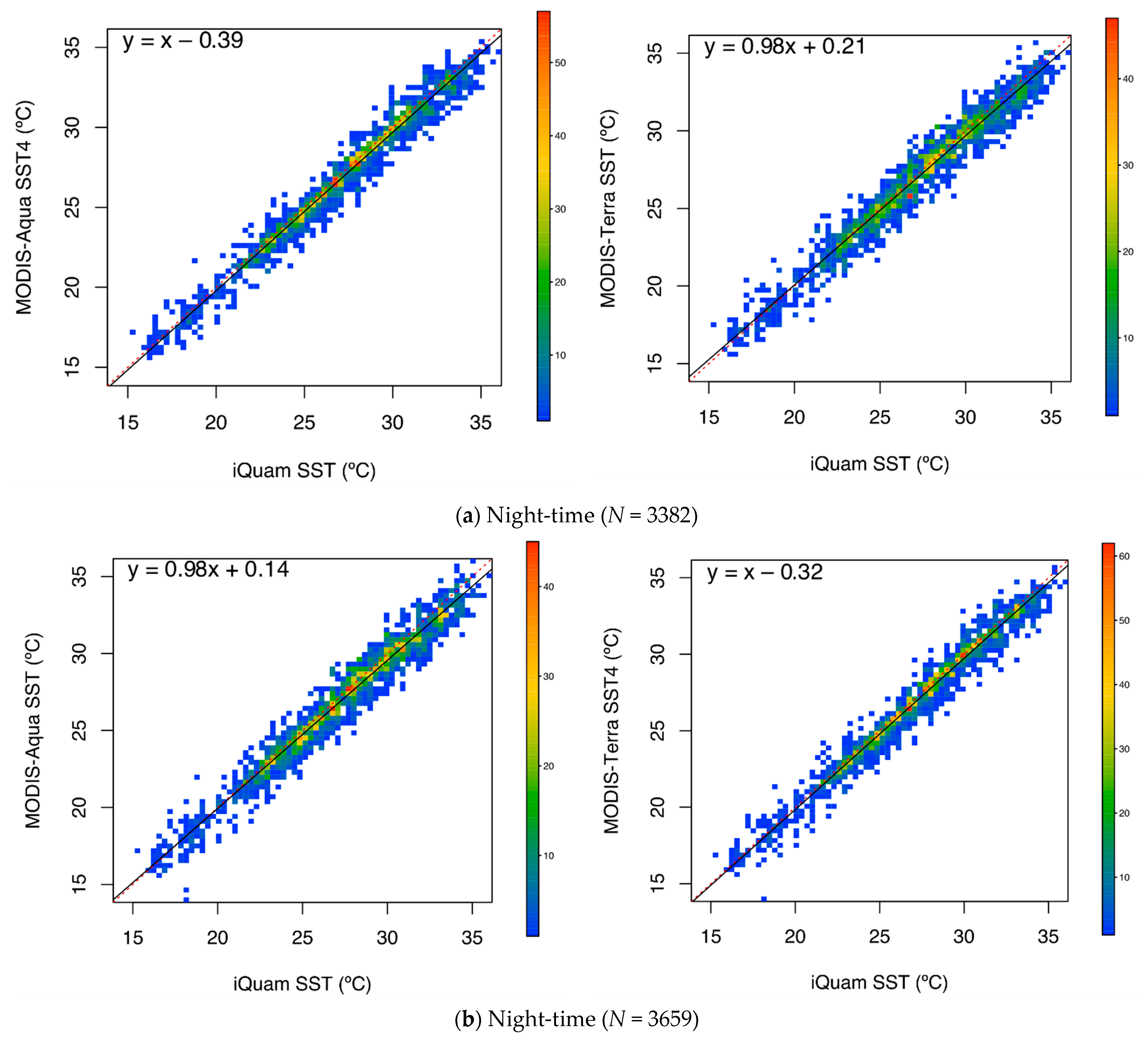
| Night-time | 3786 (3427) | −0.090 | 0.58 | −0.27 | 0.83 | −0.36 | 0.77 |
| (−0.050) | (0.30) | (−0.24) | (0.64) | (−0.29) | (0.63) | ||
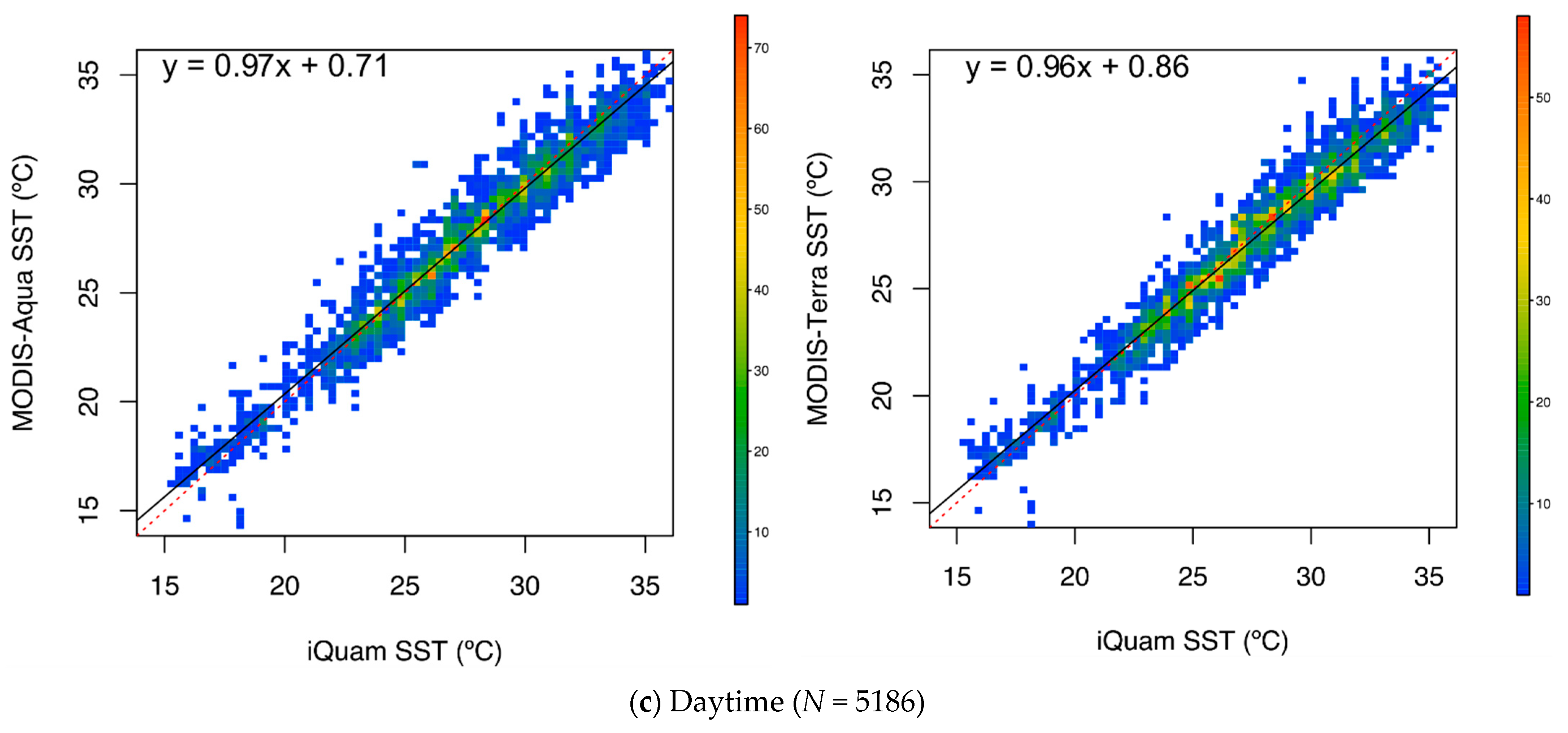
| Daytime | 5186 | 0.19 | 0.66 | −0.24 | 0.90 | −0.052 | 0.93 |
| Case | Retrieval Time | Data Set | Algorithm | ETC | Direct Comparison 1 | |||
|---|---|---|---|---|---|---|---|---|
| RMSE (°C) | RMSEub (°C) | |||||||
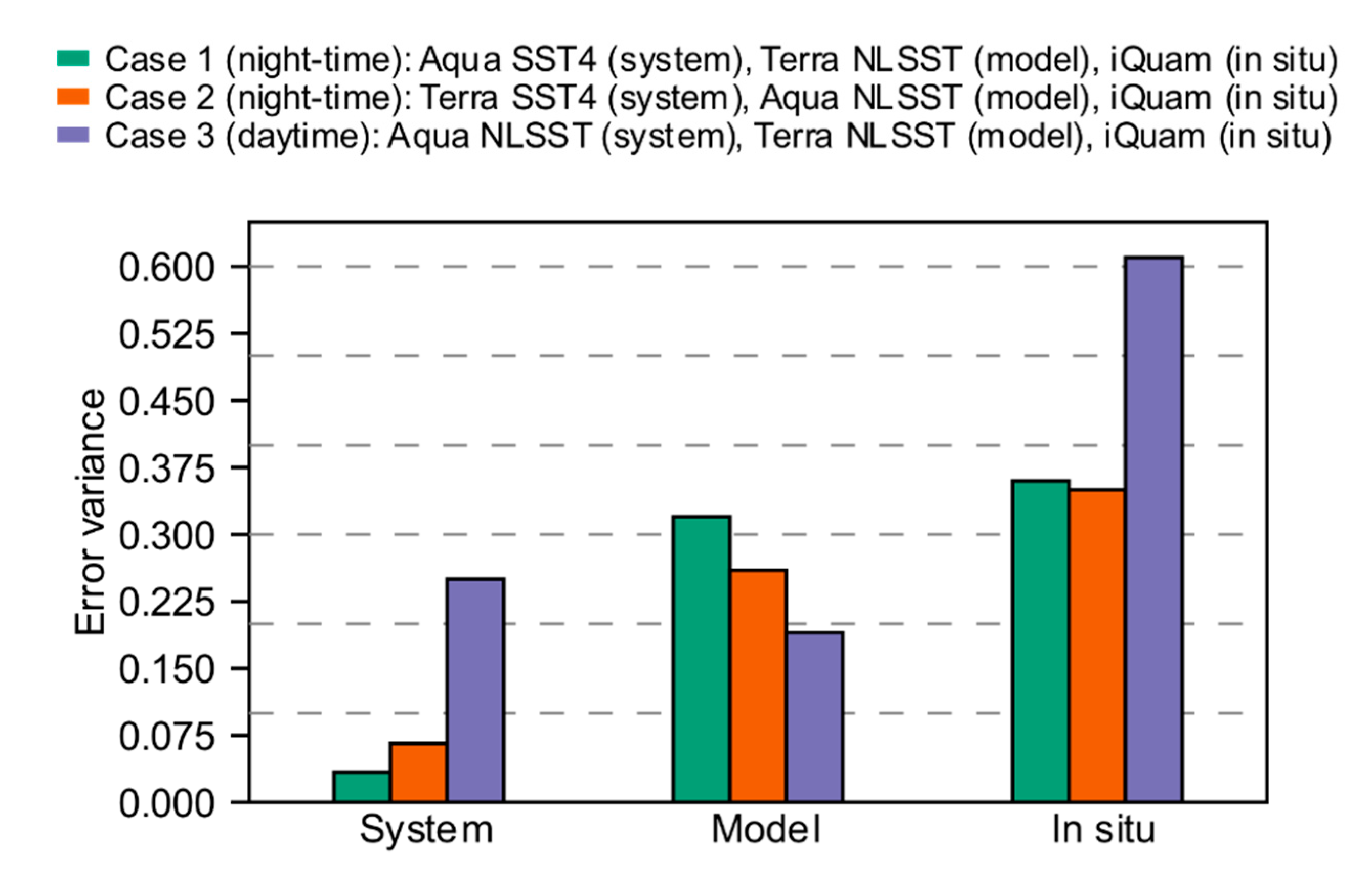
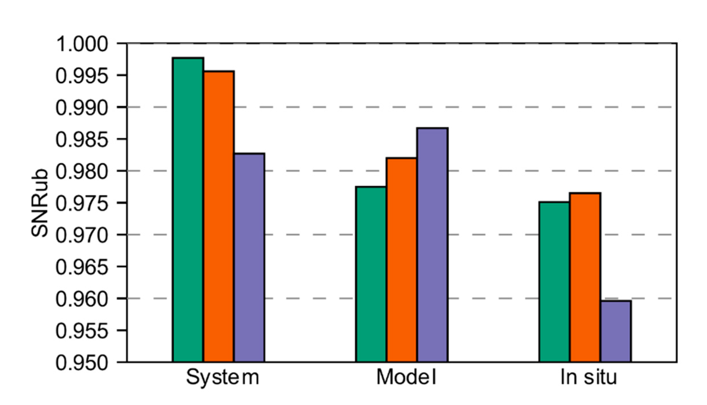
| 1 | Night-time (N = 3382) | Aqua | SST4 | 0.034 (0.18) | 0.9977 | 0.69 | 0.63 | 0.9728 |
| Terra | NLSST | 0.32 (0.57) | 0.9775 | 0.85 | 0.83 | 0.9532 | ||
| iQuam | — | 0.36 (0.60) | 0.9751 | — | — | — | ||
| 2 | Night-time (N = 3659) | Aqua | NLSST | 0.26 (0.51) | 0.9820 | 0.85 | 0.78 | 0.9590 |
| Terra | SST4 | 0.066 (0.26) | 0.9956 | 0.69 | 0.64 | 0.9721 | ||
| iQuam | — | 0.35 (0.59) | 0.9765 | — | — | — | ||
| 3 | Daytime (N = 5186) | Aqua | NLSST | 0.25 (0.50) | 0.9827 | 0.93 | 0.93 | 0.9430 |
| Terra | NLSST | 0.19 (0.44) | 0.9867 | 0.93 | 0.90 | 0.9469 | ||
| iQuam | — | 0.61 (0.78) | 0.9596 | — | — | — | ||
Publisher’s Note: MDPI stays neutral with regard to jurisdictional claims in published maps and institutional affiliations. |
© 2021 by the authors. Licensee MDPI, Basel, Switzerland. This article is an open access article distributed under the terms and conditions of the Creative Commons Attribution (CC BY) license (https://creativecommons.org/licenses/by/4.0/).
Share and Cite
Saleh, A.K.; Al-Anzi, B.S. Statistical Validation of MODIS-Based Sea Surface Temperature in Shallow Semi-Enclosed Marginal Sea: A Comparison between Direct Matchup and Triple Collocation. Water 2021, 13, 1078. https://doi.org/10.3390/w13081078
Saleh AK, Al-Anzi BS. Statistical Validation of MODIS-Based Sea Surface Temperature in Shallow Semi-Enclosed Marginal Sea: A Comparison between Direct Matchup and Triple Collocation. Water. 2021; 13(8):1078. https://doi.org/10.3390/w13081078
Chicago/Turabian StyleSaleh, Ali K., and Bader S. Al-Anzi. 2021. "Statistical Validation of MODIS-Based Sea Surface Temperature in Shallow Semi-Enclosed Marginal Sea: A Comparison between Direct Matchup and Triple Collocation" Water 13, no. 8: 1078. https://doi.org/10.3390/w13081078