
Smoothed Particle Hydrodynamics Simulations of Water Flow in a 90° Pipe Bend
by
 , , and
Leonardo Di G. Sigalotti
1,*,† ,
,
Carlos E. Alvarado-Rodríguez
2,3,† ,
,
Jaime Klapp
4 and
José M. Cela
5,† 1
Departamento de Ciencias Básicas, Universidad Autónoma Metropolitana-Azcapotzalco (UAM-A), Av. San Pablo 180, Ciudad de México 02200, Mexico
2
Dirección de Cátedras CONACYT, Av. Insurgentes Sur 1582, Crédito Constructor, Benito Juárez, Ciudad de México 03940, Mexico
3
Departamento de Ingeniería Química, DCNyE, Universidad de Guanajuato, Noria Alta S/N, Guanajuato 36000, Mexico
4
Instituto Nacional de Investigaciones Nucleares (ININ), Carretera México-Toluca km 36.5, La Marquesa, Ocoyoacac 52750, Mexico
5
Barcelona Supercomputing Center BSC-CNS, Campus Nord UPC, 08034 Barcelona, Spain
*
Author to whom correspondence should be addressed.
†
These authors contributed equally to this work.
Water 2021, 13(8), 1081; https://doi.org/10.3390/w13081081
Submission received: 21 March 2021
/
Revised: 3 April 2021
/
Accepted: 7 April 2021
/
Published: 14 April 2021
(This article belongs to the Section Hydraulics and Hydrodynamics)
Abstract
:The flow through pipe bends and elbows occurs in a wide range of applications. While many experimental data are available for such flows in the literature, their numerical simulation is less abundant. Here, we present highly-resolved simulations of laminar and turbulent water flow in a pipe bend using Smoothed Particle Hydrodynamics (SPH) methods coupled to a Large-Eddy Simulation (LES) model for turbulence. Direct comparison with available experimental data is provided in terms of streamwise velocity profiles, turbulence intensity profiles and cross-sectional velocity maps at different stations upstream, inside and downstream of the pipe bend. The numerical results are in good agreement with the experimental data. In particular, maximum root-mean-square deviations from the experimental velocity profiles are always less than ∼1.4%. Convergence to the experimental measurements of the turbulent fluctuations is achieved by quadrupling the resolution necessary to guarantee convergence of the velocity profiles. At such resolution, the deviations from the experimental data are ∼0.8%. In addition, the cross-sectional velocity maps inside and downstream of the bend shows that the experimentally observed details of the secondary flow are also very well predicted by the numerical simulations.
1. Introduction
Pipe bends and elbows are frequently used to fit pipeline systems. They are important in many engineering applications such as the transportation of oil and gas in pipelines as well as other fluids, including hot water and steam for shorter distances, water for drinking or irrigation over long distances and hydrogen from the point of delivery to the point of demand, just to mention a few applications. The flow in bends is complex and inherently unsteady due to the generation of secondary flows in the form of vortices as a result of centrifugal forces produced by the bend curvature [1,2,3]. This secondary flow can produce strong vibrations and mechanical fatigue of the pipe system. The strength of the secondary flow will depend on the radius of curvature of the pipe bend, , and the Reynolds number, Re , where is the bulk velocity, D is the pipe diameter and is the kinematic viscosity. Understanding its characteristics is important to determine the pressure losses and the heat/mass transfer in such bends, which are of considerable engineering importance. For example, visualization of turbulent motion in pipe flow has determined that flow separation occurs behind the bend inlet when , giving rise to increased pressure losses, while for a pair of counter-rotating vortices forms within the bend that force the cross-sectional contours of the streamwise flow velocity to become C-shaped and its profiles to substantially distort from parabolic flow as they are shifted away from the center of curvature of the bend [4].
Experimental investigations of laminar and turbulent flow in pipe bends of circular and square section have been reported by a number of authors in the last four decades [1,2,3,5,6,7,8,9,10]. An extensive review on theoretical, experimental and numerical work on flow in curved pipes spanning from 1839 to 2016 was reported by Kalpakli Vester et al. [11]. Some of these studies include numerical simulations of the experiments using commercial fluid flow softwares such as ANSYS Fluent and OpenFOAM. A numerical assessment of the characteristics of laminar flow in a elbow was undertaken by van de Vosse et al. [12] by adopting finite element methods and, more recently, by Pantokratoras [13] using ANSYS Fluent, who found that the velocity profiles at the bend inlet are shifted towards the inner pipe wall when the bend curvature is high, while they remain almost symmetric at low curvature. In addition, at high curvature and Reynolds numbers, the velocity profiles are shifted towards the outer pipe wall at the bend outlet and towards the inner wall at low Reynolds numbers, while when the curvature is low the velocity profiles are shifted towards the outer wall at the bend exit independently of the Reynolds number. Numerical simulations of turbulent flow in bends aimed at comparing the Large-Eddy Simulation (LES) approach with various Reynolds-averaged Navier–Stokes (RANS) turbulence models were reported by Röhrig et al. [14], while flow separation in such bends was numerically studied by Dutta et al. [15] using the RANS approach coupled to a model. In terms of the mean velocity profiles and turbulence intensities downstream of the bend outlet, the former authors found that LES provided much better agreement with the experimental data than the RANS approaches. Direct numerical simulations of turbulent flow in a pipe bend at Re were performed by Wang et al. [16] to investigate flow oscillation frequencies downstream of the bend and by Hufganel et al. [17] for flow at Re = 11,700 to study the nature of the three-dimensional wave-like structure that is responsible for the low-frequency switching affecting the Dean vortices downstream of the pipe bend and causing the fatigue of the pipe system. More recently, Du et al. [18] employed a LES turbulence model together with the proper orthogonal decomposition method to investigate the effects of varying the bend angle on pressure drop and mean flow characteristics in a small-diameter corrugated pipe. They found that increasing the bend angle from to produces stronger Dean vortices and increased pressure drops downstream of the pipe bend.
Flow simulations in curved pipes using Smoothed Particle Hydrodynamics (SPH) methods are much less abundant. The few examples found in the literature include the two-dimensional simulations by Hou et al. [19], who studied flow separation in right-angled bends for different turning angles; the three-dimensional SPH simulations by Alvarado-Rodríguez et al. [20], where the numerical results were compared with Sudo et al.’s [2] experimental measurements for turbulent flow in a square-sectioned pipe bend and Rup et al.’s [6] Fluent-based simulations of Sudo et al.’s experiment; and the calculations by Rosić et al. [21] aimed at testing the SPH capability to model supercritical flow across pipe bends. SPH is a fully Lagrangian, particle-based method that has become very popular in the last thirty years because of its many applications and ease of implementation [22,23,24]. In SPH, the state of the fluid is represented by a finite set of particles, where the physical properties carried by each particle are obtained from its close neighbors by means of an interpolation function, called the smoothing kernel. This way particles are allowed to interact with each other within the compact spherical support of the smoothing kernel. The resulting collective motion of the SPH particles mimics the flow of a fluid and so it can be modeled using the classical equations of hydrodynamics.
In this paper, we present the results of highly resolved SPH simulations of laser-Doppler velocimetry measurements of laminar and developing turbulent water flow in a pipe elbow reported by Enayet et al. [1]. These experiments were carried out for laminar flow at Re and 1093 and for turbulent flow at a maximum obtainable Re of 43,000. The SPH calculations were performed using a weakly compressible (WCSPH) scheme [25] coupled to a Large-Eddy Simulation (LES) model for turbulence and non-reflecting outflow boundary conditions at the pipe outlet [20]. The numerical results are compared with the experimental data for both types of flow in terms of mean velocity profiles upstream of the bend inlet, cross-sectional mean velocity maps at different angles within the bend and downstream of the bend exit and turbulence intensity profiles upstream of the bend for Re = 43,000. At spatial resolutions higher than that for which convergence to the experimental velocity profiles is guaranteed, the results reproduce Enayet et al.’s [1] measurements with root-mean-square deviations %. In particular, the wall static pressure variation within the bend and the turbulence intensity profiles upstream of the bend inlet for Re = 43,000 are remarkably well reproduced by the SPH simulations when the resolution needed to guarantee convergence of the velocity profiles to the experimental data is quadrupled.
In what follows, the governing equations and a brief outline of the numerical framework are given in Section 2, while Section 3 describes the pipe flow model. Section 4 presents the numerical results by providing direct comparison with Enayet et al.’s [1] experiments and Section 5 summarizes the relevant conclusions.
2. Governing Equations and Numerical Framework
2.1. Exact Equations
Under prescribed inlet, outlet and solid wall boundary conditions, the differential equations describing the flow in a bent pipe are given by the Navier–Stokes equations
where is the fluid density, is the flow velocity vector, p is the pressure, m s is the kinematic viscosity of water at 20 C and is the gravitational acceleration. To complete the governing equations, the Murnaghan–Tait equation of state is employed where the pressure and density are related according to
where for water, , kg m is the water density at 20 C and is a numerical sound speed taken to be at least 10 times higher than the maximum flow velocity in order to ensure weak compressibility and fluctuations of the density field [25]. This enforces the incompressibility condition because the effects of any compression induced by such density fluctuations will be purely acoustic and superimposed to the main flow with almost no interaction.
2.2. LES Filtering
In the LES approach, the flow velocity must be separated into its mean component (or resolved scale) velocity, namely , and its fluctuating component (or sub-particle scale) velocity, , such that . The mean velocity is obtained by means of the density-weighted Favre-filtering
where T is a sufficiently large time interval and is the Reynolds-averaged density. After application of the Favre filtering, Equations (1) and (2) become
Here, is the sub-particle stress tensor defined by
where is the Favre-filtered strain rate tensor given by
, , with , is the Smagorinsky eddy viscosity, is the local strain rate, is the Kronecker delta and is a measure of the finite particle size. For practical purposes, is set equal to the local particle smoothing length h. A form of that improves the stress–strain relationship is given by , where is dynamically determined as a function of the smallest resolved scales [26]. The choice of the LES model is based on the results of the comparative assessment performed by Röhrig et al. [14] between the LES and various RANS models for turbulent flow in a pipe elbow. In particular, they found that LES reproduced the experimental velocity profiles and the turbulent intensities in the streamwise direction much better than the RANS schemes. On the other hand, it is well known that, for flow problems where experimental data are not available, LES is in general employed to generate reference data for the calibration and validation of turbulence closures.
2.3. The SPH Method
The Favre-filtered Equations (5) and (6) are solved using a variant of the DualSPHysics code [27]. Equation (5) is solved for the density fluctuations using the SPH representation
where is the particle-scale density, is the kernel function, is the smoothing length of particle a, is the mass of neighboring particle b and the summation is taken over all neighbors of particle a within the compact support of the kernel, i.e., for . The subscript a in the nabla operator means that the derivatives of the kernel function must be taken with respect to the coordinates of particle a. The tilde operator over the ensemble average velocity vector and the bar operator over the mean density have been dropped for simplicity. In SPH form, the momentum Equation (6) is given by
where the symmetric form suggested by Colagrossi and Landrini [28] is employed for the pressure gradient term and those used by Lo and Shao [29] are adopted for the laminar viscous term and the sub-particle stresses. In particular, the form of the pressure gradient with a positive sign is chosen on the basis that it is variationally consistent with the use of Equation (9) for the density [30]. Here, and . To prevent the growth of numerical errors due to anisotropies in the spatial distribution of particles, they are moved along the pipe section using the equation [31]
where , is the maximum estimated fluid velocity, M is the total mass of fluid within the pipe and is given by
where the summations in Equations (11) and (12) are taken over all fluid particles in the computational domain.
2.4. Boundary Conditions
The fluid flow in a truncated pipe requires the treatment of boundary conditions at the pipe inlet, the pipe outlet and the solid wall. No-slip boundary conditions () are implemented at the solid wall using the method of dynamic boundary particles proposed by Crespo et al. [34,35]. In this work, a layer of particles defines the pipe wall and two layers of ghost particles are placed outside the computational domain around the pipe wall. These outer boundary particles are treated as normal fluid particles. Although they are updated using Equation (10), they are forced to remain stationary and preserve their initial positions. The density of the wall and outer boundary particles is determined by the density of all neighboring fluid particles lying within their support domains. To avoid particle penetration across the pipe wall, the wall particles will exert artificial repulsive forces to nearby fluid particles, which are derived from the source of the momentum Equation (10).
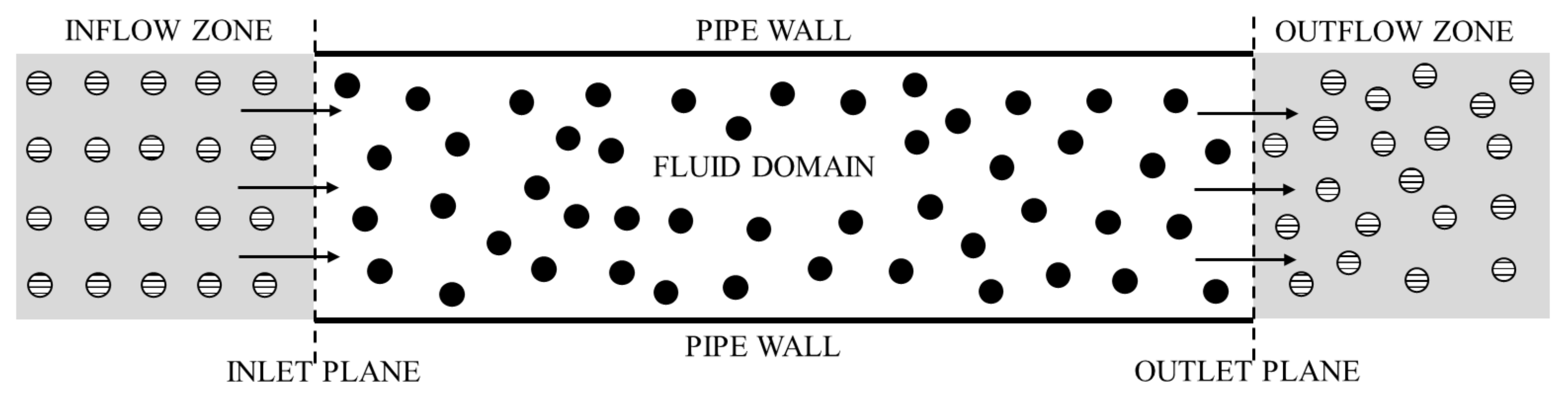
The pipe inlet and outlet are treated as open boundary conditions. Proper inlet boundary conditions are implemented by placing an inflow zone in front of the entrance plane, as shown in Figure 1. The inflow zone is filled with five columns of regularly distributed particles and has a length equal to , where is the initial fluid particle separation in the flow direction. Inflow particles are then allowed to flow in as needed with a prescribed density and velocity. This way boundary information propagates into the flow domain since fluid particles close to the inlet plane will use information from neighboring inflow particles lying within their support domains. The outlet boundary is treated using non-reflecting outflow boundary conditions [20]. This method requires defining an outflow zone in front of the outlet plane of the same length as the inflow zone (see Figure 1). Fluid particles entering the outflow zone are moved by solving the outgoing wave equation
where . In this equation, the assumption is made that the streamwise flow is in the x-direction. Since the inflow rate may differ from the outflow rate, the number of particles entering and leaving the fluid domain may not be the same. Therefore, particles leaving the outflow zone are stored in a reservoir buffer zone with a zero velocity. This way, when an inflow particle crosses the inlet plane and enters the fluid domain, a particle is removed from the buffer and placed into the inflow zone. At the beginning of a simulation, the reservoir buffer is not necessarily empty but must contain an arbitrary number of stationary particles as needed.
A numerically stable SPH representation of Equation (14) is given by
where the subscript o is employed to denote outflow particles, , , and . The numerical stability of Equation (15) can be improved if the streamwise velocity of outflowing particles, , is smoothed according to the summation
which is equivalent to averaging the convective velocity close to the outlet plane. Since for outflow particles nearby the outlet plane the summations in Equations (15) and (16) will include both types of particles (i.e., fluid and outflow particles) the information carried by fluid particles crossing the outlet plane is propagated outwards so that feedback noise from the outlet boundary is greatly reduced. As a final remark, the position of outflow particles is determined by solving the equation
which must be integrated using the same loop as the inner fluid particles.
2.5. Time Marching Scheme
The temporal integration of Equations (9)–(11) is performed using a second-order Verlet scheme, which is implemented according to the following difference formulae
where . To improve the numerical coupling among Equations (9)–(11) during the evolution, the above scheme is replaced every 40 timesteps by the alternative differences
To ensure numerical stability, the time step is constrained by the following criteria
where the maximum and minima are taken over all particles in the system, is the sound speed for particle a given by
and
is the magnitude of the fluid acceleration obtained by direct evaluation of the source terms in Equation (10).
3. Pipe Bend Model Description
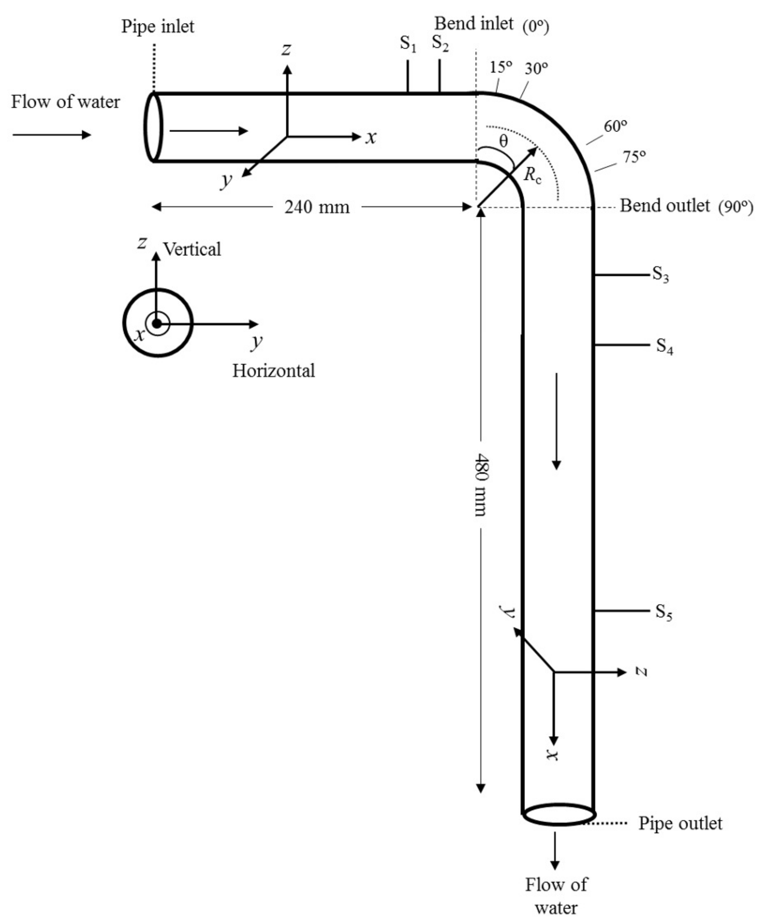
The flow configuration investigated here corresponds to the experimental test bend analyzed by Enayet et al. [1]. This represents a pipe of diameter mm, which is turned around an angle of with a radius of curvature mm, as depicted in Figure 2. Consistent entrance and exit flow is established by attaching the bend to linear piping. Straight pipes of length mm and mm are attached to the bend upstream of its inlet plane and downstream of its outlet plane, respectively. The numerical simulations were aimed at reproducing the laser-Doppler data acquired by Enayet et al. [1]. To do so, the simulations were carried out for three different sets of inlet conditions, corresponding to flat inlet streamwise velocities: (a) mm s (Re ); (b) mm s (Re ); and (c) m s (Re = 43,000). For these models, the mass flow rate is calculated according to
and the bulk velocity is given by
To enforce direct comparison with the experimental data, flow measurements are made at the pipe stations and upstream of the bend inlet, corresponding to distances from the pipe inlet of 192 and 212.16 mm, respectively, at angles , , and inside the bend, and at stations , and downstream of the bend outlet, corresponding to distances of 432, 384 and 192 mm from the pipe exit, respectively.
Important quantities that must be compared with the experimental data for Re = 43,000 are the turbulence intensity and the pressure coefficient given by
where is the wall static pressure measured in station . In particular, we are interested in the turbulence intensity in the streamwise direction. In turbulent flow, the streamwise velocity can be separated into its mean value, , and its fluctuating part, , such that , where is calculated as a mean over time, i.e.,
Here, T is a sufficiently long time interval which can be set equal to the time required to achieve a stationary flow. From knowledge of , the turbulent fluctuation in the streamwise direction follows as
The turbulence intensity is defined as the root-mean-square (rms) of the square of the fluctuating velocity, namely
so that
which gives the turbulence intensity in the streamwise direction.
Validation and Particle Independence Test
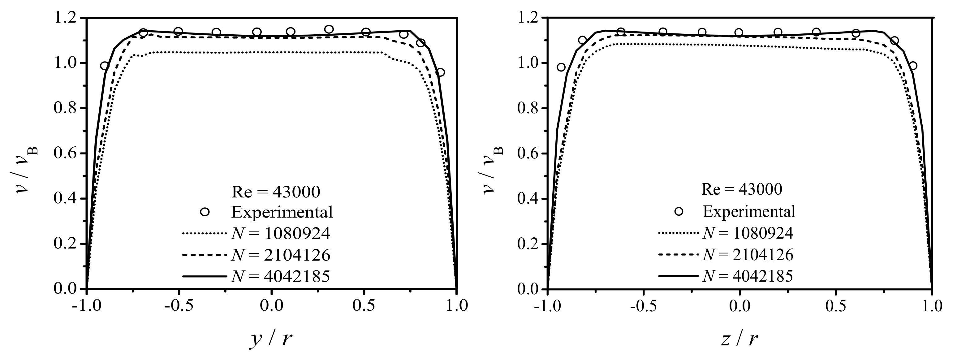
For validation purposes, the same geometrical configuration of Figure 2 was adopted in preliminary simulations, which were optimized via a convergence study by increasing the number of SPH fluid particles. Figure 3 shows the results of the convergence study for varying spatial resolution from 1,080,924 to 4,042,185 particles, where the streamwise velocity profiles in the horizontal (y) and vertical (z) planes normalized to are compared with Enayet et al.’s [1] experimental measurements at pipe station for Re = 43,000. Asymptotic convergence to the experimental data is observed for 4,042,185 particles. At this resolution, the root-mean-square (RMSE) deviations between the numerical results and the experimental data are ≈1.3% for the horizontal profile and ≈1.4% for the vertical profile.
4. Results
The validation test was performed to assess convergence to the experimental streamwise velocity profiles at pipe station upstream of the bend for Re = 43,000. Further comparison of the numerical results with Enayet et al.’s [1] measurements at different angles within the bend and stations downstream of the bend outlet was performed by further increasing the spatial resolution to 8,064,442 and 16,056,513 particles. In particular, Enayet et al.’s experimental measurements were considered to be accurate enough to provide a useful benchmark test for checking the numerical accuracy of any flow prediction method.
4.1. Laminar Flow
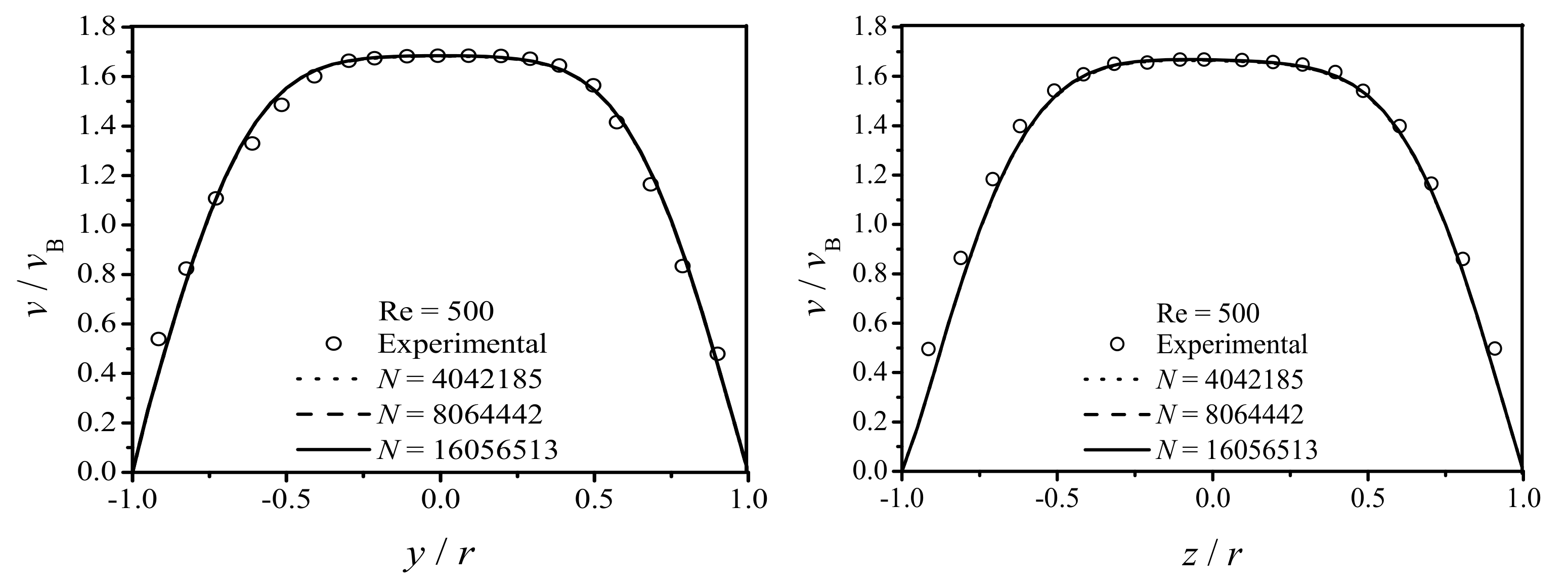
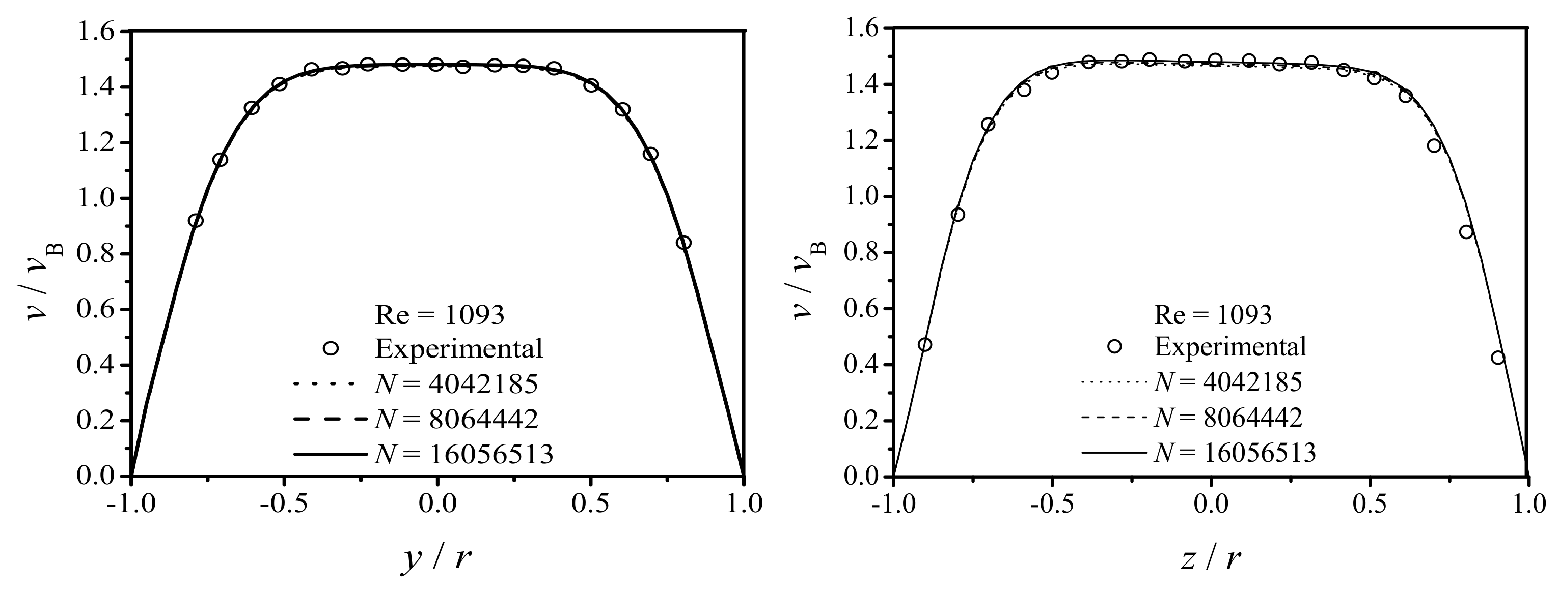
For laminar flow at Re, Figure 4 shows the horizontal (left) and vertical (right) streamwise velocity profiles as compared with the experimental measurements at upstream of the bend inlet. The same plots for Re are displayed in Figure 5. The profiles for 4,042,185, 8,064,442 and 16,056,513 particles closely overlap each other and match the experimental data with RMSE deviations ≲0.8%. When the Reynolds number is doubled from 500 to 1093, the thickness of the inlet boundary layer decreases from ≈0.26D to ≈0.23D, resulting in a larger central region (potential core) of uniform velocity. These features are also in very good agreement with the experimental observations.
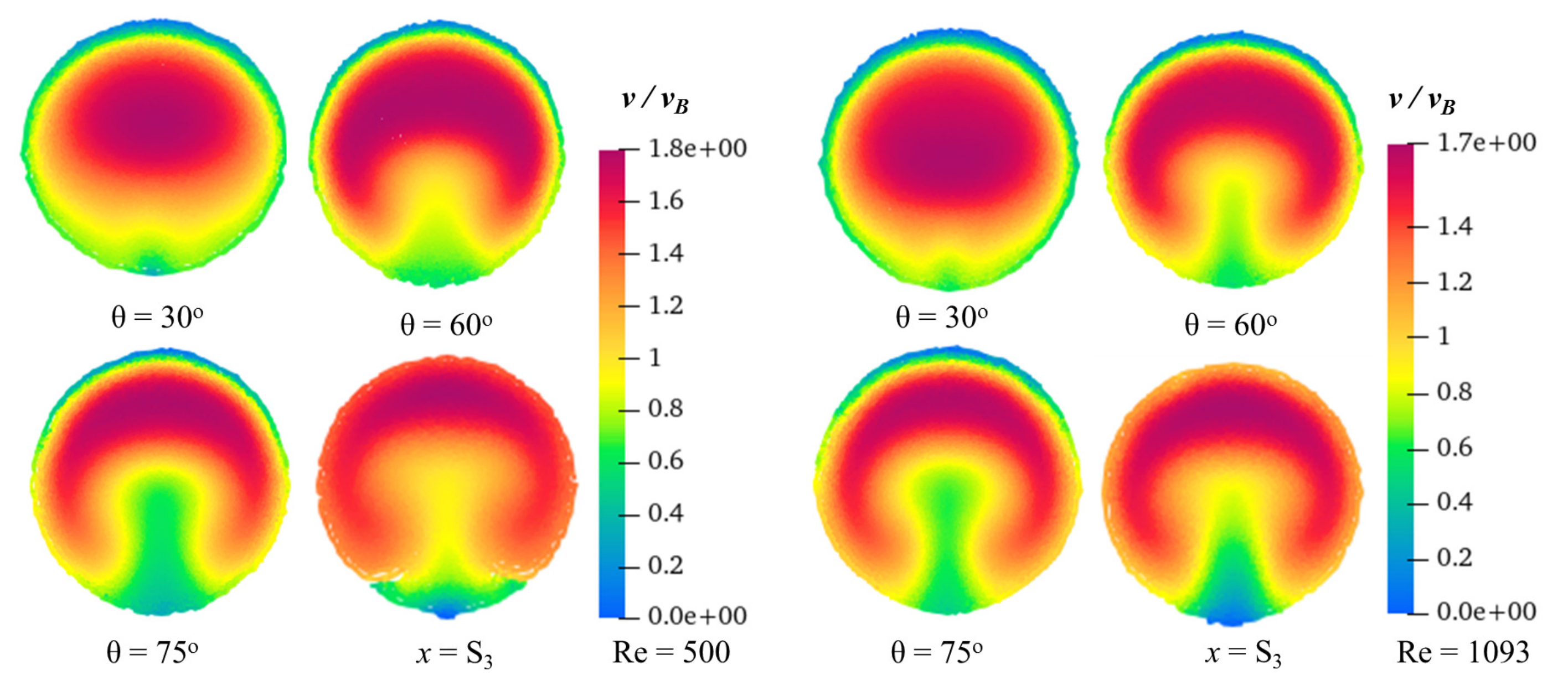
Figure 6 shows maps of the streamwise velocity for Re (left) and 1093 (right) in three cross-stream planes at , and in the bend and at downstream of the bend outlet for the 16,056,513 run. Almost indistinguishable plots to Figure 6 were also obtained for 8,064,442 particles. The velocity maps reproduce the shape of Enayet et al.’s [1] experimental contours at the same stations and the values of associated with the colors in the maps fit very well their contour level numbers (see their Figure 4 and Figure 6). As a result of doubling the Reynolds number, the transverse pressure gradient within the bend increases and, as a consequence, the secondary flow becomes more intense. In both cases, the secondary flow develops gradually and displaces the core region of maximum velocity to the outer arc of the bend. At the plane, a thickening of the shear layer towards the inner arc of the bend is already visible. This effect is greater for Re than for Re . When the flow crosses the plane, the secondary flow is almost fully developed in both cases, leading to a C-shaped distortion of the core and a displacement of the peak velocity from the plane of symmetry. Owing to the increased centrifugal forces and transverse pressure gradients, the secondary flow is stronger for the Re case. At , the flow distortion is such that the region of maximum velocity takes a horseshoe shape, which is more clearly defined for Re than for Re because of the more intense swirling secondary flow in the former case. At the exit of the bend, the secondary motion persists and does not show a significant decay at station downstream of the bend outlet, as shown in Figure 6.
4.2. Turbulent Flow
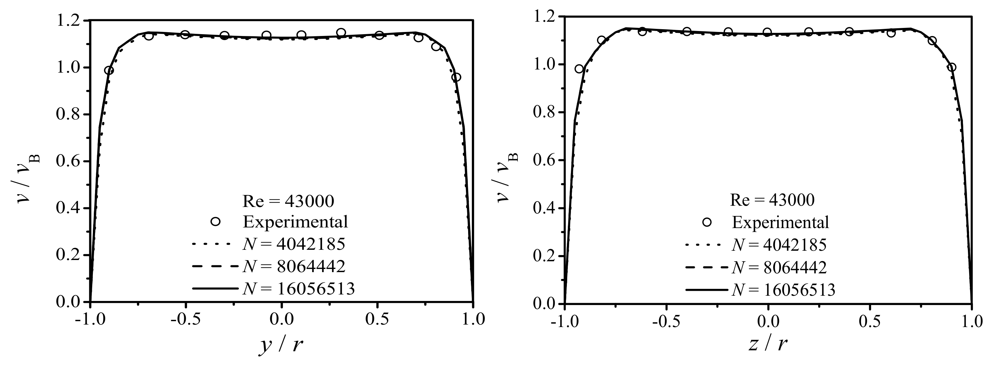
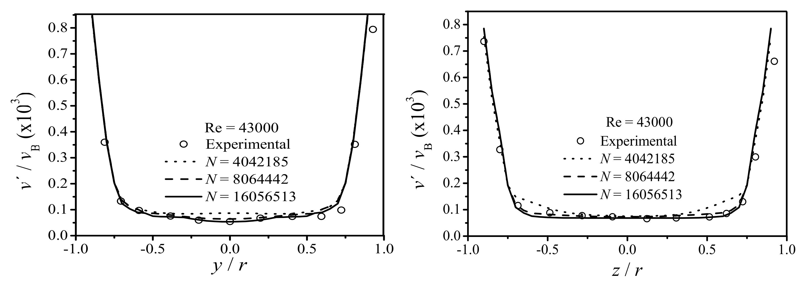
At Re = 43,000, the inlet boundary layers are turbulent. Figure 7 displays the horizontal (left) and vertical (right) streamwise velocity profiles for 4,042,185, 8,064,442 and 16,056,513 particles as compared to the experimental measurements (empty circles) at upstream of the bend inlet. As in Figure 4 and Figure 5 for the laminar flows, at these high resolutions, the profiles closely overlap each other, meaning that the simulations are well inside the convergence region. It is evident from the results in Figure 7 that, when passing from Re to Re = 43,000, the inlet boundary layers become much thinner. The simulations predict a thickness of ≈0.09D, which is in good agreement with the experimental observations for the same turbulent flow. As a consequence of the slimming of the inlet boundary layers, the region of maximum (uniform) velocity at the center of the pipe section becomes much larger, extending over most of the pipe diameter. The RMSE deviation of the numerical profiles from the experimental data is always less than about 0.7%. The horizontal and vertical profiles of the streamwise velocity rms fluctuations (turbulence intensity) are displayed in Figure 8. While asymptotic convergence for the streamwise velocity profiles in both the laminar and turbulent approach flows 0.58 pipe diameters upstream of the bend inlet is always achieved with 4,042,185 particles, Figure 8 shows that the same level of convergence for the rms fluctuations needs to quadruple the number of particles. This clearly means that the turbulent fluctuations are by far more sensitive to resolution than the streamwise flow. The turbulence intensity is minimum in the potential core region and increases in the inlet boundary layers where the flow is turbulent. The numerical simulations match the experimental data for the turbulence intensity with RMSE deviations which are always ≲0.8% when 16,056,513.
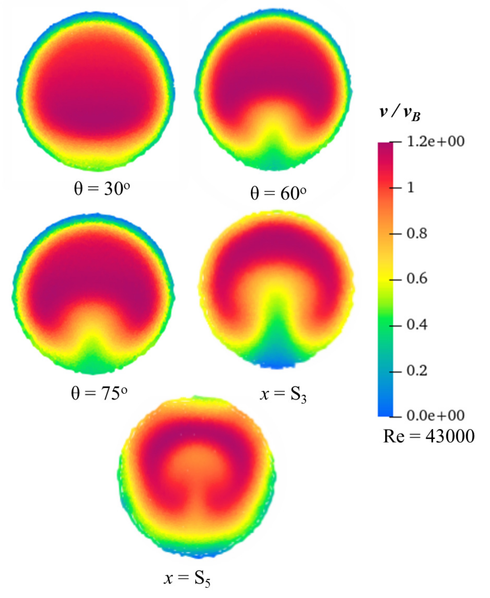
Cross-sectional maps of the streamwise velocity are shown in Figure 9 for , and in the bend and in planes and downstream of the bend outlet. By the cross-sectional plane, the region of maximum velocity (potential core) was displaced towards the inside of the bend as a result of the adjustment of the flow to the cross-stream pressure gradient imposed by the bend curvature. This feature is in perfect agreement with the experimental contours of Enayet et al. (their Figure 9). At and , the potential core looks highly distorted due to the presence of a strong swirling secondary flow, which is largely confined near the inner wall of the pipe where the velocity gradients are steeper and grows with distance through the bend. Close to the bend exit, the secondary flow extends over the entire cross-sectional area. However, downstream of the bend outlet, the transverse pressure gradients disappear, causing the velocity peak to move towards the outer wall as shown at pipe station . In contrast to laminar flow, where a C-shaped core forms within the bend, in turbulent flow, the core becomes C-shaped at the exit of the pipe bend. The secondary flow persists down the straight pipe section and at station the potential core embraces most of the pipe circular cross-section and deforms into a well-pronounced horseshoe shape.
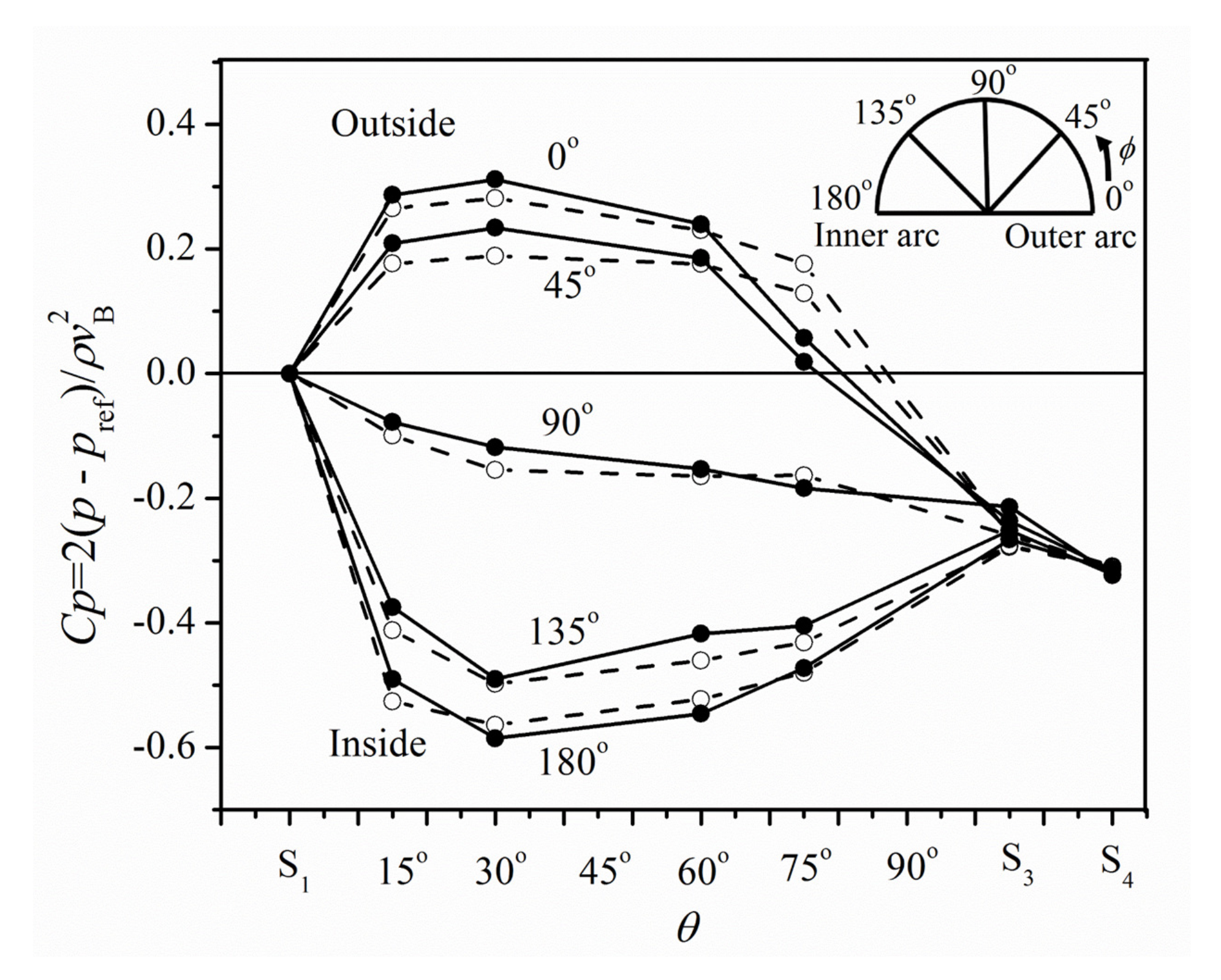
The static pressure at the pipe wall can be calculated using Equation (26) as a function of position along the pipe and azimuthal angle on the circular pipe wall. At Re = 43,000, the variation of the pressure coefficient is sufficiently large to allow for accurate experimental measurements of the wall static pressure. To provide a comparison with the experimentally obtained results of Enayet et al. (their Figure 7), we calculate the pressure coefficient at azimuthal angles , ,, and on the circular wall, as shown by the inset of Figure 10, at stations upstream of the bend inlet, at cross-sections , , and in the bend and at stations and in the straight pipe section downstream of the bend outlet.
It is clear from the results in Figure 10 that the variation of the static wall pressure declines rapidly at about one diameter from the bend exit. The numerical results (filled circles) match fairly well the experimental data (open circles) with RMSE deviations between ∼1.8 () and ∼0.8% (). An interesting experimental observation which is reproduced by the numerical simulations is that the negative pressure variation (at on the inner arc of the bend) is approximately twice the positive pressure gradient on the opposite side, i.e., at on the outer arc of the bend. The form of the pressure coefficient across the bend reveals the sequences of favorable to adverse pressure gradient along the inner and outer arcs of the bend. A comparison of both sequences shows that the pressure variation is stronger along the inner arc, which is a common feature for this type of flow.
5. Conclusions
The laminar and turbulent flows of water through a pipe bend were simulated numerically using Smoothed Particle Hydrodynamics (SPH) techniques coupled to a large-eddy simulation (LES) approach and non-reflective outflow boundary conditions at the pipe exit. The simulations were addressed to embody a comparative assessment of how well the proposed SPH method can predict the laser-Doppler measurements of water flow in a pipe elbow reported by Enayet et al. [1].
For laminar flow at Re and 1093, the SPH simulations were able to reproduce the experimental streamwise velocity profiles upstream of the bend inlet with sufficiently good accuracy. For a total number of particles ≥4,042,185, the numerically obtained profiles were seen to deviate from the experimental data with root-mean-square errors (RMSE) that were always less than 1%. Similar accurate results were also obtained for the velocity profiles upstream of the bend inlet at Re = 43,000. At this Re-value, the simulations predict that the inlet boundary layer is turbulent and much thinner (≈0.09D, where D is the pipe diameter) than that for the laminar case at Re (≈0.23D), which in both cases matched the experimentally measured values. Although asymptotic convergence to the experimental streamwise velocity profiles was already achieved for 4,042,185 particles for both laminar and turbulent flows, it was necessary to increase the resolution to 16,056,513 particles to observe the same level of convergence for the turbulence intensity profiles in the streamwise direction close to the bend inlet. At such high resolution, the numerically obtained profiles were seen to deviate from the experimental data with RMSE errors of ∼0.8%. Moreover, the details of the flow structure through the bend, concerning the strength of the swirling secondary flow and the deformation of the potential core, were also very well predicted by the present SPH simulations. Intensity velocity maps at different cross-sectional planes within the bend were seen to accurately match the experimentally obtained contour levels, showing that the occurring secondary flow can be precisely captured by the SPH simulations. Another important quantity characterizing the flow in curved pipes is the variation of the wall static pressure along the inner and outer arc of the bend. This provides information about the pressure gradients at different stations on the bend wall. The numerical simulations predicted the experimentally measured wall static pressures with RMSE deviations between ∼0.8 and ∼1.8% and reproduced very well the dependence of the pressure coefficient with position across the bend. The numerical solutions indicate that global convergence to the results of the experimental test bend analyzed by Enayet et al. [1] with the present SPH scheme requires working with a minimum of 16 million particles to correctly reproduce the behavior of resolution-sensitive quantities, such as the turbulence intensity and the variation of the wall static pressure, when coupling the scheme to a LES model. The good agreement demonstrated between the numerical solution and the experimental data for varying Re shows that the present SPH scheme can handle turbulent flows with pronounced streamline curvatures and potential separation regions with an acceptably good degree of prediction.
Author Contributions
Conceptualization, L.D.G.S. and J.K.; methodology, L.D.G.S. and C.E.A.-R.; software, C.E.A.-R.; validation, L.D.G.S., C.E.A.-R. and J.K.; formal analysis, L.D.G.S.; resources, J.K. and J.M.C.; data curation, C.E.A.-R.; writing—original draft preparation, L.D.G.S.; writing—review and editing, L.D.G.S. and J.K.; visualization, C.E.A.-R.; supervision, J.K.; project administration, J.M.C., J.K. and L.D.G.S.; and funding acquisition, J.K. and J.M.C. All authors have read and agreed to the published version of the manuscript.
Funding
This research was funded by the European Union’s Horizon 2020 Programme under the ENERXICO Project grant number 828947 and under the Mexican CONACYT-SENER-Hidrocarburos grant number B-S-69926 and by CONACYT under project number 368’.
Acknowledgments
The calculations of this study were performed using computational facilities at the Barcelona Supercomputer Center (BSC) and ABACUS-Laboratorio de Matemática Aplicada y Cómputo de Alto Rendimiento of Cinvestav.
Conflicts of Interest
The authors declare no conflict of interest. The funders had no role in the design of the study; in the collection, analyses, or interpretation of data; in the writing of the manuscript, or in the decision to publish the results.
References
- Enayet, M.M.; Gibson, M.M.; Taylor, A.M.K.P.; Yianneskis, M. Laser-Doppler measurements of laminar and turbulent flow in a pipe bend. Int. J. Heat Fluid Flow 1982, 3, 213–219. [Google Scholar] [CrossRef] [Green Version]
- Sudo, K.; Sumida, M.; Hibara, H. Experimental investigation on turbulent flow in a circular-sectioned 90-degree bend. Exp. Fluids 1998, 25, 42–49. [Google Scholar] [CrossRef]
- Sudo, K.; Sumida, M.; Hibara, H. Experimental investigation on turbulent flow in a square-sectioned 90-degree bend. Exp. Fluids 2001, 30, 246–252. [Google Scholar] [CrossRef]
- Hellström, L.H.O.; Sinha, A.; Smits, A.J. Visualizing the very-large-scale motion in turbulent pipe flow. Phys. Fluids 2011, 23, 011703. [Google Scholar] [CrossRef] [Green Version]
- Verma, A.K.; Singh, S.N.; Seshadri, V. Pressure drop for the flow of high concentration solid-liquid mixture across 90° horizontal coventional circular pipe bend. Indian J. Eng. Mat. Sci. 2006, 13, 477–483. [Google Scholar]
- Rup, K.; Malinowski, L.; Sarna, P. Measurements of flow rate in square-sectioned duct bend. J. Theoret. Appl. Mech. 2011, 49, 301–311. [Google Scholar]
- Kalpakli, A.; Örlü, R. Turbulent pipe flow downstream a 90° pipe bend with and without superimposed swirl. Int. J. Heat Fluid Flow 2013, 41, 103–111. [Google Scholar] [CrossRef]
- Kim, J.; Yadav, M.; Kim, S. Characteristics of secondary flow induced by 90-degree elbow in turbulent pipe flow. Eng. Appl. Comput. Fluid Mech. 2014, 8, 229–239. [Google Scholar] [CrossRef]
- Wang, S.; Ren, C.; Sun, Y.; Yang, X.; Tu, J. A study on the instantaneous turbulent flow field in a 90-degree elbow pipe with circular section. Sci. Tech. Nucl. Inst. 2016, 2016, 5265748. [Google Scholar] [CrossRef]
- Kalpakli Vester, A.; Sattarzadeh, S.S.; Örlü, R. Combined hot-wire and PIV measurements of a swirling turbulent flow at the exit of a 90° pipe bend. J. Vis. 2016, 19, 261–273. [Google Scholar] [CrossRef]
- Kalpakli Vester, A.; Örlü, R.; Alfredsson, P.H. Turbulent flows in curved pipes: Recent advances in experiments and simulations. Appl. Mech. Rev. 2016, 68, 050802. [Google Scholar] [CrossRef]
- Van de Vosse, F.N.; van Steenhoven, A.A.; Segal, A.; Janssen, J.D. A finite element analysis of the steady laminar entrance flow in a 90° curved tube. Int. J. Numer. Meth. Fluids 1989, 9, 275–287. [Google Scholar] [CrossRef]
- Pantokratoras, A. Steady laminar flow in a 90° bend. Adv. Mech. Eng. 2016, 8, 1–9. [Google Scholar] [CrossRef]
- Röhrig, R.; Jakirlić, S.; Tropea, C. Comparative computational study of turbulent flow in a 90° pipe elbow. Int. J. Heat Fluid Flow 2015, 55, 120–131. [Google Scholar] [CrossRef]
- Dutta, P.; Saha, S.K.; Nandi, N.; Pal, N. Numerical study on flow separation in 90° pipe bend under high Reynolds number by k-ϵ modelling. Eng. Sci. Technol. Int. J. 2016, 19, 904–910. [Google Scholar]
- Wang, Z.; Orlü, R.; Schlatter, P.; Chung, Y.M. Direct numerical simulation of a turbulent 90° bend pipe flow. Int. J. Heat Fluid Flow 2018, 73, 199–208. [Google Scholar] [CrossRef] [Green Version]
- Hufganel, L.; Canton, J.; "Orlü, R.; Marin, O.; Merzari, E.; Schlatter, P. The three-dimensional structure of swirl-switching in bent pipe flow. J. Fluid Mech. 2018, 835, 86–101. [Google Scholar]
- Du, X.; Wei, A.; Fang, Y.; Yang, Z.; Wei, D.; Lin, C.-H.; Jin, Z. The effect of bend angle on pressure drop and flow behavior in a corrugated duct. Acta Mech. 2020, 231, 3755–3777. [Google Scholar] [CrossRef]
- Hou, Q.; Kruisbrink, A.C.H.; Pearce, F.R.; Tijsseling, A.S.; Yue, T. Smoothed particle hydrodynamics simulations of flow separation at bends. Comput. Fluids 2014, 90, 138–146. [Google Scholar] [CrossRef] [Green Version]
- Alvarado-Rodríguez, C.E.; Klapp, J.; Sigalotti, L.D.G.; Domínguez, J.M.; de la Cruz Sánchez, E. Nonreflecting outlet boundary conditions for incompressible flows using SPH. Comput. Fluids 2017, 159, 177–188. [Google Scholar] [CrossRef] [Green Version]
- Rosić, N.M.; Kolarević, M.B.; Savić, L.M.; Dordević, D.M.; Kapor, R.S. Numerical modelling of supercritical flow in circular conduit bends using SPH method. J. Hydrodyn. 2017, 29, 344–352. [Google Scholar] [CrossRef]
- Monaghan, J.J. Smoothed particle hydrodynamics. Annu. Rev. Astron. Astrophys. 1992, 30, 543–574. [Google Scholar] [CrossRef]
- Liu, M.B.; Liu, G.R. Smoothed particle hydrodynamics (SPH): An overview and recent developments. Arch. Comput. Meth. Eng. 2010, 17, 25–76. [Google Scholar] [CrossRef] [Green Version]
- Monaghan, J.J. Smoothed particle hydrodynamics and its diverse applications. Annu. Rev. Fluid Mech. 2012, 44, 323–346. [Google Scholar] [CrossRef]
- Becker, M.; Teschner, M. Weakly compressible SPH for free surface flows. In Proceedings of the 2007 ACM SIGGRAPH/Europhysics Symposium on Computer Animation, San Diego, CA, USA, 2–4 August 2007; ACM Press: San Diego, CA, USA, 2007; pp. 32–58. [Google Scholar]
- Germano, M.; Piomelli, U.; Moin, P.; Cabot, W.H. A dynamic subgrid scale eddy viscosity model. Phys. Fluids 1991, 3, 1760–1765. [Google Scholar] [CrossRef] [Green Version]
- Gómez-Gesteira, M.; Rogers, B.D.; Crespo, A.J.C.; Dalrymple, R.A.; Narayanaswamy, M.; Domínguez, J.M. Sphysics—Development of a free-surface fluid solver—Part 1: Theory and formulations. Comput. Geosci. 2012, 48, 289–299. [Google Scholar] [CrossRef]
- Colagrossi, A.; Landrini, M. Numerical simulation of interfacial flows by smoothed particle hydrodynamics. J. Comput. Phys. 2003, 191, 448–475. [Google Scholar] [CrossRef]
- Lo, E.Y.M.; Shao, S. Simulation of near-shore solitary wave mechanics by an incompressible SPH method. Appl. Ocean Res. 2002, 24, 275–286. [Google Scholar]
- Bonet, J.; Lok, T.-S.L. Variational and momentum preservation aspects of smooth particle hydrodynamic formulations. Comput. Meth. Appl. Mech. Eng. 1999, 180, 97–115. [Google Scholar] [CrossRef]
- Vacondio, R.; Rogers, B.D.; Stansby, P.K.; Mignosa, P.; Feldman, J. Variable resolution for SPH: A dynamic particle coalescing and splitting scheme. Comput. Meth. Appl. Mech. Eng. 2013, 256, 132–148. [Google Scholar] [CrossRef]
- Wendland, H. Piecewise polynomial, positive definite and compactly supported radial functions of minimal degree. Adv. Comput. Math. 1995, 4, 389–396. [Google Scholar] [CrossRef]
- Dehnen, W.; Aly, H. Improving convergence in smoothed particle hydrodynamics simulations without pairing instability. Mon. Not. R. Astron. Soc. 2012, 425, 1068–1082. [Google Scholar] [CrossRef] [Green Version]
- Crespo, A.J.C.; Gómez-Gesteira, M.; Dalrymple, R.A. Boundary conditions generated by dynamic particles in SPH methods. Comput. Mat. Cont. 2007, 5, 173–184. [Google Scholar]
- Crespo, A.J.C.; Domínguez, J.M.; Rogers, B.D.; Gómez-Gesteira, M.; Longshaw, S.; Canelas, R.; Vacondio, R.; Barreiro, A.; García-Feal, O. DualSPHysics: Open-source parallel CFD solver based on smoothed particle hydrodynamics (SPH). Comput. Phys. Commun. 2015, 187, 204–216. [Google Scholar] [CrossRef]
Figure 1.
Illustration of the inlet and outlet boundary treatment.

Figure 2.
Schematic diagram of the bend geometry and dimensions. The vertical lines on the outer arc of the pipe mark the stations where the numerical results are compared with the experimental data.
Figure 2.
Schematic diagram of the bend geometry and dimensions. The vertical lines on the outer arc of the pipe mark the stations where the numerical results are compared with the experimental data.

Figure 3.
Numerical horizontal (left) and vertical (right) streamwise velocity profiles for 1,080,924, 2,104,126 and 4,042,185 particles as compared with the experimental data at upstream of the bend inlet for Re = 43,000. Asymptotic convergence of the numerical solution to the experimental measurements is obtained for 4,042,185 SPH particles.

Figure 4.
Comparison of the numerical normalized horizontal (left) and vertical (right) streamwise velocity profiles with the experimental measurements at upstream of the bend inlet for Re and 4,042,185, 8,064,442 and 16,056,513 particles.
Figure 4.
Comparison of the numerical normalized horizontal (left) and vertical (right) streamwise velocity profiles with the experimental measurements at upstream of the bend inlet for Re and 4,042,185, 8,064,442 and 16,056,513 particles.

Figure 5.
Comparison of the numerical normalized horizontal (left) and vertical (right) streamwise velocity profiles with the experimental measurements at upstream of the bend inlet for Re and 4,042,185, 8,064,442 and 16,056,513 particles.
Figure 5.
Comparison of the numerical normalized horizontal (left) and vertical (right) streamwise velocity profiles with the experimental measurements at upstream of the bend inlet for Re and 4,042,185, 8,064,442 and 16,056,513 particles.

Figure 6.
Cross-sectional streamwise velocity maps at planes , and through the bend and downstream of the bend outlet for Re (left) and Re (right). The numbers on the color bars indicate the values of the streamwise velocity normalized to .
Figure 6.
Cross-sectional streamwise velocity maps at planes , and through the bend and downstream of the bend outlet for Re (left) and Re (right). The numbers on the color bars indicate the values of the streamwise velocity normalized to .

Figure 7.
Comparison of the numerical normalized horizontal (left) and vertical (right) streamwise velocity profiles with the experimental measurements at upstream of the bend inlet for Re = 43,000 and 4,042,185, 8,064,442 and 16,056,513 particles.
Figure 7.
Comparison of the numerical normalized horizontal (left) and vertical (right) streamwise velocity profiles with the experimental measurements at upstream of the bend inlet for Re = 43,000 and 4,042,185, 8,064,442 and 16,056,513 particles.

Figure 8.
Comparison of the numerical normalized horizontal (left) and vertical (right) turbulence intensity profiles with the experimental measurements at upstream of the bend inlet for Re = 43,000 and 4,042,185, 8,064,442 and 16,056,513 particles.
Figure 8.
Comparison of the numerical normalized horizontal (left) and vertical (right) turbulence intensity profiles with the experimental measurements at upstream of the bend inlet for Re = 43,000 and 4,042,185, 8,064,442 and 16,056,513 particles.

Figure 9.
Cross-sectional streamwise velocity maps at planes , and in the bend and at stations and downstream of the bend outlet for Re = 43,000. The numbers on the color bars indicate the values of the streamwise velocity normalized to .
Figure 9.
Cross-sectional streamwise velocity maps at planes , and in the bend and at stations and downstream of the bend outlet for Re = 43,000. The numbers on the color bars indicate the values of the streamwise velocity normalized to .

Figure 10.
Variation of the wall static pressure along the inner and outer arc of the bend at Re = 43,000. The numerically calculated values (filled dots) are compared with Enayet et al.’s [1] experimental measurements (open circles). The data are taken at station upstream of the bend inlet, at angles , , and in the bend and at stations and downstream of the bend outlet for azimuthal angles , , , and on the circular wall of the pipe.

Publisher’s Note: MDPI stays neutral with regard to jurisdictional claims in published maps and institutional affiliations. |
© 2021 by the authors. Licensee MDPI, Basel, Switzerland. This article is an open access article distributed under the terms and conditions of the Creative Commons Attribution (CC BY) license (https://creativecommons.org/licenses/by/4.0/).
Share and Cite
MDPI and ACS Style
Sigalotti, L.D.G.; Alvarado-Rodríguez, C.E.; Klapp, J.; Cela, J.M. Smoothed Particle Hydrodynamics Simulations of Water Flow in a 90° Pipe Bend. Water 2021, 13, 1081. https://doi.org/10.3390/w13081081
AMA Style
Sigalotti LDG, Alvarado-Rodríguez CE, Klapp J, Cela JM. Smoothed Particle Hydrodynamics Simulations of Water Flow in a 90° Pipe Bend. Water. 2021; 13(8):1081. https://doi.org/10.3390/w13081081
Chicago/Turabian StyleSigalotti, Leonardo Di G., Carlos E. Alvarado-Rodríguez, Jaime Klapp, and José M. Cela. 2021. "Smoothed Particle Hydrodynamics Simulations of Water Flow in a 90° Pipe Bend" Water 13, no. 8: 1081. https://doi.org/10.3390/w13081081
Note that from the first issue of 2016, this journal uses article numbers instead of page numbers. See further details here.