
An Empirical Analysis of Sediment Export Dynamics from a Constructed Landform in the Wet Tropics


1
Centre for Water in the Minerals Industry, Sustainable Minerals Institute, The University of Queensland, Brisbane, QLD 4072, Australia
2
School of Civil Engineering, The University of Queensland, Brisbane, QLD 4072, Australia
3
Geotechnical and Hydrological Engineering Research Group, Federation University Churchill, Churchill, VIC 3841, Australia
*
Author to whom correspondence should be addressed.
Water 2021, 13(8), 1087; https://doi.org/10.3390/w13081087
Submission received: 9 March 2021
/
Revised: 1 April 2021
/
Accepted: 2 April 2021
/
Published: 15 April 2021
(This article belongs to the Section Water Erosion and Sediment Transport)
Abstract
:Although plot-scale erosion experiments are numerous, there are few studies on constructed landforms. This limits the understanding of their long-term stability, which is especially important for planning mined land rehabilitation. The objective of this study was to gain insight into the erosion processes in a 30 × 30 m trial plot on a mine waste rock dump in tropical northern Australia. The relationships between rainfall, runoff and suspended and bedload sediment export were assessed at annual, seasonal, inter-event and intra-event timescales. During a five-year study period, 231 rainfall–runoff–sediment export events were examined. The measured bedload and suspended sediments (mainly represented in nephelometric turbidity units (NTU)) showed the dominance of the wet season and heavy rainfall events. The bedload dominated the total mass, although the annual bedload diminished by approximately 75% over the five years, with greater flow energy required over time to mobilise the same bedload. The suspended load was more sustained, though it also exhibited an exhaustion process, with equal rainfall and runoff volumes and intensities, leading to lower NTU values over time. Intra-event NTU dynamics, including runoff-NTU time lags and hysteretic behaviours, were somewhat random from one event to the next, indicating the influence of the antecedent distribution of mobilisable sediments. The value of the results for supporting predictive modelling is discussed.
1. Introduction
Soil erosion can be exacerbated in newly constructed landforms with negative consequences on-site and downstream. Constructing new landforms is inherent to mining projects; hence, the management of erosion is a continual challenge for the mining industry. Even after mining activities have stopped, erosion continues in the associated constructed landforms, including waste rock dumps and tailings storage facilities. Riley [1] reported the unmanaged surface of a waste rock dump to be 10 to 100 times more erodible than neighbouring natural hillslopes and [2] described a mosaic of landforms due to the erosion of abandoned tailing deposits. Other examples are provided by [3,4]. The global erosivity analysis of [5] shows that landforms in tropical climates may be especially susceptible.
Soil erosion processes, including particle separation, transfer and sedimentation, have been well studied, e.g., [6,7]. The dominant drivers of these processes are rainfall and runoff, with factors including rainfall and runoff intensity, infiltration, soil properties and slope grade and length [8,9,10]. The kinetic energy and intensity of rainfall are dominant controlling characteristics. While many studies on this subject have been conducted using a constant rainfall intensity [11], the importance of intensity variations, in particular peak intensity, has also been addressed [12,13,14,15,16]. Sediment loss from storms with constant intensity may be less than that from storms of varying intensity [17], and higher rainfall intensity close to the end of the storm may increase the amount of runoff and soil loss. Shen et al., Flanagan et al. and Tao et al. [13,18,19] investigated the effects of different rainfall pattern types (uniform, increasing, increasing–decreasing and decreasing) on sediment load generation using four plots with 15° slopes and rainfall intensities of 100, 130 and 160 mm/h. The results showed that the rainfall intensity had a significant effect on the runoff generation process, the erosion process and the total amount of sediment. Early high rainfall intensity was shown to be a likely cause of the most severe erosion. Other experimental studies have shown that the amount of sediment erosion may increase linearly with the surface slope, and hence, the runoff energy, as well as with the rainfall energy [20,21]. Interactions between the runoff and sediments and surface roughness can also be important via its effects on the runoff energy; furthermore, ripping of the land surface can alter runoff pathways, velocities and the spatial distribution of particle sizes [22,23,24].
Soil erosion studies have covered various scales from experimental plots to large catchments [25,26,27,28,29,30,31]. Plot scale experiments help to examine, under controlled and relatively well-measured conditions, the variables (rainfall–runoff, erosivity, soil erodibility, slope length, etc.) affecting erosion rates [32]. Besides rainfall and runoff intensity effects, insights into various other effects, including rilling, rainfall and vegetation cover, have been offered [33,34,35,36,37], while observed changes in the runoff–sediment relationship has provided insight into their interaction mechanisms [38]. Experimental plots can have limitations in exploring larger-scale processes, such as gully formation [39,40]; nevertheless, they can be considered an essential part of observing the underlying processes and erosion rates, as well as how they respond to land management options.
A good understanding of landform erosion processes is essential for successful mine rehabilitation design [41]. Erosion rates from recently constructed mined landforms are likely to be higher because of the absence of established vegetation, the landscaped surface and modified soil properties, which are often defined by the available crushed waste rock and include large amounts of coarse stones [42]. These mine wastes generally have poor water storage capacity, low organic matter content, low nutrient content and low microbial activity, and may have high levels of heavy metals [42,43]. Saynor and Erskine [44] showed an exponential decline in the bedload in the early years following landform construction. In a temperate continental monsoon environment, [45] investigated the dynamic processes of soil erosion by simulating runoff on engineered landforms, concluding that stream power was the main driver of erosion, while different hydrodynamic parameters show varying degrees of effectiveness when describing soil detachment processes. Their reliance on simulations highlights the lack of appropriate observed data sets to test process hypotheses. Verbist et al. [46] used the observed bedload and suspended load to compare factors affecting soil loss at the plot and catchment scales, concluding that landslides, riverbank erosion and spatially concentrated erosion were the dominant processes. They showed that the relationship between the sediment yield and scale was nonlinear. Of these relevant plot-scale studies, the investigations by [43,47] are the only ones that used observed data from constructed landform plots. Despite the importance of a better understanding of constructed landform erosion processes, access to sites that would provide suitable experimental plots is rare [48].
The objective of this study was to build on the previous study of [43] to gain new insight into the variability and performance of plot-scale erosion of a constructed landform over multiple time scales (10-min to annual intervals). Specifically, the study primarily aimed to empirically quantify the relative importance of sediment exhaustion and rainfall and runoff event properties on both the suspended solid and bedload export rates. This study also explored the intra-event suspended sediment dynamics. The dominant processes that should be considered in erosion modelling and management of relevant landforms were inferred from the results.
2. Study Area
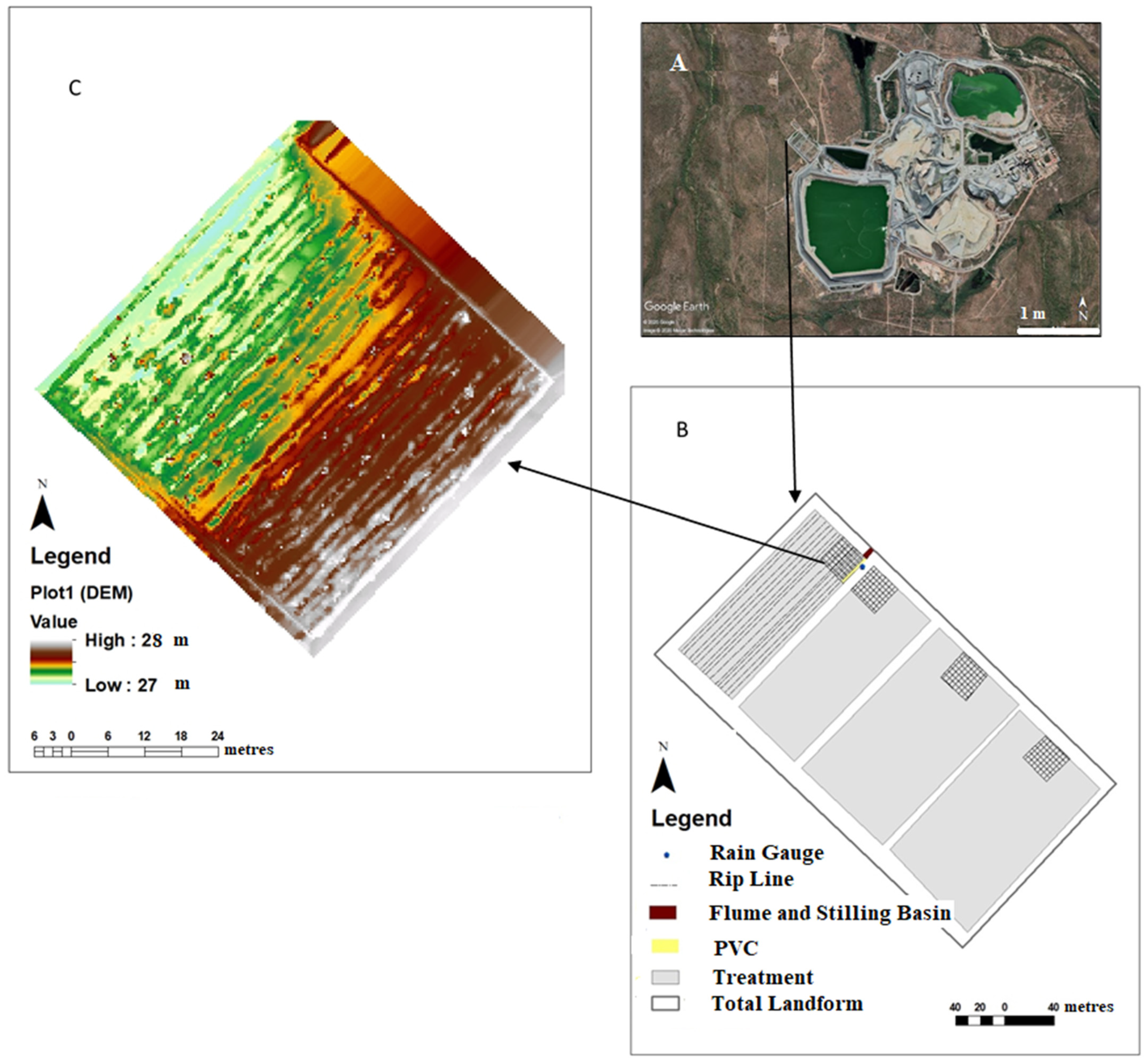
The studied mined landscape was at the Ranger Uranium Mine, which covers an area of approximately 6 km2 in Australia’s Northern Territory (Figure 1), located at 12°41′ S 132°55′ E. The mine is on Aboriginal land (Mirarr country) and is surrounded by the World-Heritage-listed Kakadu National Park. The long-term annual average rainfall is 1553 mm [49]. On average, 97% of the annual rainfall occurs during a distinct wet season from October to April. Short, high-intensity storms are common and, as a result, water erosion is the main erosion process [50].
Mining has ceased at the mine and it is in the decommissioning phase, which is planned to be completed by early 2026. Legislation requires that the Ranger Project area must be rehabilitated to establish an environment that is similar to the adjacent areas of the Kakadu National Park such that the rehabilitated area could be incorporated into the park. One of the main objectives of the environmental requirements for the closure of the mine is that the constructed landform should have “erosion characteristics which, as far as can reasonably be achieved, do not vary significantly from those of comparable landforms in surrounding undisturbed areas” [50].
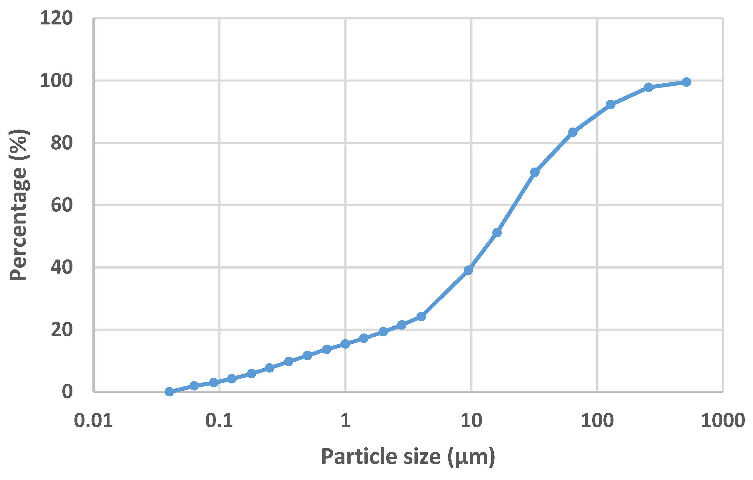
The Ranger trial landform was 8 hectares (200 × 400 m) and located to the north-west of the tailings storage facility. Four runoff plots, each approximately 30 × 30 m in size, were set up on the trial landform during the dry season of 2009 [43]. Plot 1 (Figure 1A) was the focus of this study as it had the most complete set of measured data. In plot 1, the landform was covered by waste rock, which was ripped along the contours to reduce runoff velocities. Figure 2 shows the particle size distribution for waste rock on the trial landform [51]. The average slope in the downslope direction (Figure 1) was approximately 2%. Tube stock planting was implemented in 2009 and significant growth was observed by 2016 [52].
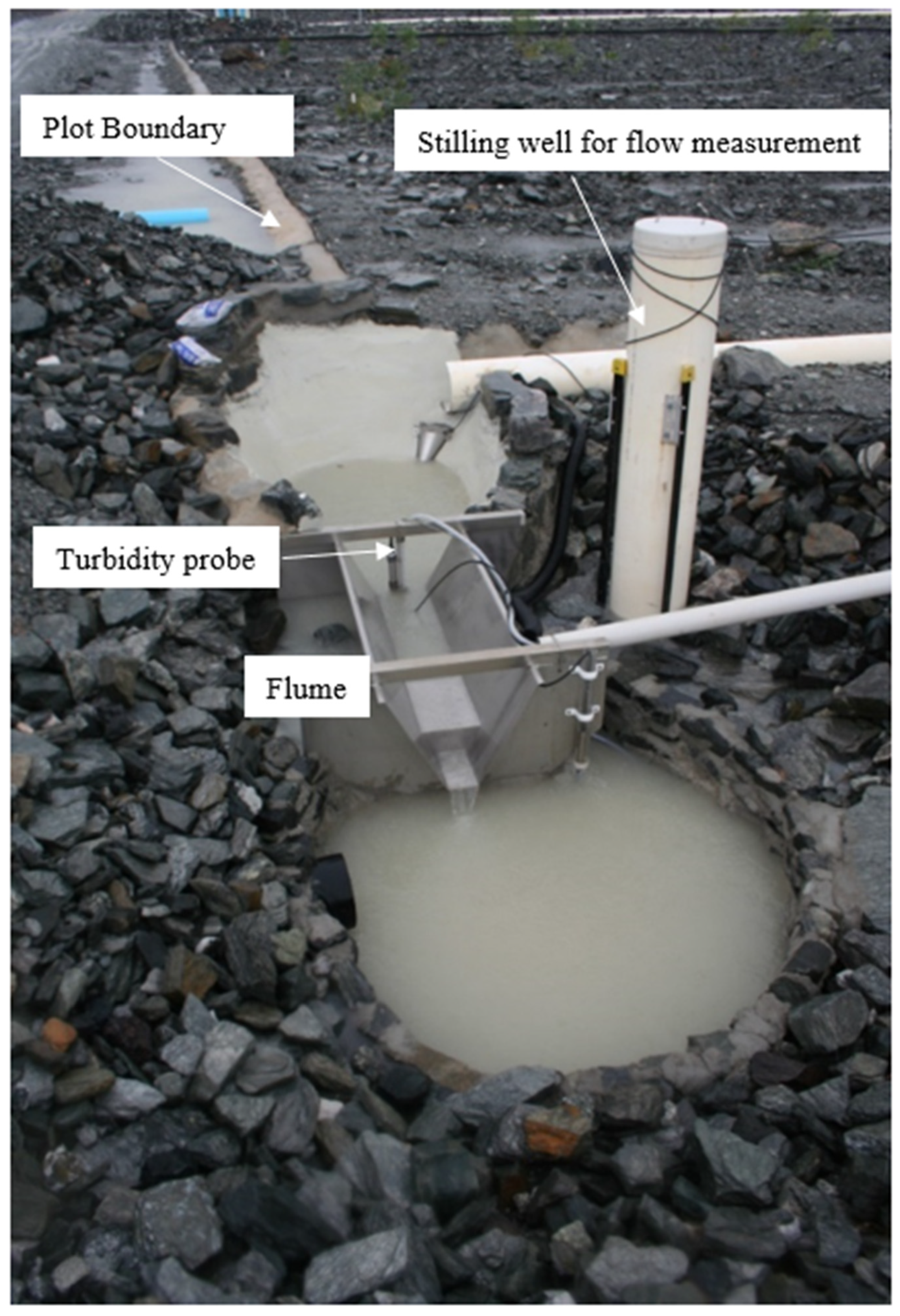
The plot was surrounded by concrete borders on three sides to isolate it from runoff from the upslope landform area. On the fourth (downslope) side, a polyvinyl chloride (PVC) half-tube was used to create a channel to capture the surface runoff. This drained to a runoff measurement flume. Both an optical shaft encoder (primary sensor) and pressure transducer (backup sensor) were used to measure the head upstream of the flume’s control section [43]. Rainfall was measured using a tipping bucket pluviometer adjacent to the plot. A turbidity probe (nephelometer) was positioned at the entry to the flume. The initial nephelometer, with a measurement range of 0 to 1000 NTU (nephelometric turbidity units), was replaced in February 2010 with a new probe with a range of 0 to 5000 NTU to also capture higher NTU values. Water samples during events were collected using an automatic sampler, which was triggered by electrical conductivity and turbidity. Selected samples were analysed for a range of parameters, including the total suspended sediment concentration [43]. Immediately upstream of the flume was a sediment trap (Figure 3). The bedload was deposited in both the half-pipe and the sediment trap. The bedload mass over the 5 years (2009–2014) was measured at weekly to monthly intervals, typically 3-week intervals. It was not measured after each runoff event due to resource constraints.
3. Methods of Data Analysis
Rainfall and runoff data (10-min totals), turbidity data (instantaneous values at 10-s intervals during runoff events), total suspended solids data (a total of 921 spot samples) and accumulated bedload masses (59 collection dates) were supplied by the ERISS (Environmental Research Institute of the Supervising Scientist) for the five hydrological years from September 2009 to August 2014 (the water year is defined as 1 September through to 31 August the following year).
The 1-min turbidity data (each an average of 10 readings) were filtered to remove any measurements up to February 2010 that were not considered reliable because they were above or near (within 100 NTU) the upper measurement limit (22 measurements removed). The remaining values were averaged over 10-min intervals that were synchronised with the rainfall–runoff total intervals. Gaps in the data meant that a total of 20% of the nonzero runoff period did not have corresponding turbidity data.
Suspended sediment concentrations (SSCs) were infilled using the SSC–runoff relationships (described in Appendix A) for the purpose of estimating the annual suspended sediment loads, while the untransformed 10-min NTU data were used for the analysis of the inter-event and intra-event suspended sediment dynamics. Annual suspended sediment loads were calculated as the 10-min runoff values multiplied by the corresponding infilled 10-min SSC values, summed over each of the five hydrological years and expressed in kilograms.
The data were primarily explored visually, with supporting regression analyses made wherever useful. First, the inter-annual and inter-seasonal variability and trends were plotted using the 10-min interval data. This was done to find evidence of sediment source exhaustion and the relative importance of the suspended sediment and the bedload. Second, the relationship between the measured bedload and runoff was plotted.
The rainfall–runoff events were then extracted. To delineate the continuous rainfall data into discrete events, the start of an event was the start of the rainfall that led to runoff, and the end of the event was when both the rainfall and runoff ceased and remained zero for the next 120 min, where 120 min was chosen to be short enough to limit the number and duration of multipeak events. A shorter delineation gap of 60 min was also analysed but did not significantly alter the results. Events with turbidity (NTU) data for less than 50% of the time steps were not considered. Events within which the turbidity data had a high (>50) or low (<2) coefficient of variance often contained a few unrealistically high values (either extreme step-ups and step-downs or a sequence of near-constant values that were inconsistent with the rainfall–runoff dynamics). All events in that coefficient of variance range were inspected visually and were disqualified if they were considered to be of suspicious quality. Nineteen events were excluded for this reason.
The remaining event data (turbidity (NTU), rainfall and runoff data) were analysed to understand the differences between events. The event-averaged (runoff-weighted) turbidity data were plotted against the runoff and rainfall event statistics: volume, average intensity, duration and maximum intensity. The aim was to indicate the relative importance of the runoff and rainfall energy controls on sediment detachment and transport, as previously investigated in the studies of [19,53].
The final stage of the analysis was the analysis of time lags between the peak turbidity and rainfall and the peak turbidity and runoff, along with plotting the rainfall time series, runoff and turbidity for selected events. This provided an exploration of whether event dynamics, including the presence and nature of hysteresis and the presence of early or late rainfall peaks, influenced the turbidity [54]. The 12 largest events in terms of peak rainfall intensity (all greater than 15 mm/10 min) with complete turbidity data were selected for plotting.
4. Results
4.1. Rainfall and Runoff Summary
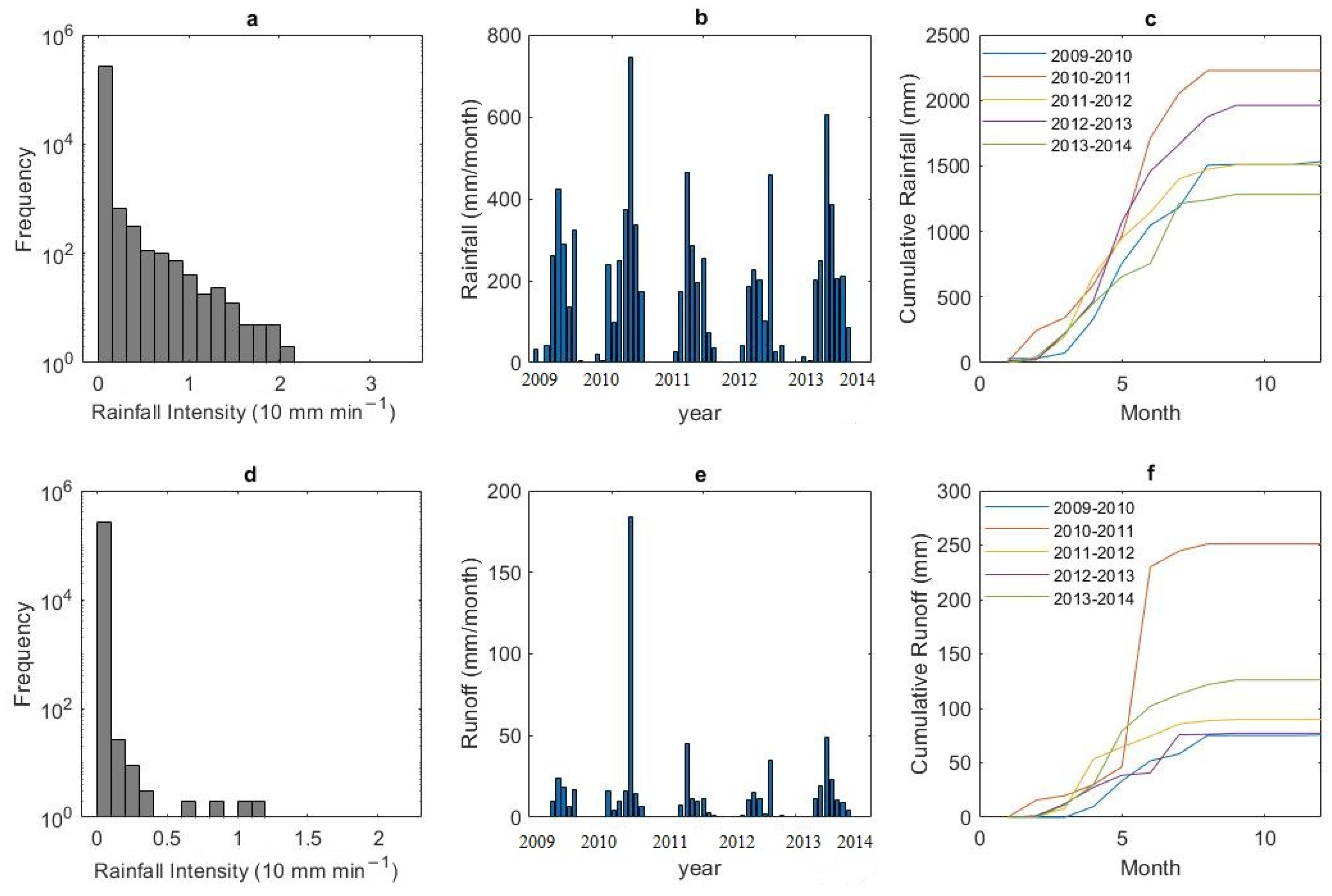
The frequency distribution of the rainfall, runoff and respective cumulative values during the experimental period are shown in Figure 4. Figure 4c shows that 2010–2011 (rainfall total of 2226 mm) was an above-average wet year relative to the average annual rainfall of 1553 mm and contained one month (February) with approximately 750 mm of rainfall compared to the long-term average for that month of 353 mm. The same month had the highest total runoff of 183 mm. The 10-min rainfall intensities shown are generally not exceptional compared to the long-term medians [50]; however, the 3-h event in February 2011 of 180 mm has annual return period that is greater than 100 years [22].
4.2. Annual and Seasonal Variability
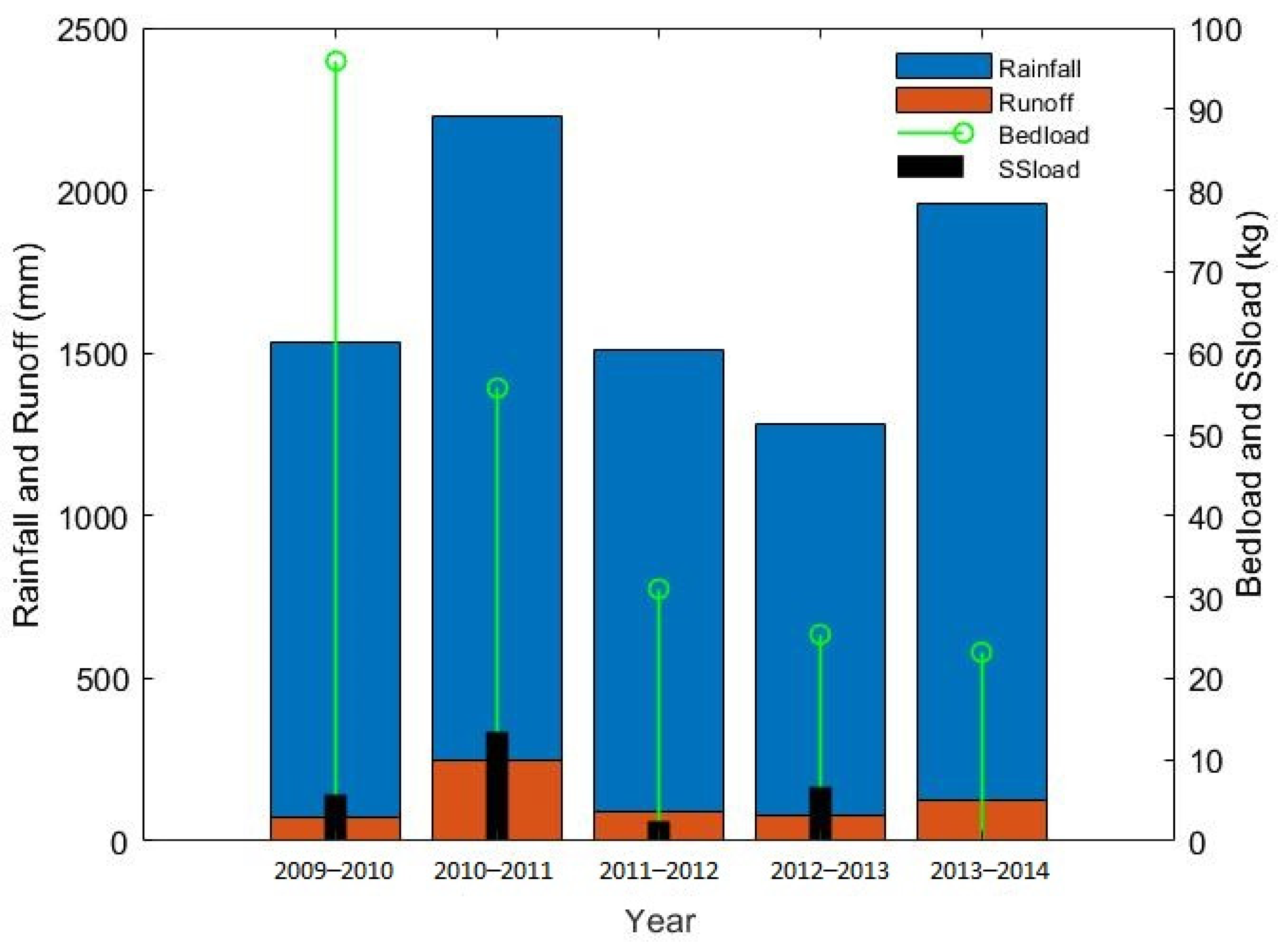
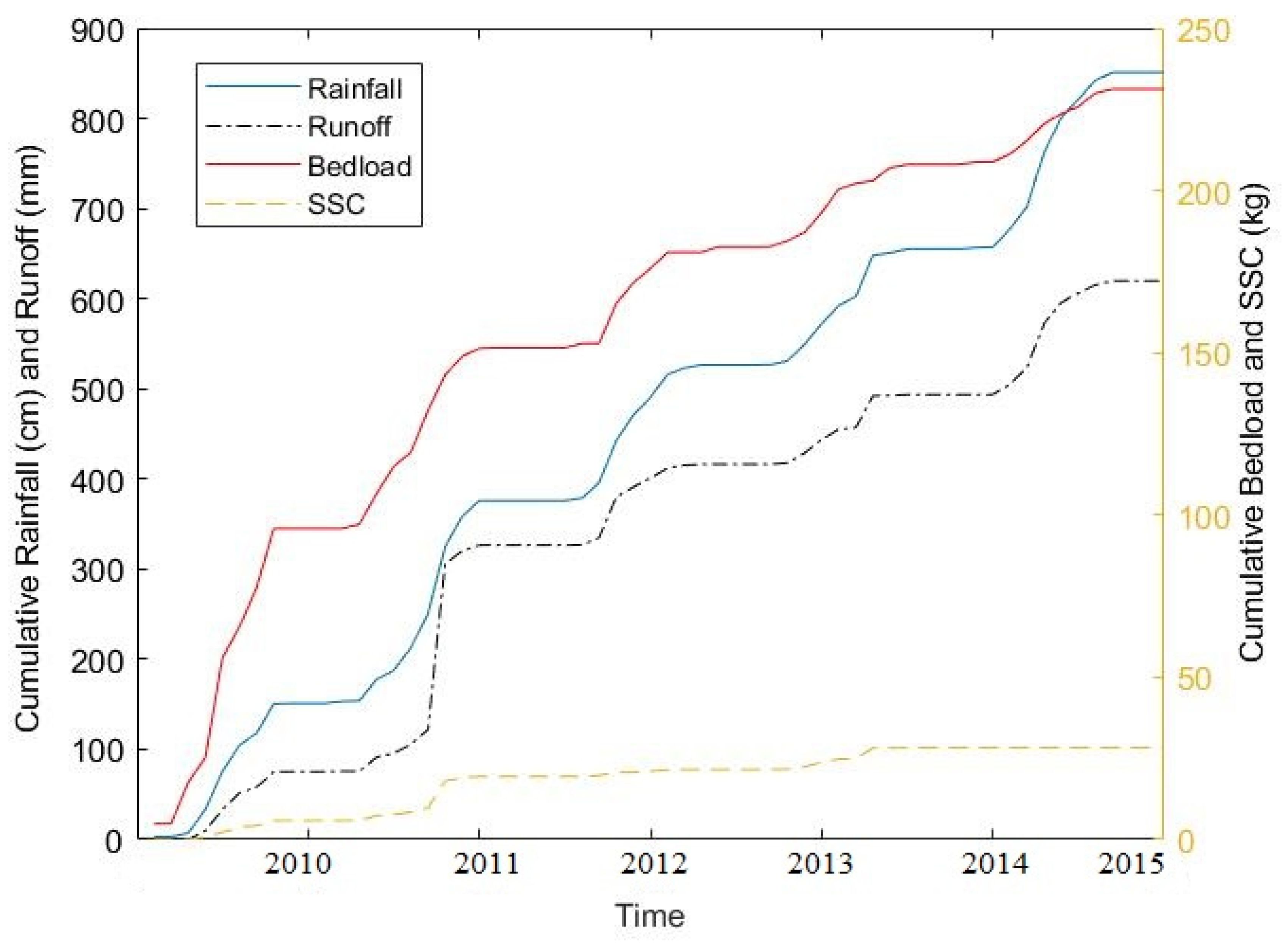
The annual rainfall, runoff and bedload over the five water years, as well as the annual suspended sediment load over the first four years (SSC was not measured in 2013–2014), are plotted in Figure 5. Corresponding to the high rainfall and runoff, both the bedload and suspended sediment load experienced high values in 2010–2011 (Figure 5). However, the bedload trend was dominated by an exponentially distributed decline, as previously shown by [44], with its peak in the first year, 2009–2010. Although 2013–2014 had the second-highest rainfall of the five years, it had the lowest bedload. Figure A3 (Appendix B) illustrates the seasonality of the events at the site and the dominance of the wet season for the mobilisation and transport of sediments. The annual totals were dominated by the seven-month wet season.
4.3. Bedload Controls
Over the 59 collection periods, the maximum bedload was 14.5 kg, which was collected on 6 January 2010, with accumulated rainfall and runoff depths of 357 mm and 18 mm, respectively. The minimum was 0.2 kg, collected on 28 May 2014, with cumulative rainfall and runoff depths of 41 mm and 1 mm, respectively. The bedload collection period of 31 January 2011–24 February 2011 contained extreme rainfall and runoff volumes of 666 mm and 180 mm, and a large but non-extreme bedload of 10.9 kg.
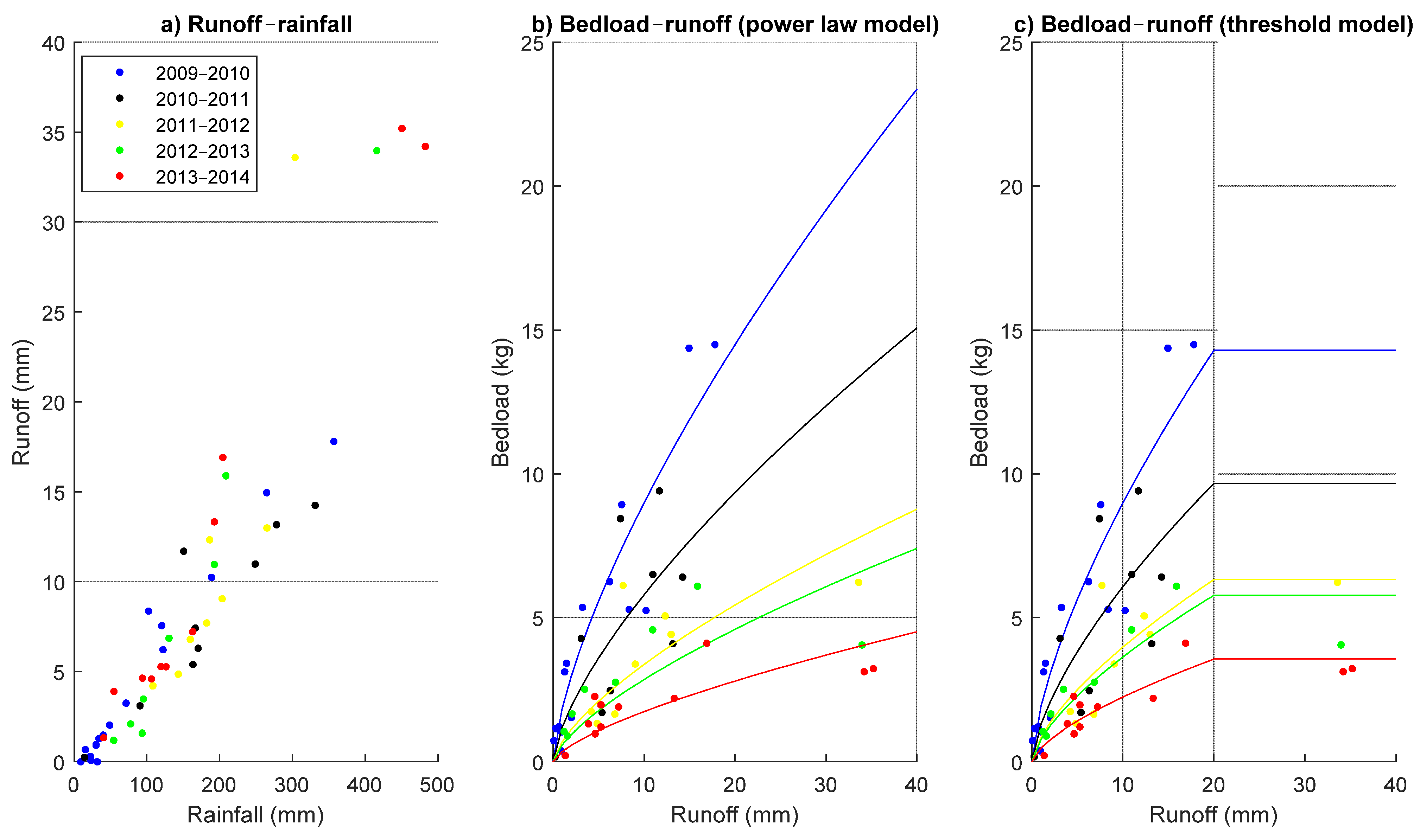
The relationship between the runoff and bedload data in Figure 6b is reasonably well represented by power-law functions fitted to the observations using least squares. The associated Nash–Sutcliffe efficiencies (NSEs, i.e., the proportion of the original bedload data variance explained by the function) were 0.86, 0.45, 0.43, 0.32 and 0.44 for the five measurement years (earliest to latest). The power parameter in these functions was set to 0.69, which worked reasonably well for all five years (if this parameter was optimised for each year individually, its values were 0.62, 0.88, 0.74, 0.53 and 0.69, the average of which is 0.69). The slope parameters were 1.83, 1.18, 0.69, 0.58 and 0.35 for the five measurement years (earliest to latest). The amount of bedload that could be delivered by a unit of runoff reduced each year, reflecting the exhaustion of the bedload shown in Figure 5. The power law fitted to the 2010–2011 observations in Figure 6b omitted the extreme event in the period 31 January 2011–24 February 2011, which had a much lower observed bedload (10.9 kg) than predicted by this model (42.5 kg). Furthermore, Figure 6b shows that the model also overestimated the bedload during the highest runoff periods in the three years subsequent to 2010–2011. This suggests that there may have been a threshold runoff rate beyond which the bedload rate increased relatively slowly or not at all. Figure 6c shows the result obtained when a threshold runoff parameter was added to the model, beyond which, the bedload remains constant. For this result, the power parameter was fixed at 0.67 (average of the five values optimised for each year individually) and the threshold fixed at 20 mm (an arbitrary value). In this case, the extreme event of 31 January 2011–24 February 2011 was included in the fitting, giving NSE values of 0.86, 0.60, 0.59, 0.77 and 0.77 for the five measurement years in turn, which is a considerable improvement on the previous model. The significance of this result is discussed later. For the bedload, the runoff ratios also tended to decrease within each year, with changes from the first to last measurement period in each year of −2.5, −0.1, −0.4, +0.2 and −0.1 kg/mm.
4.4. Turbidity Controls at the Event Scale
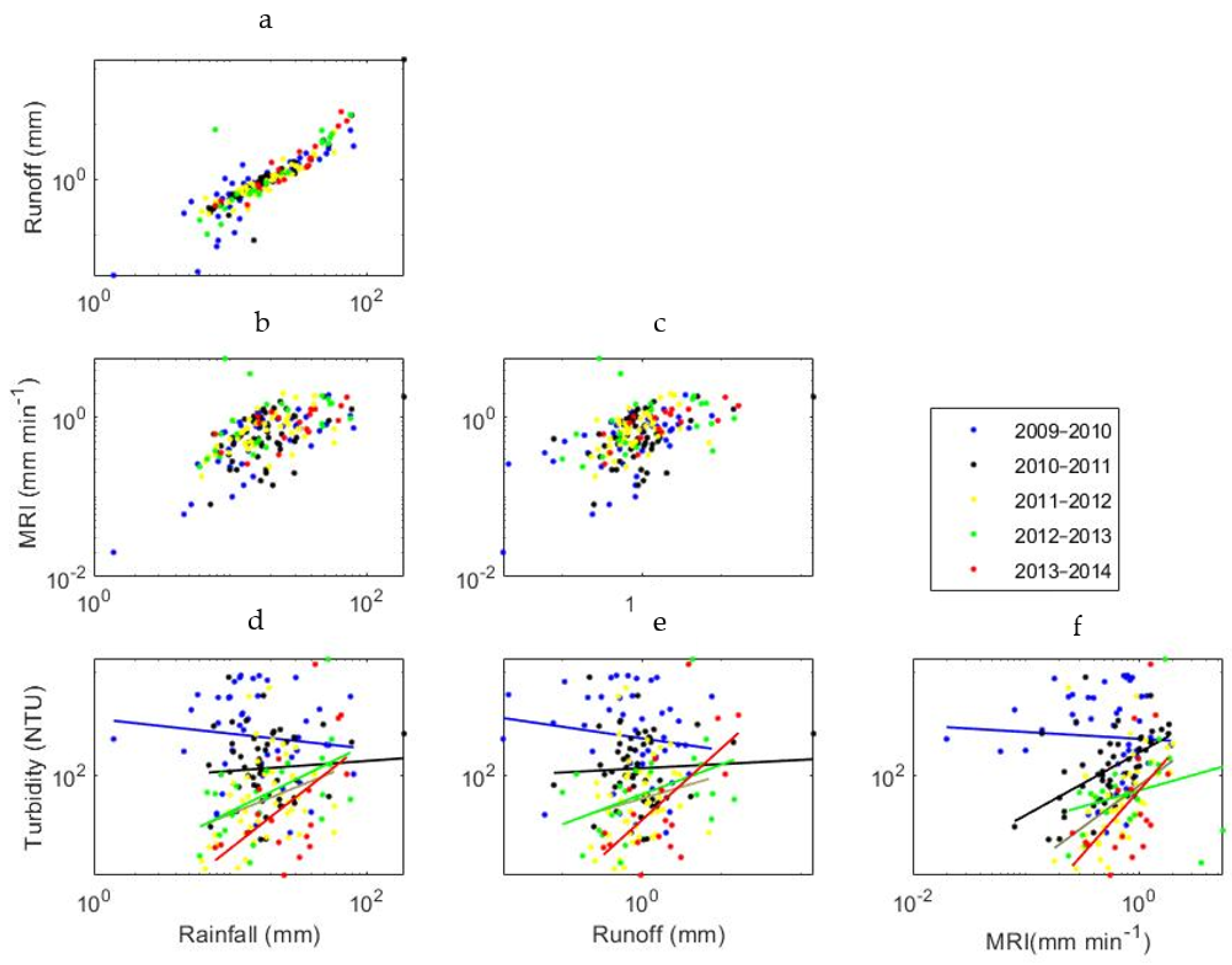
To study the event statistics and the response of the turbidity to storm events, 186 events with sufficiently complete turbidity (NTU) data were found. Table 1 summarises the statistics of these events and Figure 7 plots the selected variables. The average turbidity was most visibly related to the maximum rainfall intensity, as shown in Figure 7f, with evidence that the same maximum rainfall intensity caused larger NTU values in the earlier years (this was evident despite the highest NTU values not being recorded in the first year, as previously mentioned). The R2 and p-values obtained from regressing log10(turbidity) against log10(event rainfall), event runoff and maximum rainfall intensity (MRI) are shown in Table 1. The 2009–2010 data in each of Figure 7d–f had high levels of scattering, leading to the particularly low R2 values shown in Table 1, which were potentially partly associated with the change of the turbidity probe during that year. Over the other four years, the three variables together explained, on average, 34% of the variance of the log10(NTU) data (Table 1). It was difficult to isolate the individual effects because of the colinearity between the three explanatory variables; however, it is clear that both the intensities and rainfall volumes were relevant. Figure 7 indicates a general decrease in the event-averaged turbidity over time, with median values reducing from one year to the next, except in 2012–2013 (Table 1). However, the high variance of the turbidity data and the influence of outliers meant that the regression of the turbidity against the rainfall or runoff variables did not support the presence of trends in the suspended sediment mobility.
4.5. Turbidity Controls at the Intra-Event Scale
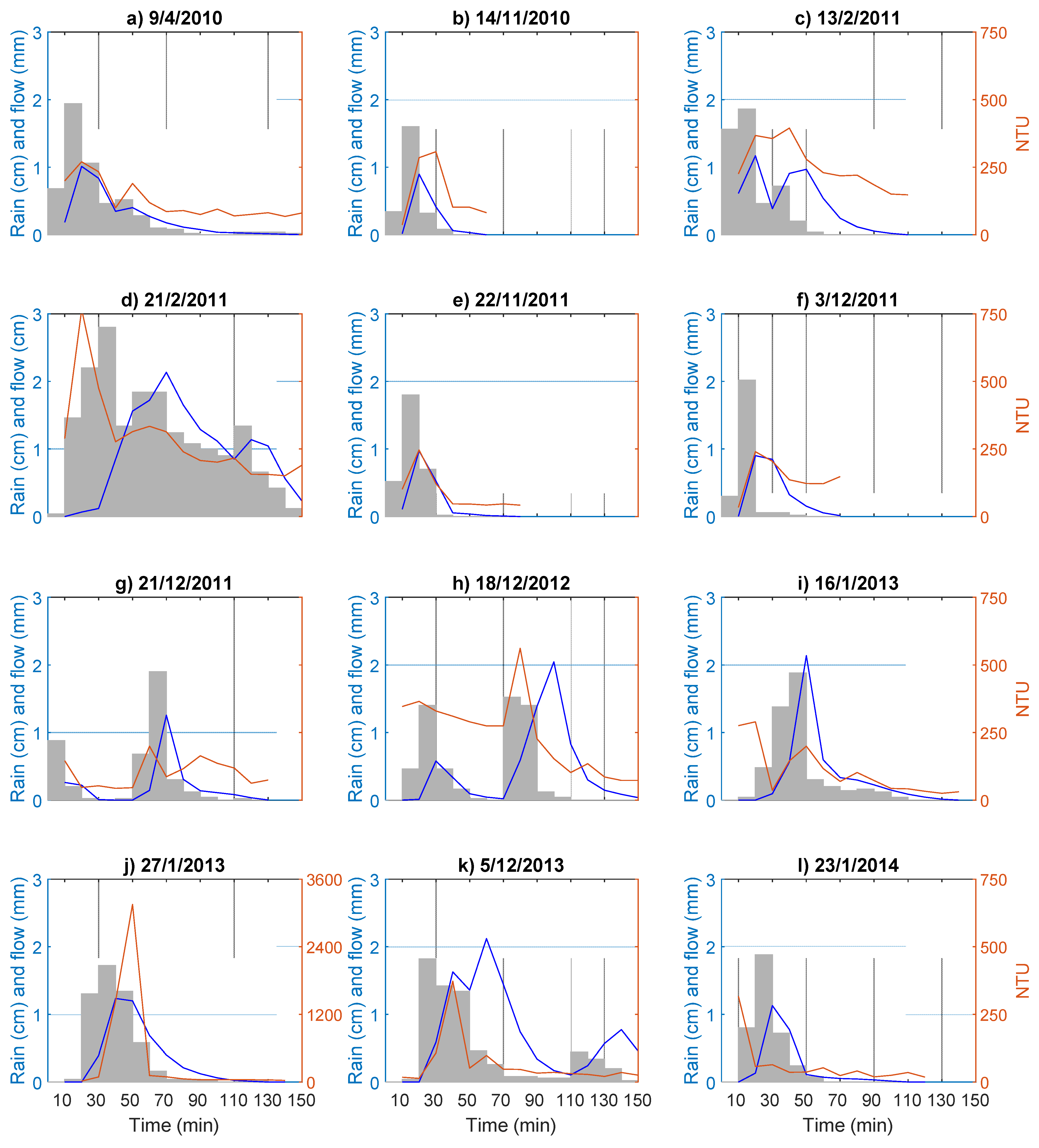
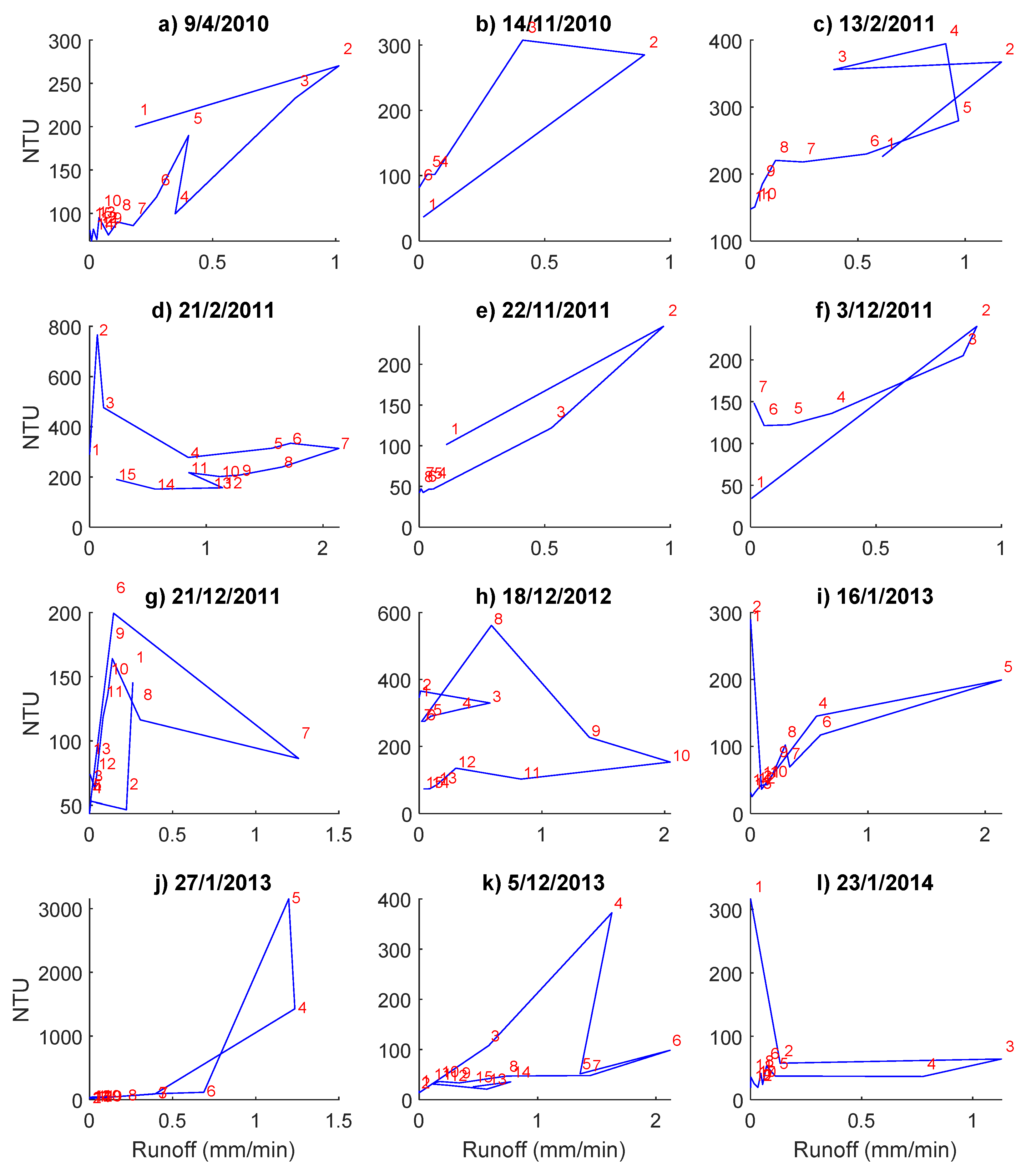
Figure 8 shows the typical event dynamics when using an exemplary set of 12 high-intensity events. These generally illustrate the expected runoff response, with the peak runoff lagging the peak rainfall by 0–20 min, typically 0–10 min. Figure 8 also illustrates the more random time differences between the peak NTU and the peak rainfall, and the peak NTU and the peak runoff. In three of the 12 examples (Figure 8d,i,l), the NTU distinctly peaked prior to any peak rainfall, indicating a flush of sediments near the start of the event. In four events (Figure 8a,e,f,h) the peak NTU was in the same 10-min interval as the peak rainfall, while in Figure 8b,c,j,k, the peak NTU was up to two 10-min intervals after the peak rainfall. The other event (Figure 8g) was the most complex, with an early peak NTU, a second peak NTU coinciding with the start of the main rainfall burst and a third peak NTU following the end of the rainfall burst. In six of the 12 examples (Figure 8d,g,h,i,k,l), the peak NTU occurred before the peak runoff, while in three, it coincided with the peak runoff (Figure 8a,e,f) and in three it followed the peak runoff (Figure 8b,c,j). Qualitative analysis of the runoff–turbidity hysteresis loops for the same 12 examples (Figure A4) indicated that seven were clockwise loops (Figure A4a,d,e,h,i,k,l), one was an anticlockwise loop (Figure A4b) and four were complex loops (Figure A4c,f,g,j). Both the hysteresis and the lag time analysis imply a characteristic dynamic of turbidity rise leading to a hydrograph rise, albeit with considerable variance and complexity.
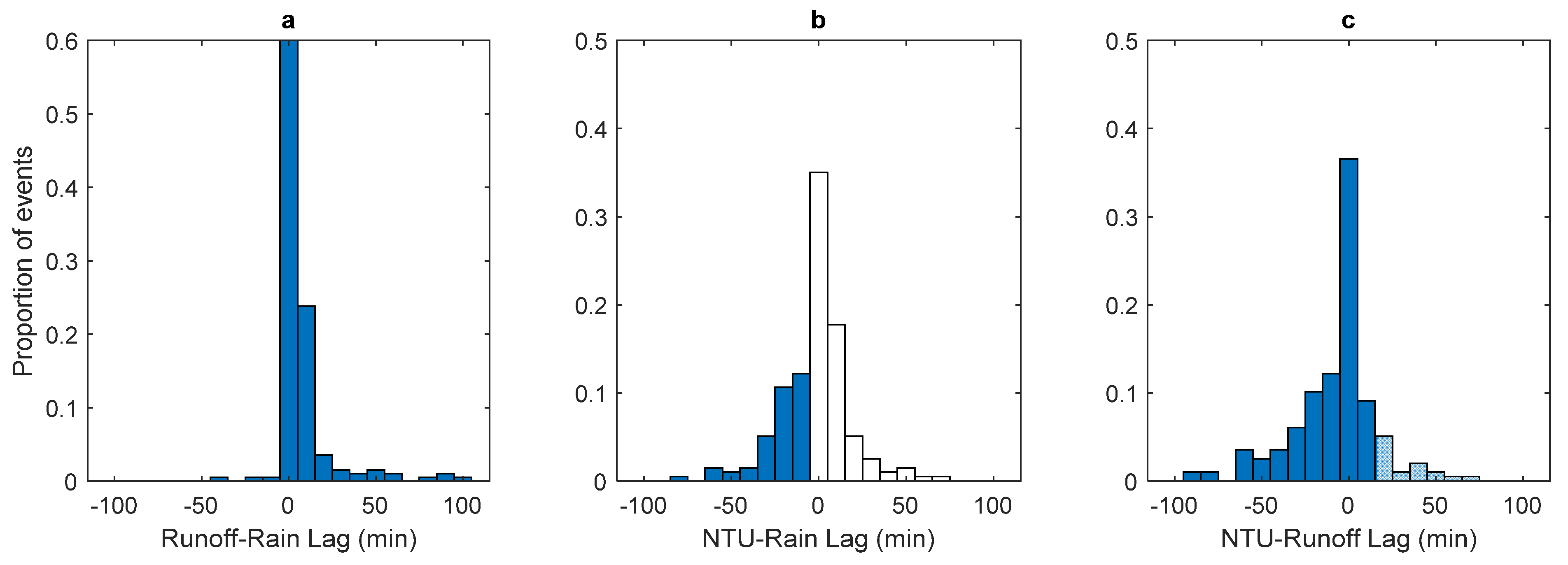
When including all 186 events, Figure 9 shows the distribution of lag times between the peak rainfall, peak runoff and peak NTU. Whether the peak rainfall preceded the peak NTU seemed to be random, with a near normal probability distribution, while the peak NTU occurred more often before than following a peak runoff. The highest and lowest values of lag were due to multipeak events.
5. Discussion
5.1. Sediment Loads
Figure 5 shows that 90% of the exported sediment mass over 2009–2013 was bedload (35% in 2009–2010 reducing to 11% in 2012–2013), supporting the findings of [55] showing that bedload is an important agent of geomorphic change. Figure 5 implies that the bedload trended towards a more constant annual value [56] and Figure 6 implies that the bedload–runoff ratio may have been stabilising. In 2009–2019, the total eroded mass of approximately 100 kg (Figure 5) was equivalent to a plot-average erosion rate of 44 mm/1000 years, and in 2012–2013, the eroded mass of approximately 30 kg was equivalent to 13 mm/1000 years, assuming a bulk density of 2500 kg m−3. This compares to erosion rates measured during 1981–1987 from nearby natural catchments of 16 mm/1000 years [57]. Although differences in rainfall, catchment size, slopes and other local features would need to be considered when interpreting the differences, these values indicate the potential significance of the observed stabilisation. The low erosion rates observed, relative to what may be expected for a disturbed landform exposed to intense rainfall, may be partly explained by the observed event runoff coefficients that were typically 5% (Figure 6a). These low runoff coefficients imply that the large proportion of rainfall was infiltrated rather than contributing to the stream power.
Figure 7 shows the differences in turbidity between years: out of the 55 events with turbidity higher than the average (192 NTU), 26 and 19 were in 2009–2010 and 2010–2011, respectively. This is assumed to be due to exhaustion of the available fine sediment, although increases in vegetation are also likely to have contributed to the stability [20,58]. Effects of hard-setting of the soil and the formation of biocrusts may have also contributed to a reduction in the mobilisation of the sediments from the surface [59,60,61,62].
As has been emphasised in many studies [61,63,64], a small period can be responsible for a large part of the sediment load. For example, 67% of the estimated suspended sediment load was associated with just 35% of the total runoff volume during the storm events of February 2011. However, for the bedload, the exhaustion effect dominated. While Figure 6 clearly demonstrates the important effect of the runoff on the bedload, it also shows that the bedload collection periods with the highest bedloads were concentrated in the first two years across a wide range of runoff volumes.
5.2. Relationship between the Rainfall–Runoff and Sediment Load
The climatic conditions at the investigated site were clearly different between the wet and dry seasons, with the onset of the wet season in October to November. The hydrological year starting in September is used as an ideal differentiator between periods of rainfall and periods of dry conditions, with the latter potentially influencing soil properties and soil consolidation.
Figure 6 provides some trends indicating that the bedload was related to the runoff volumes by a power law, potentially with a threshold, but that this relationship was non-stationary with the bedload exported for a given runoff volume declining over the years. This was presumably due to exhaustion of sediment from the surface from year to year, but also potentially due to surface properties becoming less susceptible to detachment of particles, for example, due to consolidation and/or vegetation growth. The fitted bedload–runoff relationships in Figure 6, although explaining much of the data variance (average NSE value for the models in Figure 6c was 0.72), all relationships had considerable residual errors. The residual errors may be associated with the intensity and other properties of the rainfall–runoff within the bedload collection periods that are not represented by the total runoff volume, as well as potential storage of bedload within the plot. The bedload accumulated during the extreme conditions of February 2011 and during other especially wet periods could be represented quite well by including a threshold runoff, beyond which, the bedload export did not increase (Figure 6c). However, the suggestion that a threshold exists remains speculative, and other models are possible. This cannot be investigated more thoroughly here due to the limited quantity and time resolution of the bedload rate measurements.
It has previously been observed that rainfall intensity is an important driver of fine sediment detachment [65]. In our study, only in 2010–2011 did the regression analysis clearly show the maximum rainfall intensity to have an effect on event-average turbidity over and above the effects of the rainfall and runoff volumes (Table 1). While the influence of the intensity is often difficult to discern in larger catchments due to spatial and temporal smoothing, in smaller catchments, its effect is more commonly seen and so would be expected at this plot scale [20,66,67]. In our case, the large amount of noise in the relationship between SSC and turbidity, as well as the potentially low contribution of fine sediment, are likely to be reasons why the rainfall intensity was not consistently seen to be statistically important.
5.3. Event Dynamics
In Figure 8 and Figure 9, the peak NTU more often preceded the peak runoff than followed it (6 events compared to 3 in Figure 8, 85 events compared to 40 in Figure 9). This accords with observations of flow–sediment hysteresis at small catchment scales [68], which is explained by the exhaustion of easily mobilised sediment in the rising hydrograph. The 40 events where the peak NTU followed the peak runoff might be explained by subplot-scale processes, for example, sediment being locally mobilised at various times through an event. The variability in detached particle sizes and their travel times associated with variability in rainfall, runoff energy and surface roughness of the rip lines [22,69] was also likely to have affected the variability of the lag times. The inter-event variability in the deposition and remobilisation within the plot, as well as in the travel times, are likely to depend on changes in the microtopography, the distribution of vegetation and the evolution in the rock properties, including their heterogeneity, all of which may be difficult to measure. The scale of the plot provides limited scope for these random effects to be integrated; hence, plots may have a higher variance in time lags compared to catchments. While the main effects of rainfall and plot-scale runoff on sediment amounts may be relatively straightforward to model deterministically, any attempt to simulate sediment dynamics may benefit from a stochastic representation of these more complex and less observable effects.
5.4. Limitations of the Analysis
Although a large number of samples (921) of SSCs were taken over the 4 years of the experiment, the absence of continuous SSC data meant that estimation of the suspended loads relied on the relationship between SSC and runoff, which changed over the years (Figure A1). There was considerable variance regarding these relationships such that they could only reasonably support estimation of seasonal and annual loads rather than inter- or intra-event SSC dynamics. Typically, turbidity is used to infill the SSC data; however, the relationship between SSC and turbidity (NTU) in this case (Figure A2), although reasonably consistent over the years, was considerably weaker than that between SSC and runoff.
Another limitation with respect to understanding bedload dynamics was the lack of bedload data for individual events; instead, it was available as an accumulated value over multiple events. Nevertheless, a total of 59 bedload samples were available over the 5 years, which is more than most bedload studies [70] and provided important insight into the predictability of bedload for this material.
5.5. Significance for Predictive Modelling
Erosion management planning in a mine rehabilitation context typically includes decisions about the combination of cover material, slopes, surface treatment (e.g., ripping or compaction) and vegetation planting and management whilst considering the local climate and other environmental factors. Experimental plots, such as that studied here, as well as the other plots on the Ranger Uranium Mine trial landform, are arguably essential resources for understanding the potential controls and their implications for management. Numerical modelling tools can be employed to guide decisions through interpolating and extrapolating the experimental data over time and to other potential designs, landform shapes and climate forcing. Requirements to predict the long-term performance of constructed landforms, such as those in mine rehabilitation, and the prediction of an acceptable certainty for landform stability into the future have to be based on measured data, empirical analysis and interpretations like those presented in this paper. Such information provides a basis for identifying appropriate predictive models for integration into the long-term predictive modelling of landform evolution.
6. Conclusions
This paper presents the results from analyses of a uniquely rich data set of runoff, bedload and suspended sediment loads from a constructed landform (mine waste rock dump) experimental plot in northern Australia. The data were analysed over annual, seasonal, event and subevent scales. The principal findings were as follows:
- The bedload exported from the plot was strongly and nonlinearly related to the runoff (and rainfall) volume, and the bedload per unit volume of runoff continually reduced over the five years.
- The nonlinear relationship between the suspended sediment concentration (as indicated by turbidity data) and runoff also changed over the years, with similar rainfall–runoff events in later years producing considerably lower turbidity.
These findings emphasise the need to consider nonstationarity in sediment mobilisation parameters when developing and applying erosion and landform evolution models as part of mine closure assessments. Another interesting observation was that the timing of the suspended sediments relative to rainfall and runoff appeared random from event to event, pointing to the importance of unobserved subplot scale processes and, consequently, the difficulty of deterministically modelling the erosion rates.
A reflection from the research is that plot-scale experimental studies provide important insights into sediment dynamics, and empirical analysis of their data provides a necessary basis for developing predictive models and improvement of existing landform evolution models. In the case study, longer-term experiments are recommended to support long-term landform stability studies.
Author Contributions
Conceptualization, S.Y.; Formal analysis, S.Y.; Methodology, S.Y.; Software, S.Y.; Supervision, N.M. and T.B. All authors have read and agreed to the published version of the manuscript.
Funding
This research received no external funding.
Institutional Review Board Statement
Not applicable.
Informed Consent Statement
Not applicable.
Data Availability Statement
Data sharing not applicable.
Acknowledgments
We pay our respects to all Traditional Owners of Kakadu National Park and the Darwin region where we conducted the research and monitoring and we acknowledge the Elders, past, present and emerging. We acknowledge the Supervising Scientist Branch (SSB) of the Australian Government, Department of Agriculture, Water and Environment, for supplying the data.
Conflicts of Interest
The authors declare no conflict of interest.
Appendix A. Infilling the Missing SSC Data
A total of 921 SSC observations were available from grab samples over a four-year period from 2009 to 2013. One of these, at 1.61 g/L, was considered to be suspiciously high relative to all other values and was removed.
Two possibilities for synthesising the continuous 10-min SSC data were considered: using a relationship between the turbidity (NTU) and SSC [71] and using a relationship between the runoff and SSC for each of the four years. A total of 225 of the 920 observations were within 1 min of a 1-min turbidity measurement. A scatter plot of these data (Figure A1) shows a significant but weak relationship (R2 = 0.03). This is consistent with the results from previous investigators [72,73]. Riley [72] suggested that various factors influence the SSC–turbidity relationship, including particle size variations, instrument stability, lighting conditions, organic load and biological activity on the probe. The relationship in Figure A1 was not considered suitable for synthesising the SSC data.
A stronger relationship between SSC and runoff exists (Figure A2), although it varies over the four years and there was a large degree of scatter (R2 = 0.21, 0.40, 0.07 and 0.24 for the four years). However, assuming unbiased and homogeneous errors in the relationships in Figure A2, synthesising the SSC series in this way allowed for the magnitudes of the annual SSC loads to be estimated and compared against annual bedloads. The relationships in Figure A2 were not fit for analysing inter-event and intra-event SSC dynamics, assuming that the errors would not average out at these short timescales. It would also limit the process insight gained from the analysis of the SSC dynamics if it was assumed that the suspended sediment was linearly related to runoff.
For the purpose of analysing the inter-event and intra-event suspended sediment dynamics, the untransformed 10-min NTU data were used. Since the purpose here was to analyse the differences between and within events, rather than produce absolute estimates of the suspended sediment loads, it was not necessary to convert into SSC units. However, it was necessary to assume that the NTU data gave a useful indication of changes in the suspended sediment concentrations over short timescales.
Figure A1.
Scatterplot relating the suspended sediment concentration (SSC) and the turbidity.

Figure A2.
Suspended sediment concentration relation with runoff for 2009–2010, 2010–2011, 2011–2012 and 2012–2013.
Figure A2.
Suspended sediment concentration relation with runoff for 2009–2010, 2010–2011, 2011–2012 and 2012–2013.

Appendix B. Illustrating the Seasonal Variability of Climate, Runoff and Suspended Sediments
Figure A3.
Cumulative monthly rainfall, runoff, bedload and suspended sediment.

Appendix C. Characterising the Runoff–NTU Hysteresis
Figure A4.
Runoff versus NTU hysteresis for 12 example events corresponding to Figure 8. The numbers in red show the time sequence of data points: (a) 9/04/2010, (b) 14/11/2010, (c) 13/2/2011, (d) 21/2/2011, (e) 22/11/2011, (f) 3/12/2011, (g) 21/12/2011, (h) 18/12/2012, (i) 16/1/2013, (j) 27/1/2012, (k) 5/12/2013 and (l) 23/1/2014.

References
- Riley, S.J. Aspects of the differences in the erodibility of the waste rock dump and natural surfaces, Ranger Uranium Mine, Northern Territory, Australia. Appl. Geogr. 1995, 15, 309–323. [Google Scholar] [CrossRef]
- Martín-Duque, J.F.; Zapico, I.; Oyarzun, R.; López García, J.A.; Cubas, P. A descriptive and quantitative approach regarding erosion and development of landforms on abandoned mine tailings: New insights and environmental implications from SE Spain. Geomorphology 2015, 239, 1–16. [Google Scholar] [CrossRef] [Green Version]
- Nyssen, J.; Vermeersch, D. Slope aspect affects geomorphic dynamics of coal mining spoil heaps in Belgium. Geomorphology 2010, 123, 109–121. [Google Scholar] [CrossRef] [Green Version]
- Martín-Moreno, C.; Martín-Duque, J.F.; Nicolau-Ibarra, J.M.; Hernando-Rodríguez, N.; Sanz-Santos, M.Á.; Sánchez-Castillo, L. Effects of topography and surface soil cover on erosion for mining reclamation: The experimental spoil heap at El Machorro Mine (Central Spain). Land Degrad. Dev. 2016, 27, 145–159. [Google Scholar] [CrossRef] [Green Version]
- Panagos, P.; Borrelli, P.; Meusburger, K.; Yu, B.; Klik, A.; Jae Lim, K.; Yang, J.; Ni, J.; Miao, C.; Chattopadhyay, N.; et al. Global rainfall erosivity assessment based on high-temporal resolution rainfall records. Sci. Rep. 2017, 7, 4175. [Google Scholar] [CrossRef] [Green Version]
- Guzman, C.D.; Tilahun, S.A.; Zegeye, A.D.; Steenhuis, T.S. Suspended sediment concentration-discharge relationships in the (sub-) humid Ethiopian highlands. Hydrol. Earth Syst. Sci. 2013, 17, 1067. [Google Scholar] [CrossRef] [Green Version]
- Thomas, S.; Ridd, P.V.; Day, G. Turbidity regimes over fringing coral reefs near a mining site at Lihir Island, Papua New Guinea. Mar. Pollut. Bull. 2003, 46, 1006–1014. [Google Scholar] [CrossRef]
- Alavinia, M.; Saleh, F.N.; Asadi, H. Effects of rainfall patterns on runoff and rainfall-induced erosion. Int. J. Sediment. Res. 2018, 34, 270–278. [Google Scholar] [CrossRef]
- Arjmand Sajjadi, S.; Mahmoodabadi, M. Sediment concentration and hydraulic characteristics of rain-induced overland flows in arid land soils. J. Soils Sediments 2015, 15, 710–721. [Google Scholar] [CrossRef]
- Walker, P.H.; Kinnell, P.I.A.; Green, P. Transport of a noncohesive sandy mixture in rainfall and runoff experiments. Soil Sci. Soc. Am. J. 1978, 42, 793–801. [Google Scholar] [CrossRef]
- Balacco, G. The interrill erosion for a sandy loam soil. Int. J. Sediment. Res. 2013, 28, 329–337. [Google Scholar] [CrossRef]
- Wang, Y.; You, W.; Fan, J.; Jin, M.; Wei, X.; Wang, Q. Effects of subsequent rainfall events with different intensities on runoff and erosion in coarse soil. Catena 2018, 170, 100–107. [Google Scholar] [CrossRef]
- Shen, H.; Zheng, F.; Wen, L.; Han, Y.; Hu, W. Impacts of rainfall intensity and slope gradient on rill erosion processes at loessial hillslope. Soil Till. Res. 2016, 155, 429–436. [Google Scholar] [CrossRef]
- Fang, N.-F.; Shi, Z.-H.; Li, L.; Guo, Z.-L.; Liu, Q.-J.; Ai, L. The effects of rainfall regimes and land use changes on runoff and soil loss in a small mountainous watershed. Catena 2012, 99, 1–8. [Google Scholar] [CrossRef]
- Peng, T.; Wang, S.-J. Effects of land use, land cover and rainfall regimes on the surface runoff and soil loss on karst slopes in southwest China. Catena 2012, 90, 53–62. [Google Scholar] [CrossRef]
- van Dijk, A.; Bruijnzeel, L.A.; Rosewell, C.J. Rainfall intensity-kinetic energy relationships: A critical literature appraisal. J. Hydrol. 2002, 261, 1–23. [Google Scholar] [CrossRef]
- Parsons, A.J.; Stone, P.M. Effects of intra-storm variations in rainfall intensity on interrill runoff and erosion. Catena 2006, 67, 68–78. [Google Scholar] [CrossRef]
- Flanagan, D.; Foster, G.; Moldenhauer, W. Storm pattern effect on infiltration, runoff, and erosion. Am. Soc. Agric. Biol. Eng. 1988, 31, 414–420. [Google Scholar] [CrossRef]
- Tao, W.; Wu, J.; Wang, Q. Mathematical model of sediment and solute transport along slope land in different rainfall pattern conditions. Sci. Rep. 2017, 7, 44082. [Google Scholar] [CrossRef]
- Zabaleta, A.; Martínez, M.; Uriarte, J.A.; Antigüedad, I. Factors controlling suspended sediment yield during runoff events in small headwater catchments of the Basque Country. Catena 2007, 71, 179–190. [Google Scholar] [CrossRef]
- Walker, P.; Hutka, J.; Moss, A.; Kinnell, P.I.A. Use of a versatile experimental system for soil erosion studies 1. Soil Sci. Soc. Am. J. 1977, 41, 610–612. [Google Scholar] [CrossRef]
- Saynor, M.J.; Lowry, J.B.C.; Boyden, J.M. Assessment of rip lines using CAESAR-Lisflood on a trial landform at the Ranger Uranium Mine. Land Degrad. Dev. 2019, 30, 504–514. [Google Scholar] [CrossRef]
- Gao, G.; Ma, Y.; Fu, B. Temporal Variations of flow–sediment relationships in a highly erodible catchment of the loess plateau, China. Land Degrad. Dev. 2016, 27, 758–772. [Google Scholar] [CrossRef] [Green Version]
- Zheng, M.; Yang, J.; Qi, D.; Sun, L.; Cai, Q. Flow–sediment relationship as functions of spatial and temporal scales in hilly areas of the Chinese Loess Plateau. Catena 2012, 98, 29–40. [Google Scholar] [CrossRef]
- Kiani-Harchegani, M.; Sadeghi, S.; Ghahramani, A. Intra-storm Variability of Coefficient of Variation of Runoff and Soil Loss in Consecutive Storms at Experimental Plot Scale. In Climate Change Impacts on Hydrological Processes and Sediment Dynamics: Measurement, Modelling and Management; Springer: Berlin, Germany, 2019; pp. 98–103. [Google Scholar]
- Anache, J.A.A.; Wendland, E.C.; Oliveira, P.T.S.; Flanagan, D.C.; Nearing, M.A. Runoff and soil erosion plot-scale studies under natural rainfall: A meta-analysis of the Brazilian experience. Catena 2017, 152, 29–39. [Google Scholar] [CrossRef]
- Sadeghi, S.H.R.; Seghaleh, M.B.; Rangavar, A.S. Plot sizes dependency of runoff and sediment yield estimates from a small watershed. Catena 2013, 102, 55–61. [Google Scholar] [CrossRef]
- Liu, Y.; Fu, B.; Lü, Y.; Wang, Z.; Gao, G. Hydrological responses and soil erosion potential of abandoned cropland in the Loess Plateau, China. Geomorphology 2012, 138, 404–414. [Google Scholar] [CrossRef]
- Cerdan, O.; Govers, G.; Le Bissonnais, Y.; Van Oost, K.; Poesen, J.; Saby, N.; Gobin, A.; Vacca, A.; Quinton, J.; Auerswald, K.; et al. Rates and spatial variations of soil erosion in Europe: A study based on erosion plot data. Geomorphology 2010, 122, 167–177. [Google Scholar] [CrossRef]
- Fu, B.; Zhao, W.; Chen, L.; Zhang, Q.; Lü, Y.; Gulinck, H. Assessment of soil erosion at large watershed scale using RUSLE and GIS: A case study in the Loess Plateau of China. Land Degrad. Dev. 2005, 16, 73–85. [Google Scholar] [CrossRef]
- Jetten, V.; De Roo, A.; Favis-Mortlock, D.J.C. Evaluation of field-scale and catchment-scale soil erosion models. Catena 1999, 37, 521–541. [Google Scholar] [CrossRef]
- Bagarello, V.; Ferro, V. Plot-scale measurement of soil erosion at the experimental area of Sparacia (southern Italy). Hydrol. Process. 2004, 18, 141–157. [Google Scholar] [CrossRef]
- Shit, P.K.; Bhunia, G.S.; Maiti, R. Science, E. Effect of vegetation cover on sediment yield: An empirical study through plots experiment. Environ. Earth Sci. 2012, 2, 32–40. [Google Scholar]
- Moreno-de las Heras, M.; Nicolau, J.M.; Merino-Martín, L.; Wilcox, B.P. Plot-scale effects on runoff and erosion along a slope degradation gradient. Water Resour. Res. 2010, 46, 12. [Google Scholar] [CrossRef] [Green Version]
- Boix-Fayos, C.; Martínez-Mena, M.; Arnau-Rosalén, E.; Calvo-Cases, A.; Castillo, V.; Albaladejo, J. Measuring soil erosion by field plots: Understanding the sources of variation. Earth Sci. Rev. 2006, 78, 267–285. [Google Scholar] [CrossRef]
- Godone, D.; Stanchi, S. Research on Soil Erosion; InTech Open: London, UK, 2012. [Google Scholar] [CrossRef] [Green Version]
- Chaplot, V.; Le Bissonnais, Y. Field measurements of interrill erosion under different slopes and plot sizes. Earth Surf. Process. Landf. 2000, 25, 145–153. [Google Scholar] [CrossRef]
- Hu, J.; Zhao, G.; Mu, X.; Hörmann, G.; Tian, P.; Gao, P.; Sun, W. Effect of soil and water conservation measures on regime-based suspended sediment load during floods. Sustain. Cities Soc. 2020, 55, 102044. [Google Scholar] [CrossRef]
- Sadeghi, S.H.; Moosavi, V.; Karami, A.; Behnia, N. Soil erosion assessment and prioritization of affecting factors at plot scale using the Taguchi method. J. Hydrol. 2012, 448-449, 174–180. [Google Scholar] [CrossRef]
- Temple, P.H. Measurements of runoff and soil erosion at an erosion plot scale with particular reference to Tanzania. Geogr. Ann. Ser. A Phys. Geogr. 1972, 54, 203–220. [Google Scholar] [CrossRef]
- Lowry, J.B.C.; Narayan, M.; Hancock, G.R.; Evans, K.G. Understanding post-mining landforms: Utilising pre-mine geomorphology to improve rehabilitation outcomes. Geomorphology 2019, 328, 93–107. [Google Scholar] [CrossRef]
- Festin, E.S.; Tigabu, M.; Chileshe, M.N.; Syampungani, S.; Odén, P.C. Progresses in restoration of post-mining landscape in Africa. J. For. Res. 2019, 30, 381–396. [Google Scholar] [CrossRef] [Green Version]
- Saynor, M.J.; Lowry, J.; Erskine, W.D.; Coulthard, T.; Hancock, G.; Jones, D.; Lu, P. Assessing erosion and run-off performance of a trial rehabilitated mining landform. In Proceedings of the Life of Mine Conference, Brisbane, QLD, Australia, 10–12 July 2012; pp. 10–12. [Google Scholar]
- Saynor, M.J.; Erskine, W.D. Bed load losses from experimental plots on a rehabilitated uranium mine in northern Australia. In Proceedings of the Life of Mine Conference, Brisbane, QLD, Australia, 28–30 September 2016. [Google Scholar]
- Zhang, L.-T.; Gao, Z.-L.; Yang, S.-W.; Li, Y.-H.; Tian, H.-W. Dynamic processes of soil erosion by runoff on engineered landforms derived from expressway construction: A case study of typical steep spoil heap. Catena 2015, 128, 108–121. [Google Scholar] [CrossRef]
- Verbist, B.; Poesen, J.; van Noordwijk, M.; Widianto; Suprayogo, D.; Agus, F.; Deckers, J. Factors affecting soil loss at plot scale and sediment yield at catchment scale in a tropical volcanic agroforestry landscape. Catena 2010, 80, 34–46. [Google Scholar] [CrossRef]
- Hancock, G.R.; Evans, K.G.; Willgoose, G.R.; Moliere, D.R.; Saynor, M.J.; Loch, R.J. Medium-term erosion simulation of an abandoned mine site using the SIBERIA landscape evolution model. Soil Res. 2000, 38, 249–264. [Google Scholar] [CrossRef]
- Lacy, H. Mine landforms in Western Australia from dump to landform design: Review, reflect and a future direction. In Proceedings of the 13th International Conference on Mine Closure, Perth, Australia, 3–5 September 2019; pp. 371–384. [Google Scholar]
- Hancock, G.R.; Grabham, M.K.; Martin, P.; Evans, K.G.; Bollhöfer, A. A methodology for the assessment of rehabilitation success of post mining landscapes—sediment and radionuclide transport at the former Nabarlek uranium mine, Northern Territory, Australia. Sci. Total. Environ. 2006, 354, 103–119. [Google Scholar] [CrossRef]
- Australian Government. Environmental Requirements of the Commonwealth of Australia for the Operation of Ranger Uranium Mine. 1999; p. 1e11. Available online: https://www.environment.gov.au/science/supervising-scientist/publications/environmentalrequirements-ranger-uranium-mine (accessed on 22 June 2020).
- Hancock, G.; Saynor, M.; Lowry, J.; Erskine, W. How to account for particle size effects in a landscape evolution model when there is a wide range of particle sizes. Environ. Model. Softw. 2020, 124, 104582. [Google Scholar] [CrossRef]
- ERA. Unique Reference: 1400 Ranger Mine Closure Plan; Australian Government, Department of the Environment and Energy: Darwin, Australia, 2018. [Google Scholar]
- Li, G.-L.; Zheng, T.H.; Fu, Y.; Li, B.Q.; Zhang, T. Soil detachment and transport under the combined action of rainfall and runoff energy on shallow overland flow. J. Mt. Sci. 2017, 14, 1373–1383. [Google Scholar] [CrossRef]
- Chen, J.; Chang, H. Dynamics of wet-season turbidity in relation to precipitation, discharge, and land cover in three urbanizing watersheds, Oregon. River Res. Appl. 2019, 35, 892–904. [Google Scholar] [CrossRef]
- Schneider, J.M.; Turowski, J.M.; Rickenmann, D.; Hegglin, R.; Arrigo, S.; Mao, L.; Kirchner, J.W. Scaling relationships between bed load volumes, transport distances, and stream power in steep mountain channels. Geophys. Res. Earth Surf. 2014, 119, 533–549. [Google Scholar] [CrossRef]
- Saynor, M.; Lowry, J.; Boyden, J. The impact of rip lines on erosion at the Ranger mine site. In Proceedings of the Life of Mine Conference 2018, Brisbane, QLD, Australia, 25–27 July 2018; pp. 150–154. [Google Scholar]
- Duggan, K. Erosion and sediment yields in the Kakadu region of northern Australia. Stream Eros. Sediment. Transp. 1994, 224, 373384. [Google Scholar]
- Wei, W.; Chen, L.; Fu, B.; Huang, Z.; Wu, D.; Gui, L. The effect of land uses and rainfall regimes on runoff and soil erosion in the semi-arid loess hilly area, China. J. Hydrol. 2007, 335, 247–258. [Google Scholar] [CrossRef]
- So, H. Sealing, crusting and hardsetting soils: Productivity and conservation. In Proceedings of the second International Symosium on Sealing, Crusting and Hardsetting Soils: Productivity and Conservation held at the University of Queensland, Brisbane, QLD, Australia, 7–11 February 1994. [Google Scholar]
- Blackwell, P.S. Slaking and hard setting soils: Some research and management aspects. Soil Till. Res. 1992, 25, 111–261. [Google Scholar] [CrossRef]
- Mohamadi, M.A.; Kavian, A. Effects of rainfall patterns on runoff and soil erosion in field plots. Int. Soil Water Conserv. Res. 2015, 3, 273–281. [Google Scholar] [CrossRef] [Green Version]
- Kidron, G.J.; Xiao, B.; Benenson, I. Data variability or paradigm shift. Slow versus fast recovery of biological soil crusts-a review. Sci. Total Environ. 2020, 721, 137683. [Google Scholar] [CrossRef]
- Gonzalez-Hidalgo, J.C.; Batalla, R.J.; Cerda, A.; de Luis, M. A regional analysis of the effects of largest events on soil erosion. Catena 2012, 95, 8–590. [Google Scholar] [CrossRef]
- Wei, W.; Chen, L.; Fu, B.; Lü, Y.; Gong, J.J.H.P.A.I.J. Responses of water erosion to rainfall extremes and vegetation types in a loess semiarid hilly area, NW China. Hydrol. Process. 2009, 23, 1780–1791. [Google Scholar] [CrossRef]
- Miura, S.; Hirai, K.; Yamada, T. Transport rates of surface materials on steep forested slopes induced by raindrop splash erosion. J. For. Res. 2002, 7, 201–211. [Google Scholar] [CrossRef]
- Oeurng, C.; Sauvage, S.; Sánchez-Pérez, J.-M. Dynamics of suspended sediment transport and yield in a large agricultural catchment, southwest France. Earth Surf. Process. Landf. 2010, 35, 1289–1301. [Google Scholar] [CrossRef] [Green Version]
- Shen, C.; Liao, Q.; Titi, H.H.; Li, J. Turbidity of stormwater runoff from highway construction sites. Environ. Eng. 2018, 144, 04018061. [Google Scholar] [CrossRef]
- Moliere, D.R.; Evans, K.G.; Saynor, M.J.; Erskine, W.D. Estimation of suspended sediment loads in a seasonal stream in the wet-dry tropics, Northern Territory, Australia. Hydrol. Process. 2004, 18, 531–544. [Google Scholar] [CrossRef]
- Solano-Rivera, V.; Geris, J.; Granados-Bolaños, S.; Brenes-Cambronero, L.; Artavia-Rodríguez, G.; Sánchez-Murillo, R.; Birkel, C. Exploring extreme rainfall impacts on flow and turbidity dynamics in a steep, pristine and tropical volcanic catchment. Catena 2019, 182, 104118. [Google Scholar] [CrossRef]
- Kheirfam, H.; Sadeghi, S.H. Variability of bed load components in different hydrological conditions. J. Hydrol. Reg. Stud. 2017, 10, 145–156. [Google Scholar] [CrossRef]
- Lewis, J. Turbidity-controlled sampling for suspended sediment load estimation. Technological and Methodological Advances. In Proceedings of the Oslo Workshop; Bogen, J., Fergus, T., Walling, D.E., Eds.; IAHS Press: Wallingford, CT, USA, 2003; pp. 13–20. [Google Scholar]
- Riley, S.J. The sediment concentration–turbidity relation: Its value in monitoring at Ranger Uranium Mine, Northern Territory, Australia. Catena 1998, 32, 1–14. [Google Scholar] [CrossRef]
- Moliere, D.; Saynor, M.; Evans, K. Suspended sediment concentration-turbidity relationships for Ngarradj–a seasonal stream in the wet-dry tropics. Australas. J. Water Resour. 2005, 9, 37–48. [Google Scholar] [CrossRef]
Figure 1.
Location plan and plot topography: (A) the location of the landform within the Ranger Uranium Mine, (B) the location of plot 1 within the landform and (C) the digital elevation model (DEM) of plot 1. PVC: polyvinyl chloride.
Figure 1.
Location plan and plot topography: (A) the location of the landform within the Ranger Uranium Mine, (B) the location of plot 1 within the landform and (C) the digital elevation model (DEM) of plot 1. PVC: polyvinyl chloride.

Figure 2.
Grain size distribution for the trial landform [51].
Figure 2.
Grain size distribution for the trial landform [51].

Figure 3.
Runoff and turbidity measurement setup [43].
Figure 3.
Runoff and turbidity measurement setup [43].

Figure 4.
(a) Rainfall intensity histogram, (b) rainfall time series, (c) cumulative rainfall for each year (Month 1 is September), (d) runoff intensity histogram, (e) runoff time series and (f) cumulative runoff for each year (Month 1 is September).
Figure 4.
(a) Rainfall intensity histogram, (b) rainfall time series, (c) cumulative rainfall for each year (Month 1 is September), (d) runoff intensity histogram, (e) runoff time series and (f) cumulative runoff for each year (Month 1 is September).

Figure 5.
Annual distribution of the rainfall, runoff, bedload and suspended sediment load (SSload).
Figure 5.
Annual distribution of the rainfall, runoff, bedload and suspended sediment load (SSload).

Figure 6.
Relationships between the (a) runoff and rainfall volumes in the bedload collection periods, (b) bedload export and runoff volumes in the bedload collection periods with a fitted power-law model and (c) bedload export and runoff volumes in the bedload collection periods with a fitted power-law and threshold model. The data points for the period of 31 January 2011–24 February 2011 (rainfall = 666 mm, runoff = 180 mm, bedload = 10.9 kg) were omitted from all plots to assist with presentation clarity. The power-law model in (b) omitted this point from the model fitting, while the power law with the threshold model in (c) included this point in the model fitting.

Figure 7.
Scatterplots showing data from 186 events: (a) rainfall vs. runoff, (b) rainfall vs. MRI (maximum rainfall intensity during an event), (c) runoff vs. MRI, (d) rainfall vs. runoff-weighted turbidity, (e) runoff vs. runoff-weighted turbidity and (f) MRI vs. runoff-weighted turbidity. The associated R2 and p-values are listed in Table 1.

Figure 8.
Rainfall–runoff–turbidity dynamics for the 12 largest events in terms of the rainfall volumes with complete turbidity data. The grey bars represent rainfall (cm per 10 min interval), the blue lines signify the runoff (mm per 10 min interval) and the brown lines represent the turbidity (NTU). A common x-axis scale of 0 to 150 min was used to ease the comparison, although some events ceased prior to 150 min. A common y-axis scale of 0 to 750 NTU was used, except for (j), which has a greater NTU range. The runoff in (d) was exceptionally large and thus it is presented in units of centimetres instead of millimetres.

Figure 9.
Lag time histograms: (a) time to peak runoff minus time to peak rainfall; (b) time to peak NTU minus time to peak rainfall; (c) time to peak NTU minus time to peak runoff.
Figure 9.
Lag time histograms: (a) time to peak runoff minus time to peak rainfall; (b) time to peak NTU minus time to peak rainfall; (c) time to peak NTU minus time to peak runoff.


Table 1.
Statistical values for the observed 186 rainfall events in the five water years from 2009 to 2014.
Table 1.
Statistical values for the observed 186 rainfall events in the five water years from 2009 to 2014.
| Statistic | 2009–2010 | 2010–2011 | 2011–2012 | 2012–2013 | 2013–2014 |
|---|---|---|---|---|---|
| Number of events with sufficient nephelometric turbidity units (NTU) data | 44 | 53 | 44 | 24 | 18 |
| Runoff coefficient—mean (standard deviation) over events | 0.05 (0.02) | 0.06 (0.09) | 0.05 (0.01) | 0.08 (0.1) | 0.06 (0.04) |
| Event duration—mean (standard deviation) over events (min) | 162 (206) | 126 (104) | 110 (99) | 111 (119) | 165 (113) |
| Rainfall volume mean (standard deviation) (mm) | 21.3 (17.7) | 22.7 (26.2) | 20.6 (12.2) | 26.1 (20.2) | 32.2 (19.1) |
| Runoff volume mean (standard deviation) (mm) | 1.2 (1.7) | 3.9 (18.5) | 1.1 (1.1) | 2.7 (3.1) | 3.3 (3.6) |
| Maximum rainfall intensity (MRI) mean (standard deviation) over events (mm 10 min−1) | 0.64 (0.38) | 0.69 (0.42) | 0.78 (0.42) | 1.17 (1.2) | 0.9 (0.4) |
| Runoff weighted turbidity—mean (standard deviation) over events (NTU) | 351 (282) | 159 (146) | 95 (133) | 127 (257) | 143 (279) |
| Runoff weighted turbidity—median over events (NTU) | 252 | 109 | 53 | 66 | 34 |
| R2 (p-value) by regressing log10(NTU) against log10(rainfall) | 0.02 (0.6) | 0.006 (0.9) | 0.20 (0.04) | 0.28 (0.04) | 0.41 (0.02) |
| R2 (p-value) by regressing log10(NTU) against log10(runoff) | 0.02 (0.3) | 0.003 (0.7) | 0.03 (0.04) | 0.19 (0.04) | 0.39 (0.006) |
| R2 (p-value) by regressing log10(NTU) against log10(MRI) | 0.004 (0.7) | 0.27 (0.0001) | 0.22 (0.001) | 0.07 (0.23) | 0.26 (0.03) |
| R2 (p-value) by regressing log10(NTU) against log10(rainfall), log10(runoff) and log10(MRI) | 0.02 (0.6) | 0.31 (0.0001) | 0.34 (0.005) | 0.28 (0.1) | 0.41 (0.02) |
Publisher’s Note: MDPI stays neutral with regard to jurisdictional claims in published maps and institutional affiliations. |
© 2021 by the authors. Licensee MDPI, Basel, Switzerland. This article is an open access article distributed under the terms and conditions of the Creative Commons Attribution (CC BY) license (https://creativecommons.org/licenses/by/4.0/).
Share and Cite
MDPI and ACS Style
Yavari, S.; McIntyre, N.; Baumgartl, T. An Empirical Analysis of Sediment Export Dynamics from a Constructed Landform in the Wet Tropics. Water 2021, 13, 1087. https://doi.org/10.3390/w13081087
AMA Style
Yavari S, McIntyre N, Baumgartl T. An Empirical Analysis of Sediment Export Dynamics from a Constructed Landform in the Wet Tropics. Water. 2021; 13(8):1087. https://doi.org/10.3390/w13081087
Chicago/Turabian StyleYavari, Shahla, Neil McIntyre, and Thomas Baumgartl. 2021. "An Empirical Analysis of Sediment Export Dynamics from a Constructed Landform in the Wet Tropics" Water 13, no. 8: 1087. https://doi.org/10.3390/w13081087
Note that from the first issue of 2016, this journal uses article numbers instead of page numbers. See further details here.