
Using the General Regression Neural Network Method to Calibrate the Parameters of a Sub-Catchment


1
Department of Civil Engineering, National Taipei University of Technology, Taipei 10608, Taiwan
2
Department of Civil Engineering, Ningde Normal University, Ningde 352100, China
*
Author to whom correspondence should be addressed.
Water 2021, 13(8), 1089; https://doi.org/10.3390/w13081089
Submission received: 12 March 2021
/
Revised: 5 April 2021
/
Accepted: 12 April 2021
/
Published: 15 April 2021
Abstract
:Computer software is an effective tool for simulating urban rainfall–runoff. In hydrological analyses, the storm water management model (SWMM) is widely used throughout the world. However, this model is ineffective for parameter calibration and verification owing to the complexity associated with monitoring data onsite. In the present study, the general regression neural network (GRNN) is used to predict the parameters of the catchment directly, which cannot be achieved using SWMM. Then, the runoff curve is simulated using SWMM, employing predicted parameters based on actual rainfall events. Finally, the simulated and observed runoff curves are compared. The results demonstrate that using GRNN to predict parameters is helpful for achieving simulation results with high accuracy. Thus, combining GRNN and SWMM creates an effective tool for rainfall–runoff simulation.
1. Introduction
Urbanization has resulted in land use changes that include increased amounts of impervious pavement in cities. This has affected the original water cycle in such cities by increasing urban surface runoff volume, the confluence time of urban flooding, and water pollution [1,2,3], which have led to significant human and economic casualties. In the past few years, many scholars have focused on restoring the urban water cycle, which consists of rain and floodwater in cities [4,5,6,7]. Numerical hydrologic modeling is a primary tool for designing site drainage plans and assessing their potential improvement over the original conditions. Many numerical hydrologic models are available, including the storm water management model (SWMM), soil and water assessment tool (SWAT), the Hydrologic Engineering Center’s river analysis system (HEC-RAS), variable infiltration capacity model, identification of unit hydrographs and component flows from rainfall (IHACRES), and satellite-based hydrological model (SHM) [8,9,10,11,12,13,14]. Among them, SWMM is the most widely used worldwide for urban watershed hydrology and water quality modeling [15]. Additionally, SWMM contains a flexible set of hydraulic modeling capabilities that enables it to account for hydrologic processes, estimate the production of pollutant loads, and evaluate the performance of green infrastructure under single-event or long-term precipitation. In particular, SWMM is widely adopted in Taiwan for hydrological research owing to its high potentiality [16,17,18,19].
Under the concept of a sponge city, the effect of runoff regulation has recently become an important indicator in Taiwan. Rainfall is considered to be the primary source of surface runoff, which can be controlled to meet human requirements. To better understand the relationship between rainfall and runoff, SWMM is often used in the analysis of urban runoff [16,17,18,19,20]. However, simulation with SWMM requires the determination of numerous field parameters to match the actual conditions of the experiment site. Moreover, it is difficult to obtain a sufficient amount of detailed information on some parameters to determine their actual value. As a consequence, model calibration is required before investigating the relationship between rainfall and runoff to make the corresponding model-computed predictions (e.g., runoff) as close as possible to the field-measured observations for the same rain event [20,21,22].
Alternatively, a traditional parameter calibration method needs to adjust the parameters in SWMM many times until the output and observation results are similar. However, this procedure relies on the rich experience of a practitioner to evaluate the most suitable parameter values. This matter warrants serious consideration. The phenomenon of “different parameters but same result” occurs easily in practical applications, as reported in the literature [23,24,25]. For example, Beven and Freer suggested that an optimal model is needed [23]; that is, research on the workable model structure should be conducted to avoid this phenomenon and to pursue higher calibration efficiency and accuracy. For this purpose, some scholars have attempted to calibrate the parameters from an external programming environment by selecting logical algorithms based on the characteristics of the software and its calibration parameters. This method has proved to be effective, particularly when using neural network algorithms to calibrate the parameters in the hydrology field [26,27,28,29,30].
Many neural network algorithms have been developed for various applications. Artificial neural network (ANN)-based rainfall–runoff models have been widely recommended. In 1943, McCulloch and Pitts proposed the first ANN, and Rosenblatt and several other researchers developed a class of neural networks in the late 1950s known as a perceptron network. However, the perceptron network was inherently limited until the 1980s. Although many limitations have been reported in neural network applications in the past few decades, the development of computers in the past two decades has improved their performance. Recently, an ANN known as the general regression neural network (GRNN) has shown promise owing to its rapid calculation speed and good nonlinear approximation performance [28,29]. Therefore, it is widely used in many academic fields, including hydrology [31,32,33,34]. Apaydin et al. [31] simulated the daily streamflow to the Ermenek hydroelectric dam reservoir using deep recurrent neural network architectures and reported highly accurate results. Turan and Yurdusev [32] used GRNN to estimate unmeasured data using the data of the four runoff gauge stations on the Birs river in Switzerland. They indicated that GRNN is capable of yielding satisfactory outputs. Other scholars have reported similar results [33,34]. However, the previous studies focus mostly on the application of runoff forecasting by GRNN without considering its combination with hydrological modeling software such as SWMM. Although SWMM has limitations when it comes to parameter calibration, GRNN is expected to compensate for this deficiency. Hence, the present study focuses on parameter optimization combining GRNN and SWMM.
In particular, we establish an effective parameter calibration method for hydrological simulation in SWMM. To this end, the GRNN method is used to train the data, from which the required predicted parameters are obtained. Moreover, we compare the observation result with the simulation results of SWMM based on the predicted parameters obtained by GRNN. By using this method, we investigate the appropriate field parameter values required.
2. Materials and Methods
2.1. General Regression Neural Network
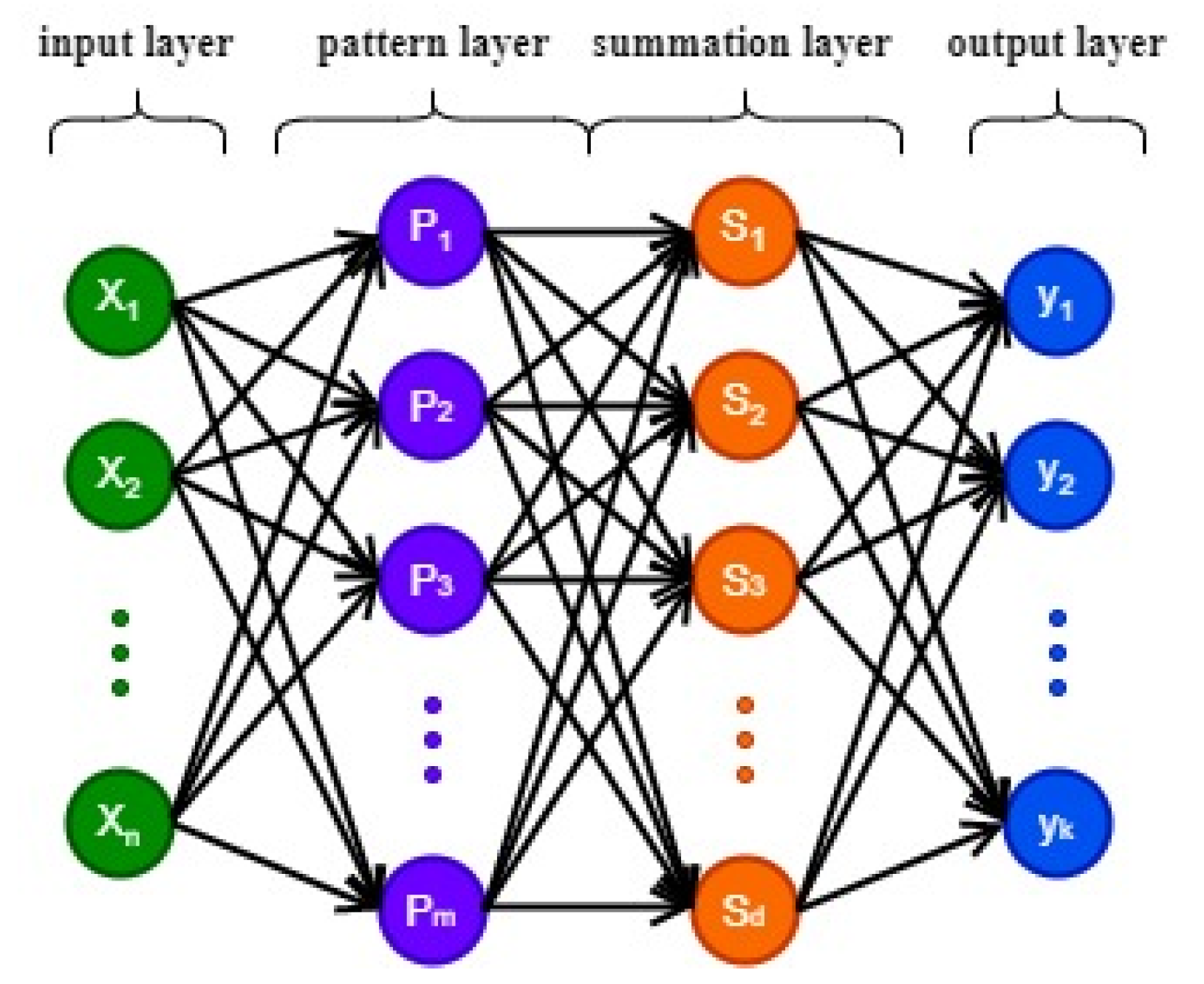
GRNN is a type of radial basis network that employs non-parametric regression and uses sample data as the posterior condition. It does not require backpropagation to find model parameters; therefore, GRNN is also a forward propagation network. The network performs non-parametric estimation and calculates the network output according to the principle of maximum probability. As shown in Figure 1, GRNN has a four-layer network structure [35,36] including input, pattern, summation, and output layers. In the figure, represents the output results, which can be obtained from by GRNN.
The input layer is used to input the parameters () of the learning sample, which are then passed to the pattern layer. The node’s number is equal to the number of input parameters.
The pattern layer receives input parameters from the input layer, and the number of nodes in the pattern layer is equal to the number of learning samples received. Each neuron node corresponds to an independent sample. The transfer function of neural node i is expressed by :
where X is the input variable, Xi is the learning sample corresponding to the i-th neuron, and is the standard deviation of the input parameter, which is also known as the smoothing factor.
Two types of summation methods are used for the summation layer, as shown by Equations (2) and (3). Although one output value is used, which is expressed by for type 1 in Equation (2), multiple output values are expressed by for type 2 in Equation (3), the number of which is the same as the number of output parameters:
where is the weight connecting the i-th neuron in the pattern layer to the summation layer [25,36,37], m is the number of neurons in the pattern layer, and is the number of output values.
The number of nodes in the output layer is the same as the number of output parameters, and the value of neural node k can be expressed by as
2.2. Case Study
Released by the United States Environmental Protection Agency (U.S. EPA), SWMM is an open-source public software program offered for free use worldwide. It is widely used in hydrological analysis with many successful applications. SWMM 5.1.015, released on 20 July 2020, was used for the simulation. This version can be downloaded from the agency’s website at https://www.epa.gov/water-research/storm-water-management-model-swmm (accessed on 28 January 2021).
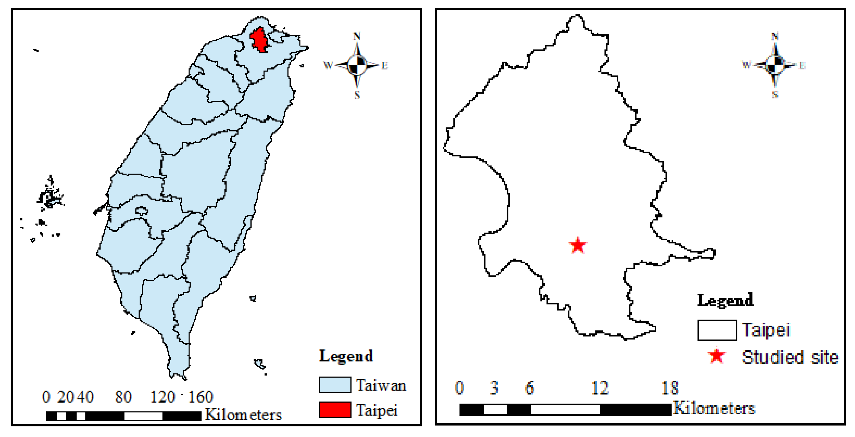
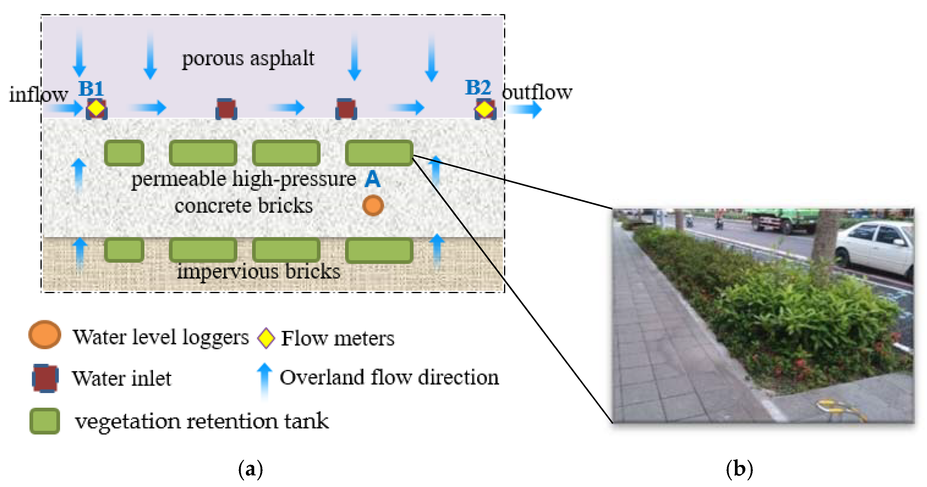
A large catchment can often be divided into multiple sub-catchments, such as that formed by permeable pavement found in great abundance in association with the sponge city proposal. The study area is Daan Road near the National Taipei University of Technology in Taiwan, as shown in Figure 2. Figure 3 presents a schematic diagram of the study area. As shown in Figure 3a, flowmeters were placed at the inflow and outflow points of the Daan research area to monitor the runoff changes in this area. To ensure the reliability of the observation values of the runoff flow rates, groundwater level loggers were set. The catchment area is 687.54 m2, and comprises porous asphalt, a vegetation retention tank, permeable high-pressure concrete bricks, and impervious bricks with areas of 181.04 m2, 100.6 m2, 245.7 m2, and 160.2 m2, respectively. It should be noted that, as shown in Figure 3b, the vegetation retention tank is designed to be an independent sub-catchment. Therefore, the catchment in the study area was divided into two sub-catchments. Sub-catchment 1 includes the permeable pavement and impervious bricks, and sub-catchment 2 contains only the vegetation retention tank. The porous asphalt and permeable high-pressure concrete bricks contained in sub-catchment 1 are considered to be permeable pavement; thus, the permeable pavement area is 426.74 m2.
Sensitivity analysis is a regular step in hydrological analysis and is used to assess the relationship between the input parameters and the output targets. Changing the value of an input parameter and ensuring that the other parameters remain unchanged is the most widely used method in such analysis. Many parameters are used to represent the sub-catchment characteristics in SWMM; nine of these parameters are most frequently reported in previous sensitivity analysis studies using this method [38]. The basic values for the catchment in this study are given in Table 1. For sub-catchment 1, several parameter values were easily obtained, while others were not. For example, the Destore–Perv parameter was difficult to obtain; however, its value in previous research is considered to be very small. Here, its value was set to 5 mm. During SWMM analysis, Horton was set as the infiltration model because its parameters are easily obtained by performing the penetration test onsite. For N-Imprev and N-perv, the recommended value in the SWMM manual, which is 0.012, was taken. The width (W) and slope (S) of sub-catchment 1 were not easily determined because a definitive overland flow path could not be identified. However, these parameters are important for predicting the runoff volume. According to the Manning formula, the runoff is closely related to S and W in Equations (5) and (6), respectively. Therefore, these parameters were selected as the variable parameters in SWMM:
where is the flow rate, is the runoff velocity, is the Manning factor, is the hydraulic radius, is the slope of sub-catchment, is the cross-section area, is the characteristic width of the overland flow path, and is the runoff depth.
In the sensitivity analysis of rainfall and runoff, the peak flow () and total flow volume () of runoff are computed as the output target. In addition to these parameters, the time to peak () is also an important target. However, in this case, because the monitoring data are updated every 10 min, is not easily confirmed and was thus ignored in this study. Onsite monitoring revealed that runoff data can be obtained even in the absence of rainfall; thus, a particular amount of external water affects the monitoring results in such cases. Therefore, to lower the impact of water from an unknown source on the runoff as much as possible, is calculated by the total flow volume during rainfall events only.
In summary, because the values of and can be obtained by observation, they were selected as representative characteristics in the hydrological simulation. The W and S of sub-catchment 1 were chosen to be predicted by GRNN under rainfall events. The rainfall data were collected from a rain gauge installed near the venue.
2.3. Method
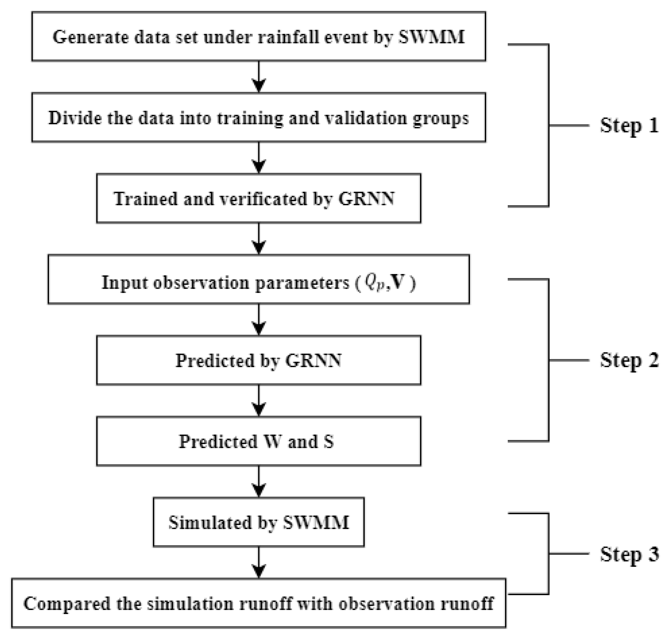
The research steps are shown in Figure 4. In Step 1, a training data set generated by SWMM was built for GRNN. As shown in Table 1, for sub-catchment 1, W and S are variables, and the values of the remaining parameters are constants. The basic value of W (S) in this case was 5 m (0.2%) and varied from 1 m to 10 m (0.1% to 0.3%). Ten values of W and eleven values of S were evenly distributed among their ranges for the SWMM simulation. The results of the runoff parameters (,) were recorded when SWMM simulated the hydrological response of the study area under a specific rainfall event.
In Step 2, the training data were divided randomly into two parts for training and verification, respectively. For training the data used in GRNN, the input parameters were , and the output parameters were . Because the amount of training data is limited, a cross-validation method was adopted to train the GRNN, and a loop was used to find the best smoothing factor. In this way, GRNN does not require abundant training data to obtain better training results. After the training was completed by GRNN, inputs and were obtained from the observed runoff curve to predict W and S by GRNN.
In Step 3, after the values of W and S were obtained from GRNN, they were input into SWMM for simulation to obtain the runoff parameters (,). Then, the simulation and observed runoff curves were compared.
2.4. Performance Criteria
- 1.
- Root-Mean-Square ErrorRoot-mean-square error (RMSE) is used to measure the deviation between the observed value and the true value and is defined aswhere is the input parameter, is the output or simulated parameter, and is the total number of input parameters. The RMSE range is between 0 and +∞.
- 2.
- Mean Absolute Percentage ErrorThe mean absolute percentage error (MAPE) is used to measure the relative error between the average test value and the real value of the test set and is defined aswhere the MAPE is between 0 and +∞. A calculated value close to zero reflects good fit in the prediction. However, it is worth noting that the formula cannot be used when the actual value is equal to zero because the denominator cannot be divided by zero.
- 3.
- Nash–Sutcliffe Efficiency CoefficientThe Nash–Sutcliffe efficiency coefficient (NSE) is defined aswhere is the average value of input parameters. The NSE range is between 1 and −∞, with calculated values close to 1 reflecting better fit for the prediction.
3. Results and Discussion
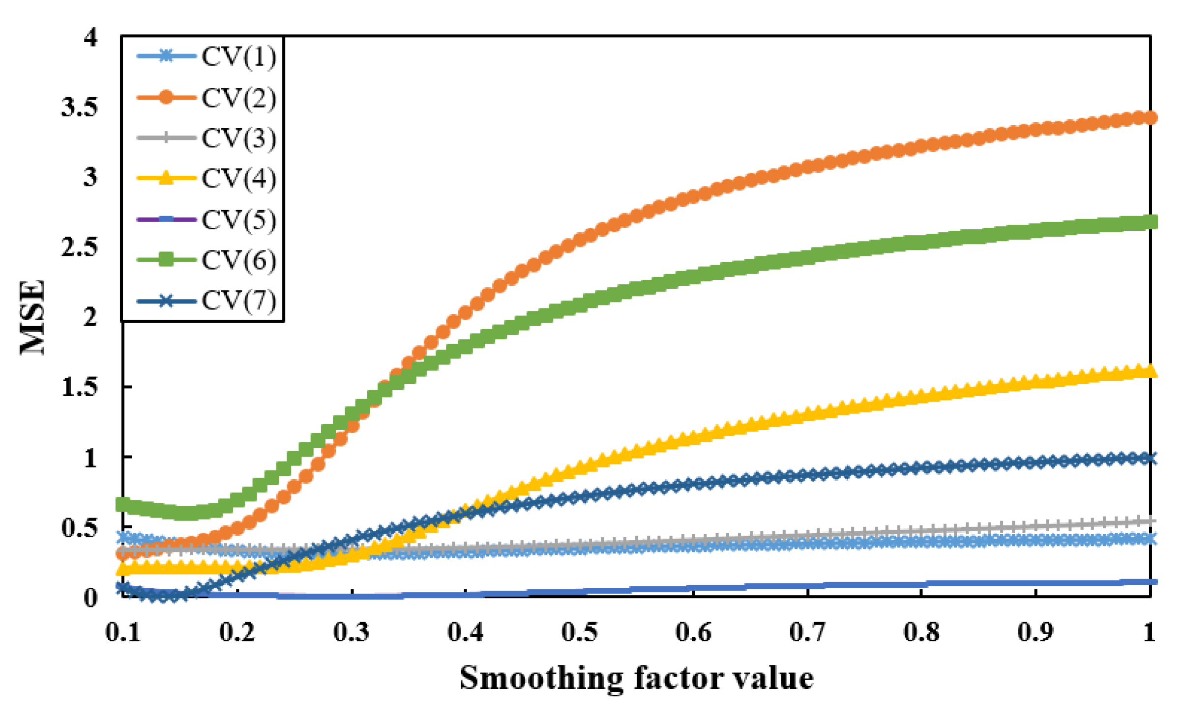
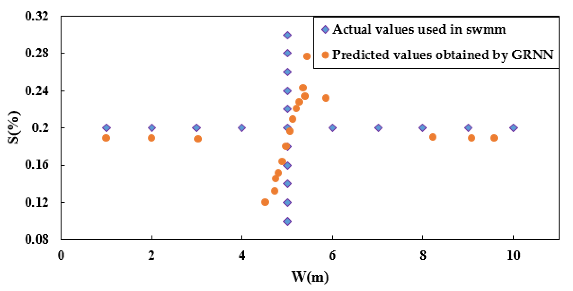
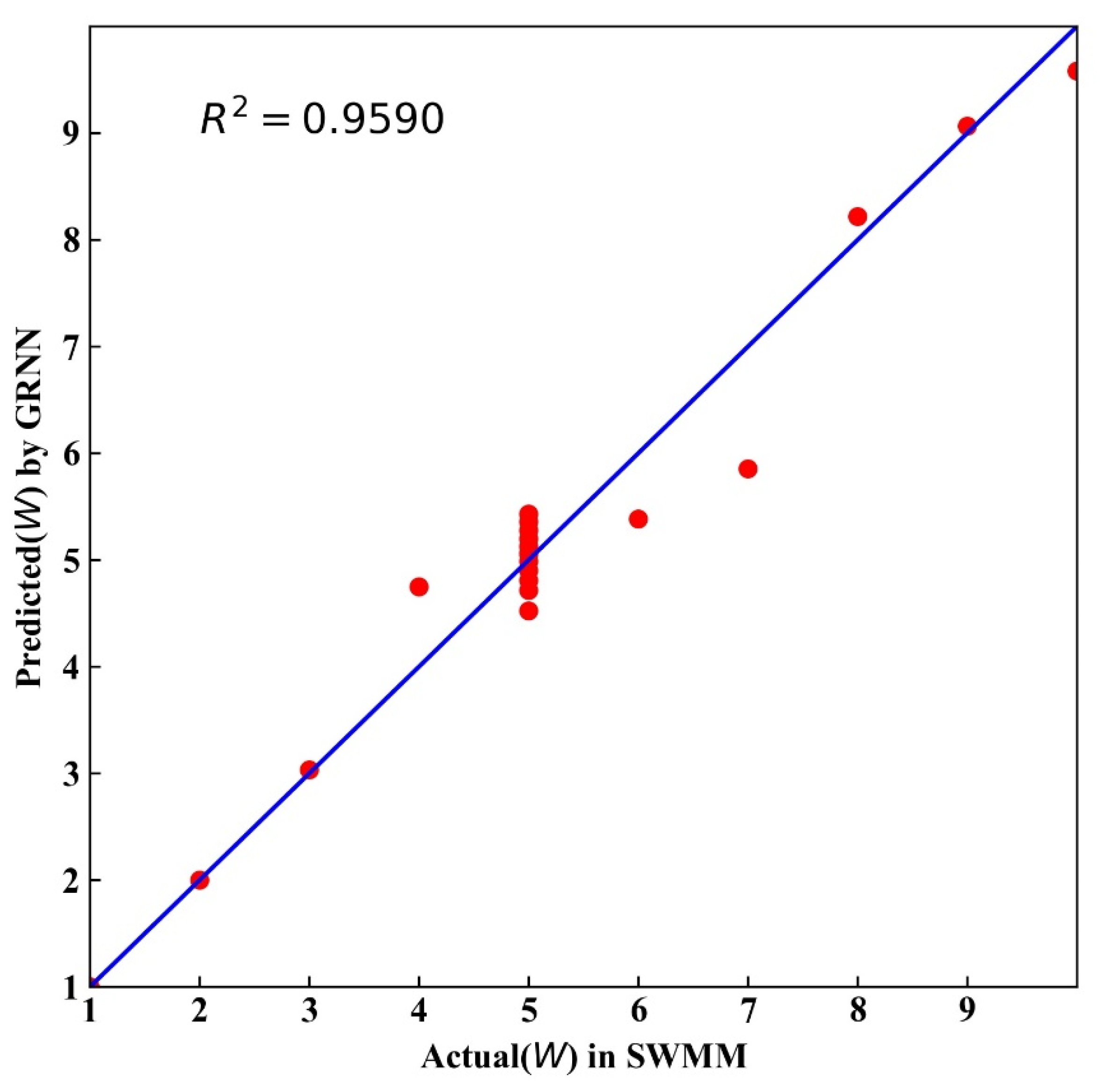
During the training phase, the values of W and S predicted by GRNN were compared with their actual values used in SWMM. The GRNN was implemented in Matlab. Because the performance of GRNN depends strongly on the value of the smoothing factor, the determination of this factor is of great importance. Therefore, the training data sets were experimentally simulated with different smoothing factors. The estimated results of the statistical error analysis are shown in Figure 5. A smoothing factor constant of 0.13 predicted satisfactory results because of it had the lowest MSE. Alternatively, the predicted values can have a smaller error than the actual values. The hyperparameters for GRNN are illustrated in Table 2. As shown in Figure 6, for each W and S couple, most of the predicted values were close to the actual values, which demonstrates that, with the exception of a few points, the GRNN performance was satisfactory in this study. However, as shown in Figure 7, the actual S equaled 0.2; therefore, the predicted values deviated greatly from the actual values. This phenomenon also appears in Figure 8 when the actual W equaled 5. This occurred because the basic values of W and S had more training data in GRNN relative to other values. To further verify whether this method is feasible, Table 3 shows the performance of the predicted parameters. These values indicate acceptable performance; therefore, the method of using GRNN to train the data set and then predicting the values of the parameters needed in SWMM has good accuracy.
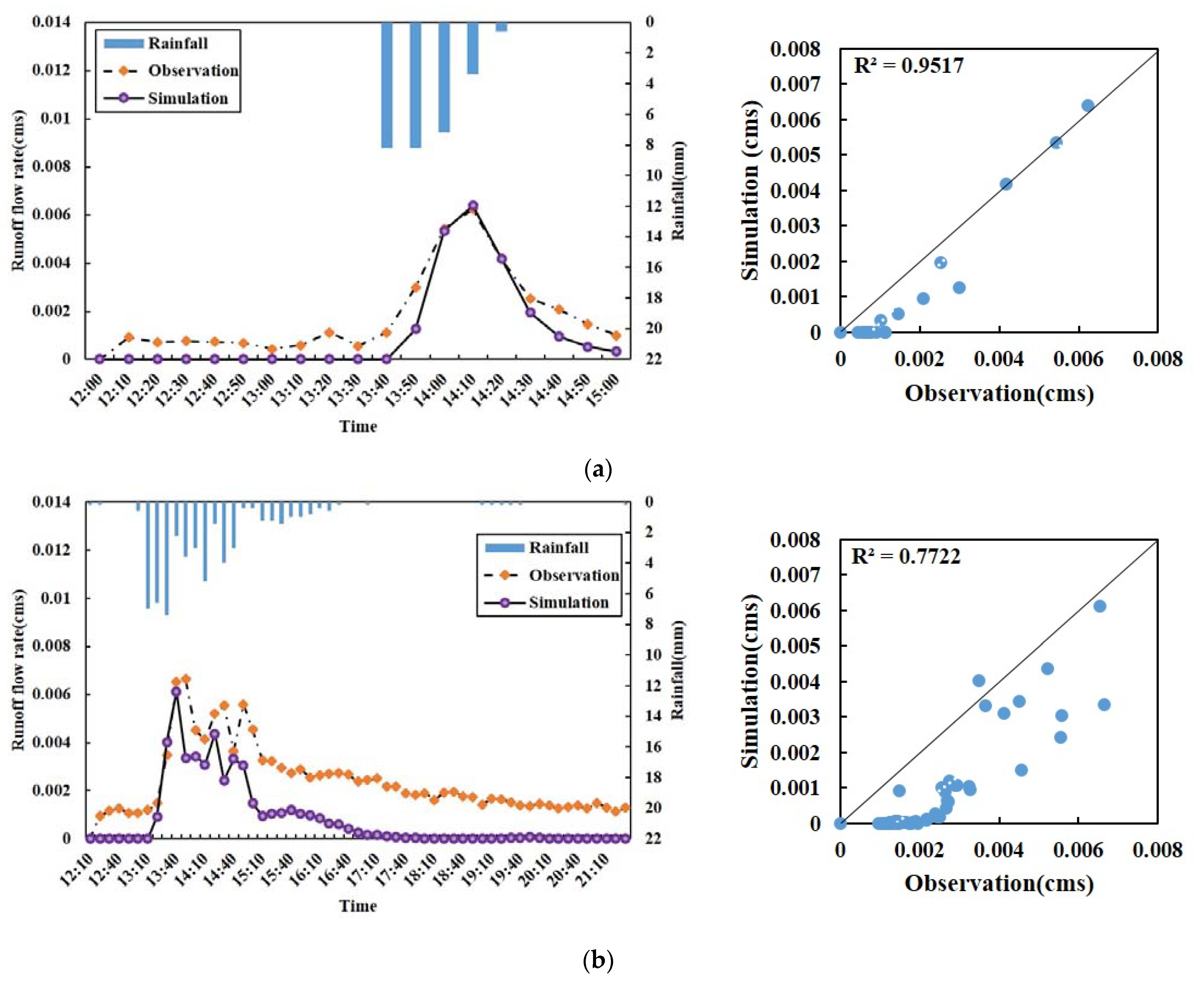
Although the predicted values of W and S appear to be satisfactory, the predicted values were still not perfectly equal to the actual values. For engineering practices, however, the actual effect is more important than the true value of the internal parameters. Therefore, the runoff curve was simulated in both the calibration (events of 24 July 2018) and validation (events of 30 August 2018) steps using the predicted W and S.
Figure 9 shows the relationship between the simulated and observed runoff curves. When rainfall occurred at 13:40 local time, the observed values were very close to the simulated values, particularly for , where the simulated value was approximately equal to the observed value. Although the predicted W and S were effective in the peak flow simulation by SWMM, the total flow volume () was underestimated. In addition, runoff data onsite were recorded before the rainfall occurred (Figure 8) because the monitoring data onsite were affected by external water from unknown sources. The study area is a public space; thus, it is difficult to obtain undisturbed monitoring data. The values were 0.9517 and 0.7722 for the calibration and validation, respectively, which indicate acceptable performance. In summary, the GRNN method can effectively predict the parameters needed in SWMM simulation. By using this method, reasonable parameters can easily be found for simulating runoff, which will be helpful for parameter calibration and verification using SWMM.
4. Conclusions
A method is proposed to study the potentiality of realizing the inversion of hydrological parameters for SWMM simulation. To reflect the feasibility of the predicted parameters in GRNN, three indicators were used to evaluate the performance of the model. For input parameters (, ), predicted parameters (W, S) were determined by GRNN. and were then used to simulate the runoff flow rates by SWMM. A comparison of the simulated runoff curve and observed runoff curves revealed that the proposed method is suitable for predicting the hydrological parameters with acceptable accuracy.
Nevertheless, many situations in different study areas require the prediction of more than two parameters. The present research represents one case study, but many difficulties remain for applying neural network-like methods to other engineering cases. This aspect of using an ANN method for integrating research software, such as that combined with SWMM, is to be considered in future research.
Author Contributions
Conceptualization, Q.-C.C., T.-H.H. and J.-Y.L.; methodology, Q.-C.C.; software, Q.-C.C.; validation, Q.-C.C., T.-H.H. and J.-Y.L.; formal analysis, Q.-C.C.; investigation, J.-Y.L.; data curation, J.-Y.L.; writing—original draft preparation, Q.-C.C.; writing—review and editing, T.-H.H.; project administration, J.-Y.L. All authors have read and agreed to the published version of the manuscript.
Funding
This research received no external funding.
Institutional Review Board Statement
Not applicable.
Informed Consent Statement
Not applicable.
Data Availability Statement
The study did not report any data. We choose to exclude this statement.
Acknowledgments
The authors thank the reviewers and editor for their valuable comments, which helped improve the quality of this manuscript.
Conflicts of Interest
The authors declare no conflict of interest.
References
- Zhan, W.; Chui, T.F.M. Evaluating the life cycle net benefit of low impact development in a city. Urban For. Urban Green. 2016, 20, 295–304. [Google Scholar] [CrossRef]
- Baek, S.; Ligaray, M.; Pachepsky, Y.; Chun, J.A.; Yoon, K.-S.; Park, Y.; Cho, K.H. Assessment of a green roof practice using the coupled SWMM and HYDRUS models. J. Environ. Manag. 2020, 261, 109920. [Google Scholar] [CrossRef]
- Jiang, C.; Li, J.; Li, H.; Li, Y.; Zhang, Z. Low-impact development facilities for stormwater runoff treatment: Field monitoring and assessment in Xi’an area, China. J. Hydrol. 2020, 585, 124803. [Google Scholar] [CrossRef]
- Jia, H.; Lu, Y.; Yu, S.L.; Chen, Y. Planning of LID–BMPs for urban runoff control: The case of Beijing Olympic Village. Sep. Purif. Technol. 2012, 84, 112–119. [Google Scholar] [CrossRef]
- Degtyareva, O.; Degtyarev, G.; Togo, I.; Terleev, V.; Nikonorov, A.; Volkov, Y. Analysis of Stress-strain State Rainfall Runoff Control System–Buttress Dam. Procedia Eng. 2016, 165, 1619–1628. [Google Scholar] [CrossRef]
- Tedoldi, D.; Chebbo, G.; Pierlot, D.; Kovacs, Y.; Gromaire, M.-C. Impact of runoff infiltration on contaminant accumulation and transport in the soil/filter media of Sustainable Urban Drainage Systems: A literature review. Sci. Total. Environ. 2016, 569-570, 904–926. [Google Scholar] [CrossRef] [PubMed]
- Zhang, P.; Cai, Y.; Wang, J. A simulation-based real-time control system for reducing urban runoff pollution through a stormwater storage tank. J. Clean. Prod. 2018, 183, 641–652. [Google Scholar] [CrossRef]
- Ahmadi, M.; Moeini, A.; Ahmadi, H.; Motamedvaziri, B.; Zehtabiyan, G.R. Comparison of the performance of SWAT, IHACRES and artificial neural networks models in rainfall-runoff simulation (case study: Kan watershed, Iran). Phys. Chem. Earth Parts A/B/C 2019, 111, 65–77. [Google Scholar] [CrossRef]
- Srivastava, A.; Kumari, N.; Maza, M. Hydrological Response to Agricultural Land Use Heterogeneity Using Variable Infiltration Capacity Model. Water Resour. Manag. 2020, 34, 3779–3794. [Google Scholar] [CrossRef]
- Srivastava, A.; Sahoo, B.; Raghuwanshi, N.S.; Singh, R. Evaluation of Variable-Infiltration Capacity Model and MODIS-Terra Satellite-Derived Grid-Scale Evapotranspiration Estimates in a River Basin with Tropical Monsoon-Type Climatology. J. Irrig. Drain. Eng. 2017, 143, 04017028. [Google Scholar] [CrossRef] [Green Version]
- Tsihrintzis, V.A.; Hamid, R. Runoff quality prediction from small urban catchments using SWMM. Hydrol. Process. 1998, 12, 311–329. [Google Scholar] [CrossRef]
- Costabile, P.; Costanzo, C.; Ferraro, D.; Macchione, F.; Petaccia, G. Performances of the New HEC-RAS Version 5 for 2-D Hydrodynamic-Based Rainfall-Runoff Simulations at Basin Scale: Comparison with a State-of-the Art Model. Water 2020, 12, 2326. [Google Scholar] [CrossRef]
- Hossain, S.; Hewa, G.A.; Wella-Hewage, S. A Comparison of Continuous and Event-Based Rainfall–Runoff (RR) Modelling Using EPA-SWMM. Water 2019, 11, 611. [Google Scholar] [CrossRef] [Green Version]
- Paul, P.K.; Kumari, N.; Panigrahi, N.; Mishra, A.; Singh, R. Implementation of cell-to-cell routing scheme in a large scale conceptual hydrological model. Environ. Model. Softw. 2018, 101, 23–33. [Google Scholar] [CrossRef]
- Niazi, M.; Nietch, C.; Maghrebi, M.; Jackson, N.; Bennett, B.R.; Tryby, M.; Massoudieh, A. Storm Water Management Model: Performance Review and Gap Analysis. J. Sustain. Water Built Environ. 2017, 3, 04017002. [Google Scholar] [CrossRef] [PubMed] [Green Version]
- Cheng, Y.-Y.; Lo, S.-L.; Ho, C.-C.; Lin, J.-Y.; Yu, S.L. Field Testing of Porous Pavement Performance on Runoff and Temperature Control in Taipei City. Water 2019, 11, 2635. [Google Scholar] [CrossRef] [Green Version]
- Tsai, L.-Y.; Chen, C.-F.; Fan, C.-H.; Lin, J.-Y. Using the HSPF and SWMM Models in a High Pervious Watershed and Estimating Their Parameter Sensitivity. Water 2017, 9, 780. [Google Scholar] [CrossRef] [Green Version]
- Chang, T.-Y.; Chen, H.; Fu, H.-S.; Chen, W.-B.; Yu, Y.-C.; Su, W.-R.; Lin, L.-Y. An Operational High-Performance Forecasting System for City-Scale Pluvial Flash Floods in the Southwestern Plain Areas of Taiwan. Water 2021, 13, 405. [Google Scholar] [CrossRef]
- Chang, H.-K.; Lin, Y.-J.; Lai, J.-S. Methodology to set trigger levels in an urban drainage flood warning system–An application to Jhonghe, Taiwan. Hydrol. Sci. J. 2017, 63, 31–49. [Google Scholar] [CrossRef]
- Del Giudice, G.; Padulano, R. Sensitivity Analysis and Calibration of a Rainfall-Runoff Model with the Combined Use of EPA-SWMM and Genetic Algorithm. Acta Geophys. 2016, 64, 1755–1778. [Google Scholar] [CrossRef] [Green Version]
- Hamouz, V.; Muthanna, T.M. Hydrological modelling of green and grey roofs in cold climate with the SWMM model. J. Environ. Manag. 2019, 249, 109350. [Google Scholar] [CrossRef] [PubMed]
- Gao, X.; Yang, Z.; Han, D.; Huang, G.; Zhu, Q. A Framework for Automatic Calibration of SWMM Considering Input Uncertainty. Hydrol. Earth Syst. Sci. Discuss. 2020, 1–25. [Google Scholar] [CrossRef]
- Beven, K.; Freer, J. Equifinality, data assimilation, and uncertainty estimation in mechanistic modelling of complex environ-mental systems using the GLUE methodology. J. Hydrol. 2001, 249, 11–29. [Google Scholar] [CrossRef]
- Biondi, D.; De Luca, D. Performance assessment of a Bayesian Forecasting System (BFS) for real-time flood forecasting. J. Hydrol. 2013, 479, 51–63. [Google Scholar] [CrossRef]
- Krzysztofowicz, R. Bayesian system for probabilistic river stage forecasting. J. Hydrol. 2002, 268, 16–40. [Google Scholar] [CrossRef]
- Srinivasulu, S.; Jain, A. A comparative analysis of training methods for artificial neural network rainfall–runoff models. Appl. Soft Comput. 2006, 6, 295–306. [Google Scholar] [CrossRef]
- Kumar, A.R.S.; Sudheer, K.P.; Jain, S.K.; Agarwal, P.K. Rainfall-runoff modelling using artificial neural networks: Comparison of network types. Hydrol. Process. 2005, 19, 1277–1291. [Google Scholar] [CrossRef]
- Asadi, H.; Shahedi, K.; Jarihani, B.; Sidle, R.C. Rainfall-Runoff Modelling Using Hydrological Connectivity Index and Artificial Neural Network Approach. Water 2019, 11, 212. [Google Scholar] [CrossRef] [Green Version]
- Yadav, A.K.; Chandola, V.K.; Singh, A.; Singh, B.P. Rainfall-Runoff Modelling Using Artificial Neural Networks (ANNs) Model. Int. J. Curr. Microbiol. Appl. Sci. 2020, 9, 127–135. [Google Scholar] [CrossRef]
- Kumari, N.; Acharya, S.C.; Renzullo, L.J.; Yetemen, O. Applying rainfall ensembles to explore hydrological uncertainty. In Proceedings of the 23rd International Congress on Modelling and Simulation, Canberra, Australia, 1–6 December 2019; pp. 1070–1076. [Google Scholar] [CrossRef]
- Apaydin, H.; Feizi, H.; Sattari, M.T.; Colak, M.S.; Shamshirband, S.; Chau, K.-W. Comparative Analysis of Recurrent Neural Network Architectures for Reservoir Inflow Forecasting. Water 2020, 12, 1500. [Google Scholar] [CrossRef]
- Erkan, M.; Turan, M. Ali Yurdusev, River flow estimation from upstream flow records by artificial intelligence methods. J. Hydrol. 2009, 369, 71–77. [Google Scholar] [CrossRef]
- Lee, J.; Lee, J.E.; Kim, N.W. Estimation of Hourly Flood Hydrograph from Daily Flows Using Artificial Neural Network and Flow Disaggregation Technique. Water 2020, 13, 30. [Google Scholar] [CrossRef]
- Wan, H.; Bian, J.; Wu, J.; Sun, X.; Wang, Y.; Jia, Z. Prediction of Seasonal Frost Heave Behavior in Unsaturated Soil in Northeastern China Using Interactive Factor Analysis with Split-Plot Experiments and GRNN. Water 2019, 11, 1587. [Google Scholar] [CrossRef] [Green Version]
- Ghritlahre, H.K.; Prasad, R.K. Exergetic performance prediction of solar air heater using MLP, GRNN and RBF models of artificial neural network technique. J. Environ. Manag. 2018, 223, 566–575. [Google Scholar] [CrossRef] [PubMed]
- Izonin, I.; Tkachenko, R.; Verhun, V.; Zub, K. An approach towards missing data management using improved GRNN-SGTM en-semble method. Eng. Sci. Technol. Int. J. 2020. [Google Scholar] [CrossRef]
- First, M.; Turan, M.E.; Yurdusev, M.A. M.; Turan, M.E.; Yurdusev, M.A. Comparative analysis of neural network techniques for predicting water consumption time series. J. Hydrol. 2010, 384, 46–51. [Google Scholar] [CrossRef]
- Behrouz, M.S.; Zhu, Z.; Matott, L.S.; Rabideau, A.J. A new tool for automatic calibration of the Storm Water Management Model (SWMM). J. Hydrol. 2020, 581, 124436. [Google Scholar] [CrossRef]
- Talei, A.; Chua, L.H.C.; Quek, C.; Jansson, P.-E. Runoff forecasting using a Takagi–Sugeno neuro-fuzzy model with online learning. J. Hydrol. 2013, 488, 17–32. [Google Scholar] [CrossRef]
- Alizadeh, M.J.; Kavianpour, M.R.; Kisi, O.; Nourani, V. A new approach for simulating and forecasting the rainfall-runoff process within the next two months. J. Hydrol. 2017, 548, 588–597. [Google Scholar] [CrossRef]
- He, X.; Luo, J.; Zuo, G.; Xie, J. Daily Runoff Forecasting Using a Hybrid Model Based on Variational Mode Decomposition and Deep Neural Networks. Water Resour. Manag. 2019, 33, 1571–1590. [Google Scholar] [CrossRef]
Figure 1.
Schematic diagram of the architecture of the general regression neural network (GRNN).

Figure 2.
Location of the study site in Taipei city. The left-hand image shows the location of the city, and that on the right shows the study area.
Figure 2.
Location of the study site in Taipei city. The left-hand image shows the location of the city, and that on the right shows the study area.

Figure 3.
Schematic diagram of the study area: (a) onsite monitoring locations; (b) photograph of the vegetation retention tank onsite.
Figure 3.
Schematic diagram of the study area: (a) onsite monitoring locations; (b) photograph of the vegetation retention tank onsite.

Figure 4.
Schematic diagram of the three proposed research steps. Note: SWMM—storm water management model; GRNN—general regression neural network; Qp—peak flow; V—total flow volume; W—width; S—slope.
Figure 4.
Schematic diagram of the three proposed research steps. Note: SWMM—storm water management model; GRNN—general regression neural network; Qp—peak flow; V—total flow volume; W—width; S—slope.

Figure 5.
Effect of smoothing factor on GRNN performance under different cross-validations (CV(1)–CV(7)).
Figure 5.
Effect of smoothing factor on GRNN performance under different cross-validations (CV(1)–CV(7)).

Figure 6.
Relationship between actual values used in storm water management model (SWMM) and predicted values obtained by GRNN.
Figure 6.
Relationship between actual values used in storm water management model (SWMM) and predicted values obtained by GRNN.

Figure 7.
Relationship between actual width (W) and predicted W values.

Figure 8.
Relationship between actual slope (S) and predicted S values.

Figure 9.
Comparison of observed and simulated runoff values using model-calibrated parameters: (a) calibration; (b) validation.
Figure 9.
Comparison of observed and simulated runoff values using model-calibrated parameters: (a) calibration; (b) validation.


Table 1.
Storm water management model (SWMM) parameters used in the case study.
| Parameters | Sub-Catchment 1 | Sub-Catchment 2 |
|---|---|---|
| Area (ha) | 0.058694 | 0.01006 |
| Width (m) | 1–10, Basic value: 5 | 8 |
| Slope (%) | 0.1–0.3, Basic value: 0.2 | 0.1 |
| Imprev (%) | 27.23 | 0 |
| N-Imprev | 0.012 | — |
| N-perv | 0.012 | 0.04 |
| Destore Imprev (mm) | 5 | — |
| Destore–Perv (mm) | 5 | 0.2 |
| Infil. Model | Horton | Horton |
| Zero Imperv (%) | — | — |
Table 2.
The hyperparameters for best results with GRNN.
| Hyperparameter | Value |
|---|---|
| The number of neurons in input layer | 2 |
| The number of neurons in pattern layer | 18 |
| The number of neurons in summation layer | 2 |
| The number of neurons in output layer | 2 |
| Smoothing factor | 0.13 |
Table 3.
Comparison of simulation results for evaluating the method performance.
| Parameter | RMSE | MAPE | NSE |
|---|---|---|---|
| W | 0.3946 | 5.04% | 0.9950 |
| S | 0.0219 | 8.78% | 0.9878 |
Note: RMSE—root-mean-square error; MAPE—mean absolute percentage error; NSE— Nash–Sutcliffe efficiency coefficient.
Publisher’s Note: MDPI stays neutral with regard to jurisdictional claims in published maps and institutional affiliations. |
© 2021 by the authors. Licensee MDPI, Basel, Switzerland. This article is an open access article distributed under the terms and conditions of the Creative Commons Attribution (CC BY) license (https://creativecommons.org/licenses/by/4.0/).
Share and Cite
MDPI and ACS Style
Cai, Q.-C.; Hsu, T.-H.; Lin, J.-Y. Using the General Regression Neural Network Method to Calibrate the Parameters of a Sub-Catchment. Water 2021, 13, 1089. https://doi.org/10.3390/w13081089
AMA Style
Cai Q-C, Hsu T-H, Lin J-Y. Using the General Regression Neural Network Method to Calibrate the Parameters of a Sub-Catchment. Water. 2021; 13(8):1089. https://doi.org/10.3390/w13081089
Chicago/Turabian StyleCai, Qing-Chi, Tsung-Hung Hsu, and Jen-Yang Lin. 2021. "Using the General Regression Neural Network Method to Calibrate the Parameters of a Sub-Catchment" Water 13, no. 8: 1089. https://doi.org/10.3390/w13081089
Note that from the first issue of 2016, this journal uses article numbers instead of page numbers. See further details here.