
Determination of Optimal Meshness of Sewer Network Based on a Cost—Benefit Analysis


Department of Hydrosciences, Institute for Urban Water Management, TU Dresden, 01069 Dresden, Germany
*
Author to whom correspondence should be addressed.
Water 2021, 13(8), 1090; https://doi.org/10.3390/w13081090
Submission received: 23 March 2021
/
Revised: 13 April 2021
/
Accepted: 13 April 2021
/
Published: 15 April 2021
(This article belongs to the Section Urban Water Management)
Abstract
:Urban pluvial flooding occurs when the capacity of sewer networks is surcharged due to large amounts runoff produced during intense rain events. Rapid urbanization processes and changes in climate increase these events frequency. Effective and sustainable approaches for the reduction in urban floods are necessary. Although several gray, green and hybrid measures have been studied, the influence of network structure on flood occurrence has not yet been systematically evaluated. This study focuses on evaluating how different structures of a single urban drainage network affect flood volumes and their associated damages. Furthermore, a cost–benefit analysis is used to determine the best network structure. As a case study, a sewer subnetwork in Dresden, Germany was selected. Scenarios corresponding to different layouts are developed and evaluated using event-wise hydrodynamic simulation. The results indicate that more meshed structures are associated with lower flood volumes and damage. Moreover, all analyzed scenarios were identified as cost-effective, i.e., the benefits in terms of flood damage reduction outweighed the costs related to pipe installation, operation and maintenance. However, a predominantly branched structure was identified as the best scenario. The present approach may provide a new cost-effective solution that can be integrated into the development of different mitigation strategies for flood management.
1. Introduction
In recent decades, increases in population and urbanization processes have led to an expansion of impervious areas. These processes cause a disturbance in the natural hydrological processes, leading to an increased generation of runoff volumes and higher runoff peaks [1,2]. In urban areas, this excess water is typically collected by sewer networks and transported into specific outlet points such as wastewater treatment plants or nearby water bodies. Nevertheless, these systems have a limited capacity. Depending on the physical characteristics of the contributing area (e.g., population density, land use types or topography), the system’s design capacity can vary [3,4]. Sewer systems are design based on a predefined “satisfactory service level”, which represents the degree of protection against flooding, and it is mainly associated with a selected synthetic design storm event [4]. The recurrence interval of these design storms can vary from one to ten years, depending on the type and properties of the drainage area [3].
Rain events with a higher intensity and/or duration than the design storms may lead to a surcharge of the sewer network’s capacity. In combined sewers, the excess water, typically a mixture of sewage, extraneous water and stormwater, is released from the system through overflowing manholes and gully pots into the surface. This type of flood, referred to typically as urban pluvial flood, has been identified as one of the main hazards to modern towns and cities due to its potential societal and environmental impacts, and economical and structural damage [5,6,7,8,9].
The development of effective and sustainable approaches for the reduction in urban pluvial floods thus has become relevant. Such approaches aim for the reduction or better management of the large runoff quantities generated during intense rain events. Intervention strategies are typically classified either as green solutions, i.e., decentralized measures to manage runoff at the source, or grey solutions, focused on the improvement of the network’s capacity. In this latter case, the available storage is typically increased by constructing stormwater tanks or increasing the dimensions of the existing infrastructure, for example by installing pipes with bigger diameters
Although these are efficient solutions for reducing pluvial flood risks, recent studies have also suggested that the physical arrangement, i.e., the layout, of the sewer network may play an important role in the occurrence and magnitude of pluvial flood events. Zhang et al. [10] suggested that sewer networks with a more meshed structure are less vulnerable to structural failures, e.g., blockages, and are associated with lower flooding volumes than systems with a tree-like structure. Reyes-Silva et al. [11] analyzed the influence of network structure, quantified in terms of a Meshness coefficient, on the occurrence and magnitude of node flooding using eight different sewer networks. The obtained results suggest that networks with higher Meshness values, i.e., structures with a more mesh-like layout, are more reliable in terms of flooded nodes and flooding volumes than systems with a predominantly branched structure. Nevertheless, the effects of varying the Meshness in a single network and its implication for node flooding remain unclear. Hesarkazzazi et al. [12] studied the effect of redundancy in stormwater drainage systems, represented as the presence of loops in the network structure. The outcomes of this study suggest that systems with a more looped structure are associated with lower flooding volumes but higher investment costs due to the installation of additional pipes that provided the loops, i.e., redundancy in the system.
In this context, this study focuses on two main research goals. First, the effects of varying the network structure (i.e., layout) on the magnitude of pluvial flood events for a single urban drainage network (UDN) are analyzed. The different structures are classified using the Meshness coefficient proposed by Reyes-Silva et al. [11]. In this approach, an UDN is represented as the graph (G = (E, V)), where the edges (E) correspond to pipe sections, while the vertices (V) are the junctions between them. The Meshness is then determined based on the number of pipes connected to those junctions which are not source or outlet nodes, referred as inner nodes. Meshness can vary between 0% and 100%, representing layouts with the least number of pipes without causing any disconnection, and with the maximum number of connected pipes per inner node, respectively. Furthermore, changes in UDN structure are obtained by adding or removing pipes. As a consequence, changes in layout are associated with different investment costs. Therefore, the second goal of this study is to determine the most appropriate layout which balances the incremental costs with the associated benefits of increasing Meshness. The analyzed benefits considered the reduction in flood damage as a consequence of reducing flood volumes. To perform these analyses, a sub-network from the sewer system of Dresden, Germany, located in the southeast region of the city, is selected as a case study. Flood occurrence and magnitude are obtained via hydrodynamic simulations.
2. Materials and Methods
2.1. Case Study
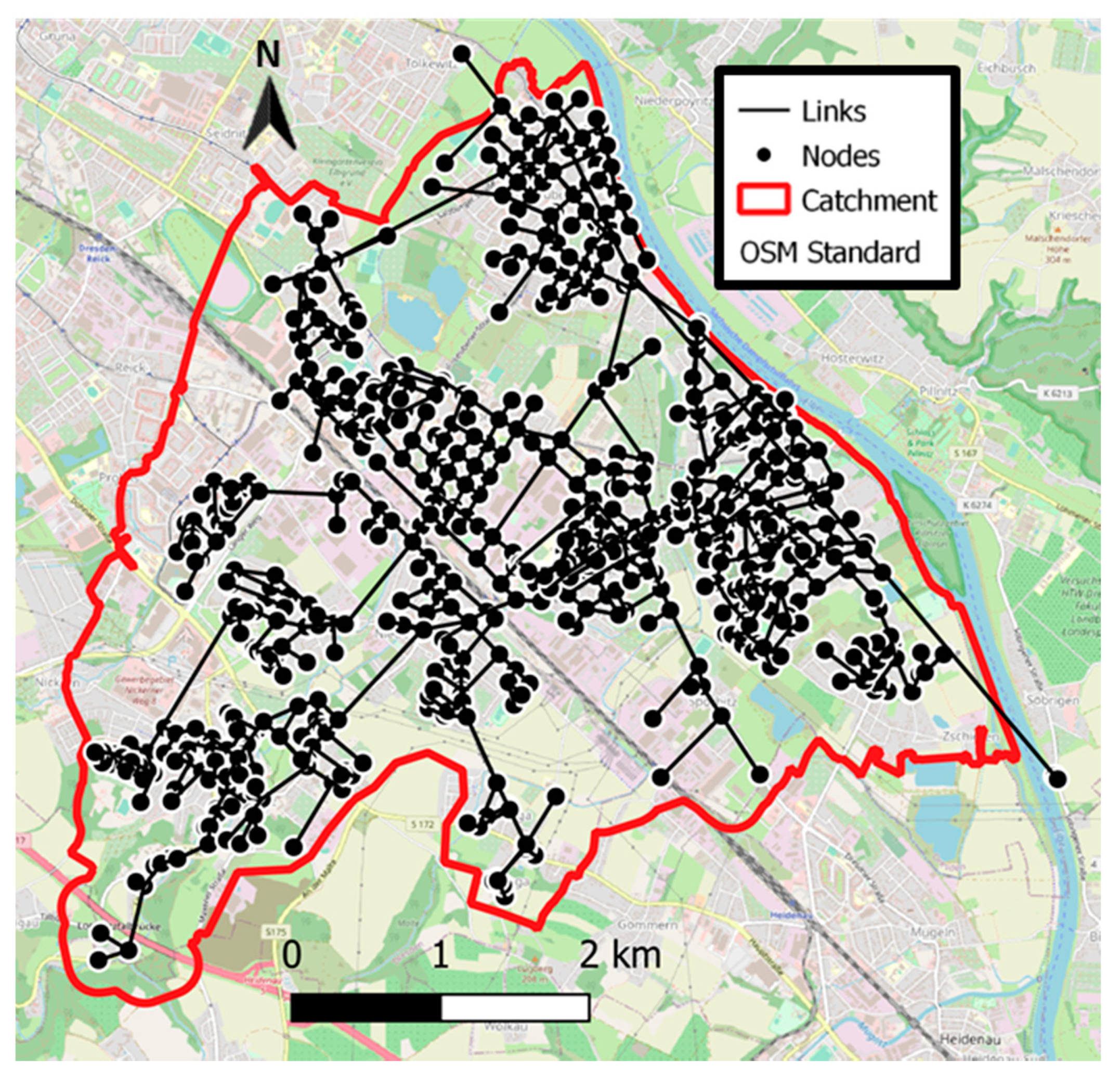
A sub-network from the sewer system of Dresden, Germany, located in the southeast region of the city, was selected as the study area (Figure 1). The total drainage area is approximately 24.3 km2, of which 42% corresponds to impervious surfaces. Furthermore, the local environmental, agricultural and geological agency has identified 28 different land uses in the area (see Figure A1 [13]). In order to simplify the flood damage analyses, these land uses are reclassified to match the categories used in the depth–damage curves proposed by Huizinga et al. [14]. These curves are used in this study for analyzing flood damage. Further information about this is provided in Section 2.5. and Appendix A. The study area is reclassified into six major land uses: Agriculture, Industry, Commerce, Residential, Infrastructure and No Damage. This last one corresponds to green areas where flooding is not expected to cause any economic damage. Information regarding the reclassification process can be found in Appendix A. The structure of the sewer systems is quantified using the Meshness coefficient proposed by Reyes-Silva et al. [11], which indicates whether the structure of a sewer network is predominantly branched or meshed. This coefficient ranges between 0% and 100%, representing a network structure with the minimum or maximum possible number connected pipes per node. The results show that the analyzed subnetwork has a predominantly branched structure, with a Meshness value of 25%.
2.2. Scenario Construction
Meshness is used as an indicator of an UDN structure. Therefore, the different scenarios developed in this study correspond to sewer network configurations, i.e., layouts with different Meshness degrees. As a starting point, the structures with the lowest and with the highest Meshness possible were determined. This was done in order to evaluate the maximum possible range in which the structure of the network can vary. On the one hand, the lowest Meshness scenario corresponds to the minimum spanning tree (MST) configuration, which represents the 0% Meshness conditions [11]. This network structure and its elements are identified using Kruskal’s algorithm [15]. On the other hand, although theoretically a network configuration of 100% Meshness can exist, it might not represent a realistic layout due to spatial restrictions. The highest Meshness that can be achieved is determined through an iterative procedure and based on a distance threshold (which accounts for spatial restrictions). For the current study area, a distance threshold of 400 m was used. As a result, the maximum Meshness possible for the analyzed UDN was 45%. For more information about this iterative process, see Reyes-Silva et al. [16].
After determining the maximum range of Meshness variability, scenarios with intermediate Meshness degrees, i.e., between 0% and 45%, were developed. The starting point for this was the original layout, which has a Meshness of 25%. On the one hand, configurations with Meshness degrees lower than the reference conditions (<25%) were determined by randomly removing the pipes which were not part of the MST from the original layout. This was done iteratively until Meshness values of 5%, 10%, 15% and 20% are obtained. Each of these corresponded then to a single scenario. On the other hand, network layouts with Meshness degrees higher than the reference condition were built by randomly adding pipe sections where topography and network connectivity allowed it. This was done by following a similar iterative procedure as the one used for determining the maximum Meshness possible. In this case, however, the process stopped every time the Meshness degree reached a value of 30%, 35% or 40%.
As a result, ten scenarios were developed and analyzed. These corresponded to UDN layouts with Meshness degrees between 0% and 45%, with a minimum Meshness difference of 5% among them. The main difference among the scenarios was the number of pipes present in the system. Other structural elements such as manholes, storage tanks and combined sewer overflows remained unchanged. Furthermore, contributing areas also remained constant among the different scenarios.
2.3. Hydrodynamic Simulations and Node Flooding
Hydrologic–hydraulic simulations were used to determine the location and magnitude of node flooding events in the study area and the different scenarios. For this, a previously developed hydrodynamic model of the study area, implemented in the EPA Stormwater Management Model (EPA SWMM) software [17], was used. For more information about this model and its development, see Reyes-Silva et al. [16]. Based on this model, the other nine scenarios are implemented. Scenarios with Meshness degrees lower than the reference condition (i.e., 25%) were obtained by simply deleting the pipes which were not part of these layouts, as identified in the scenario construction phase. Additionally, in the scenarios of 30% to 45% Meshness, conduits were added to the reference model incrementally to obtain the desired Meshness degree. The location of such links was determined previously during the scenario development phase. The hydraulic properties of these pipes (i.e., type of cross-section, maximum depth and roughness) were assumed to be similar to the ones from the upstream link. Furthermore, length was calculated based on the locations of the upstream and downstream nodes. Other pipe parameters in EPA SWMM, e.g., offsets or initial flow, were set to 0.
Event-based simulations were done to analyze the dynamics of node flooding in the different scenarios. For this study, four synthetic precipitation events were used. These corresponded to one-hour rain events with a return period of 10, 20, 50 and 100 years. They were ‘Euler Type II’ design storms [18], with reference precipitation intensities of the city of Dresden, Germany, according to the coordinated storm event intensities [19].
2.4. Flood Depth and Flooded Area Determination
The estimation of the flood depths and areas was done by coupling the EPA SWMM results with a surface diffusive overland flow model proposed by Chen et al. [20]. The total flooded volume from the surcharged junctions reported in the EPA SWMM results served as input in the diffusive overland flow model to simulate the surface flow and estimate surface inundation extension and depths. In this approach, the study area is arranged as a grid with uniform square cells. The surface elevation of each cell is defined by a 2 × 2 m2 digital surface model obtained from the state service for geoinformation and geodesy Saxony (Staatsbetrieb Geobasisinformation und Vermessung Sachsen (GeoSN)). Each individual cell acts as storage and the cells located above a flooding node are considered as source cells. These cells are initially filled with the corresponding flood volume reported in the EPA SWMM results. Then, if topography allows, the algorithm distributes the flooding water of each source cell to its eight adjacent dry cells. Flood water is allocated into a nearby cell only if the height of the source cell is higher than the nearby one, thus resembling gravitational surface flow. Based on the distributed volume and the number of cells with water, a flood depth is calculated. If this depth is higher than a given threshold, the new cells filled with water act as new source cells and the process continues iteratively until a depth threshold is reached. When the process is over, it is possible to analyze the extent of the flooded area and the flood depth associated with each flooded node in the study area. Although this approach neglects several hydrodynamic processes of surface water diffusion [20], its results are considered appropriate enough to analyze the effects of different layouts on node flooding.
2.5. Maximum Flood Damage Costs
Depth–damage curves and maximum flood damage costs from Huizinga et al. [14], are used to estimate costs related to urban flood damage. The curves presented in this study represented flood damage as a multiplier factor that varies depending on the land use and the continent. As mentioned before, six different land use classes were used: Agriculture, Industry, Commerce, Residential, Infrastructure and No Damage. For each of them, depth-damage functions were derived. Flood damage estimated from these functions also comprised damage to the content of the building; however, the damages to the assets in the respective area (e.g., gardens or vehicles) were not included. The damage functions for Europe were selected. The monetary damages were then estimated by multiplying these factors by the corresponding maximum damage for each land use. These damages vary from country to country. In this study, the maximum damages reported for Germany were used. These monetary values, however, were for the year 2010. Therefore, a correction for inflation using the Consumer Price Index (CPI) for Germany [21] was done to reproduce current values for the year 2019. The correction for inflation was done according to the following equation:
where:
- Max. damage 2019 = maximum damage for price level 2019;
- Max. damage year of issue = maximum damage in the year of issue;
- CPI 2019 = CPI for 2019;
- CPI year of issue = CPI for the year of issue;
After the aforementioned corrections, depth–damage curves were developed for each land use. The only exceptions were the areas classified as “No Damage”, as for these sites no damage curve was implemented. The resulting equations for each of the other land uses are:
where:
- D represents the damage in terms of €/m2 (year 2019)
- Subscripts a, id, c, r and if indicate the land use
- H corresponds to the flood depth in meters
Flood damages for each node were calculated based on these equations and on the corresponding flooded depths and areas determined in the previous step (see Section 2.4). Total flood damage corresponds to the sum of all flood damage per node. This was calculated for each scenario and for each rain event.
2.6. Pipe Related Costs
As mentioned before, the difference among the Meshness scenarios relies on the number of pipes installed in the network. Each scenario is then associated with a defined pipe related cost. In this study, pipe installation, maintenance and operational costs were considered. On the one hand, installation costs were calculated as a function of both pipe diameter and pipe length. The guidelines for the preparation of wastewater disposal by the Thuringian Ministry of Environment, Energy and Natural Protection (Thüringer Ministerium für Umwelt, Energie und Naturschutz) [22] were used for determining the installation costs per sewer pipe meter (EUR/meter). Assuming that the pipes flow gravitationally and that the coverage depth is 2.5 m, the installation costs were estimated using the following equation:
where:
- C represents the pipe installation cost in terms of €/m
- D corresponds to the pipe diameter in mm
Obtained costs were multiplied by the corresponding length of each pipe. Then, total installation costs were calculated as the sum of all pipe installation costs. Installation costs were corrected for inflation using the CPI [21] to obtain values for the year 2019. This correction was done using a similar approach to in Equation (1). Furthermore, annual pipe operational and maintenance costs were calculated assuming a value of 2 EUR/m per year [22]. The total annual operation and maintenance (O&M) costs of the pipes for each Meshness scenario were calculated as the product between this value and the total pipe length.
2.7. Cost–Benefit Analysis
The best Meshness configuration is defined as the one that minimizes pipe-related costs and maximize the reduction in flood damage. To determine this, a cost–benefit analysis was done considering a project horizon of 50 years (assumed pipe life expectancy). Present values of costs and benefits were analyzed for the year 2019. In this study, benefits corresponded to the reduction in flood damage associated with each Meshness degree, while the costs included pipe installation costs and O&M.
An expected, the annual flood damage value for each Meshness scenario was determined using the flood damage results obtained for each analyzed rainfall event. This was done following the guidelines proposed by the Ministry for Environment, Climate and Energy Management of Baden-Württemberg (Ministerium für Umwelt, Klima und Energiewirtschaft) [23]. More information about this procedure can be found in Appendix B. Assuming a pipe life expectancy of 50 years, the associated expected flood damage for the entire life cycle of each Meshness scenario was calculated. In order to facilitate the comparison among different Meshness scenarios, the scenario with 0% Meshness was considered as the base condition. Hence, reductions in flood damage (i.e., the incremental benefits) were calculated as the difference between expected flood damage for each Meshness scenario and the expected damage for the 0% Meshness conditions.
Furthermore, incremental costs correspond to the additional pipe installation and maintenance costs associated with each Meshness scenario with regard to the 0% Meshness case. In other words, incremental costs were assumed to be what is initially invested in installation along with O&M for the additional pipes that determine a Meshness scenario. Initial installation costs are a fixed value at the beginning of the life cycle, while O&M costs were calculated for the full life expectancy. This was done by simply multiplying the estimated total annual O&M costs of each scenario with the pipe life expectancy of 50 years.
Cost–benefit analysis for each Meshness scenario was done by calculating the absolute ratio between the net present values of the benefits and costs for the entire pipe system life cycle. Values greater than one represent favorable conditions, since the benefits are higher than the costs.
3. Results
3.1. Influence of Meshness in Flood Volumes and Flood Damage
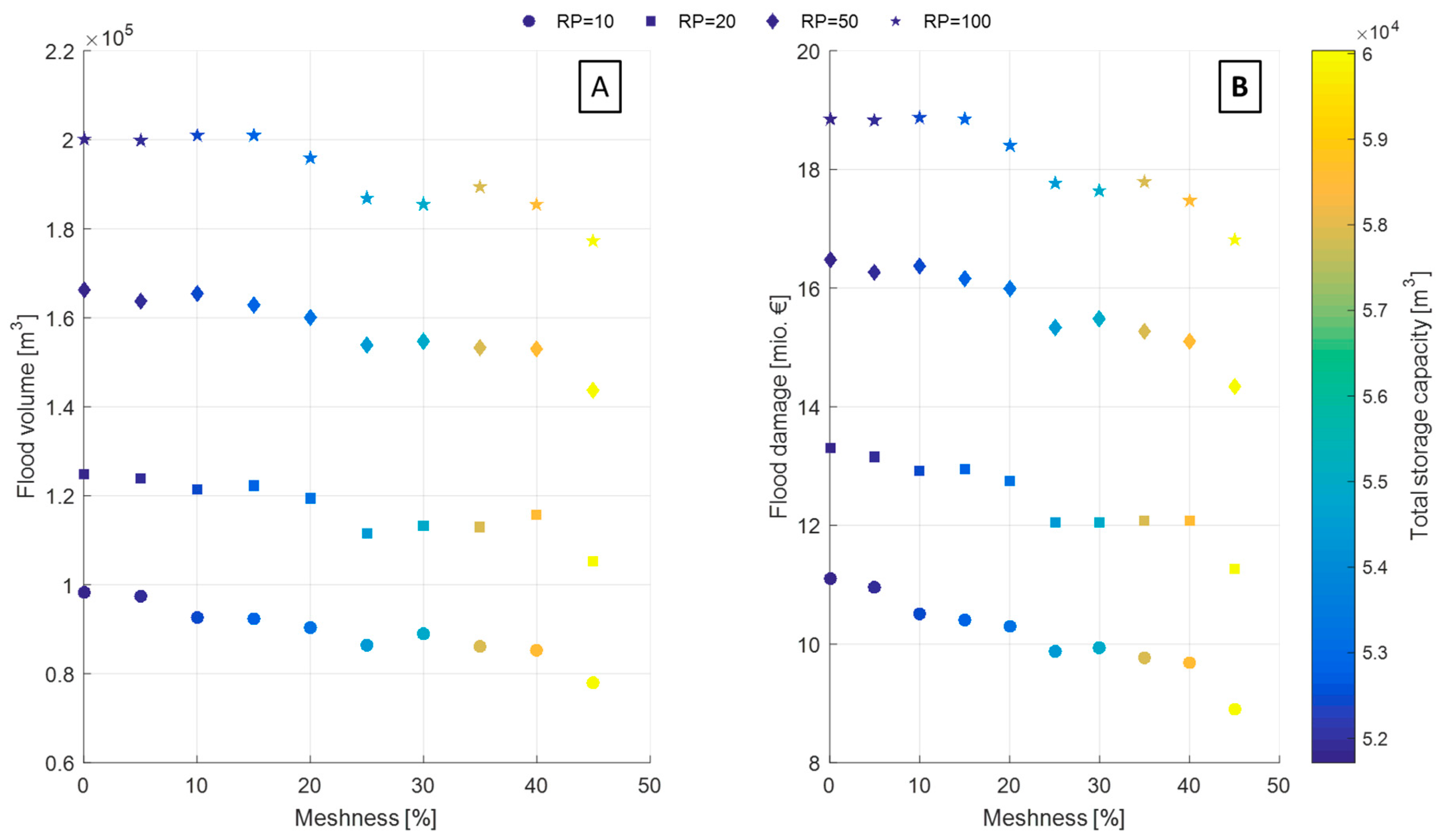
The relationship of Meshness with flood volumes and flood damage for the different rain events can be seen in Figure 2A,B, respectively. The results for flood volumes correspond to total flooded volume for each scenario under each rain event. This is obtained by summing the flood volume of each individual junction of the network. The results show that higher Meshness degrees are associated with higher storage capacity values. This is an expected result, since an increase in Meshness is only achieved by installing additional pipes and therefore increasing the available volume. Furthermore, the results also suggest that increasing Meshness leads to lower flood volumes. This outcome is consistent with what is presented by Reyes-Silva et al. [11], where the topology of network played an important role in the magnitude and occurrence of functional failures, in this case node flooding. The probable reason is that the presence of extra pipes for increasing Meshness resulted in additional storage volume capacity of the system, preventing the occurrence of a more accentuated urban flood. The stochastic addition and removal of conduits also provide a series of alternative flow paths, which may contribute to a better distribution of the stormwater and reduce the number of flooded junctions in the UDN for each rain event. Nevertheless, this remains to be tested.
The relationship between the cost of flood damage and Meshness for different rain events is similar to in the case of flood volumes, i.e., flood damages reduce with increasing Meshness and increasing storage capacity (Figure 2B). This is expected since the damages are directly related to the flood depths and hence to the flood volumes. The estimated monetary values of the flood damages depend highly on the flood damage curves that are used. Therefore, the obtained results should not be interpreted in terms of absolute monetary reduction, but rather on the relative reduction in damage as a function of Meshness. In fact, the results indicate that increasing Meshness from 0% to 45% leads to flood damage reduction between 11% and 20%. This reduction depends on the intensity of the evaluated rain event. For instance, highly intense events generate considerable amounts of runoff that cannot be handled even by the increase in storage resulting from the increase in Meshness. This leads to relatively small variations (less than 5%) in the flooded volumes and in flood damage.
3.2. Cost–Benefit Analysis
Table 1 summarizes the results obtained for the benefits calculation. All values are presented in terms of millions of euros (EUR 106) for the year 2019. For each Meshness scenario, the flood damage results for the different return periods are combined to obtain an expected annual flood damage, measured in millions of Euros per year. For more information on how these values are combined to obtain an expected annual flood damage values, see Appendix B. As seen before, an increase in Meshness is associated with a decrease in flood damage. For instance, by comparing the scenarios with the lowest (0%) and highest Meshness possible (45%), it can be seen that in the last case, the expected annual damages are reduced by almost 20%. Furthermore, the present values of the expected damages for the entire pipe life cycle are calculated by multiplying the expected annual values by 50 years (life expectancy of pipes) without considering inflation. Lastly, the incremental benefits of each scenario are calculated as the difference between the total expected damage of the 0% Meshness case and the total expected damages for the corresponding scenario. Benefits here represent the amount of euros that are not lost due to flood damage by increasing the Meshness in the system. As an example, increasing Meshness from 0% to 5% leads only to a reduction in the expected flood damages for the entire life expectancy of the sewer system of 2.03 million Euros, while increasing Meshness up to 45% leads to a saving of 32 million Euros due to avoiding flood damage.
Table 2 summarizes the results obtained for the costs calculation. All values are presented in terms of millions of Euros (EUR 106). The total investment for each scenario corresponds to the sum of the installation cost at the beginning of the project and the O&M cost during the life expectancy of the system. This value is obtained by multiplying the annual O&M fees by the pipe life expectancy (50 years) without considering inflation. Since an increase in Meshness can only be obtained by adding more pipes into the network, the total investment costs increase with higher Meshness degrees. In this context, costs are calculated as the difference between the total investments for the 0% Meshness case (i.e., the base conditions) and the total investments for the corresponding scenario. Costs thus represent the amount of additional money that needs to cover the installation and O&M of the additional pipes that lead to Meshness increments. As an example, for the 25% Meshness scenario, it is necessary to invest 7.33 million more for the initial installation and O&M of the system in comparison to the base scenario (0% Meshness).
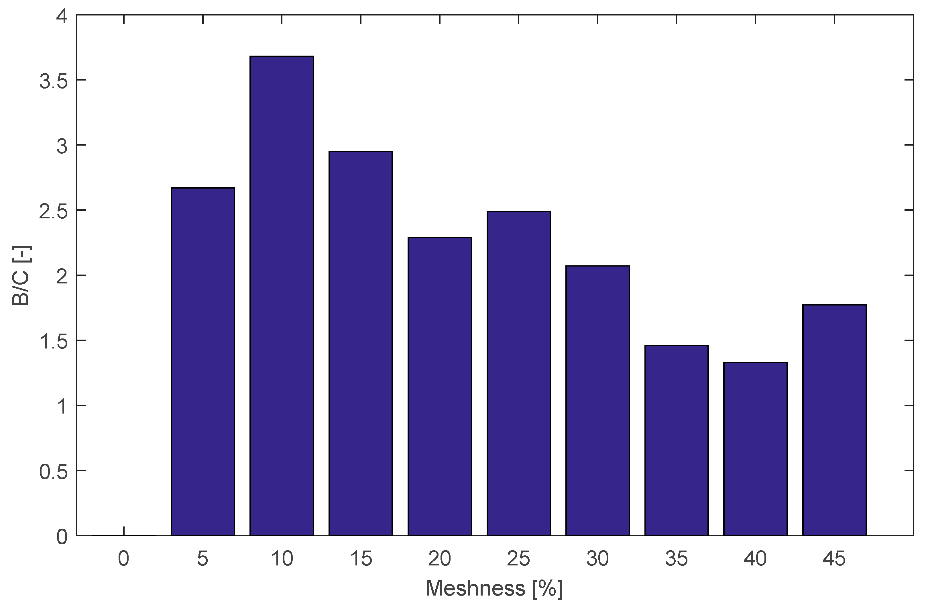
As mentioned before, the cost–benefit analysis determines the most appropriate layout which balances costs and benefits of increasing Meshness. This is done based on the absolute ratio (B/C) between benefits (B) and costs (C) for the entire pipe system life cycle. This ratio is calculated for each of the scenarios using the total incremental benefits and costs presented in Table 1 and Table 2, respectively. Figure 3 illustrates the B/C results obtained as a function of the different Meshness scenarios. No results are displayed for the scenario of 0% Meshness since it corresponds to the reference conditions for the cost–benefit calculations. The results suggest that all scenarios have an economic viability since the benefits are always higher than the costs (B/C > 1.0). This indicates that although adding more pipes than the minimum required, i.e., transitioning from a pure branched layout to a more meshed configuration, is associated with high pipe-related costs, the related benefits are always higher. Hence, increasing Meshness can be considered as a cost-effective solution, at least in terms of flood damage reduction for the analyzed Meshness range.
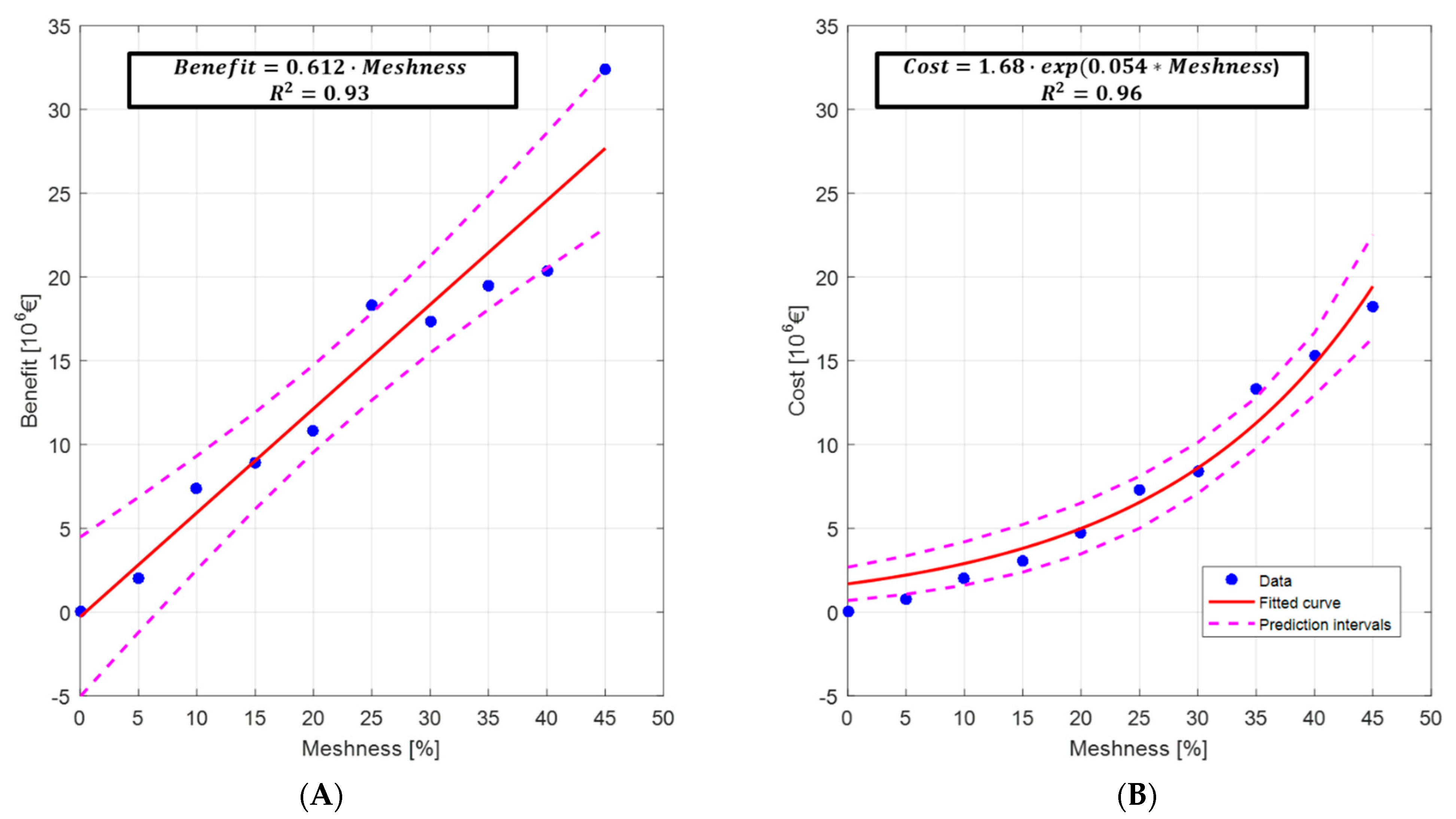
The B/C ratio, however, differs significantly among the different analyzed levels of Meshness. In fact, a maximum value of approximately 3.7 occurs at the 10% scenario. For higher Meshness values, the B/C values decrease gradually up to a minimum of 1.3, corresponding to the 40% Meshness case (Figure 3). Such behavior can be explained by the way in which benefits and costs change as a function of Meshness. Figure 4A,B illustrate these relationships, including the obtained regression equations for each case and 95% prediction intervals. On the one hand, the benefits, i.e., flood damage reductions, follow a linear trend. The values depicted in Figure 4A correspond to absolute values of the benefits presented in Table 1. Results suggest that the benefits increase rapidly as a function of Meshness, at an approximate rate of 0.612 × 10⁶ € per 1% increase in Meshness. On the other hand, increments of costs as a function of Meshness can be expressed with an exponential function (Figure 4B). Hence, for low Meshness values, costs increase at a slower rate than the benefits. As a consequence, the ratio between benefits and costs is higher for low Meshness values. This explains why the optimal B/C occurs in the 10% Meshness scenario and then decreases as Meshness increases. Considering this, it is hypothesized that there is a possible critical Meshness value which is economically unfeasible (B/C ratio below 1). This critical value should represent a network layout which is predominantly meshed, i.e., high Meshness and it is a cost-ineffective measure. Nevertheless, this remains to be tested.
4. Discussion
The structure of an urban drainage network can have a strong influence on the magnitude of pluvial urban flooding events. In fact, results from this study suggest that increasing Meshness tends to reduce flood volumes. Such effect is associated with the additional storage capacity added by the presence of extra pipes. Previous studies have also identified this link between the increasing capacity of the UDN due to the increasing Meshness, with pluvial urban flood reduction [11,12]. Furthermore, such studies suggest that adding extra pipes provides an increase in redundancy in the network, therefore increasing the resilience of the system [11]. As a consequence, the system is able to distribute wastewater flows along the network in a better way, reducing the hydraulic stress on the system and hence decreasing flood frequency. In this context, increasing Meshness can be considered as an effective solution for flood management that can be applied for optimizing existing networks or for the appropriate planning of future developments.
Efficiency of this approach, however, depends on the placement of additional pipes. On the one hand, although theoretically pipes can be added to reach a maximum of 100% Meshness, the resulting layout might not be realistic since it is not always feasible to install pipes everywhere in the catchment due to spatial constrains. Topographic conditions may limit the expansion of the system, therefore limiting the benefits related to increasing Meshness. In other words, a significant increment of Meshness degrees might not be achieved in every catchment due to topographic conditions that limit the implementation of additional pipes. Further studies should focus then on analyzing the potential flood reduction when combining changes in Meshness with other flood management practices. On the other hand, randomly adding pipes to the network might not be an efficient solution. In fact, previous studies have suggested that the expansion of the system should be done by maximizing the added storage capacity associated with pipe implementation [12,16]. It is recommended then that future studies should focus on identifying all the potential and optimal areas for Meshness expansion. In other words, studies should focus on analyzing all the sections of the network where it is spatially and technically feasible to install additional pipes while maximizing the added storage capacity to the system.
The presented results indicate that for all the analyzed scenarios, the benefits were consistently higher than the associated installation, O&M costs. This suggests that increasing Meshness is not only an effective measure in terms of urban pluvial flood volume reduction but is also cost-efficient and economically viable. These results, however, consider only the direct benefits of reducing tangible impacts related to urban flooding, i.e., damage to properties and their contents (see Section 2.5). In order to have an integral evaluation of the advantages of increasing Meshness, further benefits should be considered. For instance, urban flooding may have other indirect impacts such as business interruption, damaging critical infrastructure networks (e.g., roads, water supply or electrical grids) or even have severe impacts in terms of public health and environmental pollution [24]. In this context, reducing flood volumes by increasing Meshness may be associated with unquantified benefits.
The current approach aims to have a general view on the cost-efficiency of increasing Meshness as a measure for urban flood reduction and to illustrate a procedure for determining an optimal sewer network layout. It is expected that this approach can be used to analyze other existing urban systems or to support the design of new urban drainage networks. To do so, some improvements need to be done in order to adapt this approach and to have more accurate results for each specific location. Accordingly, besides the aforementioned consideration of additional benefits, further research should focus on defining more generalized methods to improve the estimation of the pipe installation costs. In fact, as it can be seen in Table 2, such costs represent the highest fraction of the total investments. Therefore, cost–benefit calculations are quite sensitive to the function used to estimate pipe installation expenses. In general, such functions relate costs as a function of the pipe’s material, diameter and excavation depth (see for example [22,25,26]). These functions, however, are case specific and therefore determining precise pipe installation costs for each location might be challenging. Hence, it is recommended that future studies should define functions that can be adapted to different local conditions.
5. Summary and Conclusions
The present work focused on analyzing how different structures of a single urban drainage network affected flood volumes and their associated damages. Furthermore, a cost–benefit analysis was used to determine the best network structure. As a case study, a sewer subnetwork in Dresden, Germany was selected. Structure was measured in terms of Meshness. This is a coefficient that can vary between 0% and 100%, representing layouts with the least number of pipes without causing any disconnection, and with the maximum number of connected pipes per inner node, respectively. Scenarios corresponding to Meshness values between 0% and 45% were developed and implemented in EPA SWMM. Scenarios were limited to 45% Meshness due to spatial restrictions. Event-wise simulations using design storms of 10, 20, 50 and 100 year return period were performed to obtain data regarding the characteristics of flood events. These results were coupled with a diffusive overland flow model to determine flood depths. This information was further used to calculate flood damage, according to depth-damage curves for Germany. Based on this, benefits were measured in terms of flood damage reduction, while costs corresponded to investments related to pipe installation, operation and maintenance.
Results suggested that an increment in Meshness was related to a decrease in flood volumes and therefore in flood damage. It was identified that the main cause of this was the increase in total sewer storage capacity associated with an increase in Meshness. Scenarios with a high Meshness degree were characterized by the presence of additional pipes which increased the total capacity of the system. This allowed a better distribution of flow, decreasing the hydraulic stress in the network and hence reducing the occurrence and magnitude of flood events.
Furthermore, outcomes of the cost–benefit analysis indicated that all analyzed scenarios were identified as cost-effective. This meant that for all the analyzed levels of Meshness, the benefits were consistently higher than costs. In fact, the ratios between benefits and costs (B/C) were higher than 1 for all scenarios, thus indicating that increasing Meshness leads to a decrease in flood damage that is consistently higher than the investments needed to achieve such network structure. Nevertheless, the B/C ratio varied significantly among the different analyzed levels of Meshness. In fact, clear maximum and minimum values were identified for the 10% and 40% Meshness scenarios, respectively. It is hypothesized that such behavior could be explained by the way in which both benefits and costs change as a function of Meshness. On the one hand, benefits increased rapidly with Meshness following a linear trend. On the other hand, the relationship between costs and Meshness followed an exponential behavior. For low Meshness values, costs increased at a slower rate than the benefits, thus leading to a higher B/C ratio. This explained why the optimal B/C occurred in the 10% scenario and then decreased as Meshness increased.
Increasing Meshness can be classified as a cost-effective measure for urban flood reduction. Nevertheless, implementation of such an approach depends on the topographic conditions of the intervention area. In fact, local characteristics may limit the installation of additional pipes. In order to increase the efficiency of this approach given other local spatial restrictions, it is suggested that future studies should focus on the identification of optimal locations where it is spatially and technically feasible to install additional pipes while maximizing the storage capacity added to the system. It is hypothesized that the efficiency of this approach can be improved by integrating it with other urban flood management strategies, such as the implementation of green infrastructures.
The effects of the physical arrangement, i.e., the layout, of sewer networks on the occurrence and magnitude of pluvial flood events is still not fully understood and investigated. In this context, the results obtained in this study are expected to build a basis for future analyses, and to illustrate the potential of increasing Meshness as a cost-efficient measure for urban flood reduction. Here, a procedure for determining an optimal sewer network layout was proposed using as an example a real case study. The results from this type of approach could serve as a support for the better design, management and operation of urban drainage networks. Additionally, it is expected that the current approach and results obtained from it could be a basis for developing a new structural resilience analysis based mainly on the sewer network layout.
Author Contributions
Conceptualization, J.D.R.-S. and B.H.; methodology, J.D.R.-S.; software, A.C.N.B.F. and J.D.R.-S.; formal analysis, J.D.R.-S. and K.L.R.-G.; investigation, J.D.R.-S. and K.L.R.-G.; data curation, A.C.N.B.F.; writing—original draft preparation, A.C.N.B.F. and J.D.R.-S.; writing—review and editing, J.D.R.-S.; visualization, J.D.R.-S.; supervision, P.K.; funding acquisition, P.K. All authors have read and agreed to the published version of the manuscript.
Funding
This work was supported by the Excellence Initiative of the German Federal and State Governments, through the of the International Research Training Group ‘Resilient Complex Water Networks’ (PSP F-003661-553-A5E-1180101). Open Access Funding by the Publication Fund of the TU Dresden.
Institutional Review Board Statement
Not applicable.
Informed Consent Statement
Not applicable.
Data Availability Statement
The data presented in this study is available on request from the corresponding author.
Acknowledgments
The presented work was conducted under the framework of the International Research Training Group ‘Resilient Complex Water Networks’. It is supported by TU Dresden’s Institutional Strategy. TU Dresden’s Institutional Strategy is funded by the Excellence Initiative of the German Federal and State Governments. The IRTG is a joint initiative of TU Dresden, Helmholtz-Centre for Environmental Research (UFZ) with their Center of Advanced Water Research (CAWR), Purdue University (USA) and University of Florida (USA). The authors gratefully acknowledge the cooperation with the Stadentwässerung Dresden GmbH.
Conflicts of Interest
The authors declare no conflict of interest.
Appendix A
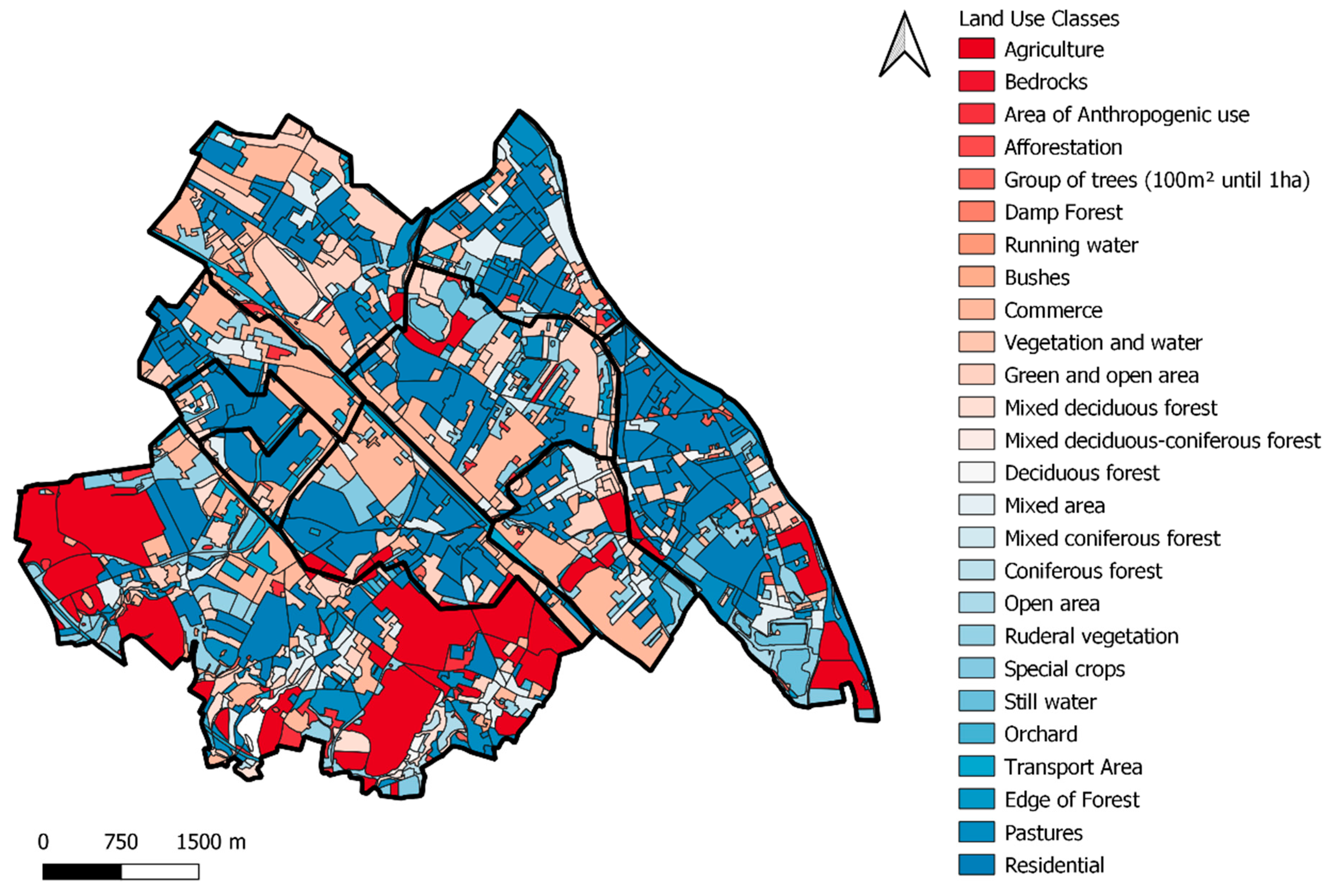
The local authorities have identified 28 different land use classes in the area—see Figure A1. Nevertheless, in order to perform the desired flood damage analyses, such categories needed to be reclassified into six different new land use classes: Agriculture, Industry, Commerce, Residential, Infrastructure and No Damage. The results of this reclassification can be seen in Table A1 and Figure A2.

Table A1.
Categories for land use reclassification.
| Original Land Use | Reclassified Land Use |
|---|---|
| Mixed area | 50% Residential area + 50% Commercial |
| Agriculture | Agriculture |
| Special crops | |
| Orchard | |
| Economic grassland | |
| Commercial area/technical infrastructure | Commercial |
| Anthropogenic used special areas (excavation area, storage...) | Industry |
| Field wood/group of trees (dense/closed), 100 m to 1 ha | Infrastructure |
| Bushes | |
| Green and open spaces | |
| Traffic areas | |
| Bedrocks | No Damage |
| Afforestation | |
| Damp forest | |
| Running water | |
| Vegetation accompanying the water | |
| Mixed deciduous forest | |
| Foliage-coniferous mixed forest | |
| Deciduous forest (pure stock) | |
| Mixed coniferous forest | |
| Coniferous forest (pure stock) | |
| Open areas | |
| Ruderal corridor, perennial corridor | |
| Still waters | |
| Forest edge areas/pre-forests | |
| Residential area | Residential area |
Figure A1.
Land use classes in the study area (adapted from [13]).
Figure A1.
Land use classes in the study area (adapted from [13]).

Figure A2.
Reclassified land uses.

Appendix B
The expected annual flood damage value for each Meshness scenario is determined using the flood damage results obtained for each analyzed rainfall event. This is done following the guidelines proposed by the Ministry for Environment, Climate and Energy Management of Baden-Württemberg (Ministerium für Umwelt, Klima und Energiewirtschaft) [23]. Table A2 exemplifies this process based on the results for the 0% Meshness scenario. Besides the four return periods analyzed (10, 20, 50 and 100) and their associated results, data from a 2-year return period, the design event, and a hypothetical event with low probability, i.e., a return period close to infinity, are included. It is assumed that no flood occurs for the 2-year event since it is the design storm and therefore no damages are associated with it. Moreover, it is also assumed that the damages associated with events with low probability, i.e., return periods higher than 100 years, are similar to those of the lowest analyzed probability (0.01). The column “Δ Probability” is a calculation column in which the difference between the probability of occurrence between the upper and lower grid points of the different intervals. This is multiplied by the mean value of the damage in the interval for the damage expectation of the interval. The sum over all intervals corresponds to the expected damage per year, which in this case is 3.64 106 EUR/year. Similar procedures were done to obtain the expected annual damage values for the other Meshness scenarios.
Table A2.
Expected annual flood damage calculation matrix for the 0% Meshness scenario.
| Interval | Return Period [Year] | Probability [-] | Δ Probability [-] | Damage [106 EUR] | Mean Damage [106 EUR] | Expected Damage per Year [106 EUR/Year] |
|---|---|---|---|---|---|---|
| 2 | 0.5 | 0 | ||||
| 1 | 0.4 | 5.55 | 2.22 | |||
| 10 | 0.1 | 11.09 | ||||
| 2 | 0.05 | 12.20 | 0.61 | |||
| 20 | 0.05 | 13.30 | ||||
| 3 | 0.03 | 14.89 | 0.45 | |||
| 50 | 0.02 | 16.48 | ||||
| 4 | 0.01 | 17.66 | 0.18 | |||
| 100 | 0.01 | 18.84 | ||||
| 5 | 0.01 | 18.84 | 0.19 | |||
| ∞ | 0 | 18.84 |
References
- Shuster, W.D.; Bonta, J.; Thurston, H.; Warnemuende, E.; Smith, D.R. Impacts of impervious surface on watershed hydrology: A review. Urban Water J. 2005, 2, 263–275. [Google Scholar] [CrossRef]
- Burns, M.J.; Fletcher, T.D.; Walsh, C.J.; Ladson, T.; Hatt, B. Hydrologic shortcomings of conventional urban stormwater management and opportunities for reform. Lands. Urban Plan. 2012, 105, 230–240. [Google Scholar] [CrossRef]
- Arns, S.; Hellmig, M. Effects of Heavy Rainfall on Construction-Related Infrastructure; Federal Institute for Research on Building, Urban Affairs and Spatial Development (BBSR): Berlin, Germany, 2018. [Google Scholar]
- Butler, D.; Digman, C.; Makropoulos, C.; Davies, J.W. Urban Drainage, 4th ed.; Taylor and Francis Group: Boca Raton, FL, USA, 2018. [Google Scholar]
- Jiang, Y.; Zevenbergen, C.; Ma, Y. Urban pluvial flooding and stormwater management: A contemporary review of China’s challenges and “sponge cities” strategy. Environ. Sci. Policy 2018, 80, 132–143. [Google Scholar] [CrossRef]
- Lee, J.; Chung, G.; Park, H.; Park, I. Evaluation of the Structure of Urban Stormwater Pipe Network Using Drainage Density. Water 2018, 10, 1444. [Google Scholar] [CrossRef] [Green Version]
- GebreEgziabher, M.; Demissie, Y. Modeling Urban Flood Inundation and Recession Impacted by Manholes. Water 2020, 12, 1160. [Google Scholar] [CrossRef] [Green Version]
- Bhattarai, R.; Yoshimura, K.; Seto, S.; Nakamura, S.; Oki, T. Statistical model for economic damage from pluvial floods in Japan using rainfall data and socioeconomic parameters. Nat. Hazards Earth Syst. Sci. 2016, 16, 1063–1077. [Google Scholar] [CrossRef] [Green Version]
- Petrucci, O.; Aceto, L.; Bianchi, C.; Bigot, V.; Brazdil, R.; Pereira, S.; Kahraman, A.; Kilic, O.; Kotroni, V.; Llasat, M.C.; et al. Flood Fatalities in Europe, 1980–2018: Variability, Features, and Lessons to Learn. Water 2018, 11, 1682. [Google Scholar] [CrossRef] [Green Version]
- Zhang, C.; Wang, Y.; Li, Y.; Ding, W. Vulnerability Analysis of Urban Drainage Systems: Tree vs. Loop Networks. Sustainability 2017, 9, 397. [Google Scholar] [CrossRef] [Green Version]
- Reyes-Silva, J.D.; Helm, B.; Krebs, P. Meshness of sewer networks and its implications for flooding occurrence. Water Sci. Technol. 2020, 81, 40–51. [Google Scholar] [CrossRef] [PubMed]
- Hesarkazzazi, S.; Hajibabaei, M.; Reyes-Silva, J.D.; Krebs, P.; Sitzenfrei, R. Assessing Redundancy in Stormwater Structures under Hydraulic Design. Water 2020, 12, 1003. [Google Scholar] [CrossRef] [Green Version]
- Landesamt fur Umwelt, Landwirtschaft und Geologie. iDA—Interdisziplinäre Daten und Auswertunge. 2020. Available online: https://www.umwelt.sachsen.de/umwelt/infosysteme/ida/ (accessed on 15 May 2020).
- Huizinga, J.; de Moel, H.; Szewczyk, W. Global Flood Depth-Damage Functions: Methodology and the Database with Guidelines; EUR 28552 EN; European Union: Luxembourg, 2017. [Google Scholar]
- Kruskal, J.B. On the shortest spanning subtree of a graph and the traveling salesman problem. Proc. Am. Math. Soc. 1956, 7, 48–50. [Google Scholar] [CrossRef]
- Reyes-Silva, J.; Bangura, E.; Helm, B.; Benisch, J.; Krebs, P. The Role of Sewer Network Structure on the Occurrence and Magnitude of Combined Sewer Overflows (CSOs). Water 2020, 12, 2675. [Google Scholar] [CrossRef]
- Rossman, L.A. Storm Water Management Model, User’s Manual, Version 5.1; EPA: Cincinnati, OH, USA, 2015.
- Abwasser und Abfall e.V. DWA Deutsche Vereinigung fur Wasserwirtschaft. Arbeitsblatt DWA-A 118 Hydraulische Bemessung und Nachweis Hydraulische Bemessung und Nachweis; Abwasser und Abfall e.V. DWA Deutsche Vereinigung fur Wasserwirtschaft: Hennef, Germany, 2006. [Google Scholar]
- Junghaenel, T.; Ertel, H.; Deutschländer, T. Bericht zur Revision der Koordinierten Starkregen Regionalisierung und -Auswertung des Deutschen Wetterdienstes in der Version 2010; Offenbach am Main: Deutscher Wetterdienst Abteilung Hydrometeorologie: Berlin, Germany, 2017. [Google Scholar]
- Chen, W.; Huang, G.; Zhang, H. Urban stormwater inundation simulation based on SWMM and diffusive overland-flow model. Water Sci. Technol. 2017, 76, 3392–3403. [Google Scholar] [CrossRef] [PubMed]
- World Bank. Consumer Price Index—Germany; World Bank: Washington, DC, USA, 2019; Available online: https://data.worldbank.org/indicator/FP.CPI.TOTL?end=2019&locations=DE&start=2010 (accessed on 14 April 2020).
- Freistaat Thüringen. Regelungen zur Aufstellung von Abwasserbeseitigungskonzepten; Thüringer Ministerium für Umwelt, Energie und Naturschutz: Erfurt, Germany, 2005. Available online: https://umwelt.thueringen.de/themen/boden-wasser-luft-und-laerm/abwasserentsorgung-u-wassergefaehrdende-stoffe/abwasserbeseitigungskonzepte (accessed on 15 October 2020).
- Zeisler, P.; Pflügner, W. Hochwasser Risikomanagement Baden-Württemberg; Landes Baden-Württemberg: Baden-Württemberg, Germany, 2019; Available online: https://www.hochwasser.baden-wuerttemberg.de/documents/43970/44031/HWS-BW-Arbeitshilfe_Teile_I_und_II_20190122_V01_0_Druckfassung.pdf (accessed on 10 October 2020).
- Hammond, M.J.; Chen, A.S.; Djordjevic, S.; Butler, D.; Mark, O. Urban flood impact assessment: A state-of-the-art review. Urban Water J. 2015, 12, 14–29. [Google Scholar] [CrossRef] [Green Version]
- Maurer, M.; Wolfram, M.; Anja, H. Factors affecting economies of scale in combined sewer systems. Water Sci. Technol. 2010, 62, 36–41. [Google Scholar] [CrossRef] [PubMed]
- Marchionni, V.; Lopes, N.; Mamouros, L.; Covas, D. Modelling Sewer Systems Costs with Multiple Linear Regression. Water Resour. Manag. 2014, 28, 4415–4431. [Google Scholar] [CrossRef]
Figure 1.
Urban drainage network (UDN) and catchment in the study area.

Figure 2.
Flood volumes (A) and flood damages (B) for the different rain events as a function of Meshness, including the total storage capacity of the system for each analyzed Meshness degree.
Figure 2.
Flood volumes (A) and flood damages (B) for the different rain events as a function of Meshness, including the total storage capacity of the system for each analyzed Meshness degree.

Figure 3.
Ratio between benefits (B) and costs (C) for different Meshness degrees.

Figure 4.
Regressions between benefits (A) and costs (B) as a function of Meshness. Including fitted lines, their 95% prediction interval (red and magenta lines, respectively).
Figure 4.
Regressions between benefits (A) and costs (B) as a function of Meshness. Including fitted lines, their 95% prediction interval (red and magenta lines, respectively).

Table 1.
Benefits of increasing Meshness in the UDN (Present value in euros 2019). Negative values represent savings due to avoiding flood damage.
Table 1.
Benefits of increasing Meshness in the UDN (Present value in euros 2019). Negative values represent savings due to avoiding flood damage.
| Meshness [%] | Expected Flood Damage per Year [ 106 €/Year] | Flood Damages in Life Expectancy of 50 Years [106 €] | Total Incremental Benefits [106 €] |
|---|---|---|---|
| 0 | 3.64 | 182.00 | - |
| 5 | 3.60 | 179.97 | −2.03 |
| 10 | 3.49 | 174.60 | −7.39 |
| 15 | 3.46 | 173.06 | −8.94 |
| 20 | 3.42 | 171.17 | −10.82 |
| 25 | 3.27 | 163.72 | −18.28 |
| 30 | 3.29 | 164.66 | −17.34 |
| 35 | 3.25 | 162.54 | −19.45 |
| 40 | 3.23 | 161.64 | −20.35 |
| 45 | 2.99 | 149.63 | −32.37 |
Table 2.
Costs of increasing Meshness in the UDN (Present value in euros 2019).
| Meshness [%] | Installation [106 €] | O&M [106 €/Year] | O&M in Life Expectancy of 50 Years [106 €] | Total Investment [106 €] | Total Incremental Costs [106 €] |
|---|---|---|---|---|---|
| 0 | 81.05 | 0.227 | 11.35 | 92.41 | - |
| 5 | 81.69 | 0.230 | 11.48 | 93.17 | 0.76 |
| 10 | 82.78 | 0.233 | 11.64 | 94.42 | 2.01 |
| 15 | 83.66 | 0.236 | 11.78 | 95.44 | 3.03 |
| 20 | 85.10 | 0.241 | 12.03 | 97.13 | 4.72 |
| 25 | 87.36 | 0.247 | 12.37 | 99.73 | 7.33 |
| 30 | 88.28 | 0.250 | 12.51 | 100.79 | 8.38 |
| 35 | 92.68 | 0.261 | 13.06 | 105.74 | 13.33 |
| 40 | 94.33 | 0.267 | 13.37 | 107.71 | 15.30 |
| 45 | 96.90 | 0.275 | 13.74 | 110.64 | 18.24 |
Publisher’s Note: MDPI stays neutral with regard to jurisdictional claims in published maps and institutional affiliations. |
© 2021 by the authors. Licensee MDPI, Basel, Switzerland. This article is an open access article distributed under the terms and conditions of the Creative Commons Attribution (CC BY) license (https://creativecommons.org/licenses/by/4.0/).
Share and Cite
MDPI and ACS Style
Reyes-Silva, J.D.; Frauches, A.C.N.B.; Rojas-Gómez, K.L.; Helm, B.; Krebs, P. Determination of Optimal Meshness of Sewer Network Based on a Cost—Benefit Analysis. Water 2021, 13, 1090. https://doi.org/10.3390/w13081090
AMA Style
Reyes-Silva JD, Frauches ACNB, Rojas-Gómez KL, Helm B, Krebs P. Determination of Optimal Meshness of Sewer Network Based on a Cost—Benefit Analysis. Water. 2021; 13(8):1090. https://doi.org/10.3390/w13081090
Chicago/Turabian StyleReyes-Silva, Julian D., Ana C.N.B. Frauches, Karen L. Rojas-Gómez, Björn Helm, and Peter Krebs. 2021. "Determination of Optimal Meshness of Sewer Network Based on a Cost—Benefit Analysis" Water 13, no. 8: 1090. https://doi.org/10.3390/w13081090
Note that from the first issue of 2016, this journal uses article numbers instead of page numbers. See further details here.