
Influence of Community Factors on Water Saving in a Mega City after Implementing the Progressive Price Schemes

1
School of Environmental and Chemical Engineering, Shanghai University, Shanghai 200444, China
2
School of Economics, Shanghai University, Shanghai 200444, China
3
Shanghai Water Supply Management Office, Shanghai 200081, China
*
Authors to whom correspondence should be addressed.
Water 2021, 13(8), 1097; https://doi.org/10.3390/w13081097
Submission received: 2 March 2021
/
Revised: 2 April 2021
/
Accepted: 13 April 2021
/
Published: 16 April 2021
(This article belongs to the Section Water Resources Management, Policy and Governance)
Abstract
:A progressive price scheme (PPS) has been implemented in Shanghai since 2013 in consideration of residents’ ability to pay, and charges are based on the actual water consumption of the residents, in an effort to balance the rational allocation of water resources and the goal of saving water between rich and poor families. In the current work, the effect of the PPS for water use was evaluated based on the water use of 6661 households from 14 communities in Shanghai. It was found that the PPS did not reduce household water consumption when comparing the water consumption per household both before and after the implementation of the PPS policy. To investigate the weakness of the PPS, a principal component analysis (PCA) and a hierarchical cluster analysis (HCA) were conducted to access the relationships between mean household water use and community factors such as housing price, management fees, and the number of parking sites. Moreover, a significant inverted U-shaped curve between housing price and water use was found, which demonstrates that rental households shared by several tenants were the main consumers of residential water, and they were not sensitive to the water price improvement in the PPS due to sharing water prices. Therefore, a proposal was made in this work to increase the proportion of water fee expenditure in the total household income and to use 3% as the benchmark for water affordability. Our results provided a new picture of residential water use in big cities and a method for saving and balancing urban water resources.
1. Introduction
Water is a precious and strategic resource that is important in the development of society and the economy [1,2]. Residential water consumption accounts for a large percentage of the total water consumption in the urban water system [3,4]. According to the European Environment Agency, 130–150 L/day per capita of drinking water is used by an average European citizen [5]. The authors in [6] reported a 333 L/day per capita water consumption in Texas, USA. In London, the average water consumption is about 600 L/day per capita [7], while in Spain, the average annual per capita water consumption is 43 m3, representing an average of 118 L/day per capita [8]. The living water consumption of urban residents in Shenzhen, China, is 166 L/day per capita [9]. In 2014, China’s 38 major cities had an average water consumption of 129 L/day per capita [10]. Per capita domestic water consumption in China is close to that of European countries. This level of consumption does not seem to be a problem. However, in China’s megacities, where there is a large residential population, the water consumption is many times that of European cities. The management of residential water is always a challenge for city administrators because of the increasing urban population and shortage of water resources [11,12]. In addition, residential water use behavior is always complex and hard to quantify. Accordingly, before establishing a complete management system for urban water resources, a study of residential water use is essential.
Urban residential water use has been investigated since the 1960s [13]. With the development of society and the economy, studies of residential water use began to focus on the internal mechanisms of household water use, and the effects of water prices, climate factors, and the characteristics of family members were studied widely [14]. The influence of water prices on residential water consumption is complicated [15]. Zheng and Kamal [16] found that an increase in price increases causes a decrease in household water consumption. Domestic water demand responds more strongly to price increases than to price drops [17]. Low-income households are more sensitive to water prices than high-income households. Water prices have different effects on residential water use for different purposes. For instance, water consumption for drinking and cooking was shown to be insensitive to price change, whereas water consumption for car washing and gardening was restricted dramatically by high water prices [18,19]. Climate factors affect residential water use through temperature change and rainfall [20]. Changes in temperature can affect home gardening, drinking water, and bathing, whereas precipitation affects the amount of water used for keeping the environment clean and for washing cars [10]. Family composition (taking into consideration the number of family members and the age of each member) is the critical factor that influences household water consumption [21]. Family scale (the number of family members) was found to be the most decisive factor for household water consumption [22]. The method of residential water consumption based on IUMAT (Integrated Urban Metabolism Analysis Tool) modeling shows that, every extra family member is linked to a 95 L/day increase in water consumption [23]. The age of family members also has a great effect on household water consumption. Long duration and high frequency of showering usually occur in households containing teenagers, young men, and children [24], leading to higher water consumption in such households. Rajeevan and Mishra [21] found that households composed of two young people (average age <40 years old) had the largest water consumption. Conversely, households composed of older people had less water consumption due to their customary behavior.
For this, many countries have adopted different water charging policies. The price of water in Oman is administered in a two-block structure, and residential water demand is managed by revising water prices and reforming residential water subsidies [20]. The French are a successful example in their implementation of the polluter pays principle (PPP), i.e., paying fees based on the ratio of the amount of fresh water volume abstracted from the aquatic environment and to the wastewater discharged in river; the collected money is returned to water users who are willing to invest in improving the environment [25,26]. Beijing and Shanghai are representative cities in China with a large permanent population. In 2016, Beijing’s water consumption was 490 L/day per capita, whereas Shanghai’s water consumption reached 1189 L/day per capita. Beijing is located in Northern China, where water resources are relatively scarce, and water use behavior is affected significantly by the individual differences of residential water-consuming and water-saving behavior as well as the characteristics and differences in water saving and water consumption habits in different regions [27]. Shanghai is the economic center of China, with a high population density and a large demand for water resources. From 2000, the residential water price (RWP) in Shanghai was 1.51 CNY/m3 (the conversion exchange rate is about 6.5 CNY to 1 USD). In 2009, the RWP increased to 2.30 CNY/m3. At that time, due to low water prices and weak management, residents had a generally weak awareness of water conservation, and residential water consumption was still high [28,29]. Additionally, water departments enacted a higher cost for cleaner water, and this could not be reflected by RWP. Accordingly, for the purpose of reasonable water resource distribution and water saving, a progressive pricing scheme (PPS) for water use was implemented in Shanghai in September 2013. Compared to a direct increase in the water price, the PPS considers the different economic situations of residents, and it is easier to both accept and implement.
This study evaluates the effect of the PPS on the water use of 6661 households from 14 communities in Shanghai. The distribution of water consumption in different communities in Shanghai area and the water consumption both before and after the PPS was implemented are investigated. In this work, water consumption is considered in the context of a relative community (i.e., a large residential area with a relatively independent living environment in a certain area of the city and is equipped with a complete set of life service facilities, such as commercial outlets, schools, etc.); through a principal component analysis (PCA), household water use is connected to the community parameters of housing price, plot ratio, management fee and parking. To further investigate the differences and similarities between the communities in terms of household water use, housing price, and housing quality, we perform a hierarchical cluster analysis (HCA). Based on the results of the PPS evaluation and the statistical analyses for the household water use in the 14 communities, we propose a water price policy. Our study provides a new picture of urban household water use and a reference for water saving in modern big cities with different household characteristics.
2. Material and Methods
2.1. Data Collection
Data of the water use every two months of 6661 households in 14 communities during 2011–2017 were provided by Shanghai Chengtou Water Group Co., Ltd. (Shanghai, China), the company in charge of providing water services in Shanghai. The water use data were based on the household units and were collected in the form of manual meter reading in January, March, May, July, September, and November each year. In Table S1, the average monthly water consumption of 14 communities from 2011 to 2017 and the average monthly water consumption before and after the implementation of the PPS are listed.
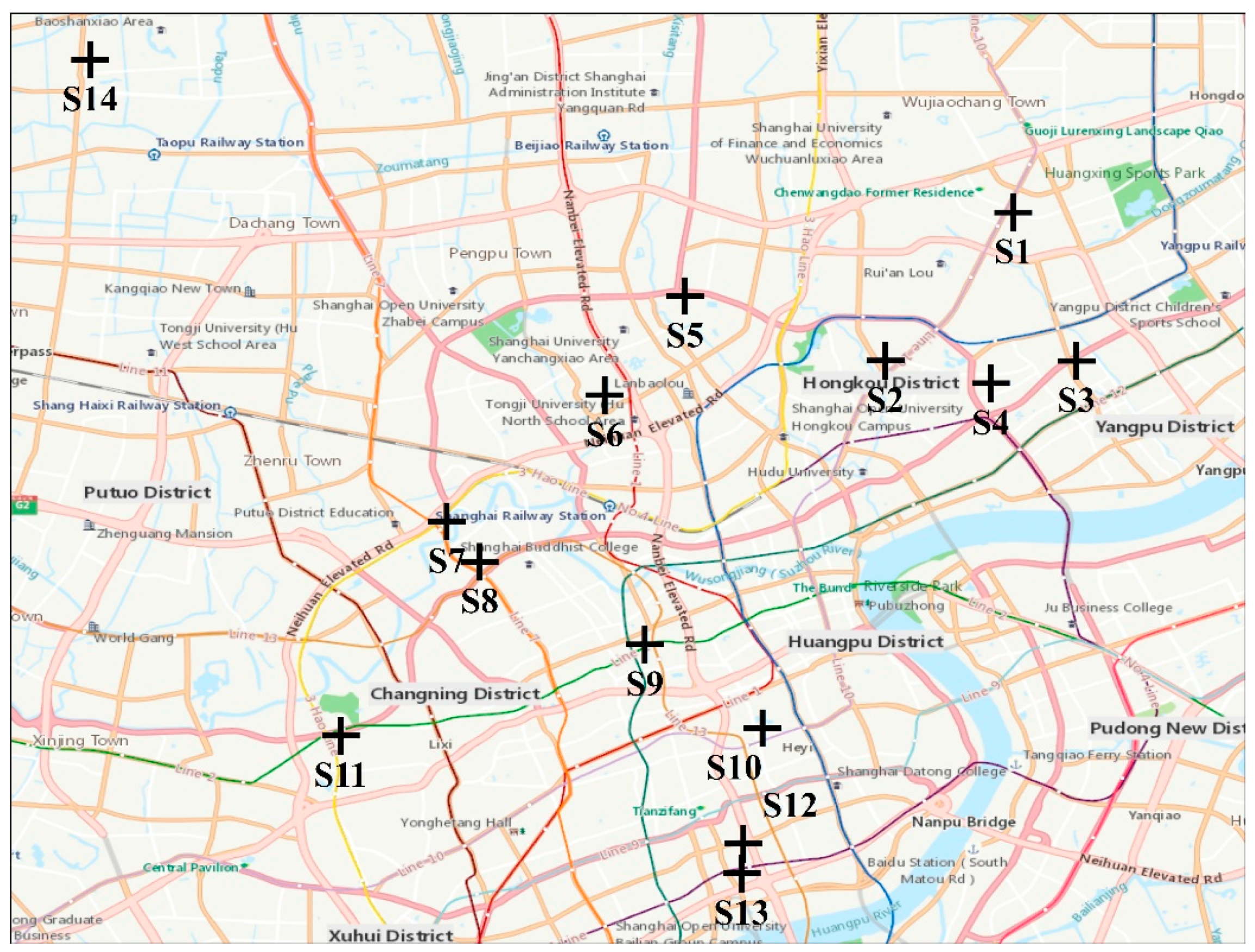
The 14 communities investigated were Linlvjiayuan (S1), Huahonggongyu (S2), Yangmingxincheng (S3), Haishanghai (S4), Baohuachengshihuayuan (S5), Shengyuanjiahaocheng (S6), Taixinjiayuan (S7), Shangqingjiayuan (S8), Jingansijiyuan (S9), Cuihutiandiyuan (S10), Kaixinghaoyuan (S11), Haiyuehuayuan (S12), Nanyuanxincun (S13), and Qiliansancun (S14), as shown in Figure 1. The 14 communities are the model communities for the implementation of the PPS. According to geographical location and housing price, they were divided into high-end, mid-range, and low-end communities. Of these, S9 and S10 are upscale communities due to their great location, and S13 and S14 are typical old communities.
Table 1 shows the abbreviations and descriptions of the 9 community indexes, including housing price, age of the building (until 2017), plot ratio, management fees, total number of households, number of parking sites, number of parking sites per household, green area ratio, and the ratio of unoccupied houses on the rental market to the total number of households. All the original community indices were collected from the estate website of Anjuke (https://shanghai.anjuke.com/, accessed on 8 January 2018). In addition, it also includes the average water consumption per household, which is the total water consumption of the community divided by the total number of occupied houses in the community. Thus, when these were combined with the household water use, a data matrix with 10 column vectors and 14 row vectors was established. We considered ethical factors involved and then created a description for each.
2.2. PPS in Shanghai
Since September 2013, Shanghai has formally implemented the PPS for residents in the municipal water supply and drainage service areas. The PPS is a common name for the implementation of classified metering charges and the over-quota progressive increase system or regressive price reduction system for the use of tap water. The PPS divides the water price into two or more sections. Each section has a unit water price that remains unchanged, and the unit water price increases in water consumption.
In the PPS, the water prices for the households with annual water use below 220 m3, between 220 and 300 m3, and over 300 m3 are 3.45, 4.83, and 5.83 CNY/m3, respectively. This price is a comprehensive water price that includes the price of tap water and the price of sewage treatment. The sewage treatment price is 1.70 CNY/m3, and the actual price is 1.53 CNY/m3 based on 90% of the drainage volume.
2.3. Statistical Analysis
A two-tailed Analysis of Variance (ANOVA) test was performed to compare the differences of mean values in this study. The significance level was accepted as the p value being less than 0.05.
A PCA was conducted to access the structure of the established matrix. PCA is a common method for dimension reduction [30]. The variables used are price, age, green%, MF, parking, water, ToHouse, PR, and CPH. The data period of water is from March 2011 to January 2017; the others are from 2011 to 2017. The correlation matrix of these variables is provided in the Table S2. The variables in the dataset were reduced into several noncorrelation components called principal components (PCs), which represented the linear weighted combination of the original variables (Equation (1)). Here, X and β represent the observed variable and weight, respectively. Each variable has its own loading on each PC. Thus, the relationships between the variables or samples can be accessed and visualized in either two or three dimensions. In this study, the number of PCs was determined by the scree plot.
The cluster analysis is an inductive method for data that aims to reveal the subsets of the observations in a dataset [31]. In this study, due to the small sample size, an HCA with average linkage was used to divide the communities into several clusters and to explain how the optimal number of clusters was determined in the HCA in Figure S1. According to the selected indices, observations with a high similarity were collected in a cluster. This step was repeated until all the samples were in one cluster. The similarity between samples was measured through Euclidean distance (Equation (2)). Here, i and j represent the observation values of i and j, respectively, and p means the number of variables.
A flowchart is added to the Supplementary Material to show the research methodology (Figure S2). All the analyses were conducted using the packages psych, Nbclust, and agricolae in R version 3.6.0 (https://www.r-project.org/, accessed on 6 May 2019).
3. Results and Discussion
3.1. Overview of the Dataset
3.1.1. Parameters of the 14 Investigated Communities
Table 2 shows the 14 communities’ indices in 2017. As shown in Table 2, the S9 and S10 communities have high housing prices, high MF, and high WL, which have a lot to do with their excellent geographical locations; these are all traits that belong to high-end communities. In contrast, the houses in the S13 and S14 communities are old, with low housing prices, low MF, and low WL, which are traits of typical low-end communities.
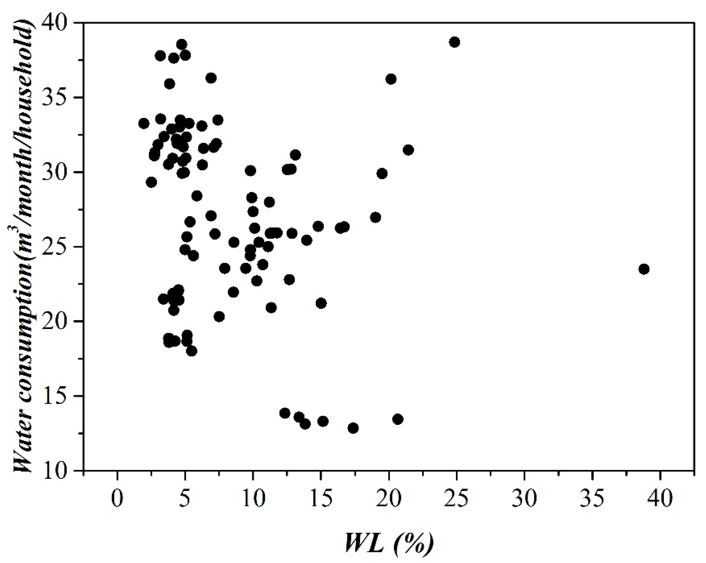
3.1.2. Relationship between the Number of Residents and Water Consumption
The relationship between the number of community residents and water consumption was examined by using the annual average water consumption and WL of each community from 2011 to 2017. Figure 2 shows that there is no significant relationship between the WL and water consumption, that is, the number of community residents does not affect water consumption. When the community has a large population, water consumption does not increase; when the number of residents decreases, water consumption does not decrease significantly.
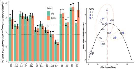
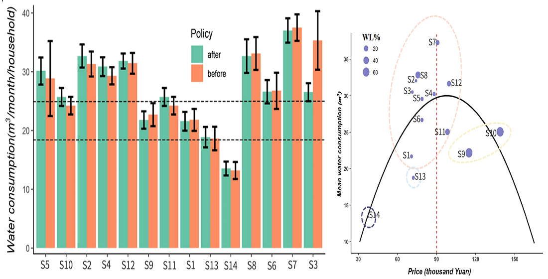
3.1.3. Changes in Water Consumption before and after PPS Implementation
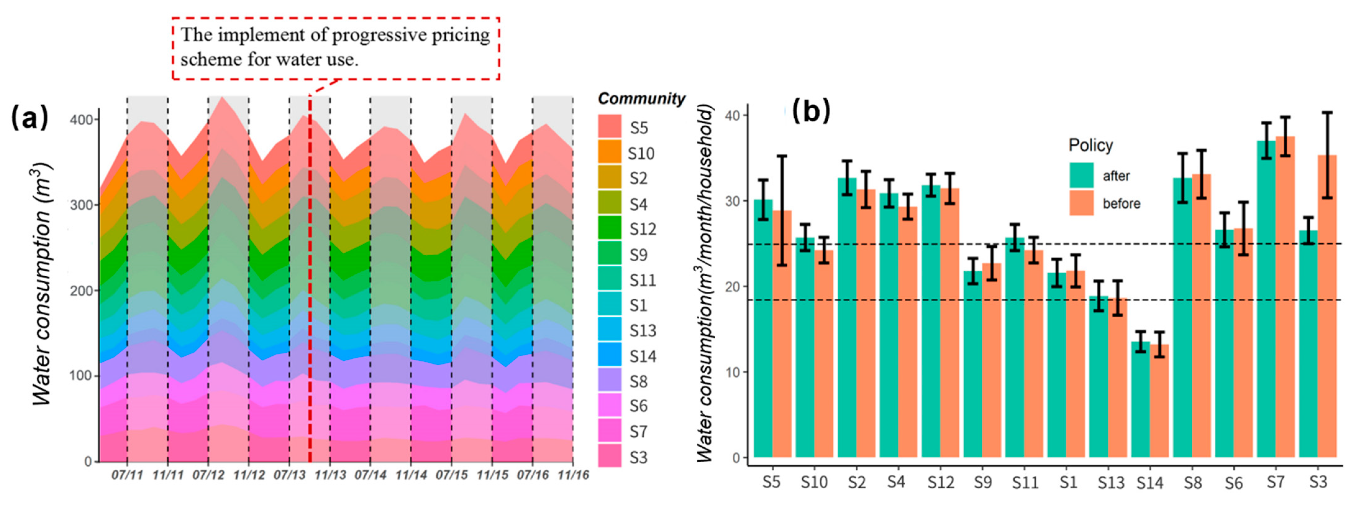
The data from Shanghai Chengtou Water Group Co., Ltd. show that the annual water use is below 220 m3 in 90.4% of the households, corresponding to 18.33 m3 per month. Accordingly, the water use in all the communities investigated was over the first progressive water price level, except for that in S14 (13.39 (±1.30) m3 per month). Figure 3a shows the variety of the water use of each household in the 14 communities across 36 months. The water use in most communities exhibited significant seasonal features for the significant difference between July and March (p = 0.0118). Communities in which there was a large fluctuation in water use are at the top of the graph. The water use of S3 and S5 shows the most significant and weakest seasonal features, respectively. The peak value of water use is found usually between August and September due to the high demand for showers, washing and irrigation in the summer. Conversely, the lowest values of water use are seen in January and February. The thicknesses of the areas indicate the values of water use. According to [32], outdoor air temperature is the most significant factor for water consumption. As shown in Figure 3a, the water use of the communities in the bottom part of the figure is usually large with weak seasonal features. There were no significant differences between water use in summer and winter in communities such as S3 (p = 0.2585) and S7 (p = 0.154), which might lead to a large degree of water use in those communities. Figure 3b shows the household water use before and after implementation of the PPS; the three levels of the PPS implemented in Shanghai are marked with dotted lines in the figure. It can be concluded that there were no significant decreases in household water use in all the communities apart from S3. The household water consumption before and after the implementation of the PPS in S3 was 35.68 (±4.97) m3 per month and 26.71 (±1.70) m3 per month, respectively. It may be because the S3 community used a lot of water before the implementation of the PPS; in addition, the houses here are older, and there are more permanent elderly residents. As can be seen, the implementation of the PPS has a great impact on S3’s water consumption. The time-series changes in the monthly average water consumption are relatively stable (Figure S3). The average water consumption of 6661 households before and after the implementation of the PPS is compared in Figure S4; it can be observed that the impact of the implementation of the PPS on residential water consumption is not significant. In other words, the use of the PPS for saving water did not reach the expected aims.
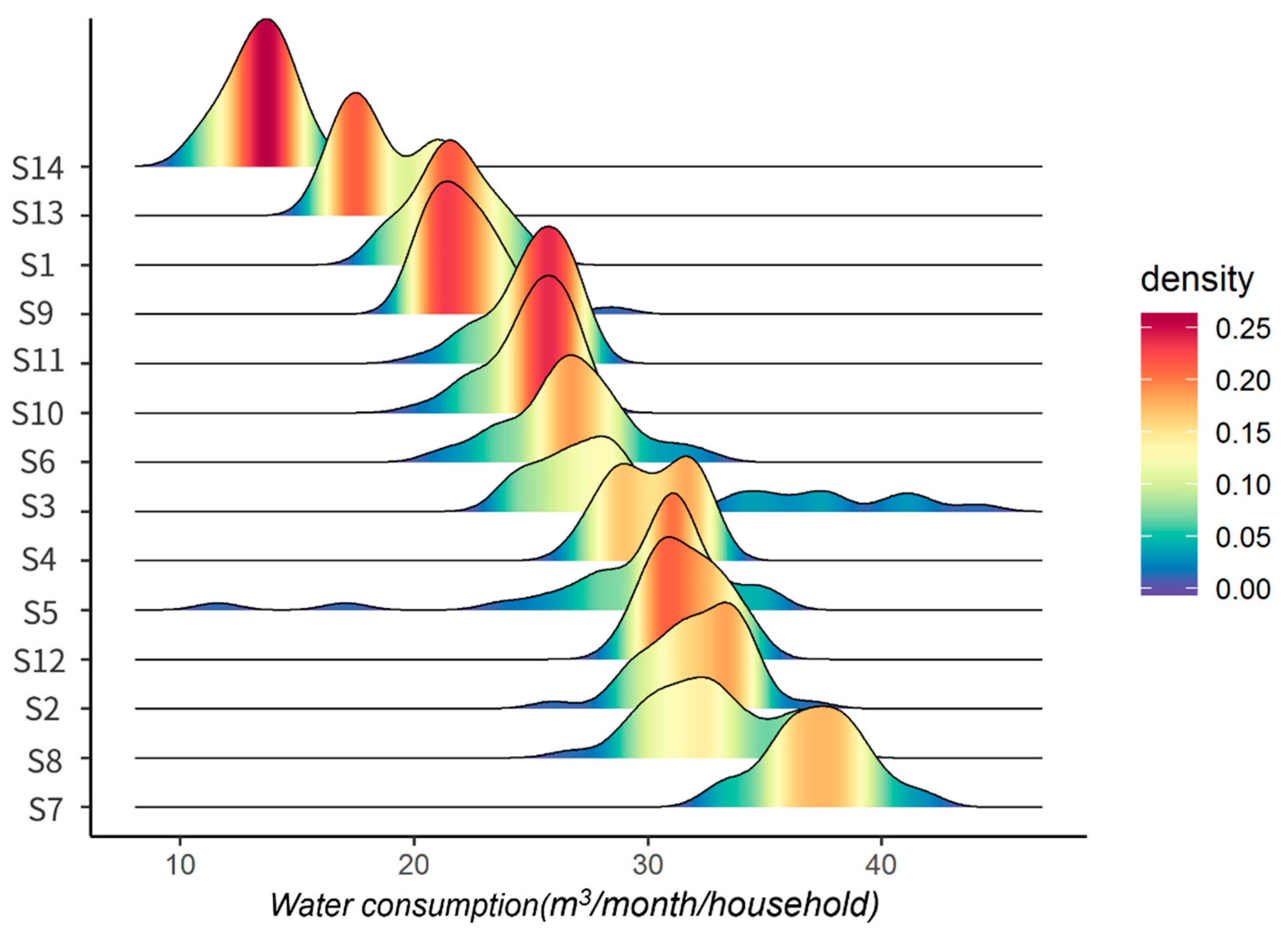
Figure 4 shows the water use of the 14 communities from 2011 to 2017. S14 had the lowest mean water use, at 13.39 (±1.30) m3, whereas S7 had the highest mean water use, at 37.25 (±2.14) m3. It is worth noting that there were large fluctuations in water consumption in communities with high water consumption, but this cannot be explained well by the seasonal effect. For instance, combined with the results of Figure 3a, the water use in S10 showed a significant seasonal variety with a concentrated density distribution, whereas that in S3 showed a weak seasonal feature with a scattered distribution. Conversely, the water use densities of the communities below S10 were concentrated and conformed relatively to the normal distribution. Water consumption was recorded on a per household basis, and the number of households had a certain impact on water consumption. Therefore, a concentrated distribution of water use might suggest a large number of permanent residents in this community and a low frequency of population mobility. In addition, the level of water consumption was relatively low in the upscale communities of S9 and S10 and the old communities of S13 and S14. As mentioned, the PPS was implemented in consideration of the economic status of the residents and their ability to pay, and they are charged in a stepped way according to the actual water consumption of the residents. However, the aim of the PPS to achieve a reasonable distribution of water resources and save water by balancing the consumption between poor and rich households has not been achieved.
3.2. Results of the PCA
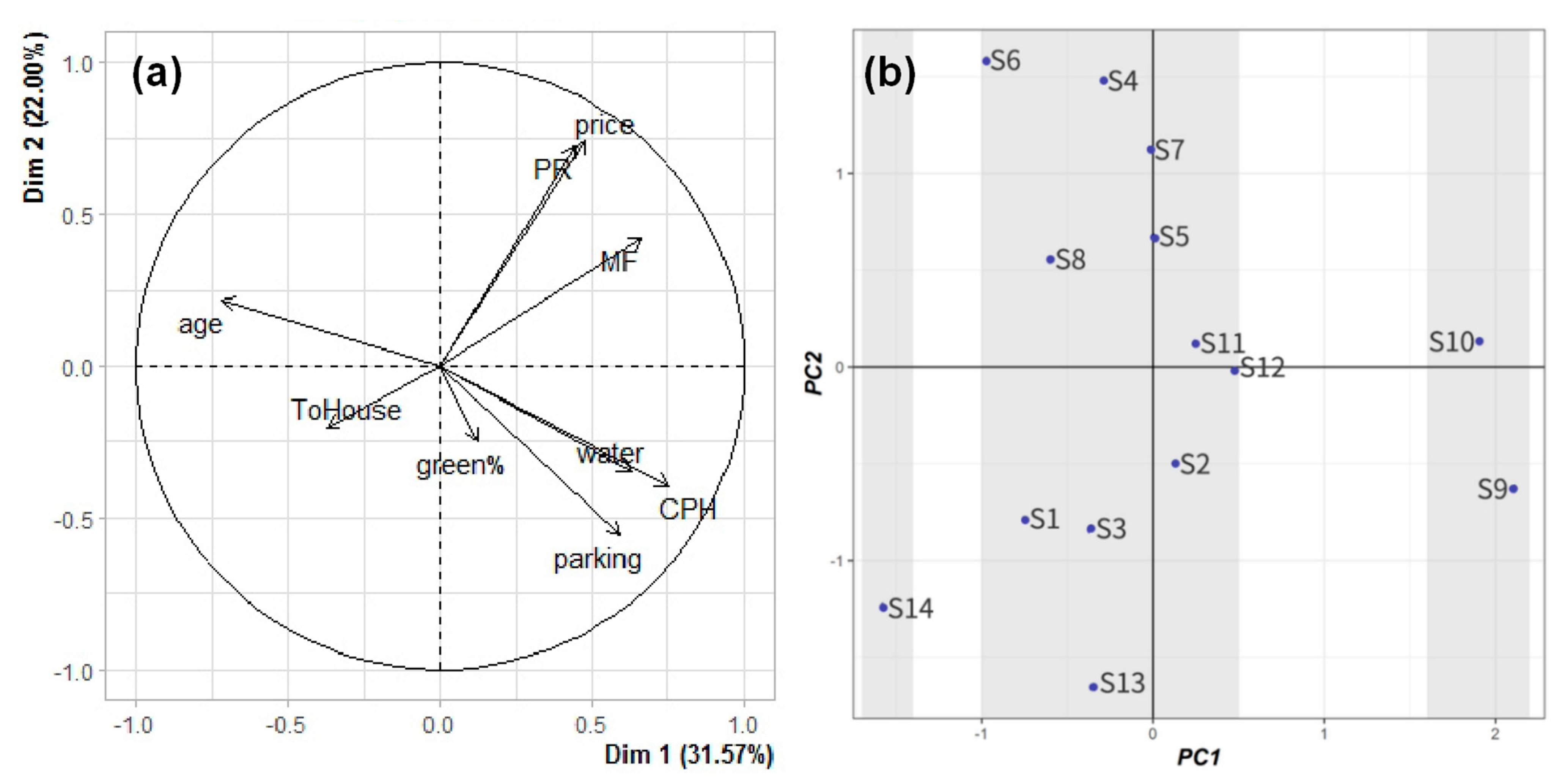
To determine the factors affecting the household water use in the 14 communities, a PCA was applied to the data matrix. The number of PCs was determined as being two, according to the results of a scree plot (Figure S5). The loadings of vectors over 0.5 were considered effective [33]. The variables green% and ToHouse were eliminated due to their low loadings on both PC1 and PC2. PC1 accounted for a total variability of 31.6% (Figure 5a). Age (−0.71), MF (0.66), parking (0.59), and CPH (0.75) had strong loadings in PC1. The communities with high prices were located in downtown districts, where management fees (MF) are usually high, corresponding to the high rental charges. An increase in the age of the community causes a decrease in water use, as the water consumers in older communities are mainly old people, and the water supply facilities of those communities have been damaged due to their long use, which affects the water supply effect. CPH and parking had positive relationships with water use. The findings indicate that communities with a higher comfort level of parking had a higher level of water consumption and a comfortable environment regarding personal car washing. The water use for car washing is usually 50 L per time [34], which accounts for a large percentage of water use in a household. Thus, PC1 contains the information of community property and can be described as the “community property component”. Both price (0.74) and PR (0.73) have strong loadings in PC2. The communities with high prices are located in downtown districts and have good location conditions. PR has a direct relationship with the comfort of the living environment. Because of the high housing prices and comfortable living conditions, the rent here is relatively high. For office workers with renting needs, this is obviously not the preferred location for renting. The low-priced community is far from the urban area, and the living environment is poor; in other words, it is not a preferred location for young people to rent. Therefore, PC2 contains the location information considered by the tenant, which can be described as the “location component”. The vector of water use has large and small loadings on PC1 (0.63) and PC2 (0.34), respectively, and it has no direct relationship with the location component. The geographical location of the community and the age of the community has a strong direct relationship with water consumption. We conducted a PCA on the community characteristics and water consumption of each year (Figure S6), and the results show that the factors affecting the community’s household water use remained unchanged from 2011 to 2017.
Figure 5b shows the scores of communities on PCs. It can be seen that S9 and S10 are far from the main cluster in the direction along the PC1 axis, which can be attributed to the high prices and good location of these two communities. S14 is far from other community points in both directions along the PC1 and the PC2 axes due to its remote position, lower housing prices, and longer age of the building. The community division along the direction of PC1 is clear, and there are three significant clusters, reflected by the shadowed areas (Figure 5b). However, in the direction along the PC2 axis, the distribution of the communities is average and could not be divided significantly. This suggests that the relationship between water use and the location factor could not be reflected by the linear algorithm of the PCA. Therefore, the effect of the location factor on the water use in the 14 communities requires further study.
3.3. Relationship between Household Water Use and Location Factors
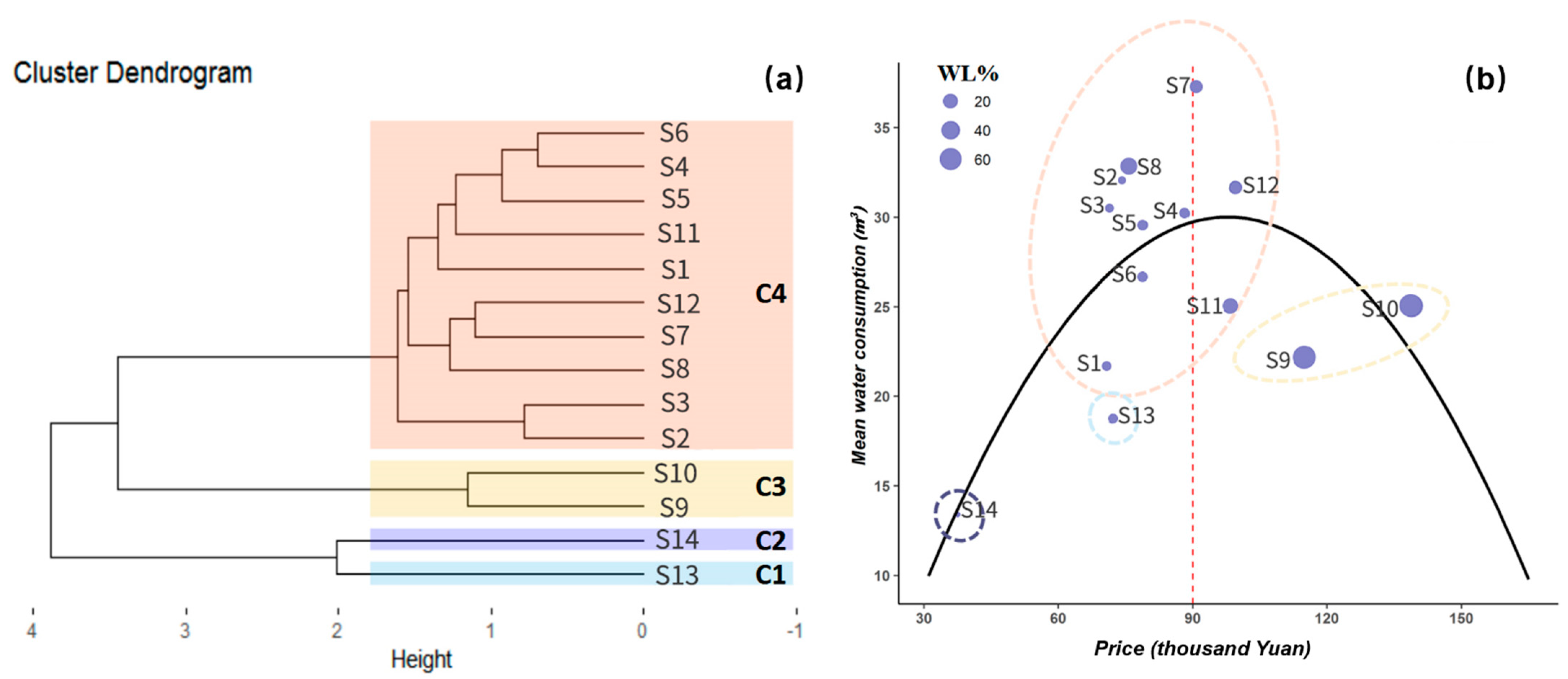
The high-end, mid-range, and low-end communities are divided according to the price and geographical location of the dwellings. At the same time, because of the higher prices, the WL of the communities is also higher (Table 1). Price and WL reflect the quality of the house. The price and WL (housing quality) in 2017 were chosen to represent the location factors. Combined with the household water use in 2017, HCA was conducted to divide the 14 communities, as shown in Figure 6a. The clusters of C1 and C2 are close due to the common low water consumption of these two communities. S9 and S10 are in the C3 cluster due to their high prices and low water use. The remaining 10 communities, which had mid-range house prices with high water use, are in the C4 cluster.
Figure 6b shows that the average water consumption of the community increases as the average house price increases up to a threshold level, after which it tends to decline as the average house price increases, showing an inverted U-shaped curve between house prices and water use. The average water consumption increased to 30 m3 until the house prices increased to CNY 90,000–100,000. With further increases in house prices, the average water consumption decreased. It is noteworthy that the inverted U-shaped curve revealed a community distribution, with WL changing. Communities S9 and S10, which had a high WL rate, used relatively less water, and a low amount of water use was observed in communities S13 and S14. S14 has been built for more than 20 years. It is far away from the urban area, housing prices are low, supporting living facilities lag behind mid-range and high-end communities, and houses are rarely rented out. Residents are mostly elderly people with a strong sense of water conservation. Therefore, S14 has low water consumption. It seems that high house prices may be related to high WL, which led to a low amount of water use. In comparison, most communities used more water as long as the house prices were relatively high. We have concluded that water consumption is related to low WL and relatively low house prices.
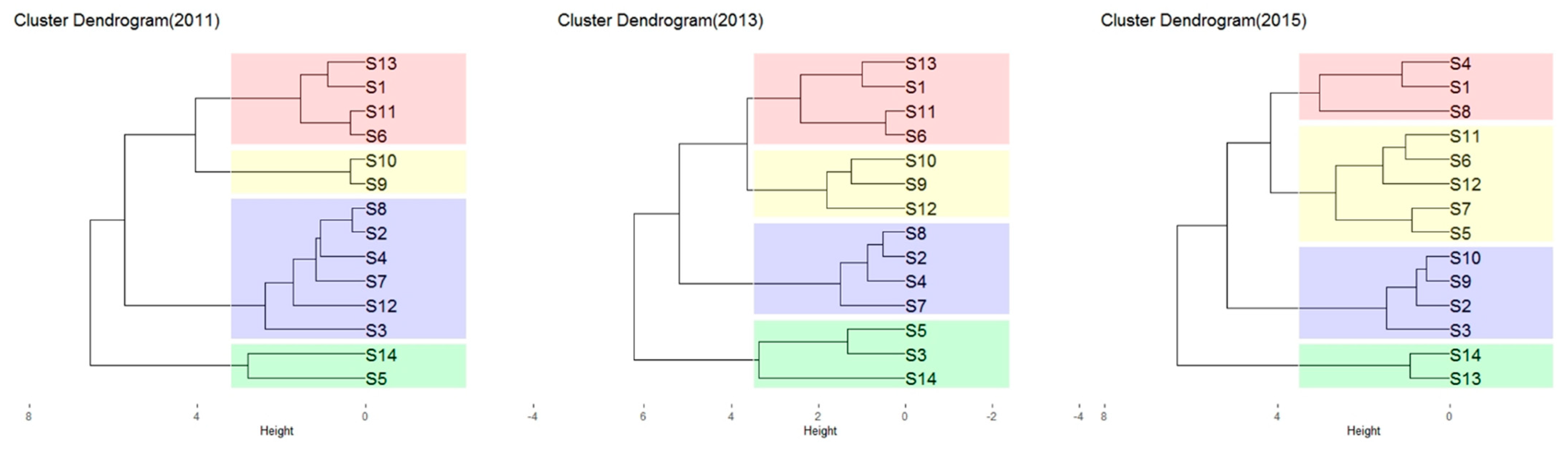
Except for housing prices, most community indexes kept near constant during 2011–2017 as the result of PCA (Figure S6). HCA analysis between water consumption and community characteristics was conducted in 2011, 2013 and 2015, compared to that of 2017. The results are shown in Figure 7. Due to the high housing prices and the good housing quality of S9 and S10, they are always in the same cluster. Before the implementation of the PPS, S13 and S14 were in distant clusters. After the implementation of the PPS, S13 and S14 are in the same cluster. This is probably relative to the low housing prices and the longer age of the houses of S13 and S14, where the elderly are the main residents. They are more sensitive to the implementation of the PPS than young generations. Although the different communities in varies years are in the same cluster, the overall change is not obvious. This is related to the housing prices and housing quality of the communities in that year. The cluster changes before and after the implementation of the PPS in 2013 are not distinct.
Before and at the beginning of the policy implementation (2011 and 2013), S13 and S14 were in distant clusters, while after the implementation of the PPS (2015 and 2017), S13 and S14 were in the same cluster and were relatively close. Changes in other communities are not obvious, they are always in the same or close clusters (2011, 2013, 2015, 2017). It shows that high-end communities (S9 and S10) are not sensitive to changes in water prices due to the high income of residents. In other communities, because of relatively low rents, there are more tenant in mid-range communities, usually in the case of several young people with independent incomes sharing a house. Their water consumption is high, but tenant did not feel that the water expenses much of an economic burden because each household has only one water meter, they split the fees between them. Water expenses will not cause them an economic burden. Therefore, the impact of the PPS on them is not obvious.
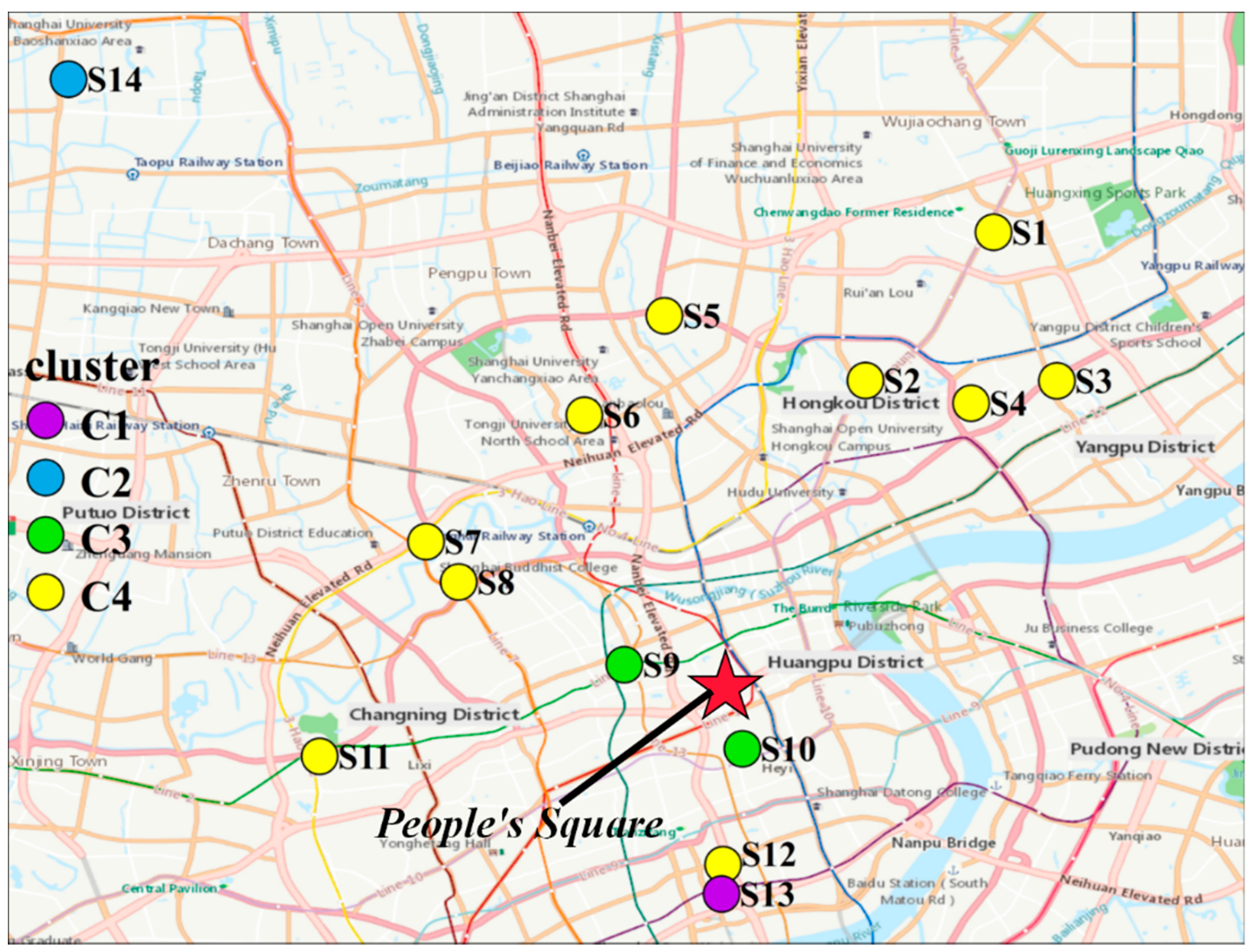
There was a significant linear relationship between price and WL (p = 0.000365). A low WL value can be explained from two points of view: (1) The percentage of rented households was large in medium-grade communities due to relatively low rental charges. (2) Due to the large number of permanent residents and the poor living conditions of old communities, there were not many houses available to be rented. In addition, rented houses in Shanghai, with water rates included, were usually paid for by several young office workers. As mentioned in the literature review, the households rented by two or more young people with independent income showed the highest water demand, conforming to that of rented households in Shanghai. Thus, in the upscale communities (S9 and S10) and old communities (S13 and S14), which had low frequencies of population mobility, most residents were permanent, leading to low and steady levels of water consumption. Older people were the main residents in old communities and there were fewer rental houses in these communities, leading to a low WL. Medium-grade communities, which were near the peak of the parabola, had a large percentage of rented households, leading to high water use. To further confirm this view, we combined the results of HCA with locations of communities, as shown in Figure 8. Taking People’s Square as the commercial center. The communities, which were far away from the commercial center (S14) and close to the commercial center (S9 and S10), had commonly low water consumption. The communities in C3, which had low WL values and high water consumption, were located around the business center of Shanghai. Thus, the findings showed that rental households were the main consumers of water.
The household water use in this study was based on the unit of community. According to the PCA results, the factors affecting the household water use in a community can be divided into two categories: the internal factor of community property and the external factor of community location. An increase in community age causes a decrease in household water use, and an increase in CPH causes an increase in household water use. Community age can reflect the age of the residents. Thus, the household water use in old communities is usually low.
3.4. Effect of the Progressive Price Scheme on Water Use
According to the results of Figure 3 and Figure 4, the PPS did not succeed in balancing the residential water resources and saving water. The response of residential water use to the PPS was not significant. The residents in the communities of the four clusters were not sensitive to the water price changes.
Most residents in the C1 and C2 communities were older people. The annual household water use of these communities was usually below 220 m3, which is necessary for daily life. The income of residents also increases year by year. This means that after the implementation of the PPS, household water expenditure as a percentage of per capita income did not change (Figure S7). Thus, the PPS did not have a significant effect on water saving in the C1 and C2 communities.
As for the communities in C4, rental units accounted for a large percentage of the total households, suggesting that occurrences of several young people sharing one dwelling unit were common in these communities. Therefore, the mean water consumption in such communities was usually high, leading to a high water price. S7 had the highest mean water use, at 37.25 (±2.14) m3 per month (447 m3 per year), and the annual water expenditure was approximately CNY 2000. However, the high cost of water use did not restrict the household water use in medium-grade communities. Even though their annual water consumption was over 300 m3 and triggered the highest water price in the PPS, it appears that tenants did not consider the water expenses to be much of an economic burden because they split the prices between themselves [35,36]. In addition, the effect of the PPS was not significant for saving water in those households.
The residents living in the communities in C3 were relatively rich people. On the one hand, people with high incomes were not sensitive to the water price [37]. On the other hand, as mentioned in the literature review, the key point affecting household water use was the number of household members [21]. The number of members in rental units was usually higher than that in non-rental households. Additionally, Figure 4 shows that the mean household water consumption of S9 was 20 m3 per month (244 m3 per year), and the annual water expenditure was approximately CNY 875. The third price grade in the PPS is likely to make residents use water comfortably [38], but the water prices were increased to promote water saving in upscale communities. However, not even rich households triggered the highest price in the PPS. Therefore, the PPS was also ineffective for the residents living in the C3 communities.
Suárez-Varela’s research found that in Spain, water costs account for only approximately 0.6% of the total household expenditure [8]. Affordability is closely related to pricing policies. Many governments and international organizations have reported water price affordability benchmarks [39]. For example, the World Bank reported 3–5%, the British government reported 3%, and the US government reported 2.5%. As New Zealand’s financial and residential statuses are similar to those of Scotland, New Zealand assumed 3% to be the benchmark for water affordability, and 57% of households in New Zealand have water fees below 3%, which seems reasonable. If the assumed value were to be higher than 3%, the low- and middle-income groups would face severe financial pressure [40]. The 2017 Shanghai Statistical Yearbook (tjj.sh.gov.cn, accessed on 1 May 2018) shows that the average annual salary of employees is CNY 85,582. Assuming that each household has only one independent income, the water fees in the 14 surveyed communities, which are CNY 550–2000, account for 0.64–2.34% of the family’s annual income. According to the “Research Report on Urban Water Shortages” by the Ministry of Urban and Rural Construction, the reasonable proportion of urban residents’ domestic water expenditure in China is 2.5–3% of the household income. A statistical survey of Shanghai residents’ water expenditures shows that per capita water expenditures account for less than 0.5% of per capita disposable income (Figure S7). Given the low proportion of water price expenditure to income, pricing schemes may not always be effective tools for modifying household water behaviors [41]. Therefore, the current water fee policy does not place an economic burden on water users.
3.5. Improvement and Promotion for PPS
As the main water consumers were rental household in medium-grade communities, with the water rate being shared by several workers, the PPS cannot effectively restrict the water use in those households. Accordingly, for those residents, the PPS needs to be adjusted in some way. At present, rental units are supported by government due to the high housing prices in Shanghai [42]. It is unreasonable to reduce rental housing. The third price grade in the PPS aims to save water use in individual households through economic pressure. However, a rental household can be regarded as a combination of several one-person households due to the economic independence of tenants. Accordingly, the water price for those rental households should be increased further to restrict the water use in the C3 communities and to cultivate their consciousness in conserving water. Research by Park and Lee [43] showed that nonprice water policies could be implemented in combination with the pricing policy in cases where the water pricing policy does not effectively reduce water demand. According to the current PPS policy, water charges account for only 0.64–2.34%, or even lower, of the total household income, and it can be assumed that they will not place a financial burden on families. Therefore, it is necessary to increase the proportion of water fee expenditure in the total household income, and use 3% as the benchmark for water affordability. According to data from the National Bureau of Statistics (http://www.stats.gov.cn/, accessed on 28 February 2018), among residents’ income and consumption expenditures in 2017, per capita residential consumption expenditures accounted for approximately one-quarter of per capita consumption expenditures. It is reasonable to use 3% as the benchmark for water affordability. At the same time, it is necessary to carry out education for the general public and publicity activities on water conservation and also to promote water-saving technologies to improve residents’ awareness of water-saving [44]. For old communities, such as S14, the water consumption of residents is low, and this will not affect the lives of residents. As for high-end communities, residents have higher incomes, and higher water charges are likely to not have a significant impact on their lives. Therefore, raising the benchmark for water affordability does not appear to place serious financial pressure on low- and middle-income groups and in turn can increase the water-saving awareness of rental households.
4. Conclusions
In this study, the effect of the progressive price scheme (PPS) for water use on the household water use in 14 communities across 6661 households was evaluated. The PPS did not reach the expectations for saving water resources and balancing consumption. The results of the principal component analysis showed that an increase in community age causes a decrease in the mean household water consumption of communities and an increase in parking causes an increase in the mean household water consumption of communities. Housing prices and WL (housing quality) showed U-shaped relationships with household water use. The hierarchical cluster analysis divided the 14 communities into 4 clusters according to the community parameters of WL, housing price, and mean household water use. Overall, we found that the rich people in upscale communities were not the main water consumers but that the rental households in medium-grade communities were. Due to water rate being split between several young tenants with independent incomes, high water price cannot restrict the water use in rental households effectively. According to data from the National Bureau of Statistics (http://www.stats.gov.cn/, accessed on 28 February 2018), among residents’ income and consumption expenditures in 2017, per capita residential consumption expenditure accounted for about a quarter of per capita consumption expenditure. A proposal was made to increase the proportion of water fee expenditure in total household income and use 3% as the benchmark for water affordability. This benchmark is based on the current proportion of water expenditure and the policies of many countries, and it may have certain limitations. This benchmark can be implemented first in megacities with better economic conditions. If water expenses account for a high proportion of household income and affect the living standards of residents, or if it is not sufficient to restrict the residents’ reasonable water use, the benchmark needs to be adjusted according to actual operating conditions. Communities can increase water-saving publicity and raise residents’ awareness of conserving water. Our study can serve as a reference for residential water use in big cities with a high frequency of population mobility.
Supplementary Materials
The following are available online at https://www.mdpi.com/article/10.3390/w13081097/s1, Figure S1: Optimal number of clusters in HCA, Figure S2: Flow chart of research method, Figure S3: Monthly changes in residential water consumption from 2011 to 2017, Figure S4: Probability density map of residential water consumption before and after the implementation of PPS, Figure S5: Gravel map to determine the factors affect the household water use in the 14 communities, Figure S6: The PCA-Biplot 9 variable loadings from 2011 to 2017 (price: house price, age: age of the house (until 2017), PR: plot ratio, MF: management fees, ToHouse: total number of households, parking: number of parking sites, CPH: number of parking sites per household, green%: green area ratio, water: the average water consumption per household in the community), Figure S7: The ratio of water expenses to per capita income in Shanghai, Table S1: Average water consumption of the community from 2011 to 2017 (m3/month/household), Table S2: Correlation coefficient matrix of variables in principal component analysis (n = 9).
Author Contributions
Investigation, data curation, writing—original draft preparation, S.H.; writing—review and editing, J.Z.; data curation, visualization, Z.L.; supervision, L.Z.; conceptualization, methodology, project administration, X.H. All authors have read and agreed to the published version of the manuscript.
Funding
This study was partially supported by National Natural Science Foundation of China (No.51678351) and the Construction and Application of Residential Secondary Water Supply Supervision System (2017ZX07207005-03).
Institutional Review Board Statement
Not applicable.
Informed Consent Statement
Not applicable.
Data Availability Statement
No new data were created or analyzed in this study. Data sharing is not applicable to this article.
Acknowledgments
The authors would like to thank the Shanghai Chengtou Water Group Co., Ltd. for providing the data used in our analysis.
Conflicts of Interest
The authors declare no conflict of interest.
References
- Goonetilleke, A.; Vithanage, M. Water Resources Management: Innovation and Challenges in a Changing World. Water 2017, 9, 281. [Google Scholar] [CrossRef]
- Irfan, M.; Kazmi, S.J.H.; Arsalan, M.H. Sustainable Harnessing of the Surface Water Resources for Karachi: A Geographic Review. Arab. J. Geosci. 2018, 11, 24. [Google Scholar] [CrossRef]
- Chu, J.; Wang, C.; Chen, J.; Wang, H. Agent-Based Residential Water Use Behavior Simulation and Policy Implications: A Case-Study in Beijing City. Water Resour. Manag. 2009, 23, 3267–3295. [Google Scholar] [CrossRef]
- Cominola, A.; Giuliani, M.; Piga, D.; Castelletti, A.; Rizzoli, A.E. Benefits and Challenges of Using Smart Meters for Advancing Residential Water Demand Modeling and Management: A Review. Environ. Model. Softw. 2015, 72, 198–214. [Google Scholar] [CrossRef] [Green Version]
- Seelen, L.M.S.; Flaim, G.; Jennings, E.; De Senerpont Domis, L.N. Saving Water for the Future: Public Awareness of Water Usage and Water Quality. J. Environ. Manag. 2019, 242, 246–257. [Google Scholar] [CrossRef]
- Xue, P.; Hong, T.; Dong, B.; Mak, C. A Preliminary Investigation of Water Usage Behavior in Single-Family Homes. Build. Simul. 2017, 10, 949–962. [Google Scholar] [CrossRef] [Green Version]
- Rees, P.; Clark, S.; Nawaz, R. Household Forecasts for the Planning of Long-Term Domestic Water Demand: Application to London and the Thames Valley. Popul. Space Place 2020, 26. [Google Scholar] [CrossRef]
- Suárez-Varela, M. Modeling Residential Water Demand: An Approach Based on Household Demand Systems. J. Environ. Manag. 2020, 261, 109921. [Google Scholar] [CrossRef]
- Chen, X.; Li, F.; Li, X.; Hu, Y.; Hu, P. Evaluating and Mapping Water Supply and Demand for Sustainable Urban Ecosystem Management in Shenzhen, China. J. Clean. Prod. 2020, 251, 119754. [Google Scholar] [CrossRef]
- Lu, S.; Gao, X.; Li, W.; Jiang, S.; Huang, L. A Study on the Spatial and Temporal Variability of the Urban Residential Water Consumption and Its Influencing Factors in the Major Cities of China. Habitat Int. 2018, 78, 29–40. [Google Scholar] [CrossRef]
- Torres López, S.; de los Angeles Barrionuevo, M.; Rodríguez-Labajos, B. Water Accounts in Decision-Making Processes of Urban Water Management: Benefits, Limitations and Implications in a Real Implementation. Sustain. Cities Soc. 2019, 50, 101676. [Google Scholar] [CrossRef]
- Wang, H.; Xie, J.; Li, H. Water Pricing with Household Surveys: A Study of Acceptability and Willingness to Pay in Chongqing, China. China Econ. Rev. 2010, 21, 136–149. [Google Scholar] [CrossRef]
- Polebitski, A.S.; Palmer, R.N. Seasonal Residential Water Demand Forecasting for Census Tracts. J. Water Resour. Plan. Manag. 2010, 136, 27–36. [Google Scholar] [CrossRef]
- Otaki, Y.; Otaki, M.; Aramaki, T. Combined Methods for Quantifying End-Uses of Residential Indoor Water Consumption. Environ. Process. 2017, 4, 33–47. [Google Scholar] [CrossRef]
- Voskamp, I.M.; Sutton, N.B.; Stremke, S.; Rijnaarts, H.H.M. A Systematic Review of Factors Influencing Spatiotemporal Variability in Urban Water and Energy Consumption. J. Clean. Prod. 2020, 256, 120310. [Google Scholar] [CrossRef]
- Zheng, J.; Kamal, M.A. The Effect of Household Income on Residential Wastewater Output: Evidence from Urban China. Util. Policy 2020, 63, 101000. [Google Scholar] [CrossRef]
- Taştan, H. Estimation of Dynamic Water Demand Function: The Case of Istanbul. Urban Water J. 2018, 15, 75–82. [Google Scholar] [CrossRef]
- Richter, C.P.; Stamminger, R. Water Consumption in the Kitchen—A Case Study in Four European Countries. Water Resour Manag. 2012, 26, 1639–1649. [Google Scholar] [CrossRef]
- Seidl, C.; Wheeler, S.A.; Zuo, A. High Turbidity: Water Valuation and Accounting in the Murray-Darling Basin. Agric. Water Manag. 2020, 230, 105929. [Google Scholar] [CrossRef]
- Kotagama, H.; Zekri, S.; Al Harthi, R.; Boughanmi, H. Demand Function Estimate for Residential Water in Oman. Int. J. Water Resour. Dev. 2017, 33, 907–916. [Google Scholar] [CrossRef]
- Rajeevan, U.; Mishra, B.K. Sustainable Management of the Groundwater Resource of Jaffna, Sri Lanka with the Participation of Households: Insights from a Study on Household Water Consumption and Management. Groundw. Sustain. Dev. 2020, 10, 100280. [Google Scholar] [CrossRef]
- Mayol, A. Social and Nonlinear Tariffs on Drinking Water: Cui Bono? Empirical Evidence from a Natural Experiment in France. Rev. D’économie Polit. 2017, 127, 1161. [Google Scholar] [CrossRef]
- Mostafavi, N.; Shojaei, H.R.; Beheshtian, A.; Hoque, S. Residential Water Consumption Modeling in the Integrated Urban Metabolism Analysis Tool (IUMAT). Resour. Conserv. Recycl. 2018, 131, 64–74. [Google Scholar] [CrossRef]
- Makki, A.A.; Stewart, R.A.; Panuwatwanich, K.; Beal, C. Revealing the Determinants of Shower Water End Use Consumption: Enabling Better Targeted Urban Water Conservation Strategies. J. Clean. Prod. 2013, 60, 129–146. [Google Scholar] [CrossRef] [Green Version]
- Barraqué, B.O.; Laigneau, P.; Formiga-Johnsson, R.M. The Rise and Fall of the French Agences de l’Eau: From German-Type Subsidiarität to State Control. Water Econ. Policy 2018, 4, 1850013. [Google Scholar] [CrossRef]
- De Brito, P.L.C.; de Azevedo, J.P.S. Charging for Water Use in Brazil: State of the Art and Challenges. Water Resour. Manag. 2020, 34, 1213–1229. [Google Scholar] [CrossRef]
- Wang, Y.; Tian, K.; Wang, H.; Zhang, B. Regional Differences in Citizens’ Water Behaviors: A Comparative Study of Typical Cities Based on AMOS. Water Policy 2019, 21, 742–757. [Google Scholar] [CrossRef]
- Tong, Y.; Fan, L.; Niu, H. Water Conservation Awareness and Practices in Households Receiving Improved Water Supply: A Gender-Based Analysis. J. Clean. Prod. 2017, 141, 947–955. [Google Scholar] [CrossRef]
- Wang, C.-H.; Dong, H. Responding to the Drought: A Spatial Statistical Approach to Investigating Residential Water Consumption in Fresno, California. Sustainability 2017, 9, 240. [Google Scholar] [CrossRef] [Green Version]
- Kazor, K.; Holloway, R.W.; Cath, T.Y.; Hering, A.S. Comparison of Linear and Nonlinear Dimension Reduction Techniques for Automated Process Monitoring of a Decentralized Wastewater Treatment Facility. Stoch Environ. Res. Risk Assess. 2016, 30, 1527–1544. [Google Scholar] [CrossRef]
- Snelder, T.H.; Booker, D.J. Natural flow regime classifications are sensitive to definition procedures. River Res. Appl. 2013, 29, 822–838. [Google Scholar] [CrossRef]
- Zheng, H.; Zhou, W.; Zhang, L.; Li, X.; Cheng, J.; Ding, Z.; Xu, Y.; Hu, W. Urban Water Consumption Patterns in an Adult Population in Wuxi, China: A Regression Tree Analysis. IJERPH 2020, 17, 2983. [Google Scholar] [CrossRef] [PubMed]
- Tamura, M.; Tsujita, S. A Study on the Number of Principal Components and Sensitivity of Fault Detection Using PCA. Comput. Chem. Eng. 2007, 31, 1035–1046. [Google Scholar] [CrossRef]
- Villarreal, E.L.; Dixon, A. Analysis of a Rainwater Collection System for Domestic Water Supply in Ringdansen, Norrköping, Sweden. Build. Environ. 2005, 40, 1174–1184. [Google Scholar] [CrossRef]
- Jessoe, K.; Papineau, M.; Rapson, D. Utilities Included: Split Incentives in Commercial Electricity Contracts. Energy J. 2020, 41. [Google Scholar] [CrossRef] [Green Version]
- Melvin, J. The Split Incentives Energy Efficiency Problem: Evidence of Underinvestment by Landlords. Energy Policy 2018, 115, 342–352. [Google Scholar] [CrossRef]
- Wichman, C.J.; Taylor, L.O.; von Haefen, R.H. Conservation Policies: Who Responds to Price and Who Responds to Prescription? J. Environ. Econ. Manag. 2016, 79, 114–134. [Google Scholar] [CrossRef] [Green Version]
- Mayol, A.; Porcher, S. Tarifs discriminants et monopoles de l’eau potable: Une analyse de la réaction des consommateurs face aux distorsions du signal-prix. Rev. Économique 2019, 70, 461. [Google Scholar] [CrossRef]
- Tortajada, C.; González-Gómez, F.; Biswas, A.K.; Buurman, J. Water Demand Management Strategies for Water-Scarce Cities: The Case of Spain. Sustain. Cities Soc. 2019, 45, 649–656. [Google Scholar] [CrossRef]
- Mahmood, B.; Sharma, S. Affordability of Household Water and Wastewater Charges in Manukau City: A Case Study. In WIT Transactions on Ecology and the Environment; WIT Press: Boston, MA, USA, 2009; pp. 313–324. [Google Scholar]
- Reynaud, A.; Romano, G. Advances in the Economic Analysis of Residential Water Use: An Introduction. Water 2018, 10, 1162. [Google Scholar] [CrossRef] [Green Version]
- Chen, J.; Hao, Q.; Stephens, M. Assessing Housing Affordability in Post-Reform China: A Case Study of Shanghai. Hous. Stud. 2010, 25, 877–901. [Google Scholar] [CrossRef]
- Park, H.; Lee, D.K. Is Water Pricing Policy Adequate to Reduce Water Demand for Drought Mitigation in Korea? Water 2019, 11, 1256. [Google Scholar] [CrossRef] [Green Version]
- Grafton, R.Q.; Ward, M.B.; To, H.; Kompas, T. Determinants of Residential Water Consumption: Evidence and Analysis from a 10-Country Household Survey: Determinants of Residential Water Consumption. Water Resour. Res. 2011, 47. [Google Scholar] [CrossRef] [Green Version]
Figure 1.
Spatial distribution of the 14 investigated communities in Shanghai.

Figure 2.
The relationship between WL (%) and water consumption (WL: the ratio of unoccupied houses on the rental market to the total number of households).
Figure 2.
The relationship between WL (%) and water consumption (WL: the ratio of unoccupied houses on the rental market to the total number of households).

Figure 3.
(a) Area plot (month/year) of the water use per household in the 14 communities. Grey areas refer to summer periods. Area’s height means the quantity of water use. (b) The household water consumption (m3) before and after the implement of progressive pricing scheme for water use.
Figure 3.
(a) Area plot (month/year) of the water use per household in the 14 communities. Grey areas refer to summer periods. Area’s height means the quantity of water use. (b) The household water consumption (m3) before and after the implement of progressive pricing scheme for water use.

Figure 4.
The density curves of water use per household (m3) during 2011–2017 in the 14 communities.
Figure 4.
The density curves of water use per household (m3) during 2011–2017 in the 14 communities.

Figure 5.
(a) The plot of 9 variable loadings with varimax rotation. (b) The plot of principal component scores of the 14 communities on PCs: price, housing price; age, age of the building (until 2017); PR, plot ratio; MF, management fees; ToHouse, total number of households; parking, number of parking sites; CPH, number of parking sites per household; green%, green area ratio; water, the average water consumption per household in the community.

Figure 6.
(a) The dendrogram of the 14 communities through hierarchical cluster analysis. (b) The relationship between price and mean water consumption of the 14 communities. Red line means the average price of the house in the center areas of Shanghai. The significance level of t-test is accepted as the p value was less than 0.05. (price: house price, WL: the ratio of unoccupied houses on the rental market to the total number of households).

Figure 7.
The dendrogram of the 14 communities through hierarchical cluster analysis (2011, 2013, 2015).
Figure 7.
The dendrogram of the 14 communities through hierarchical cluster analysis (2011, 2013, 2015).

Figure 8.
The spatial distribution of the 14 communities with their cluster characteristics.


Table 1.
Abbreviations and descriptions of 10 variables.
| Name | Abbreviation | Description |
|---|---|---|
| Housing price | price | Housing prices can reflect the consumption power of residents. |
| Age of the building (until 2017) | age | The newness of the community indirectly represents the level of living facilities in the community. |
| Plot ratio | PR | Plot ratio refers to the ratio of the total building area above the ground to the area of land available for construction. The floor area ratio directly relates to the comfort of living. The smaller the plot ratio is, the better the community environment is considered to be. |
| Management fees | MF | The high management fee indicates that the overall environment of the community is good. |
| Total number of households | ToHouse | The number of houses in the community is large, and the population is also relatively large; large communities with large populations can often receive attention from the government. |
| Number of parking sites | parking | The number of parking sites is one of the criteria for measuring the quality of the community. |
| Number of parking sites per household | CPH | CPH is a measure of the parking space for one household, reflecting the comfort level of parking. |
| Greening area ratio | green% | The higher the greening rate and the lower the building density, the more comfortable the residents. |
| Ratio of unoccupied houses on the rental market to the total number of households | WL | The ratio indicates the houses waiting to be rented; WL is calculated based on the ratio of the number of residents whose water consumption is 0 m3 in the monthly water bill to the total number of households in the community. When WL is high, the number of houses waiting to be rented out is large, and the number of residents in the community is relatively small. |
| Average water consumption per household in the community | water | The total community consumption is divided by the number of houses occupied in the community. |
Table 2.
The parameters of the 14 investigated communities in 2017.
| Community | Prices (10 Thousand CNY/m2) | Age (year) | PR | MF (CNY/m2) | Parking (per) | ToHouse (households) | CPH | WL (%) | Green (%) | Water (m3/month/household) |
|---|---|---|---|---|---|---|---|---|---|---|
| S1 | 7.1 | 10 | 2.3 | 1.5 | 150 | 1540 | 0.10 | 6.43 | 30 | 20.73 |
| S2 | 7.4 | 14 | 3.5 | 1 | 100 | 239 | 0.42 | 4.18 | 38 | 29.31 |
| S3 | 7.1 | 18 | 1.8 | 2.7 | 120 | 659 | 0.18 | 6.07 | 41 | 25.44 |
| S4 | 8.8 | 11 | 2.9 | 2.5 | 807 | 670 | 1.20 | 9.70 | 20 | 32.20 |
| S5 | 7.9 | 7 | 2.6 | 2.3 | 527 | 776 | 0.68 | 8.25 | 50 | 28.29 |
| S6 | 7.9 | 12 | 2.5 | 1.8 | 1200 | 1126 | 1.07 | 9.59 | 35 | 25.66 |
| S7 | 9.1 | 10 | 2.5 | 4 | 700 | 993 | 0.70 | 14.20 | 46 | 33.55 |
| S8 | 7.6 | 9 | 2.1 | 1 | 500 | 1160 | 0.43 | 29.31 | 42 | 33.08 |
| S9 | 11.5 | 10 | 3.5 | 5 | 248 | 452 | 0.55 | 72.35 | 29 | 20.32 |
| S10 | 13.9 | 11 | 4.0 | 3 | 500 | 708 | 0.71 | 66.81 | 45 | 26.25 |
| S11 | 9.8 | 9 | 4.6 | 4 | 496 | 1465 | 0.34 | 23.89 | 30 | 26.25 |
| S12 | 9.9 | 13 | 3.8 | 2.5 | 400 | 1053 | 0.38 | 16.90 | 40 | 30.47 |
| S13 | 7.2 | 27 | 3.4 | 1.35 | 200 | 1151 | 0.17 | 6.43 | 32 | 18.02 |
| S14 | 3.8 | 21 | 1.7 | 0.45 | 300 | 1156 | 0.26 | 2.00 | 35 | 13.82 |
Publisher’s Note: MDPI stays neutral with regard to jurisdictional claims in published maps and institutional affiliations. |
© 2021 by the authors. Licensee MDPI, Basel, Switzerland. This article is an open access article distributed under the terms and conditions of the Creative Commons Attribution (CC BY) license (https://creativecommons.org/licenses/by/4.0/).
Share and Cite
MDPI and ACS Style
Han, S.; Zhou, J.; Liu, Z.; Zhang, L.; Huang, X. Influence of Community Factors on Water Saving in a Mega City after Implementing the Progressive Price Schemes. Water 2021, 13, 1097. https://doi.org/10.3390/w13081097
AMA Style
Han S, Zhou J, Liu Z, Zhang L, Huang X. Influence of Community Factors on Water Saving in a Mega City after Implementing the Progressive Price Schemes. Water. 2021; 13(8):1097. https://doi.org/10.3390/w13081097
Chicago/Turabian StyleHan, Shaohong, Jizhi Zhou, Zeyuan Liu, Lijian Zhang, and Xin Huang. 2021. "Influence of Community Factors on Water Saving in a Mega City after Implementing the Progressive Price Schemes" Water 13, no. 8: 1097. https://doi.org/10.3390/w13081097
Note that from the first issue of 2016, this journal uses article numbers instead of page numbers. See further details here.