
The Performance of Physically Based and Conceptual Hydrologic Models: A Case Study for Makkah Watershed, Saudi Arabia


1
Department of Civil and Environmental Engineering, King Fahd University of Petroleum and Minerals (KFUPM), Dhahran 31261, Saudi Arabia
2
Department of Civil and Environmental Engineering, University of Texas at San Antonio, San Antonio, TX 78249, USA
*
Author to whom correspondence should be addressed.
Water 2021, 13(8), 1098; https://doi.org/10.3390/w13081098
Submission received: 26 February 2021
/
Revised: 12 April 2021
/
Accepted: 13 April 2021
/
Published: 16 April 2021
Abstract
:Population growth and land use modification in urban areas require the use of accurate tools for rainfall-runoff modeling, especially where the topography is complex. The recent improvement in the quality and resolution of remotely sensed precipitation satisfies a major need for such tools. A physically-based, fully distributed hydrologic model and a conceptual semi-distributed model, forced by satellite rainfall estimates, were used to simulate flooding events in a very arid, rapidly urbanizing watershed in Saudi Arabia. Observed peak discharge for two flood events was used to compare hydrographs simulated by the two models, one for calibration and one for validation. To further explore the effect of watershed heterogeneity, the hydrographs produced by three implementations of the conceptual were compared against each other and against the output of the physically-based model. The results showed the ability of the distributed models to capture the effect of the complex topography and variability of land use and soils of the watershed. In general, the GSSHA model required less calibration and performed better than HEC-HMS. This study confirms that the semi-distributed HEC-HMS model cannot be used without calibration, while the GSSHA model can be the best option in the case of a lack of data. Although the two models showed good agreement at the calibration point, there were significant differences in the runoff, discharge, and infiltration values at interior points of the watershed.
1. Introduction
Hydrologic models are used to solve a range of specific problems in the management and development of water and land resources, including flood simulation and prediction, aquifer recharge management, runoff estimation, and drainage network design (e.g., [1,2,3]). The uncertainties inherent in these models can be reduced with the availability of accurate input and watershed data [4]. Hydrologic models include lumped models, semi-distributed models, or fully distributed models [5]. These models can also be classified based on the model formulation as empirical or physically-based models with conceptual formulations typically used in lumped models and physical equations in the other two types [6]. The parameters of the lumped models are not directly related to the watershed’s physical characteristics, which is an important shortcoming of these models [7]. Generally, the application of lumped models is limited to gauged watersheds not undergoing significant change in their conditions, and they have to be calibrated using significant observational data [7].
In a semi-distributed model, the basin to be simulated is divided into smaller sub-basins to capture the spatial variability of the inputs and to represent the heterogeneity within the basin [8]. The data required for a semi-distributed model is typically less than that needed for a fully distributed model. In addition, the spatial representation and mathematical formulations of the hydrologic processes are simpler [9]. Although a semi-distributed model requires a limited number of parameters compared to a fully distributed model, it requires more calibration data [10]. In general, the natural spatial and temporal variations of the hydrological properties such as soil type, land use, and rainfall are not accurately represented in the semi-distributed hydrologic models [11].
The fully distributed models try to simulate the watershed conditions accurately while the physical processes and/or the spatial heterogeneity are mathematically treated at the grid cell scale [12,13]. The distributed models can be either empirically distributed models or physically-based distributed models. The difference between them is the transformation of the surface runoff, which is empirically simulated in empirical distributed models and through physical formulations in physically-based distributed models [14]. The model grid size is selected based on the required level of detail of runoff simulations and the spatial resolution of inputs and watershed data [15,16].
Several studies have compared different types of hydrologic models. Paudel et al. [17] compared the performances of lumped and distributed models and concluded that the simulation of land use changes using distributed models is significantly better than using lumped models. Sith & Nadaoka [18] found that the physically-based, fully distributes model GSSHA (Gridded Surface/Subsurface Hydrologic Analysis) performed slightly better than the semi-distributed, semi-physically-based model SWAT (the Soil and Water Assessment Tool) for short-term streamflow simulations, while, for long-term simulations, both models had acceptable performance. Hui-lan [19] concluded that the hydrographs predicted by a distributed model compared with field observations were much better than those predicted by a semi-distributed model. El-Nasr et al. [20] found that the semi-distributed SWAT model and the fully distributed MIKE SHE model performed well when used to simulate the hydrology of a large catchment, but the MIKE SHE model was slightly better. Meselhe et al. [21] investigated the impact of spatial and temporal sampling of rainfall on runoff predictions using a conceptual and physically-based hydrologic model over a small watershed. They found that the physically-based hydrologic model was more sensitive to both the temporal and spatial samplings of rainfall than the conceptual model. Other researchers evaluated the performance of HEC-HMS (the Hydrologic Engineering Center-Hydrologic Modelling System) and GSSHA models and reported a much better performance by GSSHA (e.g., [22,23]).
Several hydrologic studies have been conducted in the Arab Peninsula using different modeling approaches. Al Abdouli et al. [24] used HEC-HMS to quantify coastal runoff and examine its temporal and spatial distribution in several watersheds in the United Arab Emirates (UAE) to assess the potential for recharge of depleted aquifers and flood mitigation in urban areas. Sharif et al. [25] simulated an extreme flood event in Hafr Al Batin city, Saudi Arabia using the physically-based, fully-Distributed Hydrologic model (GSSHA) driven by Global Precipitation Measurement (GPM) satellite rainfall data. Their results demonstrated that the urban portion, which is 6.8% of the watershed area, produced about 85% of the generated runoff. Embaby et al. [26] developed an integrated approach combining geotechnical investigation and hydrologic modeling to generate hazard zones for Tabuk city, Saudi Arabia. The approach was successful in identifying areas prone to flooding. Al-Zahrani et al. [6] developed a flood hazard map for Hafr Al-Batin city by integrating the results of three models (hydrologic, hydraulic, and flood delineation models). They recommended that their result can be used for designing flood control structures and other planning purposes. Fathy et al. [27] evaluated hydrologic models over Wadi Sudr, Sinia, Egypt, and found that the runoff hydrograph can be estimated more accurately using the distributed model. To the authors’ knowledge, no study tried to investigate the differences between conceptual semi-distributed and physically-based fully distributed models in simulating extreme flood events in the region.
In recent years, the Makkah region in western Saudi Arabia has been suffering from an increase in the frequency of flash floods due to its natural complex topography, which is dominated by mountains with steep slopes and very shallow soil layers. These events are triggered by the occurrence of infrequent high convective short-lived rainfall events. A few hydrologic studies have been performed in the Makkah region. However, all studies used lumped or semi-distributed models and were mostly focused on simulating peak discharge. Abdelkarim & Gaber [28] assessed the impact of flash flooding in the Makkah area by constructing a flood risk map for a watershed in Makkah City using HEC-HMS and HEC-RAS. Their findings suggested a flood control policy based on using the existing hydraulic facilities and a range of new structures that can help protect lives and the urban infrastructure. Elfeki et al. [29] evaluated the flood hazard on another watershed in Makkah, also using HEC-HMS and HEC-RAS, and recommended some structural measures to mitigate floods. Bastawesy et al. [30] assessed the potential of flash flooding in a third watershed in Makkah using GIS and recommended a range of mitigation measures to contain the 50-year design flood. Dawod et al. [31] applied simple hydrologic models and four national regression models to estimate the flood peak discharge in several ungauged small watersheds in Makkah. They concluded that the Curve Number (CN) approach is the best methodology for flood estimation in case of the availability of soil type, land use, and metrological data. Al-ghamdi et al. [32] used the Curve Number method to estimate flood hazards in Makkah City for the period 1990 and 2010. They found that the expansion of the residential areas was behind the significant rise in significant flood hazards. Al Saud [33] analyzed the morphometry of Wadi Aurnah, Makkah, using GIS and introduced a simple approach for rapid assessment of the flooding potential.
The main goal of this study is to simulate recent floods in the Makkah region using a physically-based fully distributed hydrologic model and compare its performance to that of the semi-distributed HEC-HMS model. Two flood events that occurred in 2010 and 2018 were used in this study. One event was used for model calibration and the other for validation. The difference in model output was discussed and was further investigated by comparing the different implementations of HEC-HMS to explore the impact of watershed heterogeneity on the model results.
2. Study Area
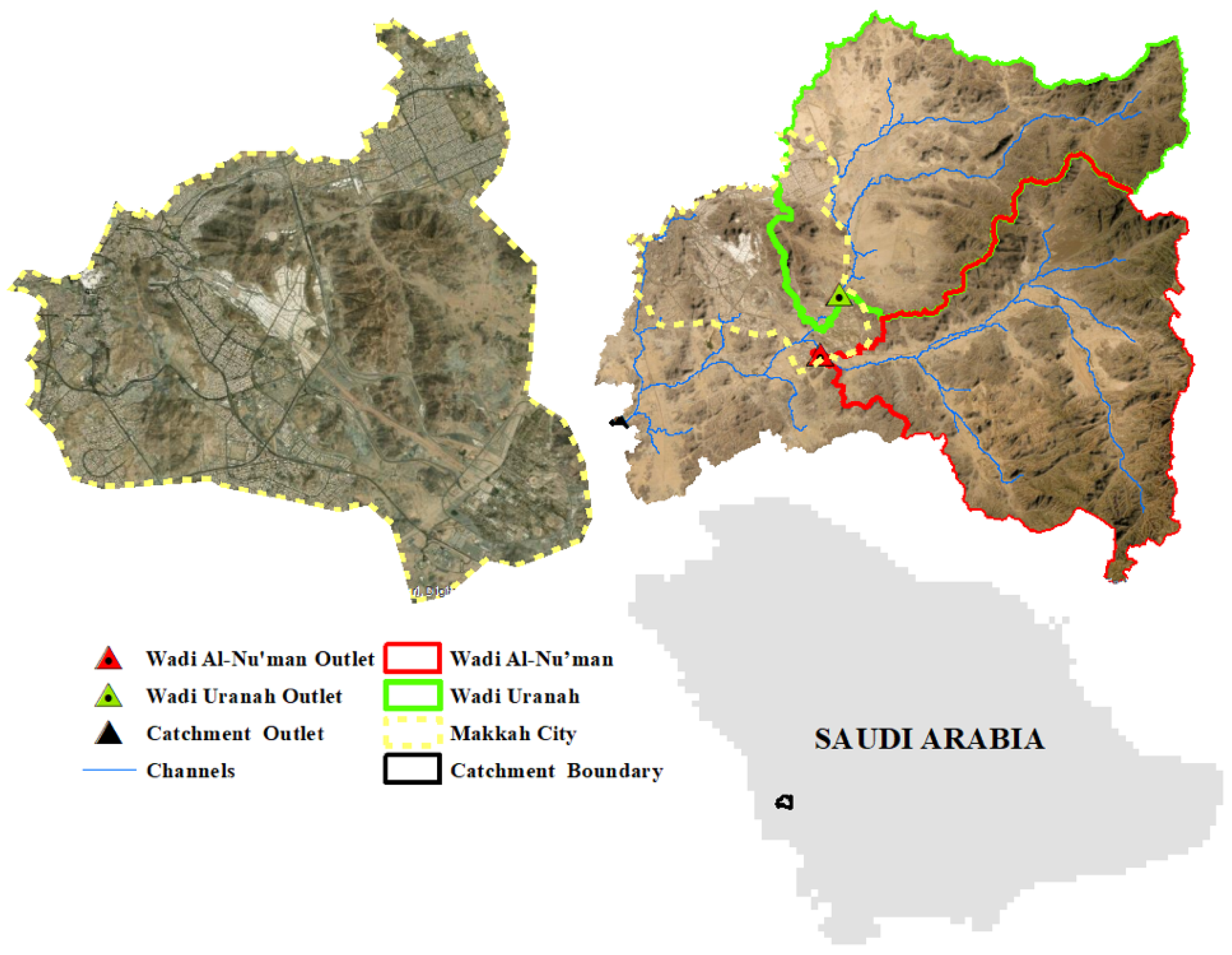
Makkah province is one of thirteen provinces in Saudi Arabia and is considered one of the most important regions due to its location in the historic Hejaz region and its extended coastline on the Red Sea. The total area of Makkah region is approximately 153,200 km2 occupied by around 8,557,000 people [34], making it the third-largest and most populous province. The city of Makkah (Makkah Al-Mukarramah), the Makkah Province’s capital, is located 70 km from Jeddah on the Red Sea with an average elevation of 277 m above sea level. The region is characterized by a dry climate with sparse, inconsistent rainfall events [35]. Plains and mountains are the main geomorphological units of the study area. In the past few decades, the city of Makkah has witnessed unusually rapid urbanization, making it the third most populated metropolitan area in Saudi Arabia. The increase in the urban areas in Makkah province between 1992 and 2013 was threefold, as reported by Alahmadi & Atkinson [36]. This growth is mainly due to the significant increase in the area covered by Makkah City from about 12% of the province in 1992 to 22% in 2016 [37]. Recently, Abdelkarim & Gaber [28] reported that the urban areas exposed to flooding have increased by approximately 25 fold between 1988 and 2019. In addition, a high percentage of Makkah’s road network (more than 50%) is subjected to inundation during major flood events [36]. Because of the rapid urban growth, municipal authorities now require flood impact studies being conducted before any land development activity within the city limits. The Makkah watershed used in this study was delineated using a high-resolution digital elevation model (DEM) of 10 m obtained from King Abdulaziz City of Science and Technology (KACST). The delineated watershed includes most of Makkah city with a drainage area of 1725 km2 (Figure 1).
3. Rainfall Events
The calibration and validation run of the two models were driven by two storm events that occurred recently in the Makkah watershed. Due to the very sparse rain gauge network in the study area, capturing the features of the extreme precipitation through ground observations was not possible. Moreover, the very limited rain gauge data are available only at a daily time scale. Therefore, the two hydrologic models were forced using the satellite rainfall data, which would have the ability to capture the spatial and temporal variability of the storm events at much higher resolutions.
A previous study by the authors using the Integrated Multi-satellitE Retrievals for GPM (IMERG) satellite rainfall products showed reasonable performance of the IMERG Early run product in the Makkah region compared to the other IMERG products. Accordingly, the two simulated models were forced by the IMERG Early run product in this study. The IMERG Early run data with spatial and temporal resolutions of 0.1° × 0.1° and 30 min were downloaded using FileZilla software from the Precipitation Measurement Missions (PMM) website (http://pmm.nasa.gov/data-access/downloads/gpm (accessed on 7 March 2020)). The data were converted from HDF5 into a gridded ASCII format using an R script developed by the authors and was then reformatted as input to the hydrologic model. The latest version of the IMERG product, Version 6 (IMERG-V06), was used. The latest product includes significant updates such as a higher maximum rainfall threshold from 50 to 200 mm/h, full inter-calibration to the GPM combined instrument dataset, and the use of an updated rain retrieval algorithm [38].
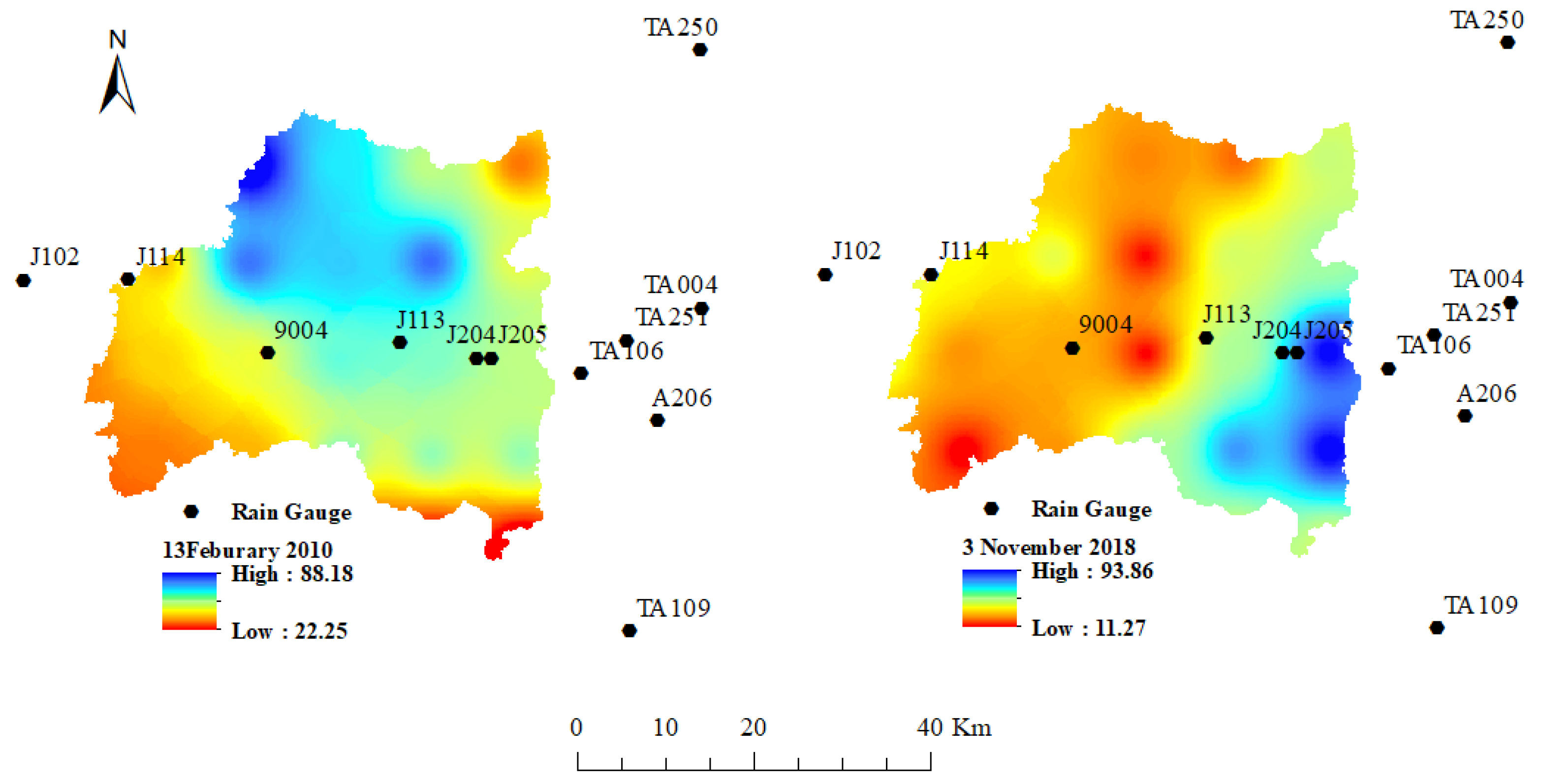
The first storm that occurred on 13 February 2010 with an average watershed total of 54.7 mm based on the Early IMERG product (Figure 2) was used for calibration. The IMERG Early product showed that the intense rainfall was concentrated over the northern portion for the 13 February 2010 event and the southeastern part of the watershed for the 3 November 2018 event. The second storm that occurred on 3 November 2018 was used for validation. Three rain gauge stations recorded the total rainfall accumulation for this event: Makkah (J114), Arafah (9004), and Muntasaf-Huda (J205), with rainfall totals of 7.8, 22.0, and 20.0 mm, respectively. The watershed-averaged total rainfall observed by the three gauges was 18.36 mm based on the Inverse Distance Squared Weighting method, while it was 42 mm based on Version 6 (Figure 2). The Early IMERG product significantly overestimated the rainfall amount for the 3 November 2018 storm event compared to observations by the ground rain gages. However, the average rainfall estimated by the Early IMERGV06 is closer to what can be inferred from a study that has been done on Wadi Al-Nu’man watershed in Makkah [29].
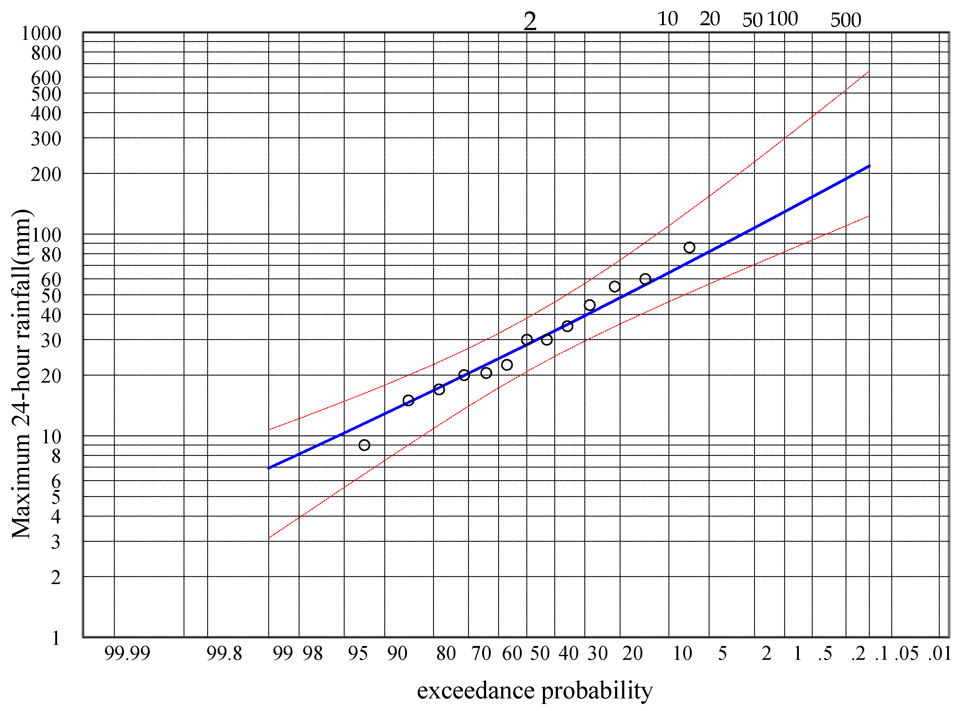
Rainfall frequency analysis was also used to estimate the rainfall for different return periods to assess the models’ performance. The recorded data from 2006 to 2018 was used to estimate the return period for maximum daily rainfall over the study area using Log-Pearson Type III distribution (LPT III) [39]. Figure 3 shows the frequency distribution as fitted to the LPT III distribution. Table 1 shows the maximum 24-h rainfall values for the return periods of 2, 5, 10, 25, 50, and 100 years.
4. Models Description
4.1. Semi-Distributed Modeling (HEC-HMS Model)
A semi-distributed model such as HEC-HMS is a compromise between a lumped model and a fully distributed one. In HEC-HMS, the watershed is divided into sub-basins to represent the watershed’s spatial heterogeneity, such as the variation of land cover/use and soil. The outputs (hydrograph, runoff volume) of the model are calculated at each sub-basin outlet and then routed downstream to estimate the hydrograph and runoff volume at the whole watershed outlet. HEC-HMS is arguably the most used model in the United States due to its flexibility, ease of use, and acceptance by almost all governmental entities. It is also one of the most popular models across the globe. The HEC-HMS model has the advantages of high-efficiency simulation, short computation times, and comparatively low calibration needs. However, it lacks the ability to consider localized effects of variation of rainfall, soil, land use, and topography [40]. In addition, the model is incapable of simulating the overland flow even at the subbasin level. Although HEC-HMS requires relatively fewer parameters for calibration, these parameters are not directly related to the watershed’s physical characteristics.
The earliest version of HEC-HMS was originally developed to simulate hydrologic processes of branched (or dendritic) watersheds [41]. The model’s software environment includes a database, computation engine, data entry utilities, and results’ reporting tools. The mathematical model used to represent the integrated watershed processes is based on a user-specified methodology (Figure 4). For example, there are eight precipitation methods to choose from, including gauge weighted average, specified hyetograph, and frequency storm. The most common method used to simulate runoff in HEC-HMS is the Soil Conservation Service (SCS) Curve Number method [11,42]. However, there are also 11 methods to choose from to determine infiltration and runoff volume, including the Curve Number and Green-Ampt.
In this study, the Curve Number (CN) loss model [43] was used to compute surface runoff. According to this method, the excess rainfall is computed according to
where Qr is the direct runoff (excess rainfall); P is the rainfall, and S (storage in the watershed) is related to the Curve Number (CN), which is computed by the following equation:
The CN values in Equation (2) range from 30 for high infiltration soils to 100 for impervious surfaces where the runoff is practically equal to rainfall. The SCS Unit Hydrograph method [44] was used to transform the excess precipitation into a runoff hydrograph using the following equations, which estimate the peak discharge (Qp) and the time to the peak discharge (tp):
where Qp = peak discharge (m3/s), Tp = the rise time of the hydrograph (hours), A = watershed area (km2), Δt = the excess duration of precipitation (hours), and tlag = lag time (hours).
The Muskingum routing method was selected in this study, and the following equation is solved by this method:
where Ot = the outflow; t = time; I = the inflow; K is the storage time constant for the reach, and X is weighing factor.
4.2. The Physically-Based, Fully Distributed Hydrologic Model (GSSHA)
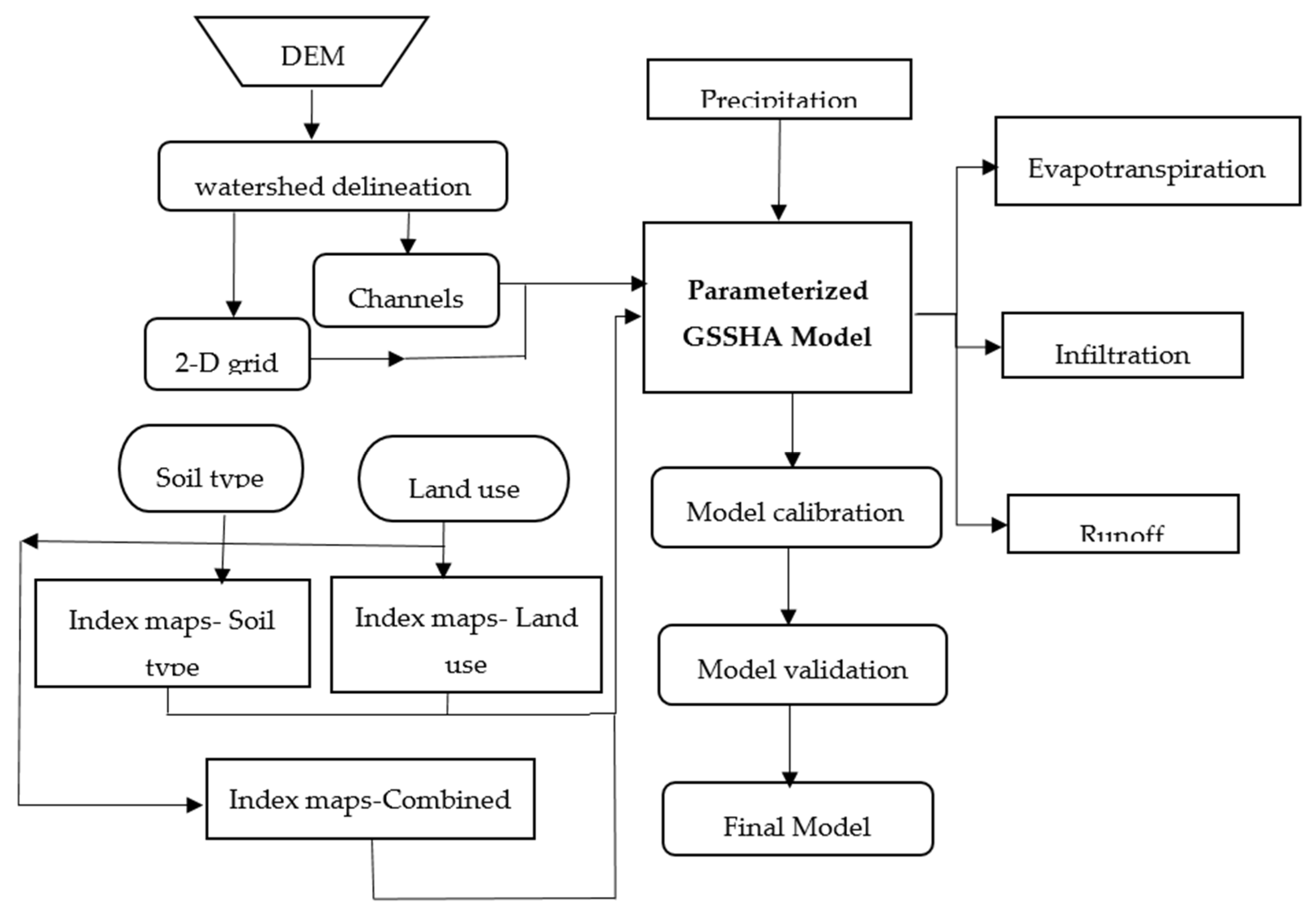
Figure 5 shows the GSSHA model set up. The GSSHA model accepts spatially variable inputs, making it very useful for evaluating land-use change effects, modeling ungauged watersheds when there is no data for calibration, and simulating the water quality and sediment yield [17,45]. In the GSSHA model, the basin is divided into grid cells considering the spatial variability of the watershed properties. The flow in every grid point can be estimated using physical equations. Accordingly, detailed hydrologic predictions at the grid-cell level across a basin can be provided by this approach. The GSSHA is a process-based model that is used to simulate channel flow (one dimension) and overland flow (two dimensions) using finite-volume solutions of the St. Venant equations of motion [46,47], and all the processes are simulated over each grid cell. The major components of the GSSHA model are: temporally and spatially varying precipitation, evapotranspiration, simplified lake storage and routing, surface runoff routing, an interception by plants, infiltration, wetland peat layer hydraulics, saturated groundwater flow, unsaturated zone soil moisture accounting, overland sediment erosion transport and deposition, overland contaminant transport and uptake, and in-stream sediment transport [48].
In GSSHA, the overland flow routing can be computed using one of three numerical techniques: ADE-Prediction Correction (PC), Explicit, and Alternative Direction Explicit (ADE). The characteristics or type of watershed will control the selection of the appropriate numerical technique. The following equation represents the ADE scheme used in this study. The inter-cell flows are calculated using Equation (6) along the x-direction:
Equation (7) is used to calculate the flow depths in each cell at the n + 1 time level based on the flows along the x-direction:
Interflows can be calculated from each cell using Equation (8) along the y-direction:
The updated column depths are calculated using Equation (9) along the y-direction based on the interflows:
where: —overland flows from cell ij in the x and y directions, respectively, —the water depth in cell ij at the nth time level, n—roughness coefficient, —the slopes of the water surface in the x and y directions, respectively, and —cell’s dimensions.
The head discharge is computed based on Manning’s equation to route the channel flow Equation (10):
where = intercell flow, n = channel roughness, Sf = the friction slope in the x-direction, A = cross section area (m2), and R = hydraulic radius. Equation (11) is used to calculate Sf.
If the effects of the backward flow are considered, the flow is calculated using the hydraulic head in the downstream cell as follows:
The volume of flow is calculated at each node using Equation (13):
where:
- = lateral flow (m2/s)
- = flow exchange between the channel and groundwater (m2/s)
- = the computed inter-cell flows from depths (h) in the longitudinal (x), at the Nth time level.
The infiltration is calculated using the GAR method as follows:
where:
- f (t) = Infiltration Rate (cm/hr)
- Sf = wetting front suction head (cm)
- K = effective hydraulic conductivity (cm/hr)
- θi = initial soil moisture content
- θs = water content of the soil at natural saturation.
5. Watershed Data
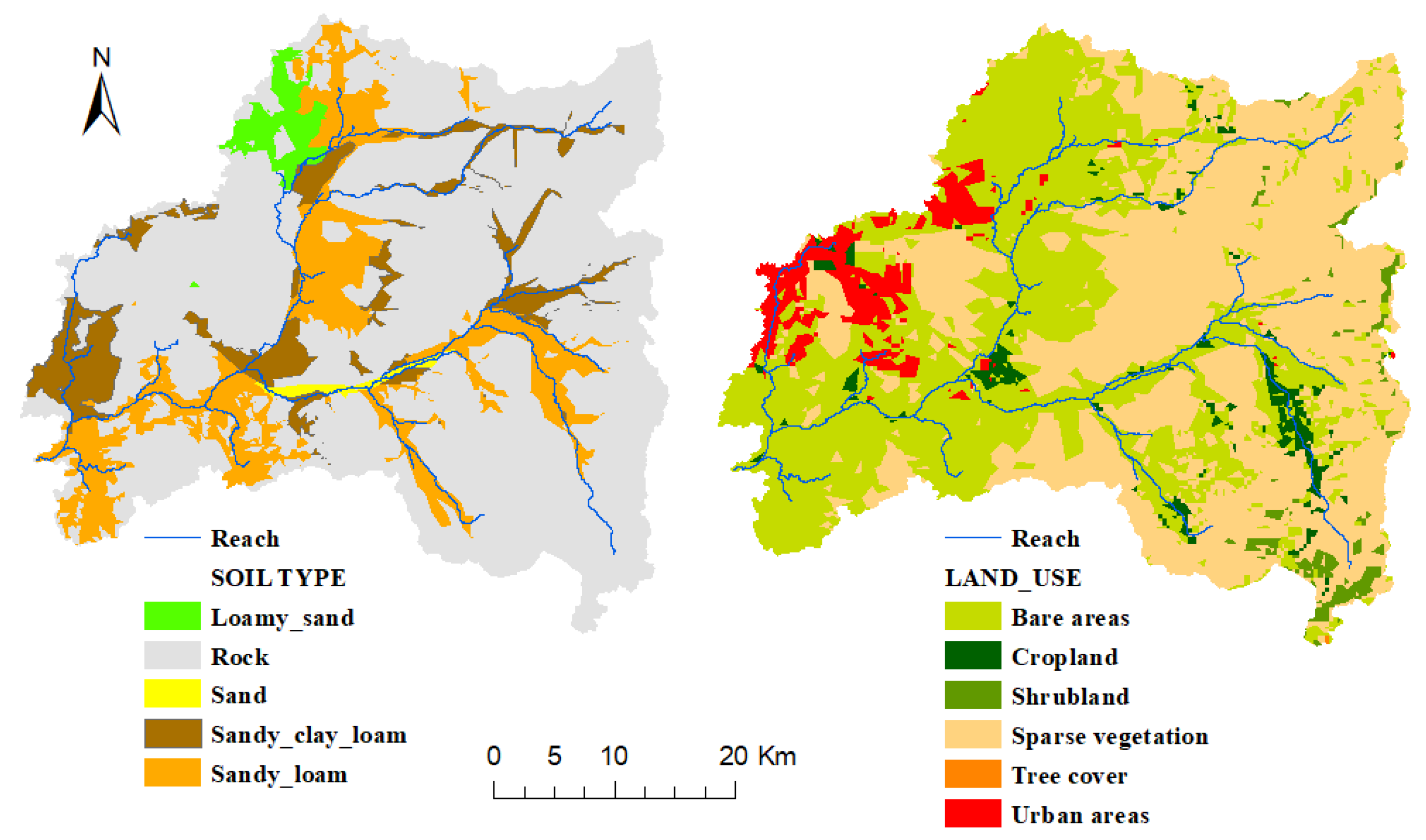
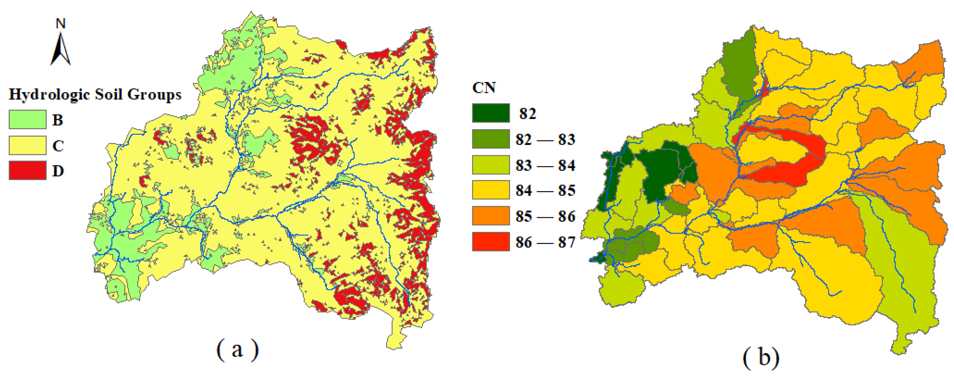
The primary input data required for the GSSHA and HEC-HMS models include rainfall data, digital elevation models (DEM), soil types, and land use/cover, which need some processing and preparation in the right input format. The DEM data, at 10 m resolution, were obtained from King Abdulaziz City of Science and Technology (KACST). The soil type data were downloaded from the SoilGridsTM global digital soil mapping system (www.SoilGrids.org (accessed on 20 March 2020)) as mass fractions of clay, silt and sand in percentages. The final soil type map (Figure 6) was developed for the Makkah watershed using ArcGIS10.6 [49], and the soil texture classification based on the clay, silt, and sand contents and then adjusted after comparison with aerial photographs and field information. The land use/cover data (Figure 6) were obtained from the OpenLandMap data portal (www.openlandmap.org (accessed on 25 March 2020)), and adjustments were made after comparison with aerial photographs. The hydrologic soil group data were obtained from the HYSOGs250m product ([50] https://daac.ornl.gov/SOILS/guides/Global_Hydrologic_Soil_Group.html (accessed on 26 March 2020)) at 250 m resolution as shown in Figure 7a. This data were used to estimate the CN values (Figure 7b) needed for the HEC-HMS model.
6. Methodology
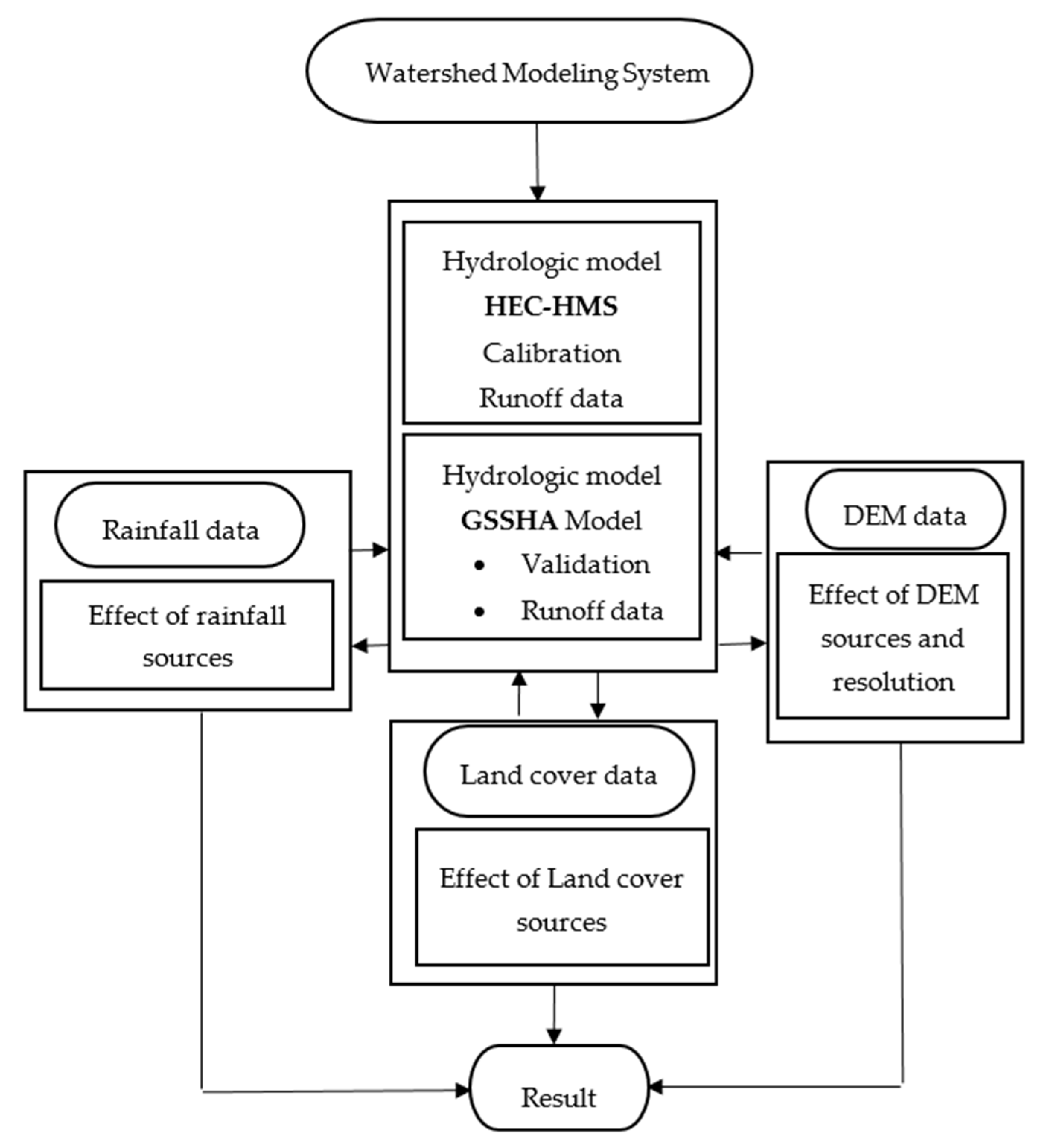
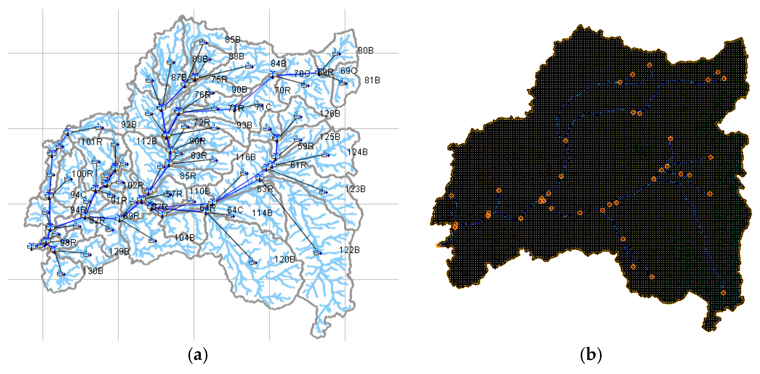
The methodology adopted in this study is described through the flowchart shown in Figure 8. ArcGIS 10.6 was used to prepare the raster data for WMS [51] to be processed and exported to HEC-HMS. The process in WMS includes delineation of the watershed, flow accumulations, flow directions, and computing CN values based on the hydrologic groups in Figure 7. The watershed was subdivided into 55 sub-basins for HEC-HMS simulations, as shown in Figure 9a. The SCS Curve Number and SCS dimensionless transformation methods were applied to compute the runoff volumes and to model direct runoff, respectively, while the Muskingum method was used for channel routing. The inverse distance method was used to generate the rainfall hyetograph for the selected storm events before being used as input to the HEC-HMS model.
The channel roughness, channel cross-sections, and other parameters such as hydraulic conductivity were required for the GSSHA model. ArcGIS and WMS were also used to prepare the raster data for the GSSHA model. All streams were smoothed to avoid the effect of the adverse and flat slopes resulting from inaccuracies in the DEM. The watershed was divided into grid cells at 150 × 150 m resolution (Figure 9b). The land use/cover and soil types were imported by WMS to prepare the grid index maps which then were used to estimate the required parameters such as infiltration parameters, roughness, initial moisture, overland retention depth, and impervious fraction. The WMS was also used to extract channel cross-sections from the 10 m DEM (Figure 10). The no-flow condition was adopted for all first-order streams boundary conditions in GSSHA as there is no baseflow in the basin [47].
7. Results
7.1. Models Calibration
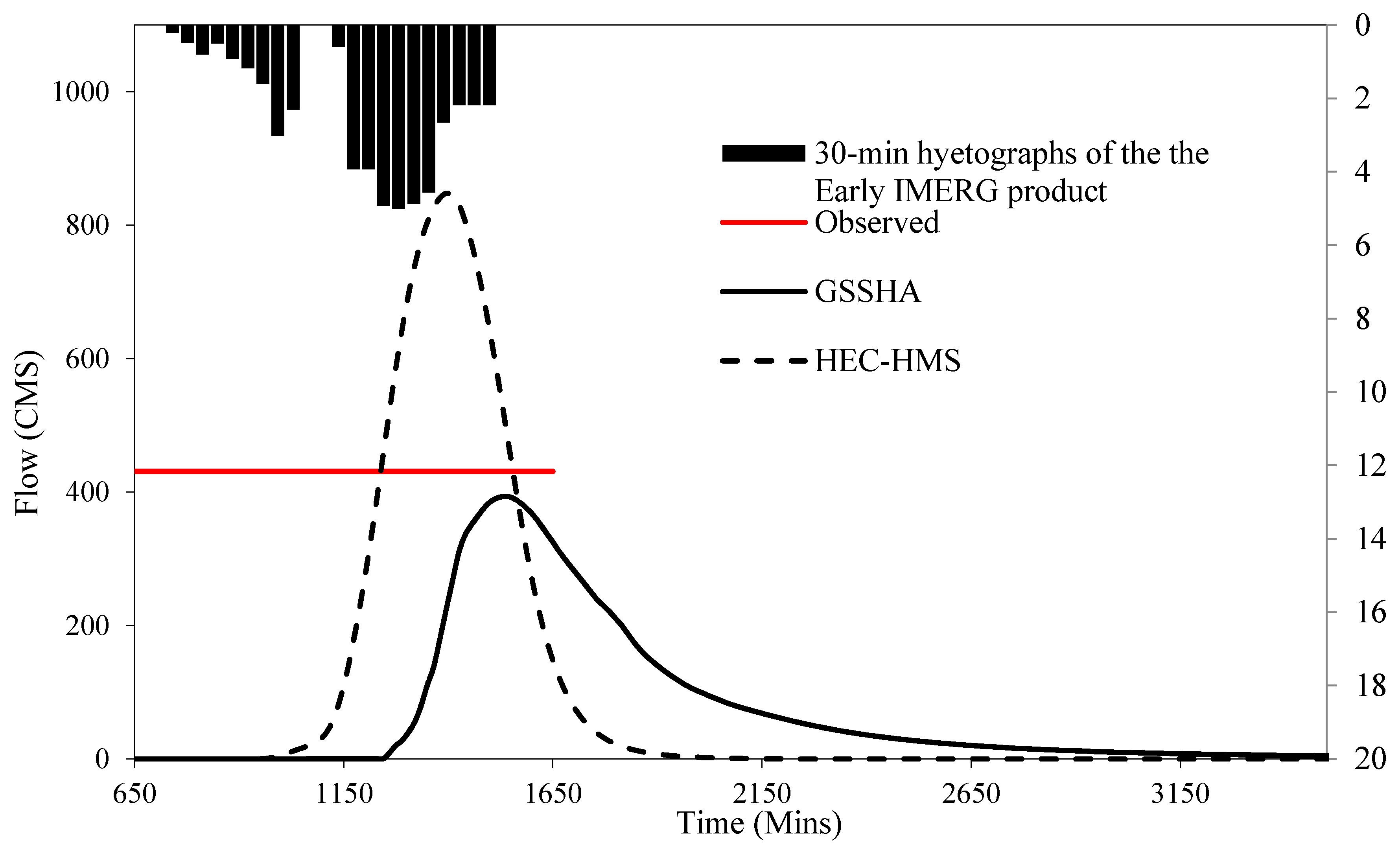
The storm event of 13 February 2010 with total rainfall accumulation of 55 mm resulting in a peak discharge of 431 m3/s and a flow depth of 1.6m measured at a point of intersection between Wadi Uranah (610.8 km2) and Mashar Arafat [52] was used to calibrate both the GSSHA and HEC-HMS models. Since HEC-HMS is not a fully distributed model, each IMERG rainfall grid value was input to the HEC-HMS as point observation at the grid center, and this process was applied over the whole watershed. The rainfall hyetograph for each sub-basin for the selected storm event was generated using the Thiessen Polygons method. On the other side, GSSHA can accept temporally and spatially varying precipitation from a satellite. A time step of 15-min was used for the discharge output for the two models. Figure 11 shows the simulated hydrographs from HEC-HMS and GSSHA simulations before calibration. It can be noticed that HEC-HMS significantly overestimated the observed peak discharge, while the GSSHA model slightly underestimated the observed peak discharge. Accordingly, the HEC-MS was calibrated by adjusting the CN values and Muskingum parameters and the GSSHA model by adjusting the hydraulic conductivity and roughness values.
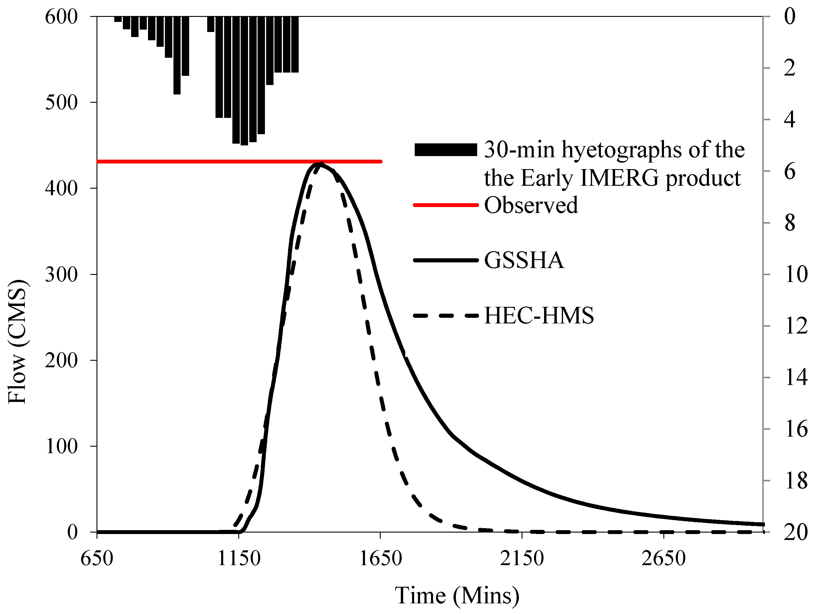
Both models produced acceptable hydrographs after calibration, as shown in Figure 12. However, the runoff volume produced by HEC-HMS after calibration was smaller by 38% than that produced by GSSHA. In other words, the percentage of losses due to infiltration that resulted from HEC-HMS (73.6%) is more than that for GSSHA (57.5%). We could not verify the two models’ runoff volume since the observed runoff volume was not available. It can be seen from Figure 12 that the base time of the hydrograph simulated by GSSHA is much greater than that for HEC-HMS. This could be attributed to the significant effect of the grid cells in the distributed model, representing the spatial variability of the watershed properties more accurately. On the other hand, the basin is divided into sub-basins in the HEC-HMS model, and the surface slope is taken as the average for each sub-basin. This cannot accurately represent the real conditions, especially in complex terrain dominated by mountains with steep slopes such as Makkah watershed, where the average slope masks the effect of relief variability.
7.2. Models’ Validation
The HEC-HMS and GSSHA models were validated using the storm event of 3 November 2018 when a peak discharge of 640–680 m3/s was estimated at three points in the main channel near the outlet of Wadi Al-Nu’man, which has a drainage area of 683.4 km2 (Figure 1). These estimates were based on a maximum flow depth of about 3.5 to 4 m measured by observers from the University of Umm Al-Qura and a consulting company [28]. The observed runoff hydrograph could not be reconstructed because the flow depth and peak discharge values were the only available observed data. Moreover, there is no information about the peak discharge timing and hydrograph duration. Accordingly, we used one statistic measure in model validation, which is the error in peak discharge (εp) using the following equation:
where: Po is the observed peak discharge; Ps is the simulated peak discharge.
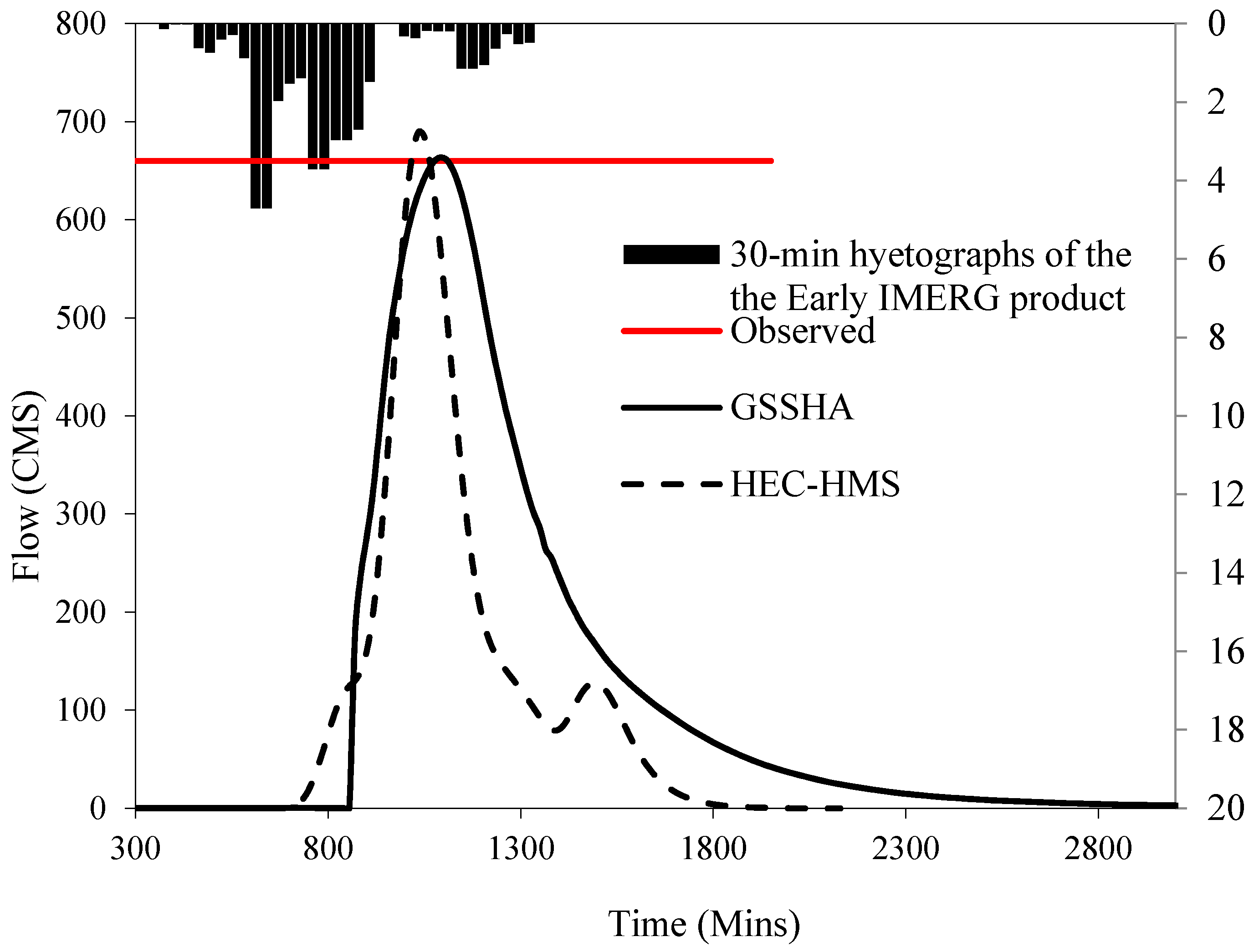
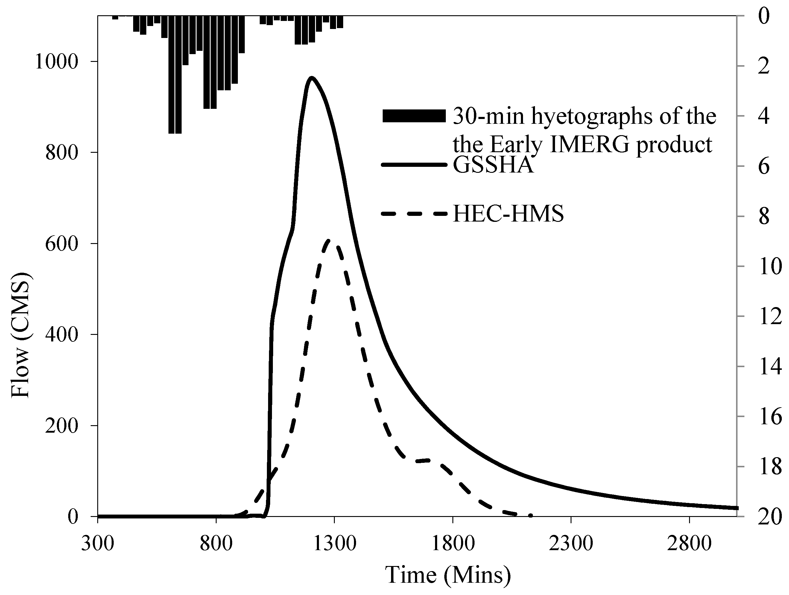
When using the IMERG Early run product as input, HEC-HMS overestimated the peak by 4.5%, while GSSHA overestimated the peak by just under 1% (Table 2 and Figure 13). However, the estimated runoff volume and the percentage of infiltration losses estimated by the two models were quite different. Again, the runoff volume estimated by HEC-HMS is much lower than the GSSHA estimate. This may indicate that HEC-HMS was not able to represent the complex topography of the study area.
7.3. Models’ Outputs Comparison
Figure 14 and Figure 15 show the hydrographs simulated by the two models at the entire Makkah watershed outlet. The outlet peak discharge values produced by HEC-HMS for calibration and validation events were lower than those produced by the GSSHA model by 16.3% and 36.7%, respectively. For the 2010 and 2018 storm events, the HEC-HMS model estimated runoff ratios of 21.2% and 18.9%, respectively, while the runoff ratios calculated by GSSHA were 39% and 41.5%, respectively.
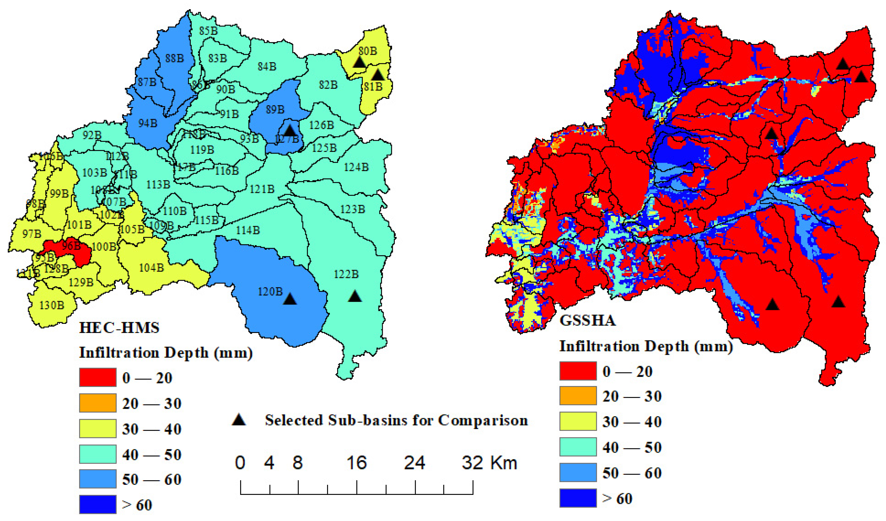
Unlike HEC-HMS, GSSHA provides distributed outputs of major hydrologic states and fluxes such as infiltration, runoff at high temporal and spatial resolutions, and soil moisture as maps. However, each sub-basin’s infiltration values can be estimated from HEC-HMS sub-basin results. These values can be used to develop average infiltration depth maps using GIS. Figure 16 shows maps of the cumulative infiltration depths (m) produced by HEC-HMS and GSSHA. The figure highlights the significant difference between the estimates of the two models. In HEC-HMS, the average infiltration is calculated by considering the whole sub-basin as one unit, while in GSSHA, the infiltration is calculated for each grid cell. As a result, the uniform infiltration over each sub-basin is not realistic. The GSSHA infiltration map shows the infiltration in limited areas, around the main channels, and in the flat areas with the soil of high hydraulic conductivity, which could be closer to the real conditions. In addition, the GSSHA infiltration map shows very low infiltration depth values over the mountains because of the low hydraulic conductivity and steep slopes. In contrast, the HEC-HMS map shows higher infiltration depths over these areas.
The GSSHA model has the ability to estimate all model outputs at any location inside the basin. To compare the two models’ outputs at the sub-basin scale, we allow GSSHA to estimate output hydrographs at points that coincide with some selected HEC-HMS sub-basins outlets. The locations of the points selected for comparison are shown in Figure 16. The comparison statistics are shown in Table 3. The table shows that the peak discharges estimated by HEC-HMS are 26.9 to 78.5% lower than the GSSHA estimates, while the runoff volumes are lower by 59.5 to 92.9%. This significant difference between the two models can be attributed to several reasons. For example, HEC-HMS produced high infiltration values for the sub-basins 80B and 81B, located in the upper right portion of the basin, whereas the GSSHA model produced very low infiltration resulting in huge differences in the peak discharge and runoff volume, as shown in Table 3. Sub-basin 120B includes one of the widest channels underlain by highly permeable soils. For this sub-basin, GSSHA estimated high infiltration values mostly in and around the channels, as shown in Figure 16, while the whole sub-basin was subjected to high infiltration as shown in the HEC-HMS map. This comparison confirms that the calibration and validation at one location do not lead to an agreement of the results of the two models over the entire watershed, especially for large watersheds. As a result, several locations for model calibration and validation are required. However, in case of the difficulties of getting the required data, the calibration/validation at the location of the existing/suggested hydraulic structure will still be valuable.
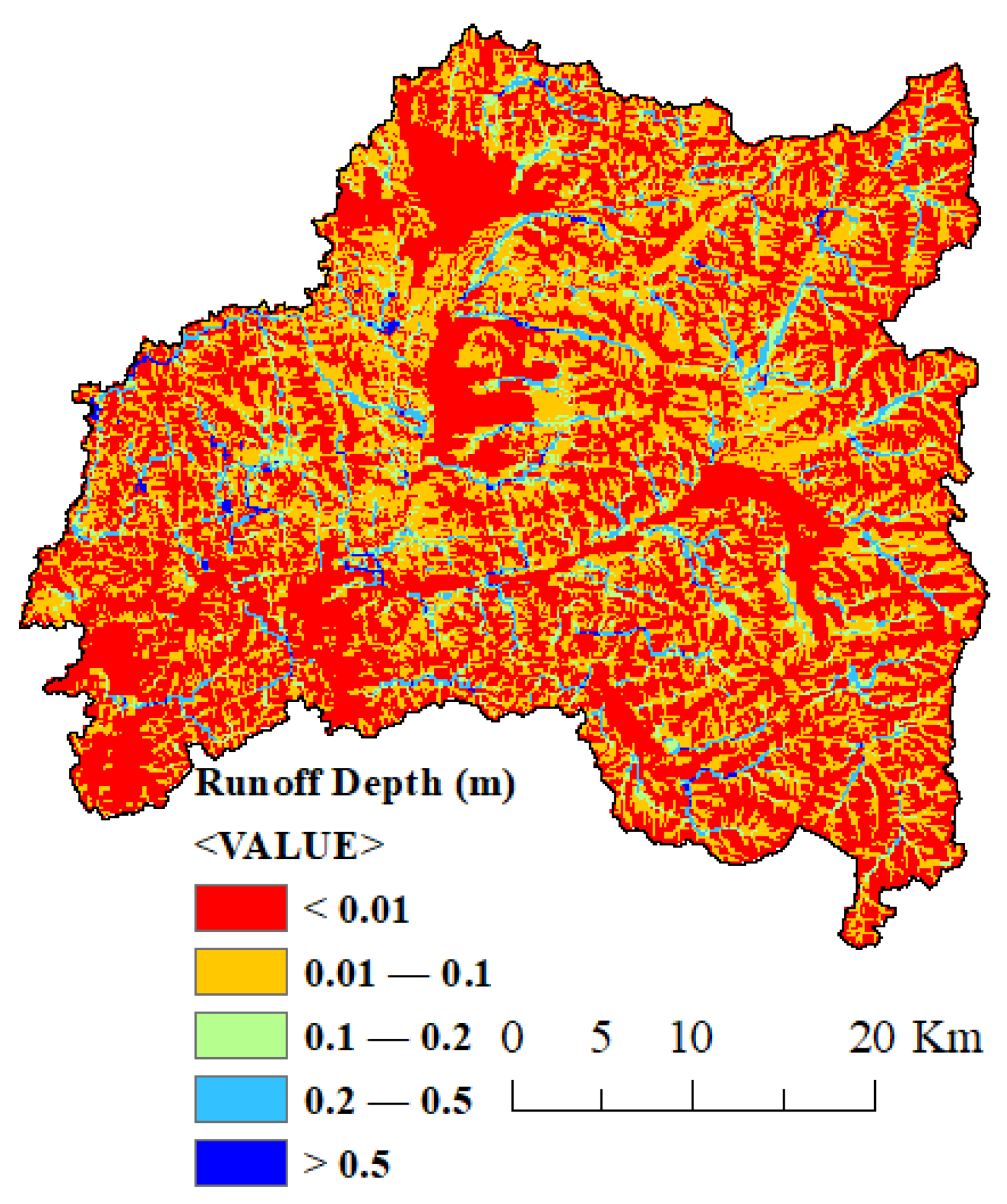
A major advantage of the GSSHA model is its capability to simulate infiltration for small subsegments of the watershed. This can help to identify areas within the watershed with high infiltration and consequently can help to determine locations within the watershed where excess runoff for managed aquifer recharge and prevent flooding without costly structural measures can be utilized. Figure 17 shows the distributed runoff depths. The detailed information on runoff depths produced by the GSSHA model can be utilized to guide innovative flood mitigation and countermeasures in the urbanized portions of the watershed and even traffic planning and rescue efforts during extreme events.
7.4. Effect of Topography on HEC-HMS Simulations
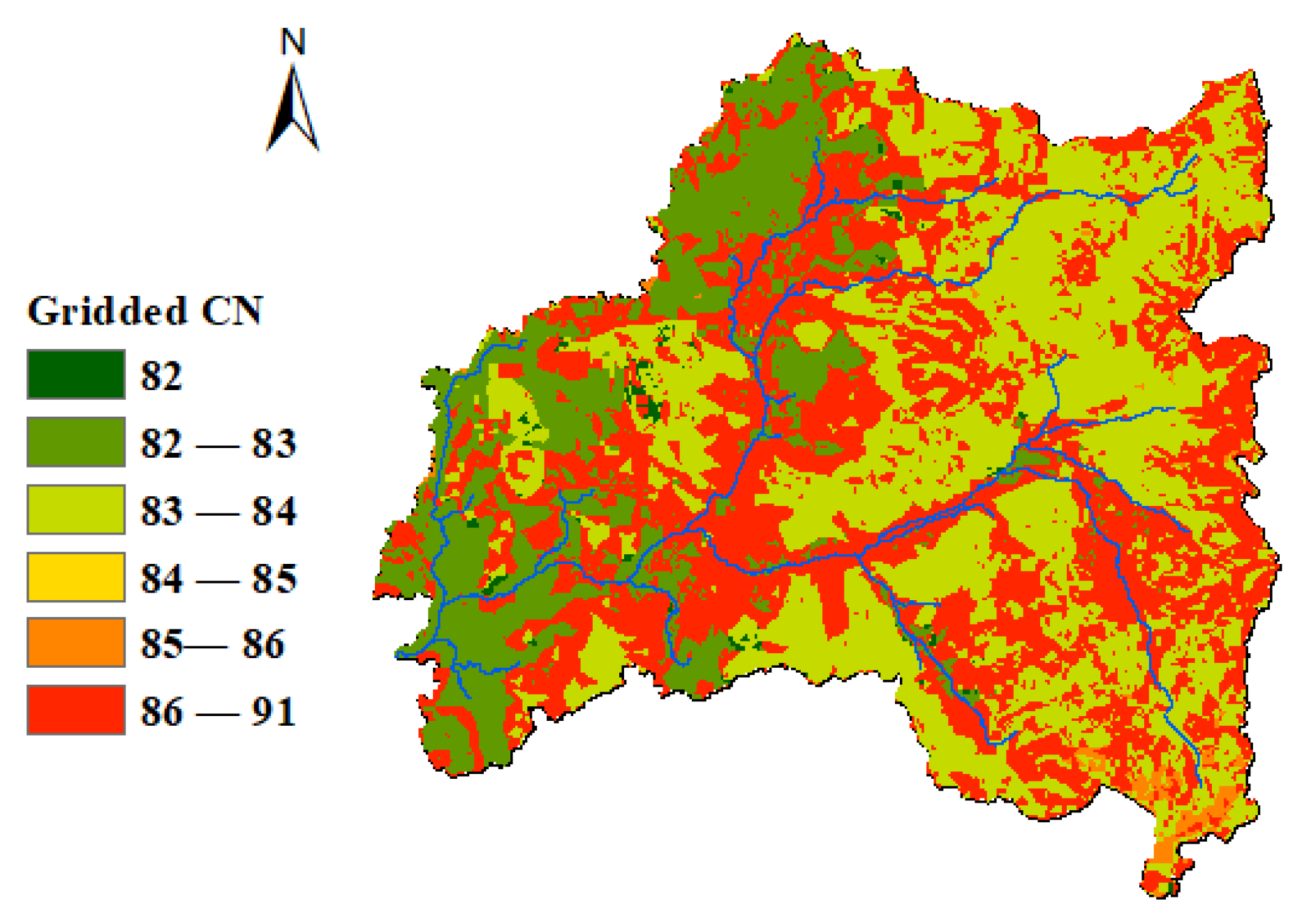
To gain more understanding of the effect of complex topography and spatial heterogeneity of the study area on the model predictions, GSSHA and three models of HEC-HMS were used to estimate the outlet hydrograph for the whole Makkah watershed. The ModClark approach, one of many rainfall-runoff methods in HEC-HMS, provides an advanced feature for gridded runoff simulation. The ModClark approach is based on Clark’s Unit Hydrograph [53]. It employs a grid representation that makes it convenient for applying a gridded CN method. This helps examine the effect of the study area’s complex topography on the output hydrograph using the same input data of the semi-distributed models. Two different versions of the semi-distributed model were also used. One is based on the SCS unit hydrograph (SCS-UH), and the other one is based on the Clark Unit Hydrograph (CU-H). The basin lag time is the main parameter of SCS-UH, while the time of concentration (tc) and a storage coefficient (R) are the main parameters of C-UH. The Muskingum method was used for channel routing for all HEC-HMS models. The three models (semi-distributed (SCS-UH), semi-distributed (CUH), and ModClark) were prepared with the same input data, while GSSHA was prepared with the same minimum required input data. Since the objective was only to show the effect of watershed heterogeneity, Type II storm distribution with a return period of 10 years was used as input to the four rainfall-runoff models. Figure 18 shows the gridded CN map developed for the ModClark model, which is significantly different from the sub-basins based CN map (see Figure 7). Table 4 summarizes the modeling approach used.
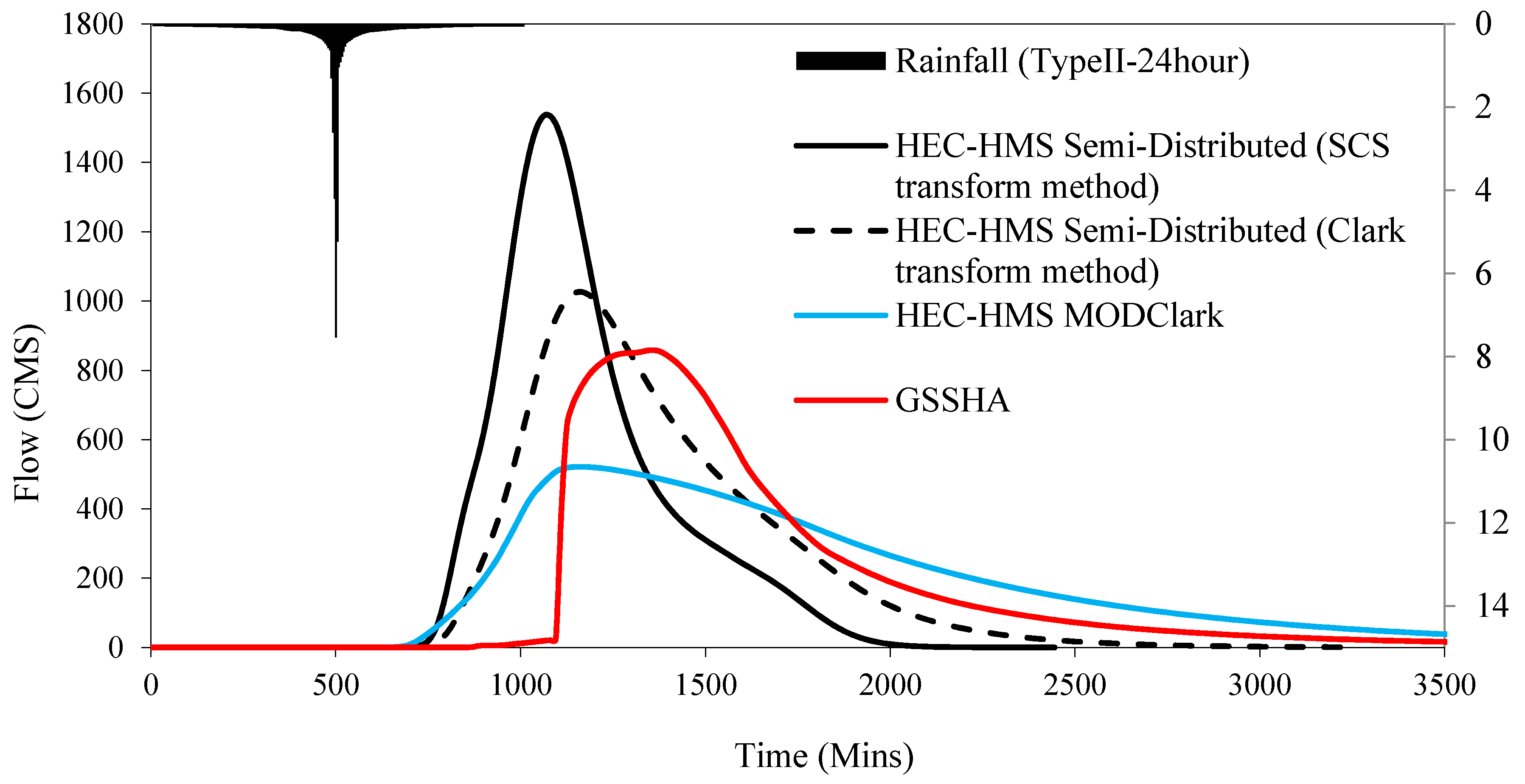
It can be noticed from Figure 19 that the hydrograph base time produced by GSSHA and HEC-HMS ModClark are much greater than those produced by the semi-distributed models with the (SCS-UH) model estimating the shortest base time. In addition, it can be seen in Figure 19 and Table 5 that the peak discharge produced by GSSHA is greater than that for HEC-HMS ModClark and less than that produced by other HEC-HMS models. The difference in the peak discharge between the semi-distributed (SCS-UH) and (C-UH) models can be attributed to the difference in the unit hydrograph assumptions.
With the same input data, loss method, transform method, and channel routing, the semi-distributed (C-UH) and ModClark models are almost identical except in that ModClark is a distributed model [54]. Thus, the difference in results can be primarily attributed to the study area’s complex topography. The difference in the peak discharge between the semi-distributed (C-UH) and ModClark models (Figure 19 and Table 5) is due to ModClark discretization of the watershed into smaller grid cells, resulting in an increase in the travel time reflecting the effect of the complex topography of the study area. This demonstrates the impact of the study area’s complex topography that can not be represented very well by the lumped or semi-distributed HEC-HMS models. However, the GSSHA model produced higher peak discharge than the ModClark model, which could be attributed to the difference in the modeling methods (Table 5). Halwatura & Najim [55] found that the performance of the SCS-CN was not satisfactory in many cases. Walega et al. [56] found that the prediction of direct runoff by modified Sahu-Mishra-Eldho—curve number (SME-CN) is much more accurate than the original SCS-CN method implemented in HEC-HMS.
8. Conclusions
In this study, a physically-based, fully distributed model (GSSHA) and a conceptual semi-distributed model (HEC-HMS) were used to simulate flood events over an arid watershed in Makkah, Saudi Arabia. The steep slopes and large fraction of impervious surfaces of the study area increase drainages efficiency and contribute to the occasional flash floods in the city. Hydrographs simulated by the two models were compared to observed peak discharge for one flood event using satellite rainfall as input. One more event was used for model validation. The two models were prepared with the minimum required data so that the comparison between the two models would be meaningful. The performance of the models was measured by the peaks’ discharge. The effort required to build the two models was comparable since the same input data were used, and a similar number of parameters were calibrated. However, additional effort was needed to define channel cross-sections for the GSSHA model. Moreover, cell-to-cell surface runoff computations in GSSHA required more time than did the lower resolution sub-basin runoff computations of HEC-HMS.
Although the GSSHA model performed better than HEC-HMS, which significantly overestimated the peak discharge before calibration, the two models’ performance after calibration was comparable. However, the runoff volumes produced by HEC-HMS were much smaller than GSSHA for all calibration and validation events. The failure of HEC-HMS to capture details of the complex terrain and land surface heterogeneity was likely behind this discrepancy. The cell-to-cell routing of flow that was only possible with GSSHA. The GSSHA model can make use of higher-resolution DEMs and rainfall products that are becoming more available and are more suitable in urban areas, where the natural landscape is significantly modified.
The difference in the output of GSSHA and HEC-HMS was investigated further by comparing GSSHA hydrograph to those produced using three implementations of HEC-HMS (semi-distributed (SCS-UH), semi-distributed (C-UH), and ModClark). A uniform design storm was used as input. The two semi-distributed (SCS-UH and C-UH) models were implemented with the same input data, losses method, and routing. The results showed that the semi-distributed (C-UH) model produced less peak discharge than the semi-distributed (SCS-UH) one. This could be related to the effect of the storage coefficient in the C-UH model, which is geomorphological data and unique for each watershed. The HEC-HMS ModClark model hydrograph was comparable to that of GSSHA, indicating that it was able to capture the effect of the complex topography of the watershed. The comparison results were intended only for situations when a quick and simple hydrologic model simulation is to be performed. All models could have been built more deliberately by incorporating more of the watershed features, such as the detention/retention structure in residential areas, if observed runoff data were available. This can be investigated in more detail in future studies.
A major advantage of the GSSHA model is that the detailed information on high infiltration areas produced by the model can help identify the locations where the excess runoff can be utilized in aquifer recharge. This can help reduce flooding without the need for costly structural measures. Moreover, the detailed information on the runoff depths produced by the GSSHA can be used for designing flood control structures and other planning purposes.
Author Contributions
A.M.A.-A., M.A.A.-Z. and H.O.S. developed the research methodology, M.A.A.-Z. guided this research, and contributed significantly to the preparation of the manuscript for publication. A.M.A.-A. downloaded and processed the remote sensing products. A.M.A.-A. and M.A.A.-Z. developed the model and performed calibration and validation. A.M.A.-A. prepared the first draft. M.A.A.-Z. and H.O.S. performed the final overall proofreading of the manuscript. All authors have read and agreed to the published version of the manuscript.
Funding
This research received no external funding.
Acknowledgments
The authors wish to acknowledge the support of King Fahd University of Petroleum and Minerals (KFUPM) in conducting this research.
Conflicts of Interest
The authors declare no conflict of interest.
References
- Zhao, Q.; Ding, Y.; Wang, J.; Gao, H.; Zhang, S.; Zhao, C.; Xu, J.; Han, H.; Shangguan, D. Projecting Climate Change Impacts on Hydrological Processes on the Tibetan Plateau with Model Calibration against the Glacier Inventory Data and Observed Streamflow. J. Hydrol. 2019, 573, 60–81. [Google Scholar] [CrossRef]
- Umair, M.; Kim, D.; Ray, R.L.; Choi, M. Estimating Land Surface Variables and Sensitivity Analysis for CLM and VIC Simulations Using Remote Sensing Products. Sci. Total Environ. 2018, 633, 470–483. [Google Scholar] [CrossRef]
- Santos, R.M.B.; Sanches Fernandes, L.F.; Moura, J.P.; Pereira, M.G.; Pacheco, F.A.L. The Impact of Climate Change, Human Interference, Scale and Modeling Uncertainties on the Estimation of Aquifer Properties and River Flow Components. J. Hydrol. 2014, 519, 1297–1314. [Google Scholar] [CrossRef]
- Zhang, Z.; Koren, V.; Smith, M.; Reed, S.; Wang, D. Use of Next Generation Weather Radar Data and Basin Disaggregation to Improve Continuous Hydrograph Simulations. J. Hydrol. Eng. 2004, 9, 103–115. [Google Scholar] [CrossRef] [Green Version]
- Furl, C.; Ghebreyesus, D.; Sharif, H.O. Assessment of the Performance of Satellite-Based Precipitation Products for Flood Events across Diverse Spatial Scales Using GSSHA Modeling System. Geosciences 2018, 8, 191. [Google Scholar] [CrossRef] [Green Version]
- Al-Zahrani, M.; Al-Areeq, A.; Sharif, H.O. Estimating Urban Flooding Potential near the Outlet of an Arid Catchment in Saudi Arabia. Geomat. Nat. Hazards Risk 2017, 8, 672–688. [Google Scholar] [CrossRef] [Green Version]
- Reed, S.; Koren, V.; Smith, M.; Zhang, Z.; Moreda, F.; Seo, D.-J. DMIP Participants, and Overall Distributed Model Intercomparison Project Results. J. Hydrol. 2004, 298, 27–60. [Google Scholar] [CrossRef]
- Biftu, G.; Gan, T. Semi-Distributed, Physically Based, Hydrologic Modeling of the Paddle River Basin, Alberta, Using Remotely Sensed Data. J. Hydrol. 2001, 244, 137–156. [Google Scholar] [CrossRef]
- Refsgaard, J.C. Parameterisation, Calibration and Validation of Distributed Hydrological Models. J. Hydrol. 1997, 198, 69–97. [Google Scholar] [CrossRef]
- Donnelly-Makowecki, L.; Moore, R. Hierarchical Testing of Three Rainfall–Runoff Models in Small Forested Catchments. J. Hydrol. 1999, 219, 136–152. [Google Scholar] [CrossRef]
- Shrestha, M.N. Spatially Distributed Hydrological Modelling Considering Land–Use Changes Using Remote Sensing and GIS. In Proceedings of the Map Asia Conference, Kuala Lumpur, Malaysia, 13–15 October 2003. [Google Scholar]
- Bobba, A.G.; Singh, V.P.; Bengtsson, L. Application of Environmental Models to Different Hydrological Systems. Ecol. Modell. 2000, 125, 15–49. [Google Scholar] [CrossRef]
- Schumann, A.H. Development of Conceptual Semi-Distributed Hydrological Models and Estimation of Their Parameters with the Aid of GIS. Hydrol. Sci. J. 1993, 38, 519–528. [Google Scholar] [CrossRef]
- Jones, J.A.A. Global Hydrology: Processes, Resources and Environmental Management; Routledge: Oxfordshire, UK, 2014; ISBN 9781315844398. [Google Scholar]
- Vázquez, R.F.; Feyen, L.; Feyen, J.; Refsgaard, J.C. Effect of Grid Size on Effective Parameters and Model Performance of the MIKE-SHE Code. Hydrol. Process. 2002, 16, 355–372. [Google Scholar] [CrossRef]
- Sharif, H.O.; Sparks, L.; Hassan, A.A.; Zeitler, J.; Xie, H. Application of a Distributed Hydrologic Model to the November 17, 2004, Flood of Bull Creek Watershed, Austin, Texas. J. Hydrol. Eng. 2010, 15, 651–657. [Google Scholar] [CrossRef]
- Paudel, M.; Nelson, E.J.; Downer, C.W.; Hotchkiss, R. Comparing the Capability of Distributed and Lumped Hydrologic Models for Analyzing the Effects of Land Use Change. J. Hydroinformatics 2011, 13, 461–473. [Google Scholar] [CrossRef]
- Sith, R.; Nadaoka, K. Comparison of SWAT and GSSHA for High Time Resolution Prediction of Stream Flow and Sediment Concentration in a Small Agricultural Watershed. Hydrology 2017, 4, 27. [Google Scholar] [CrossRef] [Green Version]
- Zhang, H.L.; Zhang, H.L.; Wang, Y.J.; Wang, Y.Q.; Li, D.X.; Wang, X.K. Quantitative Comparison of Semi- and Fully-Distributed Hydrologic Models in Simulating Flood Hydrographs on a Mountain Watershed in Southwest China. J. Hydrodyn. 2013, 25, 877–885. [Google Scholar]
- El-Nasr, A.A.; Arnold, J.G.; Feyen, J.; Berlamont, J. Modelling the Hydrology of a Catchment Using a Distributed and a Semi-Distributed Model. Hydrol. Process. 2005, 19, 573–587. [Google Scholar] [CrossRef]
- Meselhe, E.A.; Habib, E.H.; Oche, O.C.; Gautam, S. Sensitivity of Conceptual and Physically Based Hydrologic Models to Temporal and Spatial Rainfall Sampling. J. Hydrol. Eng. 2009, 14, 711–720. [Google Scholar] [CrossRef]
- Ogden, F.L.; Downer, C.W.; Meselhe, E. U.S. Army Corps of Engineers Gridded Surface/Subsurface Hydrologic Analysis (GSSHA) Model: Distributed-Parameter, Physically Based Watershed Simulations. In Proceedings of the World Water & Environmental Resources Congress 2003, Philadelphia, PA, USA, 23–26 June 2003; American Society of Civil Engineers: Reston, VA, USA, 2003; pp. 1–10. [Google Scholar]
- El Hassan, A.A.; Sharif, H.O.; Jackson, T.; Chintalapudi, S. Performance of a Conceptual and Physically Based Model in Simulating the Response of a Semi-Urbanized Watershed in San Antonio, Texas. Hydrol. Process. 2013, 27, 3394–3408. [Google Scholar] [CrossRef]
- Al Abdouli, K.; Hussein, K.; Ghebreyesus, D.; Sharif, H.O. Coastal Runoff in the United Arab Emirates-the Hazard and Opportunity. Sustainability 2019, 11, 5406. [Google Scholar] [CrossRef] [Green Version]
- Sharif, H.; Al-Zahrani, M.; Hassan, A. Physically, Fully-Distributed Hydrologic Simulations Driven by GPM Satellite Rainfall over an Urbanizing Arid Catchment in Saudi Arabia. Water 2017, 9, 163. [Google Scholar] [CrossRef]
- Embaby, A.; Halawa, A.A.; Ramadan, M. Integrating Geotechnical Investigation with Hydrological Modeling for Mitigation of Expansive Soil Hazards in Tabuk City, Saudi Arabia. Mod. Hydrol. 2017, 7, 11–37. [Google Scholar] [CrossRef] [Green Version]
- Fathy, I.; Negm, A.M.; El-fiky, M.; Nassar, M.; El-Sayed, E.A.H. Runoff Hydrograph Modeling for Arid Regions: Case Study—Wadi Sudr-Sinai. Int. Water Technol. J. IWTJ 2015, 5, 58–68. [Google Scholar]
- Abdelkarim, A.; Gaber, A.F.D. Flood Risk Assessment of the Wadi Nu’man Basin, Mecca, Saudi Arabia (During the Period, 1988–2019) Based on the Integration of Geomatics and Hydraulic Modeling: A Case Study. Water 2019, 11, 1887. [Google Scholar] [CrossRef] [Green Version]
- Elfeki, A.; Masoud, M.; Niyazi, B. Integrated Rainfall–Runoff and Flood Inundation Modeling for Flash Flood Risk Assessment under Data Scarcity in Arid Regions: Wadi Fatimah Basin Case Study, Saudi Arabia. Nat. Hazards 2017, 85, 87–109. [Google Scholar] [CrossRef]
- El Bastawesy, M.; Habeebullah, T.; Balkhair, K.; Ascoura, I. Modelling Flash Floods in Arid Urbanized Areas: Makkah (Saudi Arabia). Sécheresse 2013, 24, 171–181. [Google Scholar] [CrossRef]
- Dawod, G.M.; Mirza, M.N.; Al-Ghamdi, K.A. Assessment of Several Flood Estimation Methodologies in Makkah Metropolitan Area, Saudi Arabia. Arab. J. Geosci. 2013, 6, 985–993. [Google Scholar] [CrossRef]
- Al-ghamdi, K.A.; Elzahrany, R.A.; Mirza, M.N.; Dawod, G.M. Impacts of Urban Growth on Flood Hazards in Makkah City, Saudi Arabia. Int. J. Water Resour. Environ. Eng. 2012, 4, 23–34. [Google Scholar]
- Al Saud, M. Morphometric Analysis of Wadi Aurnah Drainage System, Western Arabian Peninsula. Open Hydrol. J. 2009, 3, 1–10. [Google Scholar]
- GAS Population. Available online: https://www.stats.gov.sa/en/852 (accessed on 31 August 2020).
- Subyani, A.M. Hydrologic Behavior and Flood Probability for Selected Arid Basins in Makkah Area, Western Saudi Arabia. Arab. J. Geosci. 2011, 4, 817–824. [Google Scholar] [CrossRef]
- Alahmadi, M.; Atkinson, P.M. Three-Fold Urban Expansion in Saudi Arabia from 1992 to 2013 Observed Using Calibrated DMSP-OLS Night-Time Lights Imagery. Remote Sens. 2019, 11, 2266. [Google Scholar] [CrossRef] [Green Version]
- Al Jabri, N.; Alhazmi, R. Observing and Monitoring the Urban Expansion of Makkah Al-Mukarramah Using the Remote Sensing and GIS. J. Eng. Sci. Inf. Technol. 2017, 1, 103–125. [Google Scholar]
- Tan, J.; Huffman, G.J.; Bolvin, D.T.; Nelkin, E.J. IMERG V06: Changes to the Morphing Algorithm. J. Atmos. Ocean. Technol. 2019, 36, 2471–2482. [Google Scholar] [CrossRef]
- Chow, V.T. A General Formula for Hydrologic Frequency Analysis. Trans. Am. Geophys. Union 1951, 32, 231. [Google Scholar] [CrossRef]
- Lautenbach, S.; Voinov, A.; Seppelt, R. Localization Effects of Land Use Change on Hydrological Models. In Proceedings of the iEMSs Third Biennial Meeting, Summit on Environmental Modelling and Software, Burlington, VT, USA, 9–13 July 2006; Voinov, A., Jakeman, A., Rizzoli, A., Eds.; International Environmental Modelling and Software Society: Burlington, VT, USA, 2006. [Google Scholar]
- Scharffenberg, W.A. Hydrologic Modeling System HEC-HMS–User’s Manual; Institute for Water Resources, Hydrologic Engineering Center: Davis, CA, USA, 2013; p. 442. [Google Scholar]
- Mishra, S.K.; Singh, V. Soil Conservation Service Curve Number (SCS-CN) Methodology; Springer Science & Business Media: Berlin/Heidelberg, Germany, 2003; p. 513. [Google Scholar]
- Urban Hydrology for Small Watersheds; No. 55. Engineering Division, Soil Conservation Service, US Department of Agriculture: Washington, DC, USA, 1986.
- Kent, K.M. Section 4–Hydrology. In National Engineering Handbook (NEH); Soil Conservation Service, U.S. Department of Agriculture: Washington, DC, USA, 1985. [Google Scholar]
- Downer, C.W.; James, W.F.; Byrd, A.; Eggers, G.W. Gridded Surface Subsurface Hydrologic Analysis (GSSHA) Model Simulation of Hydrologic Conditions and Restoration Scenarios for the Judicial Ditch 31 Watershed, Minnesota; Engineer Research and Development Center: Vicksburg, MS, USA, 2002; pp. 1–27. [Google Scholar]
- Downer, C.W.; Ogden, F.L. GSSHA: Model To Simulate Diverse Stream Flow Producing Processes. J. Hydrol. Eng. 2004, 9, 161–174. [Google Scholar] [CrossRef]
- Downer, C.W.; Ogden, F.L. System-Wide Water Resources Program Gridded Surface Subsurface Hydrologic Analysis (GSSHA) User’s Manual Version 1.43 for Watershed Modeling System 6.1; US Army Corps of Engineers, Engineer Research and Development Center: Vicksburg, MS, USA, 2006. [Google Scholar]
- GSSHA Primer Gssha/GSSHA Primer–Gsshawiki. Available online: https://gsshawiki.com/Gssha/GSSHA_Primer#Description (accessed on 15 September 2018).
- What is GIS? ESRI (Environmental Systems Research Institute). Available online: https://www.esri.com/en-us/what-is-gis/overview (accessed on 11 November 2020).
- Ross, C.W.; Prihodko, L.; Anchang, J.; Kumar, S.; Ji, W.; Hanan, N.P. HYSOGs250m, Global Gridded Hydrologic Soil Groups for Curve-Number-Based Runoff Modeling. Sci. Data 2018, 5, 180091. [Google Scholar] [CrossRef]
- Deliman, P.N.; Ruiz, C.E.; Manwaring, C.T.; Nelson, E.J. Watershed Modeling System (WMS) Version 11 Tutorial; EMRL (Environmental Modeling Research Laboratory); US Army Corps of Engineers, Engineers Research and Development Center: Vicksburg, MS, USA, 2002. [Google Scholar]
- Al-Baroudi, M.; Mirza, M.; Dawood, G. The Use of GIS in Estimating the Volumes of Floods and the Extent of Their Development at the Lower Reaches of Wadi Nu’man South of Makkah City by the Application of the Snyder Model and the Model of Digital Heights. In Proceedings of the International Geography Conference Geography Contemporary Global Changing, Medina, Saudi Arabia, 20–23 May 2013; Res. Bookl. C Part C. Faculty of Arts and Humanities, University Thebes Medina: Medina, Saudi Arabia, 2013; pp. 757–783. [Google Scholar]
- Clark, C.O. Storage and the Unit Hydrograph. Trans. Am. Soc. Civ. Eng. 1945, 110, 1419–1446. [Google Scholar] [CrossRef]
- Paudel, M.; Nelson, E.J.; Scharffenberg, W. Comparison of Lumped and Quasi-Distributed Clark Runoff Models Using the SCS Curve Number Equation. J. Hydrol. Eng. 2009, 14, 1098–1106. [Google Scholar] [CrossRef]
- Halwatura, D.; Najim, M.M.M. Application of the HEC-HMS Model for Runoff Simulation in a Tropical Catchment. Environ. Model. Softw. 2013, 46, 155–162. [Google Scholar] [CrossRef]
- Walega, A.; Salata, T.; Cover, C.L. In Fl Uence of Land Cover Data Sources on Estimation of Direct Runo Ff According to SCS-CN and Modi Fi Ed SME Methods. Catena 2019, 172, 232–242. [Google Scholar] [CrossRef]
Figure 1.
Makkah watershed.

Figure 2.
Rainfall totals for the 13 February 2010 and the 3 November 2018 storm as estimated by the IMERG Early run product.
Figure 2.
Rainfall totals for the 13 February 2010 and the 3 November 2018 storm as estimated by the IMERG Early run product.

Figure 3.
Fitted Log-Pearson Type III distribution.

Figure 4.
Flow chart of the steps of building a HEC-HMS model.

Figure 5.
Flowchart of the GSSHA model setup process.

Figure 6.
Land use/cover and soil type distribution for the Makkah watershed.

Figure 7.
Soil and land use data for HEC-HMS model, (a) hydrologic soil groups, (b) the CN values for the sub-basins.
Figure 7.
Soil and land use data for HEC-HMS model, (a) hydrologic soil groups, (b) the CN values for the sub-basins.

Figure 8.
General framework of the modeling methodology.

Figure 9.
(a) HEC-HMS and (b) GSSHA models for the Makkah watershed.

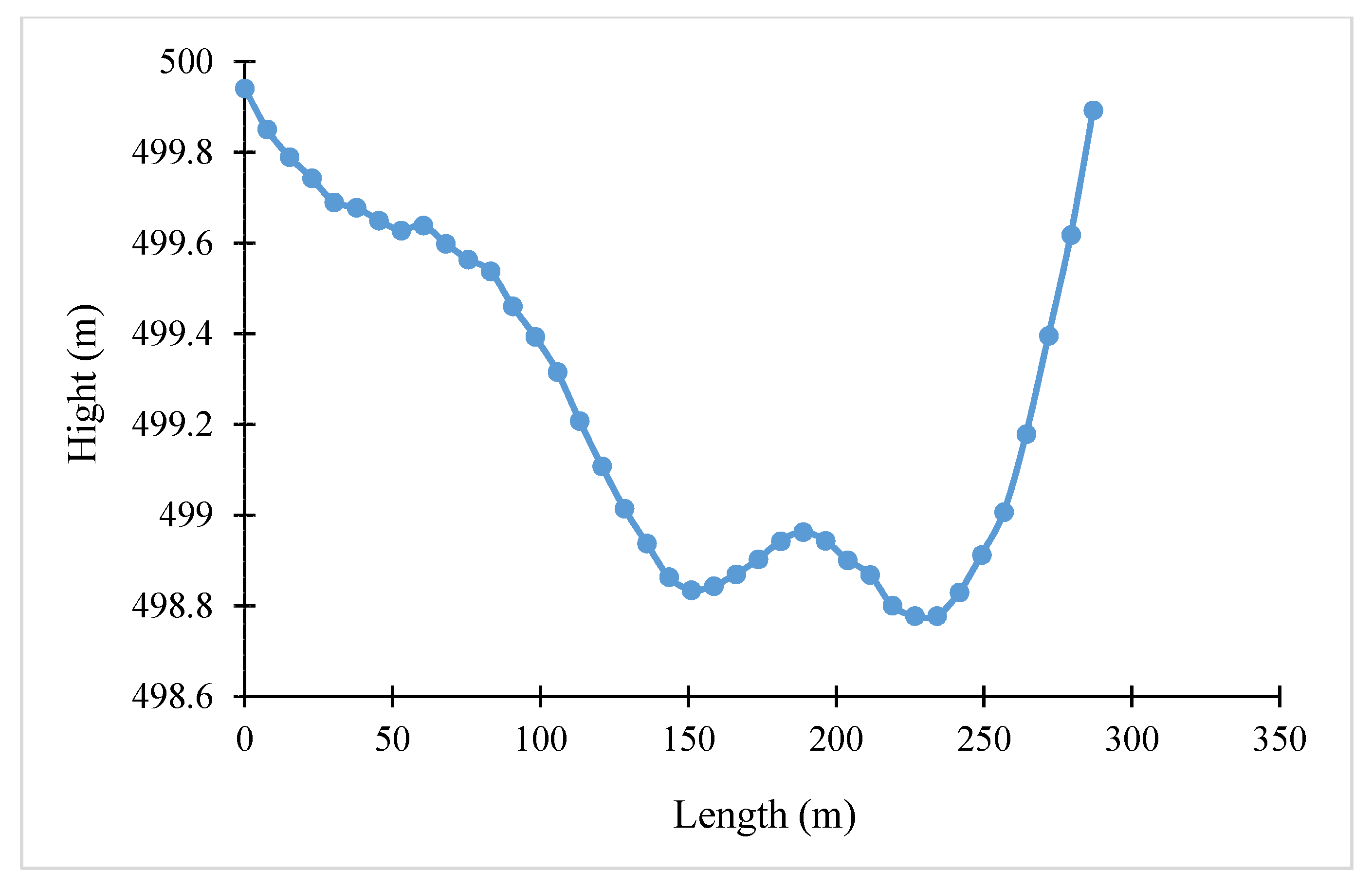
Figure 10.
Example of channel cross-sections extracted from the 10 m DEM for the GSSHA model.

Figure 11.
Comparison between simulated discharges for HEC-HMS and GSSHA models and the observed peak discharge at the outlet of Wadi Al-Nu’man before calibration.
Figure 11.
Comparison between simulated discharges for HEC-HMS and GSSHA models and the observed peak discharge at the outlet of Wadi Al-Nu’man before calibration.

Figure 12.
Comparison between calibrated hydrographs for HEC-HMS and GSSHA models and observed peak discharge at the outlet of Wadi Al-Nu’man.
Figure 12.
Comparison between calibrated hydrographs for HEC-HMS and GSSHA models and observed peak discharge at the outlet of Wadi Al-Nu’man.

Figure 13.
Comparison between simulated hydrographs for HEC-HMS and GSSHA models and observed peak discharge at the outlet of Wadi Al-Nu’man.
Figure 13.
Comparison between simulated hydrographs for HEC-HMS and GSSHA models and observed peak discharge at the outlet of Wadi Al-Nu’man.

Figure 14.
The 13 February 2010 outlet hydrographs simulated by HEC-HMS and GSSHA models at the outlet of the Makkah watershed.
Figure 14.
The 13 February 2010 outlet hydrographs simulated by HEC-HMS and GSSHA models at the outlet of the Makkah watershed.

Figure 15.
The 3 November 2018 outlet hydrographs simulated by HEC-HMS and GSSHA models at the outlet of the Makkah watershed.
Figure 15.
The 3 November 2018 outlet hydrographs simulated by HEC-HMS and GSSHA models at the outlet of the Makkah watershed.

Figure 16.
Spatial distribution of cumulative infiltration depths (m) based on HEC-HMS and GSSHA for the 2010 storm event.
Figure 16.
Spatial distribution of cumulative infiltration depths (m) based on HEC-HMS and GSSHA for the 2010 storm event.

Figure 17.
Distributed surface runoff depth map produced by GSSHA.

Figure 18.
The gridded CN for the ModClark model.

Figure 19.
Comparison between simulated outlet discharge for HEC-HMS and GSSHA models.


Table 1.
Maximum 24-h rainfall (mm) for different return periods for the study area based on LPT III distribution.
Table 1.
Maximum 24-h rainfall (mm) for different return periods for the study area based on LPT III distribution.
| Return Period | 2 | 5 | 10 | 25 | 50 | 100 |
|---|---|---|---|---|---|---|
| Rainfall (mm) | 28 | 48 | 64 | 88 | 107 | 129 |
Table 2.
Comparison between GSSHA and HEC-HMS simulation results.
| Model | Peak Discharge (m3/s) | Runoff Volume (m3) | Error in Peak Discharge (%) | ||||||
|---|---|---|---|---|---|---|---|---|---|
| 13 February 2010 | 3 November 2018 | 13 February 2010 | 3 November 2018 | 13 February 2010 | 3 November 2018 | ||||
| Before Calibration | After Calibration | Validation | Before Calibration | After Calibration | Validation | Before Calibration | After Calibration | Validation | |
| GSSHA | 393.2 | 427.6 | 663.6 | 12,866,921 | 14,311,943.5 | 19,455,825.4 | 8.8 | −0.8 | 0.6 |
| HEC-HMS | 847.9 | 429.5 | 689.8 | 17,150,300 | 8,882,200 | 11,933,600 | 96.7 | 0.3 | 4.5 |
Table 3.
Comparison between GSSHA as a reference and HEC-HMS outputs at selected locations.
| Basin | Model | Peak Discharge (m3) | Runoff Volume (m3) | Differences (%) | |
|---|---|---|---|---|---|
| Peak Discharge | Runoff Volume | ||||
| 80B | HEC-HMS | 8.1 | 78,300 | 78.5 | 92.9 |
| GSSHA | 37.6 | 1,097,316 | |||
| 81B | HEC-HMS | 9.1 | 90,100 | 78 | 90.8 |
| GSSHA | 41.3 | 978,141 | |||
| 127B | HEC-HMS | 23.4 | 335,400 | 59.2 | 77.7 |
| GSSHA | 57.3 | 1,505,590 | |||
| 120B | HEC-HMS | 135.4 | 1,882,000 | 26.9 | 59.5 |
| GSSHA | 185.1 | 4,646,771 | |||
| 122B | HEC-HMS | 131 | 1,907,500 | 41.8 | 63 |
| GSSHA | 225.1 | 5,152,439 | |||
Table 4.
Modeling approach.
| Model | Direct Runoff/Overland Flow Routing | Runoff Volume Computation/Infiltration | Channel Flow Routing |
|---|---|---|---|
| HEC-HMS semi-distributed (SCS-UH) | SCS unit hydrograph | SCS curve number | Muskingum |
| HEC-HMS semi-distributed(C-UH) | Clark unit hydrograph | SCS curve number | Muskingum |
| HEC-HMS ModClark | Clark unit hydrograph | Gridded SCS curve number | Muskingum |
| GSSHA | Two-dimensional diffusive wave routing | Green and Ampt with redistribution (GAR) | One-dimensional diffusive wave |
Table 5.
Comparison between GSSHA and HEC-HMS (semi-distributed and ModClark) models.
| Model Type | Rainfall (m3) | Runoff Volume (m3) | Runoff (%) | Losses (m3) | Losses (%) | Peak Discharge (m3/s) |
|---|---|---|---|---|---|---|
| GSSHA | 94,788,583 | 37,622,799 | 39.7 | 53,142,119 | 56.1 | 858.6 |
| HEC-HMS ModClark | 94,963,200 | 40,485,600 | 42.6 | 54,241,500 | 57.1 | 521.5 |
| HEC-HMS (Semi-distributed using SCS transform method) | 94,894,200 | 39,013,400 | 41.1 | 55,880,800 | 58.9 | 1536.1 |
| HEC-HMS (Semi-distributed using Clark transform method) | 94,894,200 | 39,013,400 | 41.1 | 55,880,800 | 58.9 | 1026.3 |
Publisher’s Note: MDPI stays neutral with regard to jurisdictional claims in published maps and institutional affiliations. |
© 2021 by the authors. Licensee MDPI, Basel, Switzerland. This article is an open access article distributed under the terms and conditions of the Creative Commons Attribution (CC BY) license (https://creativecommons.org/licenses/by/4.0/).
Share and Cite
MDPI and ACS Style
Al-Areeq, A.M.; Al-Zahrani, M.A.; Sharif, H.O. The Performance of Physically Based and Conceptual Hydrologic Models: A Case Study for Makkah Watershed, Saudi Arabia. Water 2021, 13, 1098. https://doi.org/10.3390/w13081098
AMA Style
Al-Areeq AM, Al-Zahrani MA, Sharif HO. The Performance of Physically Based and Conceptual Hydrologic Models: A Case Study for Makkah Watershed, Saudi Arabia. Water. 2021; 13(8):1098. https://doi.org/10.3390/w13081098
Chicago/Turabian StyleAl-Areeq, Ahmed M., Muhammad A. Al-Zahrani, and Hatim O. Sharif. 2021. "The Performance of Physically Based and Conceptual Hydrologic Models: A Case Study for Makkah Watershed, Saudi Arabia" Water 13, no. 8: 1098. https://doi.org/10.3390/w13081098
Note that from the first issue of 2016, this journal uses article numbers instead of page numbers. See further details here.