Selecting Suitable MODFLOW Packages to Model Pond–Groundwater Relations Using a Regional Model

Abstract

In large-scale regional models, used for the management of underground resources, it is quite common to find that relationships between the regional aquifer and small wetlands are not included. These models do not consider this connection because of the small amount of water involved, but they should consider the potential for significant ecological impacts if the groundwater resources in the ecosystems associated with these wetlands are mismanaged. The main objective of this work is to investigate the possibilities offered by MODFLOW LGR-V2 to represent (at small scale) the Santa Olalla pond, located in the Doñana Natural Park (South of Spain), and its relationship with the Almonte-Marismas regional aquifer. As a secondary objective, we propose to investigate the advantages and disadvantages that DRAIN, RIVER and LAKE MODFLOW packages offer within the MODFLOW LGR-V2 discretizations. The drain boundary condition with a coarse discretization implemented through ModelMuse allows the most adequate performance of the groundwater levels in the environment of the pond. However, when using lake boundary condition, the use of the MODFLOW LGR-V2 version is particularly useful. The present work also gives some guidelines to employ these packages with the MODFLOW graphical user’s interface, ModelMuse 4.2.

1. Introduction

Numerical flow modeling for groundwater management purposes is commonly used at the aquifer system scale, extending for thousands of square kilometers, with spatial discretization originating cells of hundreds of meters. For some specific cases, the numerical model needs to include the interaction between important, existing ponds and the aquifer. In these cases, the scale of the management model can be too coarse to appropriately represent the hydrogeological processes affecting the ponds under study. Finite element type models can tackle this problem by refining the grid in the area where the pond is located, while keeping a large discretization for the rest of the grid cells. However, classical finite difference discretization methods such as MODFLOW 2005 [1] do not allow this local refinement without increasing the computational cost of the model. Currently, there are also versions of MODFLOW which support unstructured grids. One of them, released in 2013, is MODFLOW-USG [2], which at the moment is not available under any free graphical user interface. Another version is MODFLOW 6 [3], which was released in 2017. MODFLOW 6 incorporates capabilities as coupling regional-scale groundwater models with multiple local-scale groundwater models, and it is still improving every year, including old packages of MODFLOW 2005. However, its use in the scientific literature is very scarce, probably due to the big changes on its working methodology. Still, nowadays, MODFLOW 2005 versions are a standard use in groundwater modeling. The development of a special MODFLOW version, Local Grid Refinement-2 (LGR-2) [4], permits to perform a “zoom” in a small area around the pond, at the same time that the regional model can be run. There are several different studies using MODFLOW LGR-2. One of them analyzes the performance of different LGR implementations (share points, LGR-1, and ghost points, LGR-2) and then the performance of MODFLOW-LGR with a regional-scale model [5]. Another study completes a sensitivity analysis for groundwater flow in combination with a solute transport model [6]. However, no references have been found to analyze how MODFLOW-LGR can represent the aquifer–pond interchanges.

In addition, different MODFLOW packages have been developed to represent diverse implementations of the Cauchy boundary condition, which can be used to simulate the aquifer–pond interactions. Several studies use the DRAIN package to simulate groundwater in mines [7,8] or to represent surface–groundwater relationships [9,10,11]. The LAKE package [12,13] has also been used to model surface–groundwater exchanges. The last version, LAK7, is derived from LAK3 [14] and can consider more than one lake. Hunt et al. [15] give guidelines on selecting an appropriate grid spacing for lake simulations, but with a fine discretization for the whole model. It is difficult to translate their conclusions with a classical finite different configuration in a large-scale regional groundwater flow model used for management purposes. The work of El Zehairy et al. [16] applied and disclosed the complexity of artificial and natural lake interactions with groundwater. They worked with a transient model in MODFLOW-NWT, applying the LAK7 package within its integration with the STREAMFLOW ROUTING package, SFR7 [17], and the UNSATURATED-ZONE FLOW package, UZF1 [18]. They reached the conclusion that, in contrast to natural lakes, the reservoir interaction with groundwater was primarily dependent on the balance between lake inflow and regulated outflow, while the influences of precipitation and evapotranspiration played secondary roles. This is typical of the artificial nature of the lake. They also probed the water table’s dependence on lake stage, lakebed leakance, groundwater head distribution and hydrogeological system parameterization [16]. Anderson et al. [19] tested with a former version of MODFLOW [20] the use of a high-K method zone to reflect the lake head when it is not known a priori. It consists of assigning high hydraulic conductivity (K) values to nodes which represent a pond. Results demonstrated that the high-K method accurately simulates lake heads, but it has more cumbersome postprocessing and longer run times than using the standard LAKE package in simulations. Another boundary condition which is used to simulate lakes and wetlands is the RIVER package [20]. Jones et al. [21] used both the LAKE and RIVER packages to simulate lakes in Minnesota (USA). They highlighted that, when using the RIVER package to represent closed surface water bodies, care should be taken because of an unrealistic, unlimited water input from the river cells to the aquifer. This also implies that stages in the lakes will not be affected by nearby pumps because these river cells may introduce more water to the model as groundwater extraction increases. Other MODFLOW packages that are used to explain the groundwater–pond connection are the GENERAL HEAD BOUNDARY (GHB) and STREAM (STR) packages [22]. Dusek and Veliskova [23] compared the input options of RIVER and STREAM packages, concluding that differences between the computed groundwater tables were minimal with both packages.

Brunner et al. [24] carried out a comparison between the effects of different vertical and horizontal discretization when using the RIVER MODFLOW package, and they noted some issues and complexities relating to the vertical and horizontal discretizations. However, as far as the authors know, there is no application using the MODFLOW LGR version with different MODFLOW packages to solve the problems related to the discretization of the grid and to represent pond–groundwater interaction. Moreover, there are few studies assessing the impact of the different local refinements on the boundary condition within a coarser model. These evaluations are important to properly simulate the pond–groundwater interchange within a regional model, through adequate grid cell size around the pond.

Doñana Natural Space, located in the southwest of Spain, is one of the largest protected wetlands in Europe [25]. The present study focuses on the case of the Santa Olalla pond, which is the biggest of the natural coastal ponds of Doñana [26]. The Almonte-Marismas aquifer represents a reservoir of groundwater that gives life to the Doñana wetlands and ecosystems [27]. Santa Olalla pond, the only one in the area with a permanent hydroperiod, plays an important role in the conservation of the ecological biodiversity in the zone [28]. This pond is located close to the tourist resort of Matalascañas, which puts this wetland under threat, due to the high water-demand for tourist use and irrigation of crops [29]. This risk worries the Water Management Administration, which have made use of a regional numerical flow model to: (i) understand how the system works, (ii) estimate available resources [30,31] and (iii) evaluate the aquifer contribution, to mitigate the effects of climate change on the pond [32]. This regional groundwater model used coarse grid cells, at a scale that cannot include the presence of local ponds, such as Santa Olalla pond, in the simulation. On the other hand, local models around the Santa Olalla pond have been applied by other authors to estimate the groundwater contribution to the pond and to better understand the functioning of its relationship with the Almonte-Marismas aquifer [33,34].

The present research aims to analyze the possibilities that MODFLOW LGR-2 gives to refine the regional Almonte-Marismas groundwater flow model around Santa Olalla pond. A second objective is the selection of a proper MODFLOW package to represent the pond–aquifer boundary conditions. The resulting model has to suitably simulate the pond–aquifer interaction, as well as being able to be used to estimate groundwater reservoir values for the whole aquifer. These goals were reached by means of (1) changing the discretization of the regional flow model by refining the mesh around the pond, (2) using DRAIN [22], LAKE [14] and RIVER MODFLOW packages [20] to simulate the pond and (3) evaluating their respective performances by means of the simulated piezometry and water balance estimations. The conclusions reached can be extended to any regional model that requires the representation of much smaller scale ponds.

2. Materials and Methods

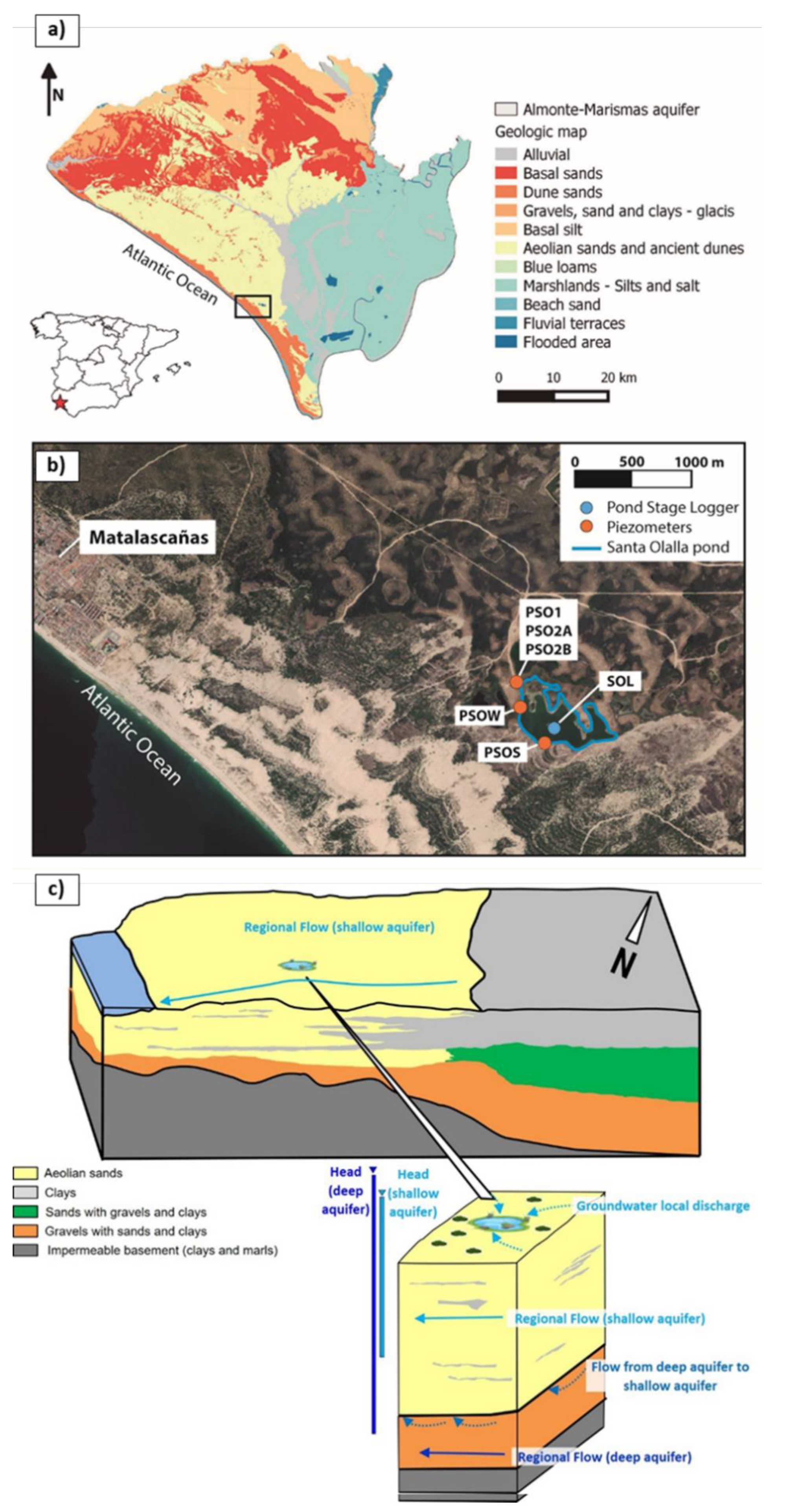
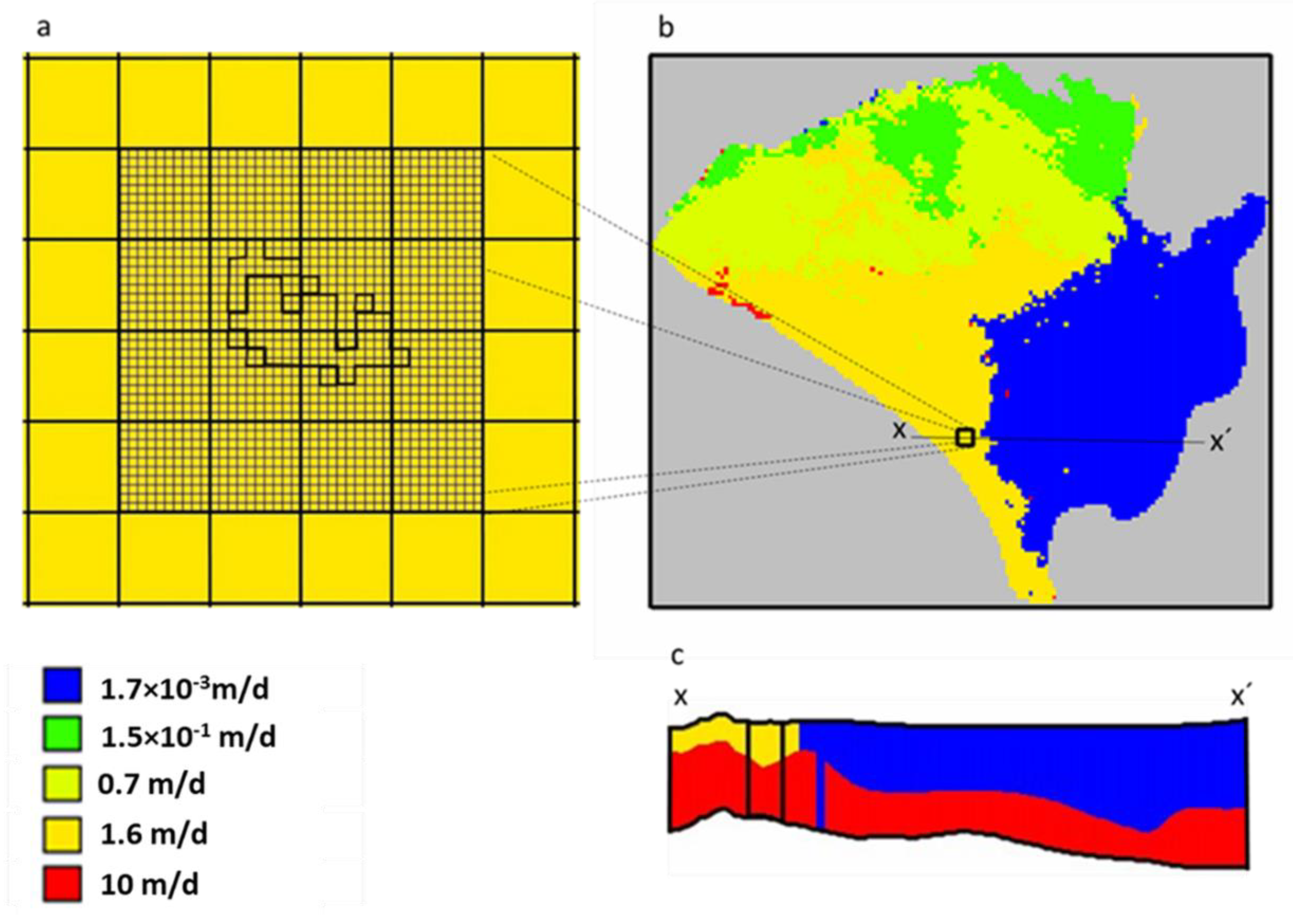
2.1. Study Area

Santa Olalla pond has an approximate area of 0.279 km², while the underlying Almonte-Marismas aquifer system has an area of 2640 km² (Figure 1a). This coast pond is linked to the evolution of the dune buildings located in a large deflation basin of the ancient dune systems. Locally, there is no information on the variability of the parameters of the aquifer and the pond bed. Almonte-Marismas aquifer comprises a free detrital aquifer, where the permeable materials are under the sands and marsh, and semi-confined where they were under the thick detrital materials or confined under materials of low hydraulic conductivity (such as marshland clays) [35]. Groundwater flows from the aquifer to the Santa Olalla pond and, generally, moves from the northeast to the southwest (Figure 1b,c). Nevertheless, it has been verified that, during some extremely dry seasons, Santa Olalla pond changed its direction of flow and started to discharge from the pond to the aquifer along the southern side of the shore [26,33,36]. Doñana has a sub-humid Mediterranean climate with Atlantic influence, it is characterized by regular temperatures, short mild winters, in which temperatures below 0 °C are rarely reached, and dry summers with more extreme temperatures (sometimes exceeding 45 °C). Rainfall is quite variable, and it is characterized by the hyper-annual and interannual variability of rainfall (yearly average 575 mm).

2.2. Data

The use of all the data mentioned below allows to evaluate the pond performance at a local scale. Piezometry around the pond was measured daily by the Spanish Geological Survey (in Spanish: Instituto Geológico y Minero de España, IGME) and the Pablo de Olavide University (POU) during the hydrological year 2016–2017, at five locations: named PSO1, PSO2A, PSO2B, PSOW and PSOS (Figure 1b). The mean annual piezometric heads observed and the characteristics of each of the five piezometers are presented in

Table 1. Characteristics of piezometers. Hydrological year 2016–2017.

Source	Name	X UTM	Y UTM	Average Observed Heads (m)	Max/Min Observed Heads (m)	No. of Measurements	Well Screen Depth (m)	Sensor (Brand)
		(ED50 H30)	(ED50 H30)
IGME	PSO1	190,112	4,098,731	6.33	6.78/5.84	1868	69.5	OTT
								MiniOrpheus
IGME	PSO2A	190,113	4,098,733	6.14	6.60/5.54	2230	27.5	OTT
								MiniOrpheus
IGME	PSO2B	190,113	4,098,733	6.44	6.59/5.75	1217	45	OTT
								Orpheus
POU	PSOW	190,142	4,098,479	6.08	6.48/5.46	2920	15.6	MiniDiver
POU	PSOS	190,374	4,098,113	5.45	5.90/4.95	2920	2.5	MiniDiver

.

Lake stage values were recorded by a Diver water level logger (from the POU), installed in the deepest area of the pond (SOL, Figure 1b). On-site measurements with a staff gauge were used to correct the data. The annual average pond stage in the hydrological year 2016–2017 was 5.25 m a.s.l. Maximum and minimum pond stage measurements for Santa Olalla pond were 5.89 and 4.66 m a.s.l, respectively.

Daily precipitation and temperature data were obtained from the Doñana Biological Station [37]. Evaporation was calculated by applying the modified Penman-Monteith equation [38] and evapotranspiration was computed through the Hargreaves method [39]. The annual average precipitation (P) was 1.22 × 10⁻³ m/d, and the annual average free water evaporation was (EV) 4.56 × 10⁻³ m/d. The flow from the aquifer to the pond was calculated using the mass balance equation:

Q_observed = (P − EV) × A,

(1)

where A is the area of Santa Olalla pond. Applying Equation (1) to the observed annual average aquifer outflow resulted in a value of 0.34 hm³/year, and this value was then used to evaluate the model performance at the local scale. This value is a bit higher than the estimation obtained by Lozano [33], who calculated it to be approximately 0.2 hm³/year, by applying a local mathematical model. A much greater value was estimated in [34], with a 2D segmented-Darcy approach. These authors calculated 1.32 hm³/year of groundwater discharge to the Santa Olalla pond over a seven-month period (between the summer and autumn of 2016). The simplicity of the 2D numerical model, the period of study during the dry season and the underestimation of the aquifer depth (from 2 to 10 m upper layer thickness) could be the reasons for the high aquifer discharge value.

The following objective function (Equation (2)) was used to evaluate the behavior of the different boundary conditions and refinements in the pond environment. By using piezometric heads, lake heads and the interchange flows, the lakebed conductance was calibrated:

O.F. = Σ (Observed head − Simulated head)² + (Observed lake stage − Simulated lake stage)² + (Observed outflow – Simulated outflow)²

(2)

Equation (2) was used to evaluate the adjustment between the calculated and observed piezometric heads in the five available piezometers. In the case of the lake boundary condition, the objective function included the stage measured at the pond. It was not necessary to weight the terms of the outflows because their residuals have the same order of magnitude as the piezometric residuals and the uncertainty of the observations are similar.

2.3. Reference Regional Groundwater Model

The numerical code used to run the regional groundwater model was MODFLOW LGR-2 [4], by means of the free ModelMuse interface [40]. When using MODFLOW LGR without any refining, the execution is equivalent to MODFLOW 2005 [1]. A steady-state simulation was performed, and the regional model was previously calibrated with hydraulic conductivity values. The motivation of using a steady-state model is because it meets with the simplicity required to carry out the objectives of this study (previously mentioned). The steady state represents the average annual situation corresponding to the hydrological year 2016–2017. This average hydrological situation can be accepted for the purposes of the present study.

The model was discretized in two layers, 174 rows and 154 columns, with a grid cell size of 500 × 500 m (Figure 2a). Based on the available geological information, layer 1 is isotropic, while layer 2 is anisotropy with an anisotropy ratio of 0.1 [30]. The upper layer represented the thick sand deposits, occasionally inter-layered with finer sediments (e.g., clays), and the lower layer represented the heterogeneous, lower sand and gravel aquifer. The bottom of this two-layered aquifer system coincides with the top of the underlying Miocene marls (of low hydraulic conductivity) (Figure 1c) [35,41]. Further information about boundary conditions and hydrogeological parameters applied in this regional groundwater model can be found in [32,42]. Constant head in the Atlantic Ocean (Figure 1b) was the main boundary condition affecting the surroundings of Santa Olalla pond. This regional model, in which the relationship of Santa Olalla to the Almonte-Marismas aquifer was not originally included, was used as the reference model in the present work. The results obtained by including the pond with finer discretizations and different MODFLOW packages were compared with this reference model.

2.4. MODFLOW-LGR

The discretization refinement of the model in the area of the Santa Olalla pond was carried out with the Local Grid Refinement MODFLOW version LGR-2 [4], that allowed a higher resolution in a local zone, called a ‘child’. It uses “ghost nodes” situated outside the edge of the child grid and their function is to coordinate the transfer of fluid between the parent and child grids [4,5]. Child models simulate phenomena that need a finer grid than the initial coarse model grid, known as a ‘parent’. The child model covers a subarea of the parent model and can be refined in 2D or 3D.

The regional groundwater model with the coarse mesh and the studied boundary conditions will subsequently be referred to as a ‘parent model’, representing no refinement of the model grid (Figure 2a,b). The red zone in Figure 2 represents the refined area. Grid cells in the pond and its surroundings were subdivided into 10 × 10 horizontal sub-cells (Figure 2c). Two different vertical discretizations were also tested, one of 4 sub-cells and the other of 8 sub-cells in layer 1 (the one that is directly in contact with Santa Olalla pond (Figure 2d,e)).

2.5. MODFLOW Boundary Conditions Representing the Pond

One of the proposals of the present study is to test different MODFLOW packages to represent the aquifer–pond interactions, in both the child and parent models. The first was the DRAIN package [1], which assumes that when the head in the aquifer falls below a fixed drain elevation, there is no flux interchange between the aquifer and the pond. It is a Cauchy-type boundary condition, with the additional constraint that the drain cannot transfer water to the aquifer.

Figure 3a shows the conceptual model of the DRAIN package. The elevation given to the drain is the head of the pond (5.25 m). This boundary condition allows representation of a pond when the pond receives water from the aquifer, as is the case at Santa Olalla in a steady regime. The seepage flux between the pond and the aquifer can be seen as an abstraction of water from the aquifer, at a rate that is proportional to the difference between the head in the aquifer and the fixed drain elevation [1], i.e., the conductivity, C_D, is a parameter imposed by the coefficient of proportionality. The quantification for this flux exchange is expressed by the following equation [22]:

Q_D = C_D × (H_D − h),

(3)

where Q_D is the discharge from the aquifer through the pond (L³/T), C_D is the conductance of the pond bed (L²/T), H_D is the stage of the DRAIN (L) and h is the aquifer head at the pond location (L).

It is important to note that, when working with ModelMuse in 2D or 3D, the conductance value in the drain boundary condition, C_D (see Equation (3) and Figure 3a), can be proportionally computed to the ratio between the area of the polygon, limiting the boundaries of the drain and the area of cell, Ac (Figure 3b). If this option is chosen (i.e., the conductance interpretation is set to be calculated), then the ModelMuse input parameter is considered as conductance per unit area, C_D/A_c (1/T), and the total conductance is equal to this parameter multiplied by the area of the polygon delimitating the drain boundary condition. The parent and child models have different cell sizes and, hence, total conductance in each cell is not the same in both models.

In addition to the DRAIN package, an evapotranspiration boundary condition using the EVT package [22] was added and extended to the peripheral zone of the pond (Figure 3b), where the piezometric head is close to the surface. A computed evapotranspiration rate of 1.18 × 10⁻³ m/d was employed, decreasing this value linearly from the surface to 0.5 m depth. The EVT extension and location were estimated from the difference between the maximum and average flooded Santa Olalla area (Figure 3b).

Another MODFLOW package that was evaluated was the RIVER package [20]. This boundary condition was developed to simulate the surface water/groundwater interaction via the riverbed separating the surface water body from the groundwater system (Figure 4). In the RIVER package, the bottom of the riverbed (H_RBed in Figure 4) and the head in the river (H_R in Figure 4) are necessary parameters. Interchange flux direction depends on the head in the cell connected to the river. If this head drops below the bottom of the riverbed, water enters into the aquifer at a constant rate defined by the gradient between the level of the river and the elevation of the pond bed. When it is above the bottom of the river, water will either leave or enter the aquifer depending on whether the head is above or below the head in the river. The quantification for the flux exchange with this boundary condition is the same as Equation (3), multiplying a conductance term by the difference between the head in the cell and the head in the river. The conductance of the river is defined by Equation (4):

C_R = (K_R × L × W)/M,

(4)

where K_R is the hydraulic conductivity of the riverbed material (L/T), L is the length of reach (L), W is the width of the river (L) and M is the thickness of the riverbed (L).

For Santa Olla pond, the river stage input value (H_R) was set to the average water level measured in the pond (5.25 m a.s.l.). Five different objects were used to represent the river bottom of the pond (Figure 4b) by using bathymetry data taken from [43], ranging from 0.2 to 2.5 m under the ground surface, in the child cells. In the case of the parent river cells, this boundary condition involves 4 cells of the regional model (Figure 4b).

The last boundary condition assessed was the LAKE package [14], which was developed to simulate the effects of surface water bodies, such as lakes and reservoirs, on an aquifer (Figure 5). This boundary condition represents the lake as a volume of space within the model grid, and considers inactive cells extending downward from the upper surface of the grid to the bottom of the deepest layer where the lake is defined [16]. These inactive cells enable the description of the geometry and volume of the lake like a water body out of the aquifer. As a result, it is possible to evaluate the water balance in each time step, and the lake water level that governs for the next computing time interval. The LAKE package considers the lake stage, calculated automatically based on the water budget, which is a function of precipitation, evaporation and natural or anthropogenic inflows and outflows [1]. This condition performs a water balance in the pond, as well as solving the problem of flow in the aquifer system.

In the LAKE package approximation, seepage flux depends on the conductance of the lakebed, C_b, and the conductance of the aquifer, C_a. These parameters define the equivalent conductance, C_e (Figure 5) [14]:

C_b = K_b × A/b = L_b × A,

(5)

C_a = K_a × A/Δl,

(6)

1/C_e = (1/C_b) + (1/C_a),

(7)

C_e = A/((b/K_b) + (Δl/K_a)),

(8)

where A is the cross-sectional area of aquifer section (L²), K_b is the hydraulic conductivity of lakebed material (L/T), K_a is the hydraulic conductivity of aquifer material under the lake in direction Δl (either horizontal or vertical) (L/T), b is the lakebed thickness (L), ∆l is the thickness of the aquifer section (L), which corresponds to half the thickness of the cell below and beside the pond cell, and L_b is the lakebed leakance (1/T). Though this formulation allows to differentiate between vertical and horizonal hydraulic conductivity of the regional aquifer, in the present case, layer 1 is isotropic and K_a has the value in both directions. K_b was also considered to be isotropic.

Figure 5a shows the LAKE package scheme, where P is the precipitation (L/T), p’ is the grill cell center, EV is the evaporation (L/T), h is the water table head (L) and H is the lake surface head (L).

Figure 5b shows the representation of grid cells with the lake boundary conditions of the parent and child models at the Santa Olalla pond vicinity. Maximum and minimum lake stages are inputs for the LAKE package; for Santa Olalla pond, 5.89 and 4.66 m a.s.l were adopted, respectively. These values correspond to the annual mean limnimeter data. In any case, these stage parameters are not used for any computation in MODFLOW, they are only an indication of the results’ consistency. MODFLOW prints out a warning message in the main output file (with the extension .lst) when the computed stage is out of this range, but it does not stop the execution [44]. Consequently, it is important to be cautious when executing the LAKE package and check if the resulting stage has no physical meaning.

Drain and river conductance per unit area (C_D/A and C_R/A) and lakebed leakance, L_b, were adjusted with the trial and error approach. The performance aimed to reproduce the observed piezometric heads, the outflow to the pond and the pond stage in the case of using the LAKE boundary condition. Residuals are defined as the difference between observed and calculated values. The fit criterion was the minimization of the objective function results (Equation (2)).

3. Results and Discussion

3.1. Reference Model Parent

The reference model does not include any boundary condition that represents the Santa Olalla pond and, hence, no outflows from the aquifer to the pond can be obtained. Regional Ka in the area occupied by the pond (Equations (6) and (8)) is introduced in ModelMuse with Kx and Ky values of 1.6 m/d for the first layer and 10 m/d for the second layer (Figure 6). For the observation points (Figure 1b), maximum and minimum residuals’ heads obtained with this reference model were a minimum of −0.5 m and a maximum of −0.2 m. For comparison and analysis purposes, residual groundwater levels are represented for all the observation wells in the evaluation of performance figures with dashed lines for the reference model. Negative values indicate that the observed values are lower than the simulated ones.

Various previous numerical modelling studies have been carried out by other authors on the Santa Olalla pond, at a local scale. Lozano [33] carried out a two-layer MODFLOW model of the area surrounding Santa Olalla pond. For the first layer, they calibrated the hydraulic conductivity values with a value of 0.25 m/d, and for the second layer, 5 m/d, which are lower values than the ones used in the present study. It was noticed that the upper layer K had no significant effects on piezometric values around the pond. However, more importantly, hydraulic conductivity in the deepest layer impacts the piezometric results around the pond. As a result of the adjustment process and calibration which was carried out in the steady-state model, the residuals of the piezometric values obtained in the first layer were between 0 and 1 m [33]. On the other hand, Rodríguez-Rodríguez et al. [34] used the segmented Darcy method [45] to quantitatively estimate the groundwater contributions to the pond using daily piezometric data, achieving a value of hydraulic conductivity of 6.48 m/d. Their simulated local 2D profile model detailed the evolution of groundwater levels and assumed the hydraulic connection of the Santa Olalla pond system with the aeolian mantle coastal aquifer area [34].

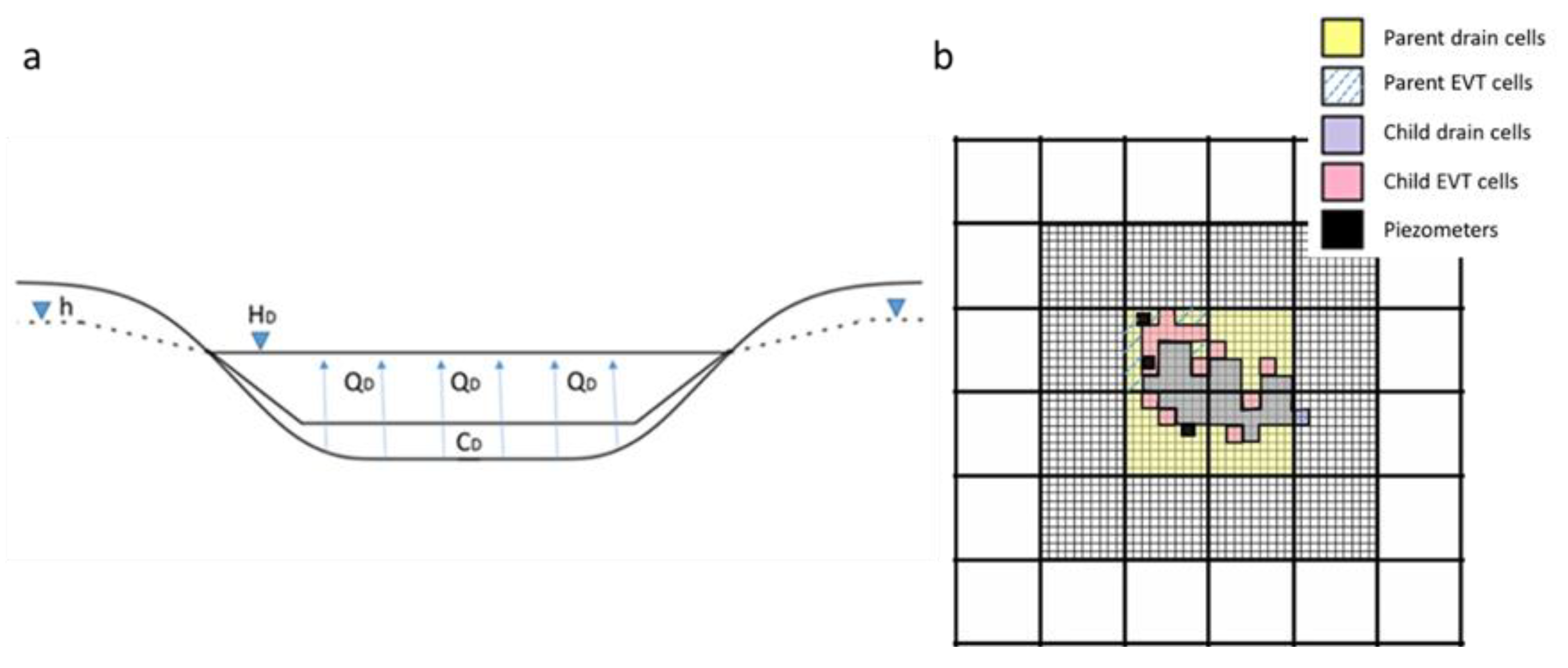
3.2. Parent vs. Child for DRAIN Package

Firstly, the performance evaluation analysis of the piezometric heads to the drain conductance per unit area, C_D/A, was carried out. The parent model residuals are shown in Figure 7a, while the child models results are displayed for both the vertical discretization with 4 layers (Figure 7b) and with 8 layers (Figure 7c).

When comparing residual values with the reference model (Figure 7a), it can be seen that the inclusion of the drain boundary condition in the parent model allowed better performance of the groundwater levels around the pond. In the reference model, PSOS has a residual value close to PSO2A (−0.5 m), and that is why residuals of PSOS cannot be seen in the graph. It can be seen that the evolution of the piezometric head residuals is the same for every discretization (Figure 7); as the value of the C_D/A increases, the absolute values of residuals decrease until zero, and after the residual continues increasing. This is explained by the fact that, when the conductance increases, the aquifer drains more water to the pond, which makes the calculated piezometric heads around the pond decline. Piezometric head residuals have a similar order of magnitude for parent and child models, being, on average, a little smaller in the child models for all piezometers. In other words, child discretization reproduces the observed piezometric heads slightly better than the parent model. For example, the residual average at the different piezometric heads is 0.61 m in the parent model and 0.54 m for the 4- and 8-layer models. Differences between the residual heads of the 4- and 8-layer models are very small (of the order of 10⁻³ m). The vertical discretization of 8 layers (Figure 7c) presents a slightly higher mean residual piezometric head in PSO1 and PSO2A than with the 4-layer discretization (Figure 7b). However, PSOS and PSOW piezometers present smaller residuals in the 8-layer model than in the 4-layer one. The explanation of this feature is attributed to the bigger dispersion of residual piezometric heads within a vertical and horizontal refinement. This can be attributed to the greater horizontal and vertical discretization, where the model can describe the evolution of the piezometric heads in greater detail. That is why the child residuals improve with respect to the parent, and also, where the flow has an important vertical component (proximity of the pond, PSOS and PSOW), increasing the vertical discretization (from 8 to 4) also slightly improves the residuals. When the flow has a preponderant horizontal component, a greater vertical discretization may not contribute and ends up being counter-productive, as in PSO1 and PSO2A.

The performance evaluation analysis of the outflow to the drain conductance per unit area, C_D/A, is illustrated in Figure 8a (parent model), Figure 8b (4-layer child model) and Figure 8c (8-layer child model). As in the case of the piezometric residuals, the range of the residual outflow values do not show relevant differences between parent (0.54 hm³/year) (Figure 8a) and child models (0.44 hm³/year for both the 4- and 8-layer models) (Figure 8b,c). As was expected, when the conductance increased, the flux to the pond was higher. Water balance is influenced by the C_D/A, and as C_D/A increases, the values of the residuals decrease until a C_D/A value is reached, between 2.5 × 10⁻³ and 1 × 10⁻² 1/d, where residuals are 0. For higher values of C_D/A, the values of the residuals begin to increase (Figure 8).

Paying attention to both the performance evaluation analysis (Figure 7 and Figure 8) and the objective function (Equation (2) and

Table 2. Objective function results for the three boundary conditions studied.

CD/A (1/d)	Obj. Function	Drain	Lake	River
0.0001	Parent	0.32	517.74	0.76
	4 Layer	0.42	225.17	0.73
	8 Layer	0.42	64.93	0.73
0.00015	Parent	0.31	229.43	0.73
	4 Layer	0.4	198.21	0.71
	8 Layer	0.4	59.65	0.71
0.00029	Parent	0.28	61.02	0.67
	4 Layer	0.37	88.83	0.65
	8 Layer	0.37	45.64	0.65
0.00119	Parent	0.16	3.77	0.38
	4 Layer	0.21	4.87	0.37
	8 Layer	0.21	5.92	0.37
0.0025	Parent	0.11	1.11	0.17
	4 Layer	0.12	1.22	0.18
	8 Layer	0.12	1.44	0.18
0.01	Parent	0.48	0.45	0.29
	4 Layer	0.28	0.4	0.18
	8 Layer	0.27	0.47	0.18
0.018	Parent	0.87	0.45	0.65
	4 Layer	0.5	3.56	0.37
	8 Layer	0.48	0.34	0.36
0.027	Parent	1.18	0.45	0.95
	4 Layer	0.65	4.12	0.52
	8 Layer	0.63	0.56	0.5

), an optimum value of C_D/A for performing the parent model and the child models is 2.5 × 10⁻³ 1/d.

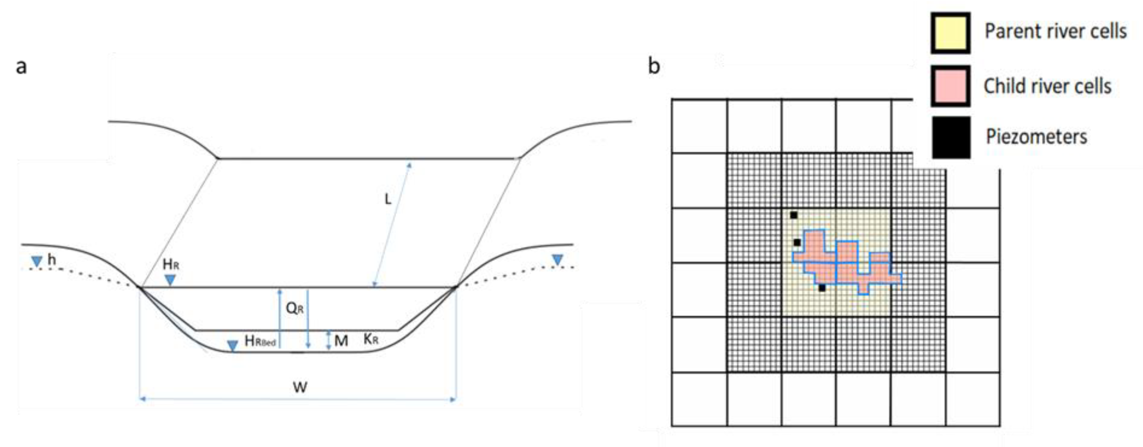
3.3. Parent vs. Child for RIVER Package

Figure 9 shows the performance evaluation analysis of RIVER package for the parent model version (Figure 9a) and child models with 4 and 8 layers (Figure 9b and Figure 9c, respectively). As in the drain case, residuals of the piezometric values show the same evolution in the three performance analyses; as C_R/A increases, the absolute residual values decrease until an optimum value of C_R/A is reached, which makes the residuals close to zero. Then, for higher values of conductance, the simulated piezometric heads are lower than the observed values and absolute residual values begin to increase again (Figure 9).

Residual outflow values (Figure 10) also show the same evolution as the evaluation analysis performed with the drain boundary condition. Residual outflow values of child (4 and 8) layers are practically the same, and differences between child models, with respect to the parent model, get more significant with values of C_R/A being greater than 2.5 × 10⁻³ 1/d. The optimum C_R/A value for the parent would be 2.5 × 10⁻³ 1/d with an objective function value of 0.17 and 2.5 × 10⁻³ or 1 × 10⁻² 1/d in the child models, with an objective function value of 0.18. On the other hand, outflow values do not seem to be unrealistic, and unlimited water input from the river boundary condition cells to the aquifer has been observed by other authors, such as Jones et al. [21].

Brunner et al. [24] presented some consequences of using the RIVER package. They stated that there would be an underestimation of the infiltration flux if there is a disconnection between the groundwater and the surface water. In the present case, the parent and child models tested always had a water table higher than the elevation of the riverbed bottom and, hence, this problem does not appear. At the same time, the use of MODFLOW LGR-V2 allowed us to avoid the errors related to the coarse horizontal and vertical discretization when using the DRAIN or RIVER packages, as reflected by Brunner et al. [24]. The horizontal discretization can cause a discrepancy between river width and cell width, resulting in an error in the water table position under the river. A coarse vertical discretization is often used to avoid the drying out of cells, and this may result in an error in simulating the height of the groundwater dome.

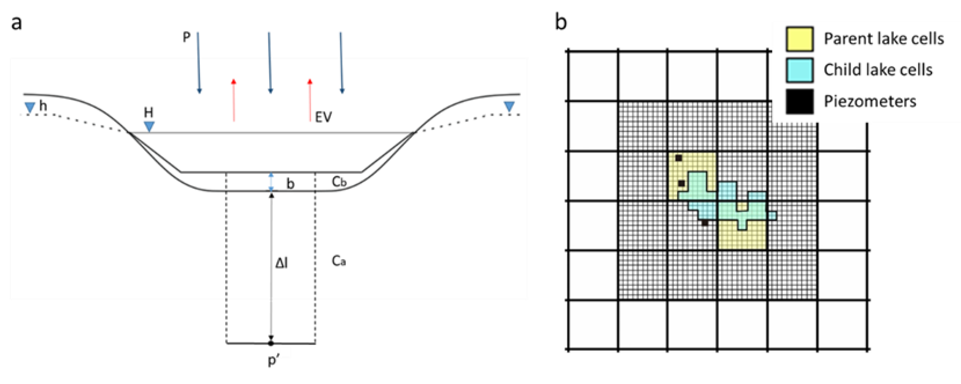
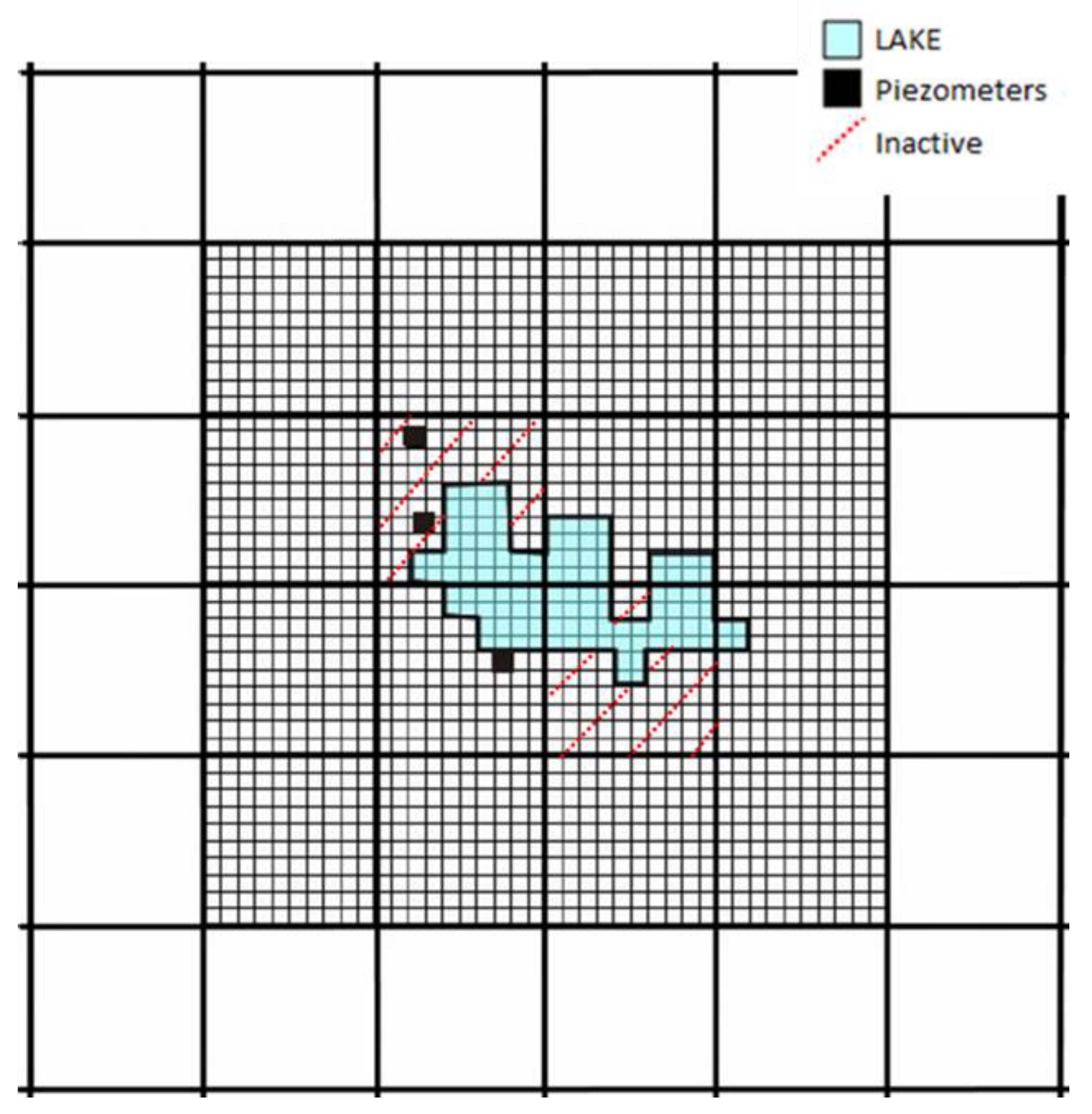
3.4. Parent vs. Child for LAKE Package

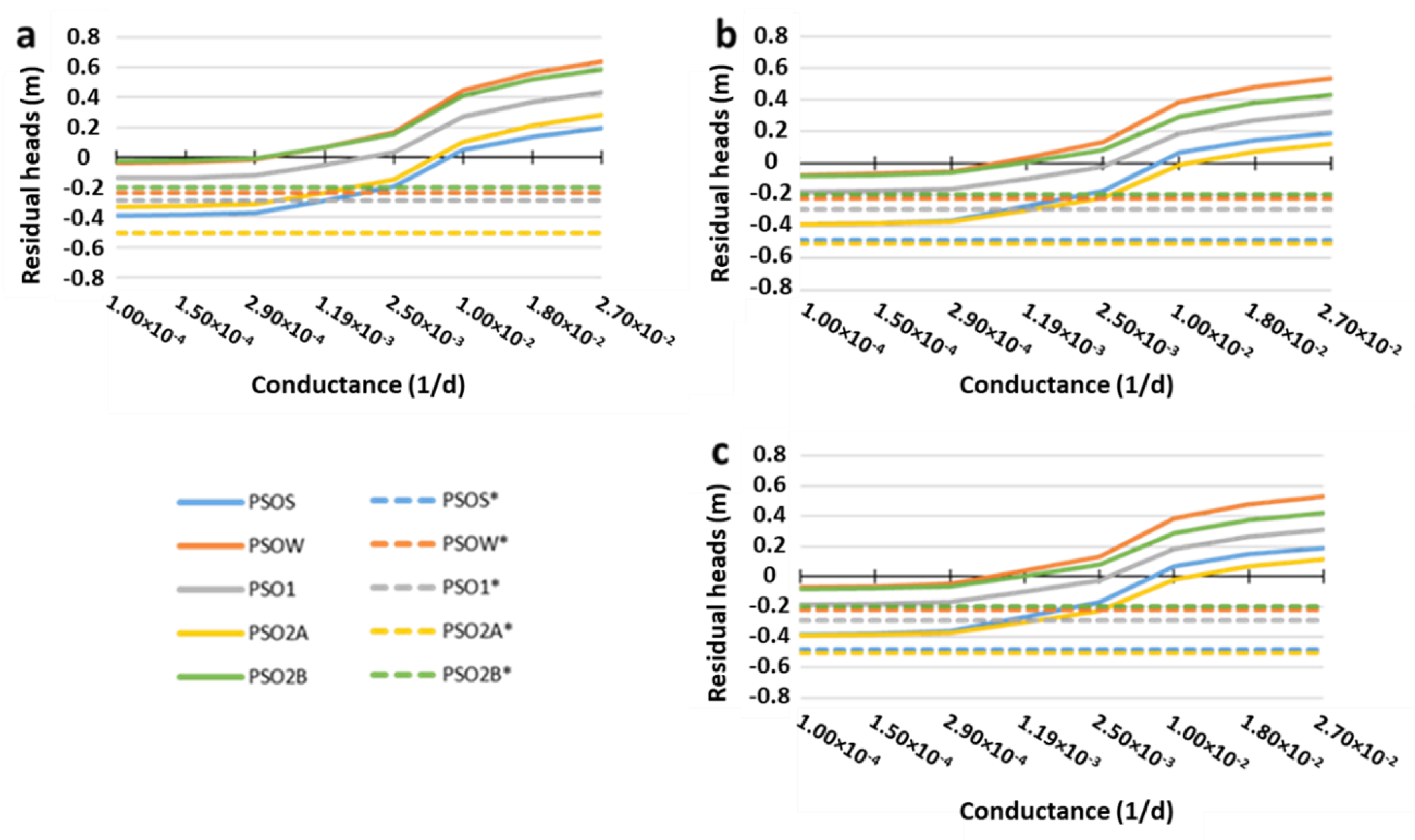
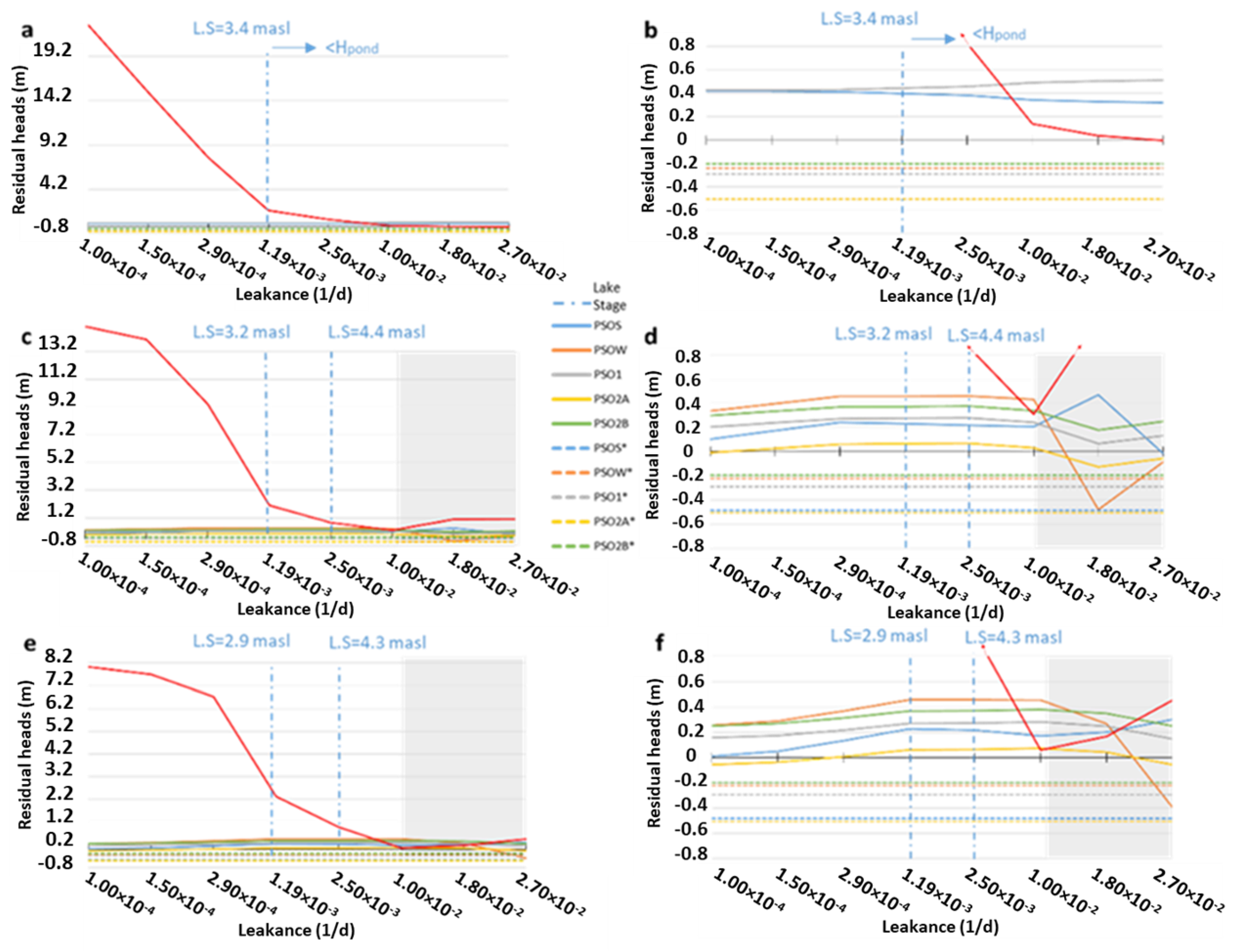
3.4.1. Piezometry Results in the Parent Model (LAKE Package)

The performance evaluation analysis using the lake boundary condition is displayed in Figure 11, showing residuals of piezometric heads in the parent model (Figure 11a,b), child model with a 4-layer vertical discretization (Figure 11c) and child model using 8 layers (Figure 11d). For the parent model, the results should be interpreted bearing in mind that the lake is draining the aquifer from the cells surrounding the area comprising the lake and that the first layer bottom within the pond area ranges from −59.69 to −55.26 m a.s.l, which is much deeper than the maximum real pond bed depth of about −2.5 m a.s.l. In addition, the parent model only computes piezometric heads at two piezometers (PSOS and PSO1). The other three piezometers are in the same cells where the lake is situated, and the LAKE package inactivates these cells (PSOW, PSO2A and PSO2B).

For certain leakance values, it can be observed that the average piezometric residuals decrease, with respect to those obtained in the reference model without the use of the boundary condition (e.g., PSOS in Figure 11a,b). It is difficult to see PSOS in Figure 11a, b, because, in the reference model, the PSOS and PSO2A piezometric results are similar (PSOS* and PSO2A* in Figure 11a,b). For PSOS, the inclusion of the lake boundary condition allows better representation of the local piezometry around the pond. However, for the other piezometer (PSO1), residual values are worse than those obtained in the model without any boundary condition (i.e., reference model PSO1*).

Taking into account the fact that the maximum head of the lake stage is 5.89 m a.s.l, and the head of the pond bed is 3.4 m a.s.l, the most plausible results in the parent model are those whose leakance values are higher than 1.19 × 10⁻³ 1/d.

3.4.2. Piezometry Results in the Child Models (LAKE Package)

Piezometry, lake stage and outflow results showed abnormally high residuals for leakances (L_b) higher than 1 × 10⁻² 1/d in both child models (in Figure 11 and Figure 12, colored grey). This fact could not be explained, and it was attributed to numerical instability problems, being smoother in the 8-layer model (Figure 11d vs. Figure 11f and Figure 12c vs. Figure 12d).

In the child models, the leakance values with physical sense are situated between 1.19 × 10⁻³ and 1.25 × 10⁻³ 1/d (shown with dashed lines in Figure 11a,c,e). Residual piezometric heads are lower in the child models than in the parent model (order of 2 × 10⁻¹ m). For example, a leakance of 1 × 10⁻² 1/d results in parent model residuals of 0.34 m (PSOS) or 0.49 m (PSO1) while, for the 8-layer child model, residuals are 0.17 m (PSOS) or 0.28 m (PSO1). On the other hand, piezometric head residuals are more sensitive to leakance values than in the parent model. The trend of the piezometric heads is similar in both the 4- and 8-layer child models. For these child models, a greater sensitivity to leakance was observed in the PSOS and PSOW piezometers. This could be due to their proximity to the pond.

The low sensitivity of residual piezometric values, when modifying the leakance value, for both parent and child models, contrasts with the results obtained by Jones et al. [21] and may be an indicator that conductance of the regional aquifer, C_a, plays a major role in the equivalent conductance (Equation (6)). This happens because ∆l values are high in the discretizations used and, as the discretization is refined, K_a loses weight in the equivalent conductance, Ce (Equation (8)). Due to this fact, it is important to note the importance of also simulating and evaluating the lake stage to get a realistic leakance value. Similarly, Jones et al. [21] noticed that horizontal hydraulic conductivity values for the aquifer have a large impact on the model’s ability to simulate lake water levels and base flows.

As found by Jones et al. [21], lake water levels are sensitive to lakebed leakance. For high leakance values, the pond level increased and water began to enter from the immediate area of the aquifer, as expected. Then, it was seen that the head of the piezometer close to the pond on the south coast (PSOS) increased (Figure 11b), while the regional piezometric level located at the second layer (PSO1) decreased. However, with low leakance values, the lake stage got high residuals in the parent model but the lake levels were unreal because they were below the lakebed stage.

To understand lake stage residuals behavior, it is important to bear in mind that MODFLOW equals the pond bed to the cell bottom, in which the lake boundary condition is located. Therefore, the code considers the existence of the lagoon while the calculated lake stages are higher than the bottom of the cell, ignoring the input data of maximum and minimum lake stages and the lakebed levels, and continuing recharging water from the pond to the aquifer. Only if the calculated lake stage is equal, or less, to the bottom of the lake cell, there is no flux between the aquifer and the pond. For example, in the case of using a leakance of 1 × 10⁻⁴ 1/d, the residuals of lake stage achieved 22.74 (Figure 11a), 14.99 or 8.04 m (Figure 11b). The solution is to align cell bottoms with the pond bathymetry. However, this approach is not always recommended due to the abrupt variations of discretization that could be produced. This fact was somehow pointed out by Jones et al. [21] when they stated that the model that uses the LAKE package should be applied to simulations of hydrologic features and processes that can be accurately represented in the model area at the scale of the model cells. In any case, the literature consulted regarding the LAKE MODFLOW package does not explicitly prevent this problem. It is in the printed output file where it can be seen that the resulting lake stage has no physical meaning.

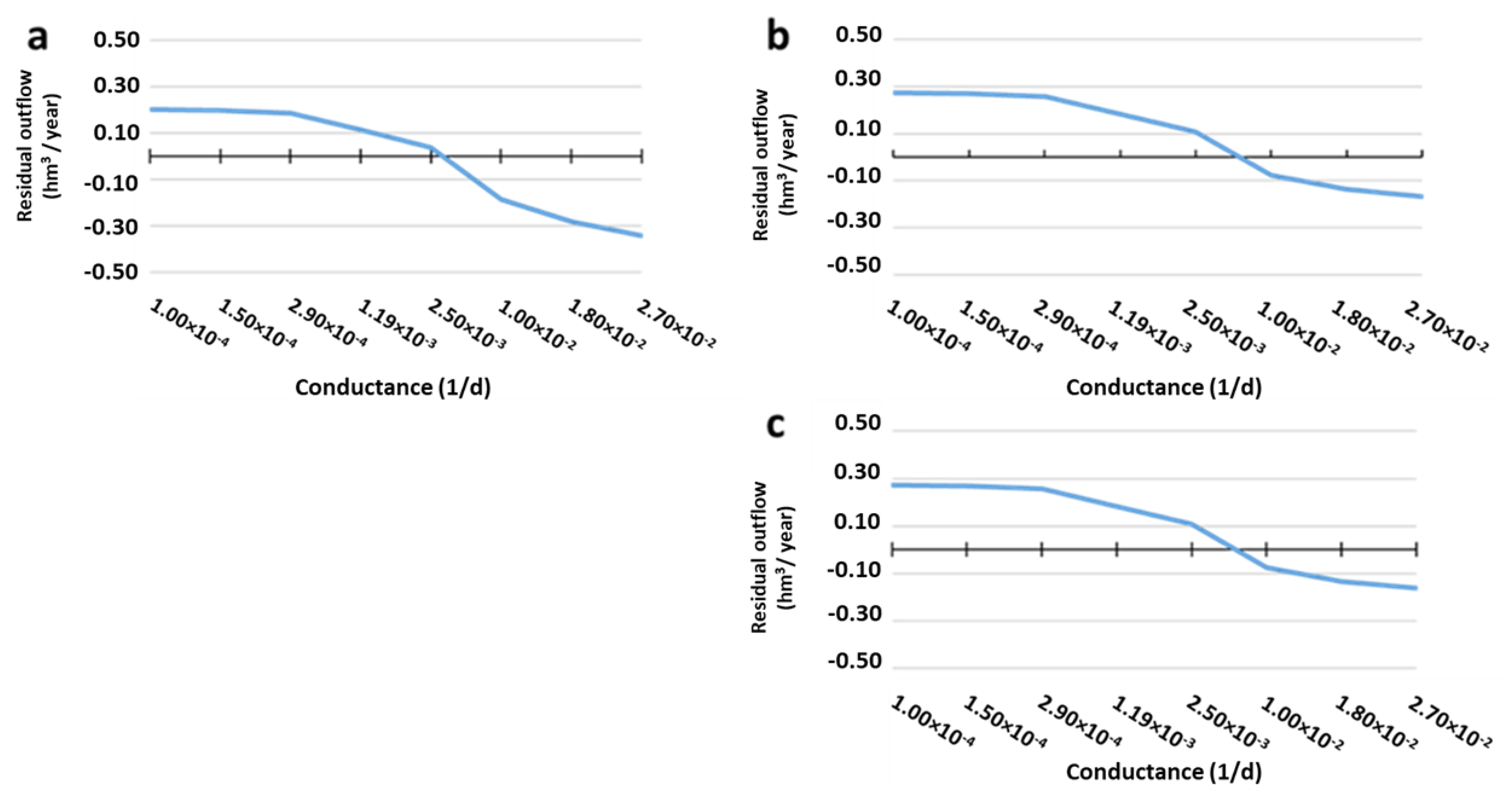
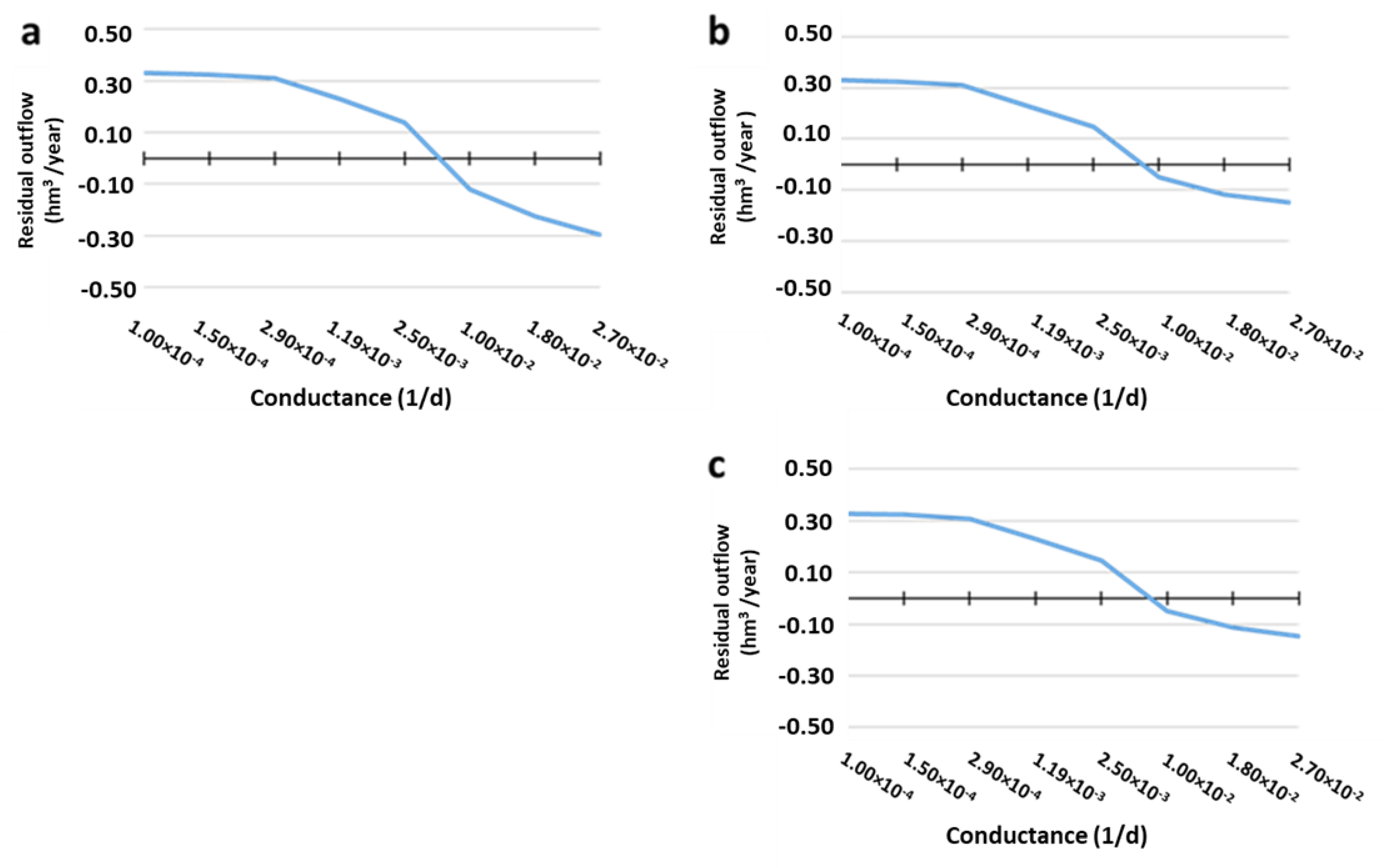
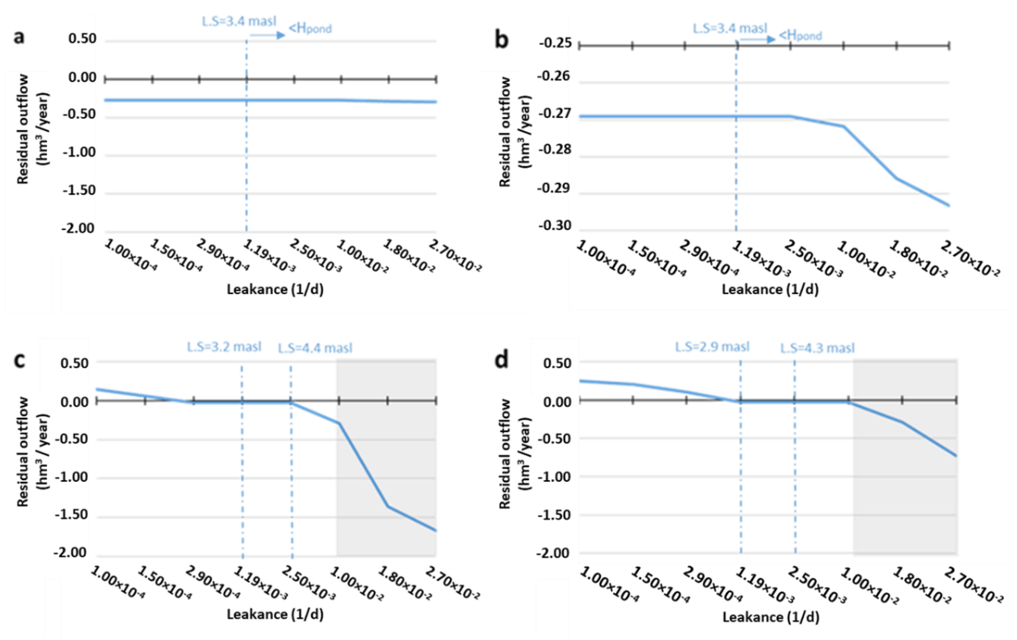
3.4.3. Outflow Results (LAKE Package)

In the parent model, the outflow values from the aquifer to the pond do not present big variations with different leakances (Figure 12a). When observing this evolution on a smaller scale (Figure 12b), it is shown that outflow residuals are constant for leakance values less than 2.5 × 10⁻³ 1/d, and then, the residuals begin to increase. In the parent model, outflow residuals do not get values close to zero for any studied leakance value. Both facts, again, are possibly happening because the water balance is preponderantly affected by the hydraulic conductivity of the regional aquifer K_a, and the ‘great’ value of ∆l. In all the models, the outflow residual trend decreases as leakance gets higher (Figure 12) because as the leakance is greater, the discharge to the pond increases. Child models are more sensitive to leakance than the parent model, giving better possibilities for performance for the outflow residuals than using the parent model (Figure 12). The explanation is related to the higher ∆l values in the parent model, which reduce the influence of K_b for the equivalent conductance, Ce (Equation (8)). Optimal leakance values are higher in the model with a discretization of 8 layers (from 1.19 × 10⁻³ to 1 × 10⁻² 1/d) than for 4 layers (from 2.9 × 10⁻⁴ to 2.5 × 10⁻³ 1/d), and the residuals are lower for 8 layers than for the model with 4 layers.

Taking into account the objective function for the different models using lake boundary condition (Equation (2), Table 2), the optimal leakance values are: 1 × 10⁻² 1/d (parent), 1 × 10⁻² 1/d (4 layers) and 1.8 × 10⁻² 1/d (8 layers), with the lowest objective function.

3.5. Practical Aspects Using ModelMuse

In the Methodology Section, it was highlighted that in ModelMuse, the conductance value in the drain boundary condition, C_D, can be computed proportionally to the area of the polygon, limiting the boundaries of the drain (Figure 3b). If this option is chosen, then the ModelMuse input parameter is considered to be conductance per unit area, C_D/A (1/T), and the total conductance is equal to this parameter multiplied by the area of the polygon delimiting the drain boundary condition, allowing a conductance calculation in each cell based on the intersected area between the object and the cell.

In the case of using the ModelMuse “enclosed” option in the object assigned with the lake boundary condition, the program only considers the grid cells where the object encloses the center of the cell. Hence, in the present study, just two cells are considered as lake boundary condition (Figure 13). This is one reason why it is recommended to use the MODFLOW LGR with a refined horizontal discretization, because these coarse cells in the parent model do not represent the real size of the LAKE and, in the other two cells, there is no lake boundary condition, where in reality, Santa Olalla pond is present (Figure 13).

4. Conclusions

The inclusion of the drain boundary condition with a coarse discretization and assigning the drain conductance proportionally to the area of the pond allows the best performance of the groundwater levels in the environment of the pond. However, the DRAIN package can only be applied in cases where the surface water body receives water from the aquifer (groundwater-dependent pond).

The RIVER package can be useful in case the variation of the parameter H_R is imposed from the observed lake (or pond) stages. However, as H_R is an input, this package should be rejected if measured pond water levels are needed as a calibration criterion. This package can be applied for gaining or losing surficial water bodies.

The use of lake boundary condition with coarse grids is a complex approximation for several reasons: (i) LAKE package inactivates the cell where it is situated, (ii) the inclusion of lake stage data improves the model local performance process, but vertical cell thicknesses must be of the same order of magnitude as the depth of the pond. (iii) Piezometric heads and flows to the lake-aquifer show lower sensitivity to the lakebed leakance and the aquifer conductance. (iv) Due to the LAKE implementation in MODFLOW, the lake stage calculation does not respect the limits imposed by the maximum stage and the lakebed stage. The lake boundary condition is especially recommended when it is necessary to obtain the water balance and the evolution of lake (or pond) stages, which can be adjusted throughout a calibration process. As for the RIVER package, it enables to simulate gaining or losing lakes.

The use of the MODFLOW LGR-V2 version is particularly valuable if the LAKE package is going to be used. Additionally, it is observed that, in general, the use of a finer discretization is beneficial to obtain more sensitivity models and better subsequent performance at the local scale.

These conclusions can be extrapolated to models with analogous ratios between the regional aquifer dimension and pond scale, which are also common in ponds located at endorheic basins and karst ponds. The present work can also serve to provide guidelines to follow in the correct implementation of LGR, DRAIN, RIVER and LAKE MODFLOW packages with ModelMuse.

References

1. Harbaugh, A.W. MODFLOW-2005, The U.S. Geological Survey Modular Ground-Water Model: The Ground-Water Flow Process; Techniques and Methods; U.S. Geological Survey: Reston, VA, USA, 2005.
2. Panday, S.; Langevin, C.D.; Niswonger, R.G.; Ibaraki, M.; Hughes, J.D. MODFLOW–USG Version 1: An Unstructured Grid Version of MODFLOW for Simulating Groundwater Flow and Tightly Coupled Processes Using a Control Volume Finite-Difference Formulation; Techniques and Methods; U.S. Geological Survey: Reston, VA, USA, 2013.
3. Langevin, C.D.; Hughes, J.D.; Banta, E.R.; Niswonger, R.G.; Panday, S.; Provost, A.M. Documentation for the MODFLOW 6 Groundwater Flow Model; Techniques and Methods; U.S. Geological Survey: Reston, VA, USA, 2017.
4. Mehl, S.W.; Hill, M.C. MODFLOW-LGR—Documentation of Ghost Node Local Grid Refinement (LGR2) for Multiple Areas and the Boundary Flow and Head (BFH2) Package; Techniques and Methods; U.S. Geological Survey: Reston, VA, USA, 2013.
5. Vilhelmsen, T.N.; Christensen, S.; Mehl, S.W. Evaluation of MODFLOW-LGR in Connection with a Synthetic Regional-Scale Model. Groundwater 2012, 50, 118–132. [Google Scholar] [CrossRef] [PubMed]
6. Gedeon, M.; Mallants, D. Sensitivity Analysis of a Combined Groundwater Flow and Solute Transport Model Using Local-Grid Refinement: A Case Study. Int. Assoc. Math. Geosci. 2012, 44, 881–899. [Google Scholar] [CrossRef]
7. Kozar, M.D.; McCoy, K.J. Use of MODFLOW Drain package for simultating inter-basin transfer of groundwater in abandoned coal mines. J. Am. Soc. Min. Reclam. 2012, 1, 27–43. [Google Scholar]
8. Peksezer-Sayit, A.; Cankara-Kadioglu, C.; Yazicigil, H. Assessment of Dewatering Requirements and their Anticipated Effects on Groundwater Resources: A Case Study from the Caldag Nickel Mine, Western Turkey. Mine Water Environ. 2015, 34, 122–135. [Google Scholar] [CrossRef]
9. Zaadnoordijk, W.J. Simulating Piecewise-Linear Surface Water and Ground Water Interactions with MODFLOW. Groundwater 2009, 47, 723–726. [Google Scholar] [CrossRef]
10. Yihdego, Y.; Danis, C.; Paffard, A. 3-D numerical groundwater flow simulation for geological discontinuities in the Unkheltseg Basin, Mongolia. Environ. Earth Sci. 2015, 68, 1119–1126. [Google Scholar] [CrossRef]
11. Han, W.S.; Graham, J.P.; Choung, S.; Park, E.; Choi, W.; Kim, Y.S. Local-scale 696 variability in groundwater resources: Cedar Creek Watershed, Wisconsin, USA. J. Hydro-Environ. Res. 2018, 20, 38–51. [Google Scholar] [CrossRef]
12. Cheng, X.; Anderson, M.P. Numerical simulation of ground-water interaction with lakes allowing for fluctuating lake levels. Groundwater 1993, 31, 929–933. [Google Scholar] [CrossRef]
13. Council, G.W. ISimulating lake-groundwater interaction with Modflow. In Proceedings of the 1997 Georgia Water Resources Conference, Athens, GA, USA, 20–22 March 1997. [Google Scholar]
14. Merritt, M.L.; Konikow, L.F. Documentation of a Computer Program to Simulate Lake-Aquifer Interaction Using the MODFLOW Ground-Water Flow Model and the MOC3DSolute-TransportModel; Water—Resources Investigations Report; U.S. Geological Survey: Reston, VA, USA, 2000.
15. Hunt, R.J.; Haitjema, H.M.; Krohelski, J.T.; Feinstein, D.T. Simulating ground water-lake interactions: Approaches and insights. Groundwater 2003, 41, 227–237. [Google Scholar] [CrossRef]
16. El-Zehairy, A.A.; Lubczynski, M.W.; Gurwin, J. Interactions of artificial lakes with groundwater applying an integrated MODFLOW solution. Hydrogeol. J. 2018, 26, 109–132. [Google Scholar] [CrossRef]
17. Niswonger, R.G.; Prudic, D.E. Documentation of the Streamflow-Routing (SFR2) Package to Include Unsaturated Flow Beneath Streams: A Modification to SFR1; Techniques and Methods; U.S. Geological Survey: Reston, VA, USA, 2005.
18. Niswonger, R.G.; Prudic, D.E.; Regan, R.S. Documentation of the Unsaturated-Zone Flow (UZF1) Package for Modeling Unsaturated Flow between the Land Surface and the Water Table with MODFLOW-2005; Techniques and Methods; U.S. Geological Survey: Reston, VA, USA, 2006.
19. Anderson, M.P.; Hunt, R.J.; Krohelski, J.T.; Chung, K. Using High Hydraulic Conductivity Nodes to Simulate Seepage Lakes. Ground Water J. 2002, 40, 117–122. [Google Scholar] [CrossRef]
20. McDonald, M.G.; Harbaugh, A.W. A Modular Three Dimensional Finite-Difference Ground-Water Flow Model; Techniques of Water-Resources Investigations; U.S. Geological Survey: Reston, VA, USA, 1988; Volume 6, p. 586.
21. Jones, P.M.; Roth, J.L.; Trost, J.J.; Christenson, C.A.; Diekoff, A.L.; Erickson, M.L. Simulation and Assessment of Groundwater Flow and Groundwater and Surface-Water Exchanges in Lakes in the Northeast Twin Cities Metropolitan Area, Minnesota, 2003 through 2013. Chapter B of Water Levels and Groundwater and Surface-Water Exchanges in Lakes of the Northeast Twin Cities Metropolitan Area, Minnesota, 2002 through 2015; U.S. Geological Survey: Reston, VA, USA, 2017; ISSN 2328-0328.
22. Harbaugh, A.W.; Banta, E.R.; Hill, M.C.; McDonald, M.G. MODFLOW-2000, the U.S. Geological Survey Modular Ground-Water Model—User Guide to Modularization Concepts and the Ground-Water Flow Process; Open-File Report 00-92; U.S. Geological Survey: Reston, VA, USA, 2000; p. 121.
23. Dusek, P.; Veliskova, Y. Comparison of the MODFLOW modules for the simulation of the river type boundary condition. Int. J. Eng. Inf. Sci. 2017, 12, 3–13. [Google Scholar] [CrossRef]
24. Brunner, P.; Simmons, C.T.; Cook, P.G.; Therrien, R. Modeling surface water-groundwater interaction with MODFLOW: Some considerations. Ground Water J. 2020, 50, 174–180. [Google Scholar] [CrossRef] [Green Version]
25. Green, A.J.; Alcorlo, P.; Peeters, E.T.; Morris, E.P.; Espinar, J.L.; Bravo-Utrera, M.A.; Bustamante, J.; Díaz-Delgado, R.; Koelmans, A.A.; Mateo, R.; et al. Creating a safe operating space for wetlands in a changing climate. Front. Ecol. Environ. 2017, 15, 99–107. [Google Scholar] [CrossRef] [Green Version]
26. Sacks, L.A.; Herman, J.S.; Konikow, L.F.; Vela, A.L. Seasonal dynamics of groundwater-Lake interactions of Doñana National Park, Spain. J. Hydrol. 1992, 136, 123–154. [Google Scholar] [CrossRef]
27. Suso, J.; Llamas, M.R. Influence of groundwater development on the Doñana National Park ecosystems (Spain). J. Hydrol. 1993, 141, 239–269. [Google Scholar] [CrossRef]
28. Serrano, L.; Zunzunegui, M. The relevance of preserving temporary ponds during drought: Hydrological and vegetation changes over a 16-year period in the Doñana National Park (south-west Spain). Aquat. Conserv. Mar. Freshw. Ecosyst. 2008, 18, 261–279. [Google Scholar] [CrossRef]
29. Serrano, L.; Serrano, L. Influence of groundwater exploitation for urban water supply on temporary ponds from the Doñana National Park (SW Spain). J. Environ. Manag. 1996, 46, 229–238. [Google Scholar] [CrossRef]
30. Instituto Geológico y Minero de España (IGME). Modelo Matemático del Acuífero Almonte—Marismas: Actualización y Realización en Visual Modflow 2005. 2005. Available online: https://www.researchgate.net/publication/264229860_Modelo_matematico revisado_del_acuifero Almonte-Marismas aplicación a distintas-hipotesis de gestion (accessed on 21 November 2018).
31. Instituto Geológico y Minero de España (IGME). Proyecto Para la Actualización del Modelo Numérico (Visual Modflow 4.3, Igme 2007) del Sistema Acuífero Almonte-Marismas, Como Apoyo para el Desarrollo de un Modelo de Gestión y Uso Sostenible del Acuífero en el Ámbito de Doñana (Huelva-Sevilla); Instituto Geológico y Minero de España: Madrid, Spain, 2011. [Google Scholar]
32. Guardiola-Albert, C.; Jackson, C.R. Potential impacts of climate change on groundwater supplies to the Doñana wetland, Spain. Wetlands 2011, 31, 907. [Google Scholar] [CrossRef] [Green Version]
33. Lozano, E. Las Aguas Subterráneas en los Cotos de Doñana y su Influencia en las Lagunas. Ph.D. Thesis, Escuela Técnica Superior de Ingenieros de Caminos, Canales y Puertos, Universidad Politécnica de Cataluña, Barcelona, Spain, 2004. [Google Scholar]
34. Rodríguez-Rodríguez, M.; Martos-Rosillo, S.; Fernández-Ayuso, A.; Aguilar, R. Application of a flux model and segmented-Darcy approach to estimate the groundwater discharge to a shallow pond. Case of Santa Olalla pond. Geogaceta 2018, 63, 27–30. [Google Scholar]
35. Salvany, J.M.; Custodio, E. Características litoestratigráficas de los depósitos pliocuaternarios del bajo Guadalquivir en el área de Doñana; implicaciones hidrogeológicas. Rev. Soc. Geol. Esp. 1995, 8, 21–31. [Google Scholar]
36. Fernandez-Ayuso, A.; Aguilera, H.; Guardiola-Albert, C.; Rodriguez-Rodriguez, M.; Heredia, J.; Naranjo-Fernandez, N. Unraveling the Hydrological Behavior of a coastal Pond in Doñana National Park (Southwest Spain). Groundwater 2019, 57, 895–906. [Google Scholar] [CrossRef]
37. Estación Biológica de Doñana. ICTS de la reserva biológica de Doñana. CSIC, Spain. Available online: http://icts.ebd.csic.es/datos-meteorologicos (accessed on 2 June 2018).
38. FAO. Crop Evapotranspiration. In Guidelines for Computing Crop Waater Requirements; Paper 56; Food and Agriculture Organization of the United Nations Irrigation and Drainage: Rome, Italy, 1998. [Google Scholar]
39. Hargreaves, G.H.; Samani, Z.A. Reference crop evapotranspiration from temperature. Appl. Eng. Agric. J. 1985, 1, 96–99. [Google Scholar] [CrossRef]
40. Winston, R.B. ModelMuse—A Graphical User Interface for MODFLOW-2005 and PHAST; Techniques and Methods; U.S. Geological Survey: Reston, VA, USA, 2009.
41. Naranjo-Fernandez, N.; Guardiola-Albert, C.; Montero-Gonzalez, E. Applying 3D Geostatistical Simulation to Improve the Groundwater Management Modelling of Sedimentary Aquifers: The Case of Doñana (Southwest Spain). Water 2019, 11, 39. [Google Scholar] [CrossRef] [Green Version]
42. Guardiola-Albert, C.; García-Bravo, N.; Mediavilla, C.; Martín Machuca, M. Gestión de los recursos hídricos subterráneos en el entorno de Doñana con el apoyo del modelo matemático del acuífero Almonte-Marismas. Boletín Geol. Min. 2009, 120, 361–376. [Google Scholar]
43. Coleto, M.C. Funciones Hidrologicas y Biogeoquimicas de las Formaciones Palustres Hipogénicas de Los Mantos Eólicos de Los Mantos del Abalorio-Doñana (Huelva). Ph.D. Thesis, Universidad Autónoma de Madrid, Facultad de Ciencias, Madrid, Spain, 2003. [Google Scholar]
44. Winston, R.B. ModelMuse Version 4—A Graphical User Interface for MODFLOW 6; Scientific Investigations Report 2019–5036; U.S. Geological Survey: Reston, VA, USA, 2019; p. 10. [CrossRef]
45. Rosemberry, D.O.; Hayashi, M. Wetland Techniques; Anderson, J., Davis, C., Eds.; Springer: Dordrecht, The Netherlands, 2013; Chapter 3; Volume 1, pp. 87–225. [Google Scholar] [CrossRef]
Figure 1. (a,b) Geological map of Doñana aquifer and location of Santa Olalla pond. (b) Location of piezometers (PSO1, PSO2A, PSO2B, PSOW, PSOS, see Table 1) surrounding Santa Olalla pond and pond stage logger (SOL). (c) Conceptual model.
Water 13 01111 g001
Figure 2. (a) Parent model horizontal view, (b) parent model cross-section profile corresponding to the blue line (x-x’) in (a), (c) child model horizontal discretization of red area appearing in (a), (d) child vertical discretization into 4 layers for the blue profile shown in (c) (y-y’), (e) child vertical discretization into 8 layers for the blue line displayed in (c) (y-y’).
Water 13 01111 g002
Figure 3. (a) Conceptual scheme of DRAIN package and (b) cells where piezometers, drain and evapotranspiration boundary conditions were located in the parent and child models.
Water 13 01111 g003
Figure 4. (a) RIVER package scheme, (b) child and parent model cells where the river boundary condition was introduced.
Water 13 01111 g004
Figure 5. (a) LAKE package scheme (modified from Merritt and Konikow [14]), (b) cells where lake boundary condition was introduced in the child and parent models.
Water 13 01111 g005
Figure 6. (a) Regional calibrated hydraulic conductivity in the first layer of the regional model. Santa Olalla pond area, (b) hydraulic conductivity in the whole aquifer and (c) front view of hydraulic conductivity in the aquifer.
Water 13 01111 g006
Figure 7. Performance evaluation analysis of piezometric heads to DRAIN conductance per unit area, CD/A, for (a) parent model, (b) child model with 4 layers and (c) child model with 8 layers. * Piezometric heads (dashed lines) referred to reference values of the regional model.
Water 13 01111 g007
Figure 8. Performance evaluation analysis of outflow from the aquifer to drain conductance per unit area, CD/A, for (a) parent model, (b) child model with 4 layers and (c) child model with 8 layers.
Water 13 01111 g008
Figure 9. Performance evaluation analysis of residual piezometric heads of (a) parent model, (b) child model with 4 layers and (c) child model with 8 layers, with the boundary condition of RIVER. * Piezometric heads (dashed lines) referred to reference values of the regional model.
Water 13 01111 g009
Figure 10. Performance evaluation analysis of residual outflow values of (a) parent model versus (b) child model with 4 and (c) child model with 8 layers with the boundary condition of RIVER.
Water 13 01111 g010
Figure 11. Performance evaluation analysis of residual piezometric heads of (a) parent model, (b) zoom of the parent model, (c) child model with 4 layers, (d) zoom of child model with 4 layers, (e) child model with 8 layers and (f) zoom of child model with 8 layers with the boundary condition of LAKE. Blue vertical dashed lines show specific calibrated leakance ranges. Between these two values, the model computed realistic lake stages, ranging from the lakebed and the maximum observed stage. The values of these realistic lake stages are indicated at the top of the dashed lines. The grey colored area shows abnormal results. * Piezometric heads (dashed lines) referred to reference values of the regional model.
Water 13 01111 g011
Figure 12. Performance evaluation analysis of residual outflow values of (a) parent model, (b) zoom of parent model, (c) child model with 4 layers and (d) child model with 8 layers with the boundary condition of LAKE. Dashed lines show specific calibrated leakance ranges. Between these two values, the model computed realistic lake stages, ranging from the lakebed and the maximum observed stage. The values of these realistic lake stages are indicated at the top of the dashed lines. The grey colored area shows abnormal results.
Water 13 01111 g012
Figure 13. Representation of the inactive cells in the parent model while using the LAKE package.
Water 13 01111 g013