Sensitivity Analysis for Performance Evaluation of a Real Water Distribution System by a Pressure Driven Analysis Approach and Artificial Intelligence Method

Abstract

Proper performance of water distribution networks (WDNs) plays a vital role in customer satisfaction. The aim of this study is to conduct a sensitivity analysis to evaluate the behavior of WDNs analyzed by a pressure-driven analysis (PDA) approach and the classification technique by using an appropriate artificial neural network, namely the Group Method of Data Handling (GMDH). For this purpose, this study is divided into four distinct steps. In the first and second steps, a real network has been analyzed by using a Pressure-Driven Analysis approach (PDA) to obtain the pressure, and α coefficient, the percentage of supplied flow. The analysis has been performed by using three different values of the design peak coefficient k*. In the third step, the Group Method of Data Handling (GMDH) has been applied and several binary models have been constructed. The analysis has been carried out by using input data, including the real topology of the network and the base demand necessary to satisfy requests of users in average conditions and by assuming that the demand in each single one-hour time step depends on a peak coefficient. Finally, the results obtained from the PDA hydraulic analysis and those obtained by using them in the GMDH algorithm have been compared and sensitivity analysis has been carried out. The innovation of the study is to demonstrate that the input parameters adopted in the design are correct. The analysis confirms that the GMDH algorithm gives proper results for this case study and the results are stable also when the value of each k*, characteristic of a different time hour step, varies in an admissible technical range. It was confirmed that the results obtained by using the PDA approach, analyzed by using a GMDH-type neural network, can provide higher performance sufficiency in the evaluation of WDNs.

1. Introduction

Concern regarding urban water distribution networks has led to increasing awareness and demand for evaluating WDNs to increase their performance and customer satisfaction [1]. The variation in demand can differ hourly, daily, weekly, seasonally, and annually [2,3]. Therefore, assessing water network systems and providing appropriate solutions to increase the level and efficiency of public supply services has been one of the most significant challenges in water engineering over many years. Reviewing previous studies shows that urban water demand is more complex than irrigation, commercial, industrial, and energy demands [4]. Raúl Baños et al. investigated the uncertainty of demand and the influence on the models in terms of resilience Indexes for Water Distribution Networks [5]. The capability of the system to provide the requested demand to all users has been investigated by Farmani et al., who also included demand uncertainty in their approach [6]. The analysis of a network in different conditions has been used in the approach to calibrate hydraulics in both demand-driven analysis (DDA) and pressure-driven analysis (PDA)-based models. Tabesh et al. use a genetic algorithm, analyzing different scenarios of lowest, normal, maximum, and fire consumption [7].

Hence, many studies have been conducted and a wide variety of assessment methods in this area have been introduced. Muranho et al. evaluated the technical performance of water distribution networks using EPANET software. They explored new performance assessment tools. Based on their outcomes, they made several recommendations for evaluation WDNs using new analysis tools [8].

Artificial intelligence approaches have been used successfully for modeling and increasing WDN performance in recent years. Many studies show that these approaches are reliable system modeling techniques for the evaluation of WDNs [9,10,11,12,13,14,15,16]. The data for these approaches could be both measurement data and the results obtained by hydraulic models, or the analysis of networks in real conditions. Fiorini et al. investigated almost 100 different scenarios obtained by a PDA analysis of a real urban water distribution network using the artificial intelligence approaches. Their study demonstrates the capability of the GMDH model to describe the network behavior by assuming input parameters used for the design [17]. Oyebode and Ighravwe used several artificial intelligence techniques to propose the best-predicted model of urban water consumption. The results obtained demonstrated the effectiveness of evolutionary computation techniques [18]. Candelieri et al. evaluated urban water distribution networks using Bayesian optimization to learn optimal control schemes. Their results showed that the proposed Bayesian optimization framework provided more accurate answers compared with other frameworks [19].

By reviewing these previous studies, the importance of improving the level of performance of water distribution networks to increase customer satisfaction is clear. Furthermore, it is important to evaluate model stability when input parameters change, as by changing the value of one input parameter the effective variation of the model results in terms of output must be evaluated. In this study, the factor perturbation method of Veltri et al. and Mc Cuen [20,21,22] is incorporated to estimate the model error due to the variability of input parameters.

This study focuses on the real network application of the PDA approach to perform the network analysis and the GMDH algorithm to classify the network results.

As in a real network, the input parameters adopted in the design could be a little different, it is possible that if their values change, a big variation in the Epanet output and the GMDH model results could occur.

A practical procedure consisted of four distinct steps of hydraulic analysis using the PDA approach, peak coefficient modification, GMDH application, and sensitivity analysis is presented. The analysis is carried out on the Spezzano Albanese network, a town in Calabria, a region in Southern Italy. The proposed methodology is applied to demonstrate its high capability in the prediction and evaluation of water distribution networks with the two consecutive analyses including the first by PDA approach and then by the GMDH algorithm that is the novelty of this study.

2. Methodology

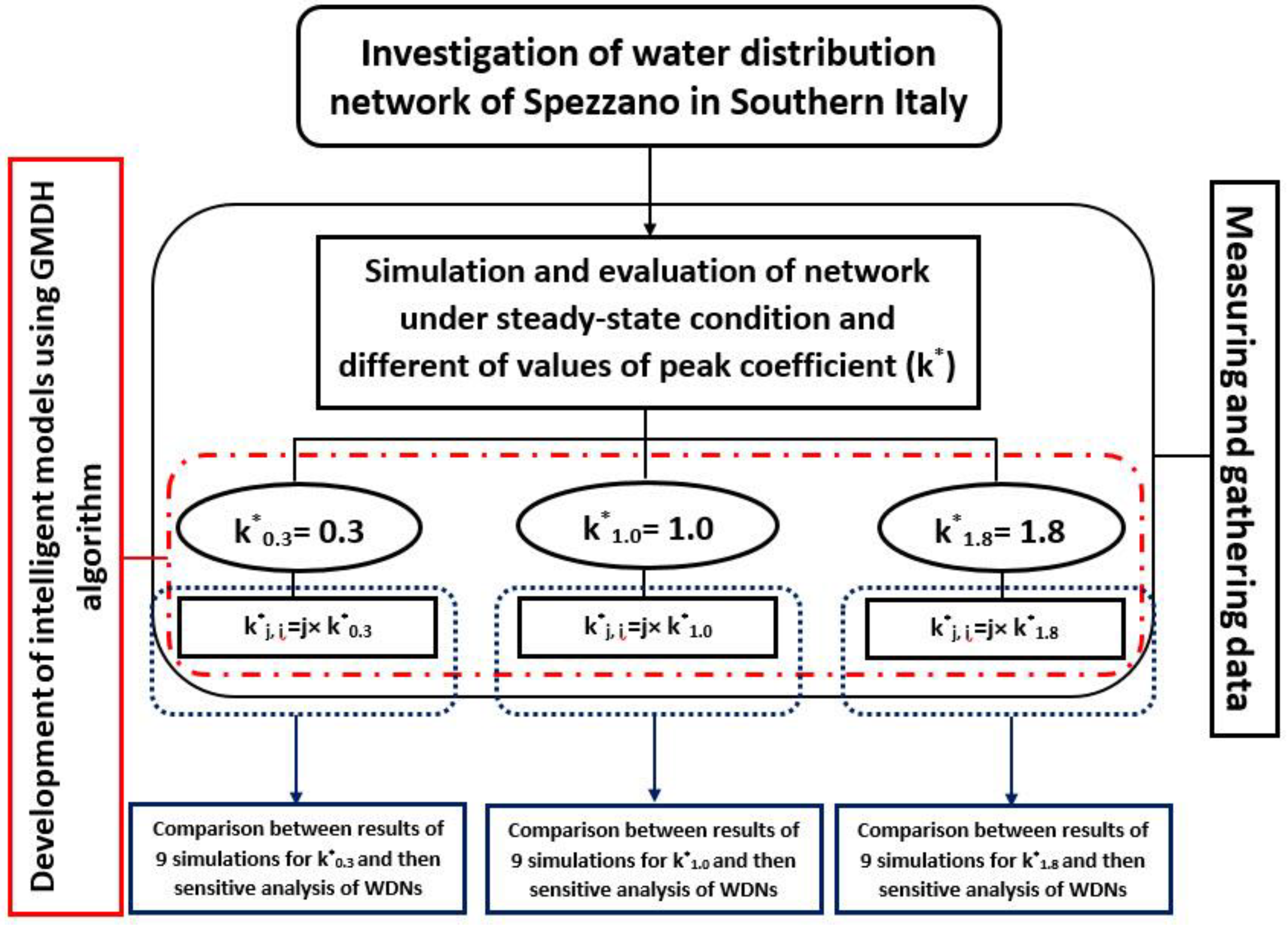
Despite many studies having been conducted in evaluating water distribution networks, more studies are required nowadays according to the importance of the issue and the existence of unknown dynamic factors in WDNs [23,24,25,26,27]. For this purpose, a numerical analysis with the EPANET software and GMDH algorithm as one of the appropriate artificial neural networks has been employed in this study. The flowchart of the study is presented in Figure 1.

An analysis in an extended period has been carried out on the following: the output for each time step has been obtained multiplying the base demand for the corresponding peak coefficient k*. In fact, in a real network, these values are not fixed, and they could change with the user requests. k* values can be obtained by monitoring outflow discharge from each tank, however, there is always a variability of the results for different seasons or depending on climate conditions. Thus, the literature values are assumed for the design. k* values assumed in the analysis are those of a typical pattern proposed for a similar town. Low values characterize night flow and high values, those between 12:00 p.m. and 2:00 p.m. correspond to peak conditions. k* = 1 represents the average condition.

According to Figure 1, the research is based on four steps.

In the first one, the hydraulic parameters of the water distribution network of Spezzano Albanese in Southern Italy including the base demand, pressure, and α (the percentage of real supplied flow) are calculated for three different values of peak coefficient, k*_i. To obtain these values, an iterative procedure by using software Epanet has been adopted. This approach allows defining which nodes work in PDA conditions for each k* value assumed.

The index ‘*’ defines the adopted design values. The i index indicates the assumed values for each analyzed condition of the extended period simulation and it is i = 0.3, 1.0, and 1.8, respectively, for the night (k*_0.3 = 0.3), the average conditions (k*_1.0 = 1.0), and the peak conditions (k*_1.8 = 1.8). In the second step, for each value of k*_i an analysis with a PDA approach has been carried out by varying k*_i in a defined range.

The new values k*_j,i are obtained calculating them as follows in Equation (1):

$${\mathrm{k}}_{\mathrm{j},\mathrm{i}}^{\ast }=\mathrm{j}\times {\mathrm{k}}_{\mathrm{i}}^{*}$$

(1)

The j index is to take into account the variability of k*_i from the design value adopted and it is considered as j = 80%, 85%, 90%, 95%, 100%, 105%, 110%, 115%, and 120%. In this case, the procedure furnishes the number of nodes working in PDA conditions: in these nodes, the user request is partially satisfied.

In the third step, by using all datasets, binary models have been developed to find the best model for evaluating the case study. For this purpose, by changing the control parameters of the algorithm, many models are constructed and developed for finding the best model with maximum accuracy. Finally, in the fourth step, the results are compared and assessed, and sensitivity analysis has been completed. In this step, a sensitivity analysis based on the sensitivity function for train, test, and total is carried out by varying k*_0.3 = 0.3, k*_1.0 = 1.0, and k*_1.8 = 1.8.

As the results change depending on the input values, the aim and innovation of the paper are to demonstrate that the output of the model does not change significantly. The model is stable, and the k* values adopted in the design of the network are correct for management purposes. More details of each step will be presented in the following sections.

2.1. Pressure Driven Analysis (PDA)

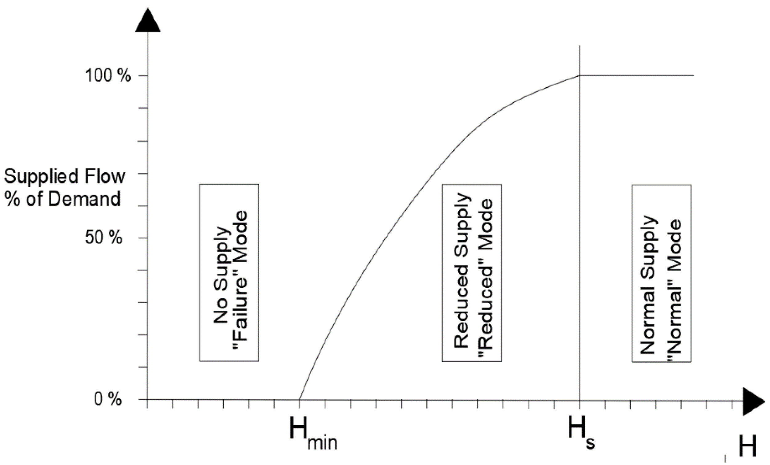
The PDA analysis for a water network is necessary when the head at each node is inadequate to furnish the requested nodal demand Q_BD.

The real delivered demand Q_real for each user depends on the real head value calculated as the totality of elevation (z) and piezometric height (p/γ), i.e., the ratio among pressure (p) and a specific weight (γ). Here H_s, the service head, is defined as the sum of ground level and p/γ_min based on Equation (2):

$${\mathrm{H}}_{\mathrm{s}}=\mathrm{z}+\mathrm{p}/{\mathsf{\gamma }}_{\min }=\mathrm{z}+{\mathrm{H}}_{\mathrm{b}}+{\mathrm{P}}_{\mathrm{ms}}+{\mathrm{P}}_{\mathrm{p}}+{\mathrm{P}}_{\mathrm{D}}$$

(2)

where:

• Z is the elevation of ground level;
• p/γ_min is the lowest piezometric head essential to deliver the demand to the users; it depends on the height of building H_b;
• H_b is the height of each supplied building;
• P_ms represents the minimum pressure essential in each point of the building, usually 5 m;
• P_p indicates the head losses along the riser column;
• P_D represents the head losses between a network node and the base of each building.

Furthermore, H_min is the head necessary to serve users at a ground level based on Equation (3):

H_min = z + P_ms,

(3)

If the head is higher than the service head H_s, Q_real is equal to Q_BD. If the head is lower than H_min there is no service and Q_real = 0. In the other cases, Q_real can be calculated by using Equation (4)

Q_real = α Q_BD,

(4)

The value of α is calculated as the ratio among Q_real and Q_BD: it represents the percentage of supplied flow and it can be obtained using the relations indicated below [28] and according to Figure 2:

$$\mathsf{\alpha }=0\mathrm{if}\mathrm{H}\le {\mathrm{H}}_{\min }$$

(5)

$$\mathsf{\alpha }={\left(\frac{{\mathrm{H}}_{\mathrm{s}}-\mathrm{H}}{{\mathrm{H}}_{\mathrm{s}}{-\mathrm{H}}_{\min }}\right)}^{\frac{1}{\mathsf{\beta }}}{\mathrm{if}\mathrm{H}}_{\min }{<\mathrm{H}<\mathrm{H}}_{\mathrm{s}}$$

(6)

$$\mathsf{\alpha }=1\mathrm{if}\mathrm{H}\ge {\mathrm{H}}_{\mathrm{s}}$$

(7)

where β can be calculated using a calibration model and is related to head loss along pipes. The values of this parameter are between 1.5 and 2 and generally, it is assumed as being equal to 2.

2.2. Sensitivity Analysis

The use of sensitivity analysis allows evaluation of the effect on the calculated results when one of the input parameters changes. The change can reflect a different value estimate either due to an error or a variability under the particular conditions. By changing the value of one input parameter, the effective variation of the model results in terms of output can be evaluated.

The analysis objective evaluates how a model output, depending on n parameters, alters when one of these parameters changes.

There are two approaches to evaluate how the parameter variation influences the overall result: direct differentiation and perturbation by factor method.

By assuming a function F* depending on n parameters (x*₁, …, x*_n), i.e., F* = f(x*₁, …, x*_n), the variation of the function, depending on x_j parameter, can be calculated by direct differentiation as shown in Equation (8):

$${\mathrm{S}}_{\mathrm{xm}}=\frac{\partial {\mathrm{F}}^{*}}{\partial {\mathrm{x}}_{\mathrm{m}}},$$

(8)

By using the factor perturbation method, the input dataset used to obtain model results can be indicated as (x*₁, … x*_m, …, x*_n) and F* = f(x*₁, … x*_m, …, x*_n) is the value of calculated function value obtained by the model. When a single parameter changes a new value of F = f(x*₁, …, x*_m + Δx_m, …, x*_n) can be calculated: the parameter variation can be expressed as Δx_m/x*_m = (x_m − x*_m)/x*_m.

The function ${\mathrm{S}}_{\mathrm{xj}}$, expressing the variation of F* when x*_m changes, can be calculated through the finite differences method according to Equation (9):

$${\mathrm{S}}_{\mathrm{xm}}=\frac{\mathsf{\Delta }\mathrm{F}}{{\mathsf{\Delta }\mathrm{x}}_{\mathrm{m}}}=\frac{{\mathrm{F}(\mathrm{x}}_1^{*},\dots {,\mathrm{x}}_{\mathrm{m}}^{*}{+\mathsf{\Delta }\mathrm{x}}_{\mathrm{m}}^{*},\dots {\mathrm{x}}_{\mathrm{n}}^{*})-{\mathrm{F}}^{*}{(\mathrm{x}}_1^{*},\dots {,\mathrm{x}}_{\mathrm{m}}^{*},\dots {\mathrm{x}}_{\mathrm{n}}^{*})}{{\mathsf{\Delta }\mathrm{x}}_{\mathrm{m}}},$$

(9)

The value of the sensitivity function is S = (F − F*)/F*. Low S values indicate that the model output changes slightly when an input parameter changes: the solution is stable, and it is not sensitive to input data variation.

S can be represented as a function of (x_j − x_j*)/x_j* which is the variation of the parameter x_j* as a percentage of the estimate value x_j* adopted to evaluate F*.

2.3. Group Method of Data Handling Algorithm

In recent decades, artificial intelligence has been developed to overcome both complex and uncertain problems [29,30,31,32,33,34,35]. In recent decades, extensive studies have been conducted on the application of artificial intelligence in various industry sectors and applied sciences [36,37,38,39,40,41,42,43,44]. The Group Method of Data Handling (GMDH) type of neural network is one of the artificial intelligence approaches that are appropriate for dealing with complex systems and was first proposed by Ivakhnenko [45,46,47]. A GMDH-type neural network is one of the machine learning techniques that can be very useful for mathematical modeling, including classification and mapping between input and output vectors. This technique is a linear regression that not only uses the development of modeling but also applies a natural selection such as that in evolutionary algorithms that is unlike other regression methods. Furthermore, a GMDH-type neural network is a type of self-organizing network. Polynomial Neural Network, or PNN, is one of the basic algorithms used to build GMDH models [48,49]. The input data enter the first layer of GMDH and the output of this layer is considered as input data for the second layer and this process continues. If the results of layer (n + 1) are better than the results of layer (n), the algorithm has reached convergence and the optimization process stops. Equation (10) shows a relationship between the approximate function of $\stackrel{\wedge }{\mathrm{f}}$ with output $\stackrel{\wedge }{\mathrm{y}}$ and output y with the least possible error [50,51].

$$\begin{array}{l}\stackrel{\wedge }{\mathrm{y}}=\stackrel{\wedge }{\mathrm{f}}({\mathrm{x}}_{\mathrm{i}1},{\mathrm{x}}_{\mathrm{i}2},{\mathrm{x}}_{\mathrm{i}3},\dots \dots \dots {\mathrm{x}}_{\mathrm{im}})\\ \mathrm{i}=(1,2,3,\dots \dots \dots ,\mathrm{n})\end{array},$$

(10)

The general formula of the GMDH basic neural network is that of Equation (11) [52].

$$\mathrm{y}=\mathrm{a}+{\displaystyle \sum _{\mathrm{i}=1}^{\mathrm{m}}{\mathrm{b}}_{\mathrm{i}}}{\mathrm{x}}_{\mathrm{i}}+{\displaystyle \sum _{\mathrm{i}=1}^{\mathrm{m}}{\displaystyle \sum _{\mathrm{j}=1}^{\mathrm{m}}{\mathrm{c}}_{\mathrm{ij}}}{\mathrm{x}}_{\mathrm{i}}{\mathrm{x}}_{\mathrm{j}}+}{\displaystyle \sum _{\mathrm{i}=1}^{\mathrm{m}}{\displaystyle \sum _{\mathrm{j}=1}^{\mathrm{m}}{\displaystyle \sum _{\mathrm{k}=1}^{\mathrm{m}}{\mathrm{d}}_{\mathrm{ijk}}}{\mathrm{x}}_{\mathrm{i}}{\mathrm{x}}_{\mathrm{j}}{\mathrm{x}}_{\mathrm{k}}+}}{\displaystyle \sum _{\mathrm{i}=1}^{\mathrm{m}}{\displaystyle \sum _{\mathrm{j}=1}^{\mathrm{m}}{\displaystyle \sum _{\mathrm{k}=1}^{\mathrm{m}}{\displaystyle \sum _{\mathrm{l}=1}^{\mathrm{m}}{\mathrm{e}}_{\mathrm{ijkl}}}{\mathrm{x}}_{\mathrm{i}}{\mathrm{x}}_{\mathrm{j}}{\mathrm{x}}_{\mathrm{k}}{\mathrm{x}}_{\mathrm{l}},\dots \dots \dots }}},$$

(11)

Equation (11) works based on input and output data, hence y represents output, and m is considered the number of data for values of x1, x2, x3, …, xm. Generally, the second-order and quadratic form of this polynomial is considered based on Equation (12) [53].

$$\stackrel{\wedge }{\mathrm{y}}=\mathrm{G}{(\mathrm{x}}_{\mathrm{i}},{\mathrm{x}}_{\mathrm{j}})={\mathrm{a}}_0+{\mathrm{a}}_1{\mathrm{x}}_{\mathrm{i}}+{\mathrm{a}}_2{\mathrm{x}}_{\mathrm{j}}+{\mathrm{a}}_3{\mathrm{x}}_{\mathrm{i}}^2+{\mathrm{a}}_4{\mathrm{x}}_{\mathrm{j}}^2+{\mathrm{a}}_5{\mathrm{x}}_{\mathrm{i}}{\mathrm{x}}_{\mathrm{j}},$$

(12)

where ${\mathrm{a}}_{\mathrm{i}}$ are the unknown coefficients and are calculated based on regression techniques. It means that, for determining the total error (E), the difference between the actual output (y) and predicted output $\left(\stackrel{\wedge }{\mathrm{y}}\right)$ should be minimized for each pair of input variables ${\mathrm{x}}_{\mathrm{i}}$ and ${\mathrm{x}}_{\mathrm{j}}$ according to Equation (13) [53].

$$\mathrm{E}=\frac{{\displaystyle {\sum }_{\mathrm{i}=1}^{\mathrm{M}}{{(\mathrm{y}}_{\mathrm{i}}-{\mathrm{G}}_{\mathrm{i}}{(\mathrm{x}}_{\mathrm{i}}{,\mathrm{x}}_{\mathrm{j}}\left)\right)}^2}}{\mathrm{M}}\to \min ,$$

(13)

3. Case Study

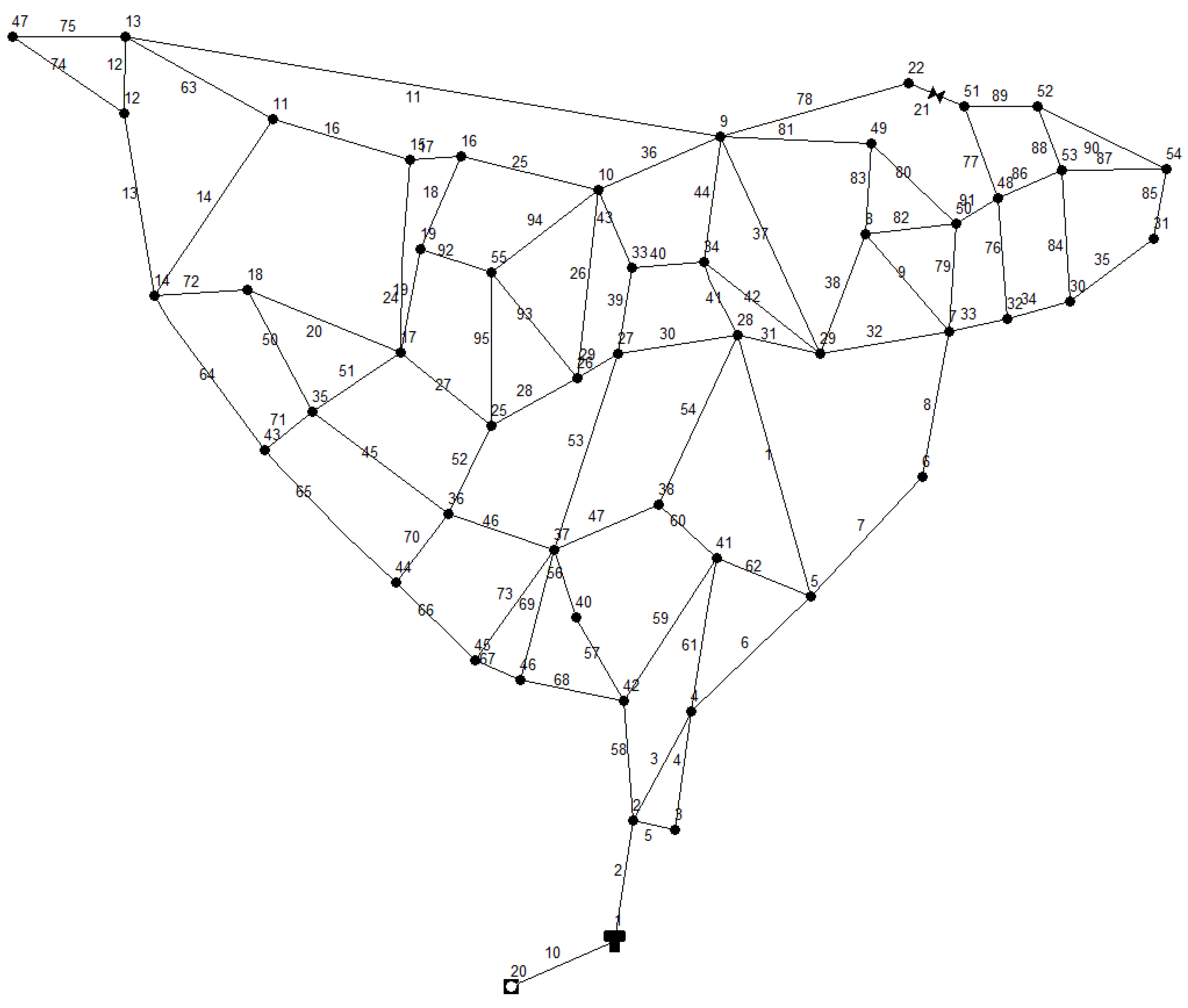
The methodology has been used on a real case related to the water distribution network of Spezzano Albanese (CS, Italy), a little town in the northern zone of Calabria. The network, involving 88 pipes, 49 nodes, and 1 tank, is shown in Figure 3. The total base demand circulating Q_m in the network in steady-state conditions is 29.00 L/s for about 8500 users, according to the real data acquired. The value of H_min varies from 300 to 353 m and H_s varies from about 315 to 368 m. In the analysis, the value of p/γ_min = 20 m has been assumed for each node. These input data are related to winter conditions because during the summer Q can vary significantly with the seasonal fluctuant.

The water distribution system includes a total length of 13,500 m and the pipe diameters differ in the range of 60–200 mm. The tank volume is 200 m³.

In an analysis of a network in an extended period, k*_i is the peak coefficient, which is the ratio between the real demand Q_real in each single one-hour time step and the base demand Q_m.

The chosen values of k*_i coefficient adopted in the analysis are shown in

Table 1. k*_i values and corresponding Q_real.

Scenario	Qreal (L/s)
k*0.3 = 0.3	9.7
k*1.0 = 1.0	29.0
k*1.8 = 1.8	52.2

and they are those of a typical pattern (Figure 4) proposed for a similar town: k*_0.3 = 0.3 describes night condition, k*_1.0 = 1.0 is characteristic of the average conditions and k*_1.8 = 1.8 is the peak condition.

Applying a GMDH approach, three functions, F*_i-Train, F*_i-Test, and F*_i-Total can be calculated and their values for each value of k*_i can be obtained.

To investigate the sensitivity of the model, nine simulations using the k*_j,i value have been conducted for each scenario. Values of k*_j,i are shown in

Table 2. k*_j,i values assumed in each scenario.

j (%)	k*j,i = j × k*i	k*j,0.30	k*j,1.0	k*j,1.8
80%	k*0.8,i	0.240	0.800	1.440
85%	k*0.85,i	0.255	0.850	1.530
90%	k*0.9,i	0.270	0.900	1.620
95%	k*0.95,i	0.285	0.950	1.710
100%	k*1,i	0.300	1.000	1.800
105%	k*1.05,i	0.315	1.050	1.890
110%	k*1.1,i	0.330	1.100	1.980
115%	k*1.15,i	0.345	1.150	2.070
120%	k*1.2,i	0.360	1.200	2.160

:

Hence, 27 simulations, nine for each k*_j,i value were conducted, and then the hydraulic parameters in the network including the base demand, the pressure, and alpha were measured.

By analyzing these data using the GMDH algorithm, the aim is to obtain a good performance of the model. By changing k*_i values according to sensitivity analysis, the aim of the study is to evaluate if corresponding calculated GMDH results are good and stable and very similar to the ones obtained with the design adopted k*_i values.

4. Modelling by GMDH

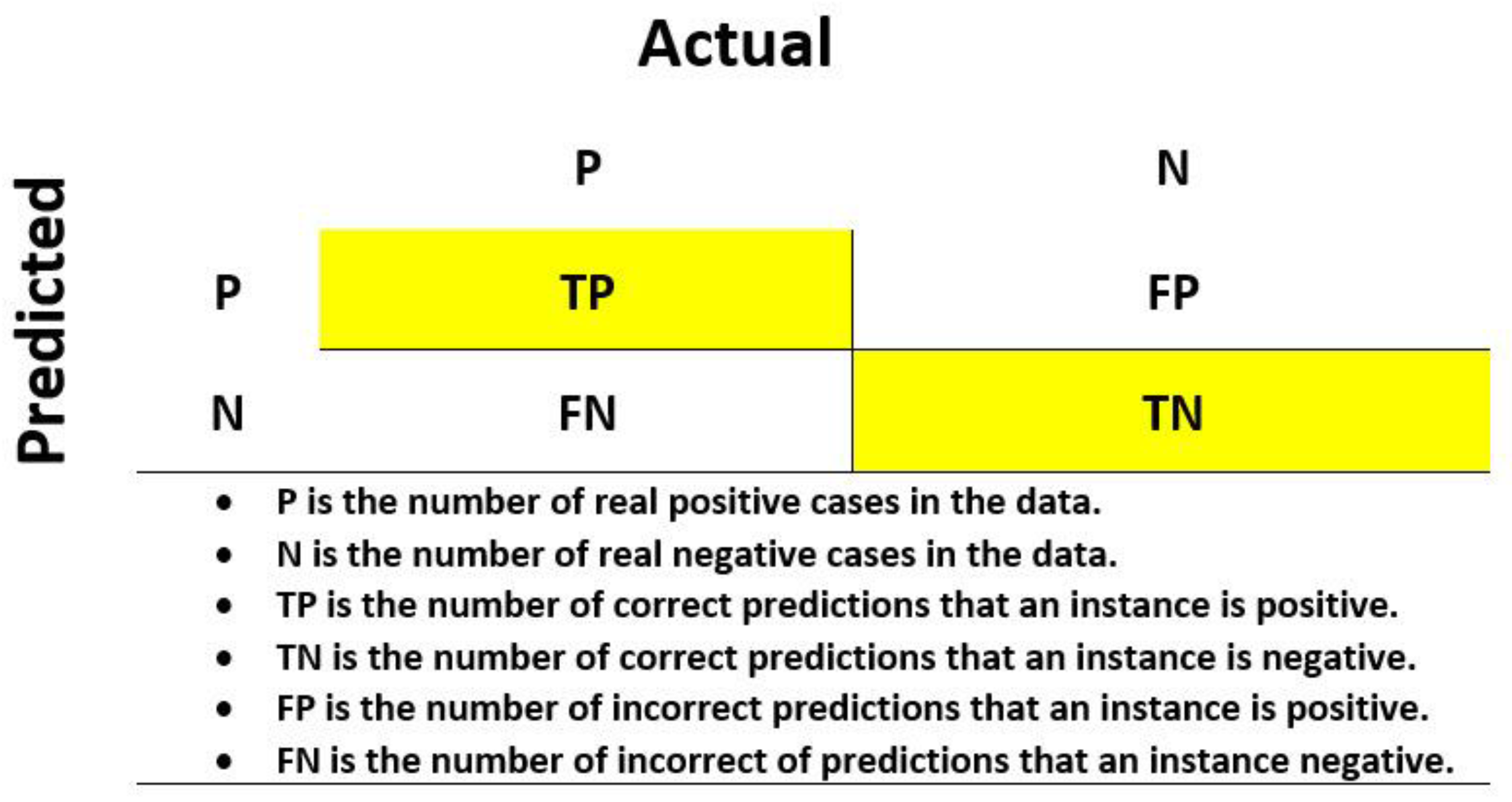
In the first step of the study, the calculated hydraulic parameters after evaluating WDNs by a PDA approach were modeled by the GMDH algorithm. To evaluate and ensure modeling performance, the results of each model were checked with the confusion matrix, which is one of the best performance indexes to evaluate a binary classification. The basic form of a confusion matrix and its relationships (Accuracy and Error) are shown in Figure 5 and Equations (14) and (15) [53,54].

$$\mathrm{Accuracy}=\frac{\mathrm{TP}+\mathrm{TN}}{\mathrm{TP}+\mathrm{FP}+\mathrm{TN}+\mathrm{FN}},$$

(14)

$$\mathrm{Error}=\frac{\mathrm{FP}+\mathrm{FN}}{\mathrm{TP}+\mathrm{FP}+\mathrm{TN}+\mathrm{FN}}=1-\mathrm{Accuracy},$$

(15)

In each modeling, 75% of the dataset (37 data) is considered as a training dataset and the remaining 25% (12 data) is used as the testing dataset [55,56,57,58]. In addition, to obtain the best model, the control parameters of the GMDH must be determined in the best possible way. The Selection Pressure (SP), Maximum Number of Layers (MNL), and Maximum Number of Neurons in a Layer (MNNL) are the control parameters that are determined by suggestions of experts and trial and error methods. The dimensionless parameter SP was considered equal to 0.6 as suggested by some studies and it has a significant effect on the sensitivity of modeling error [59,60]. It is worth mentioning that the two classes (labels) are assigned and considered for the dataset (all nodes), hence labels “0” and “1” are considered for nodes with H < H_s and H ≥ Hs, respectively. In each scenario, several binary classification models are developed and the best models for each scenario are selected. Figure 6, Figure 7 and Figure 8 indicate the results for k*_0.30 = 0.3, k*_1.0 = 1, and k*_1.8 = 1.8, respectively. It is worth mentioning that the accuracy of each class for output and target is shown in the extra columns and rows in the confusion matrices.

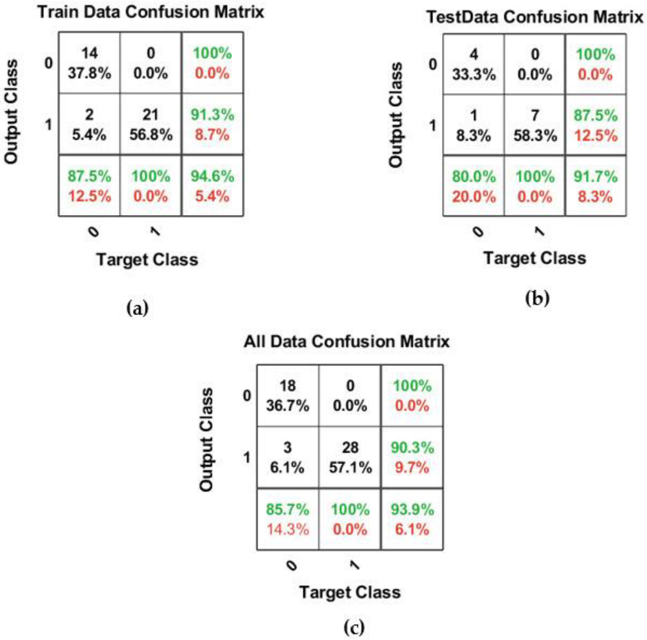
By modeling different trial and error techniques, the best structure of the binary classification model with k*_0.3 = 0.3 was determined when the SP, MNL, and MNNL are equal to 0.6, 15, and 5, respectively. According to the results of binary classification for the first scenario with k*_0.3 = 0.3, this developed model was able to identify and determine a very suitable mapping between input and output data. The model structure assumes the MNL and MNNL equal to 5 and 15, correspondingly. The developed model could correctly predict and classify 18 nodes H < H_s with the label “0”. Additionally, 28 and 3 nodes could be predicted and classified correctly and wrongly, respectively. Finally, this model could predict and classify the total dataset with an accuracy equal to 93.9%.

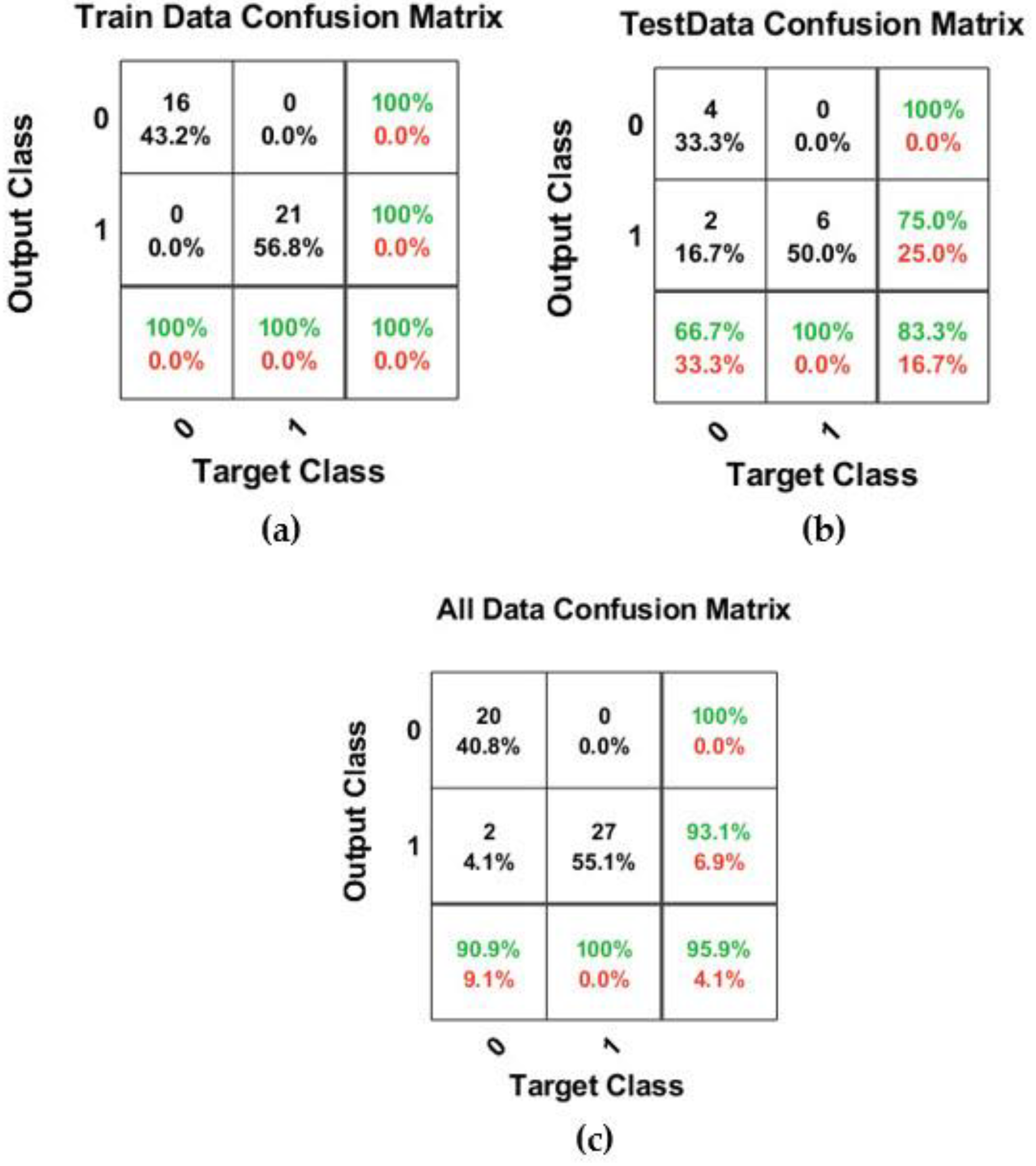
The best structure of the binary classification model with k*_1.0 = 1.0 was determined as the SP, MNL, and MNNL equal to 0.6, 15, and 10, respectively. Compared to the structure of the best model with k*_1.0 = 1.0, there is no significant change and only the value of MNNL has changed. The best-developed binary classification model could predict with 100% accuracy for training data and 83.3% accuracy for testing data. Consequently, the total accuracy of this model was 95.9% that 47 nodes were correctly predicted and only 2 nodes were wrongly predicted.

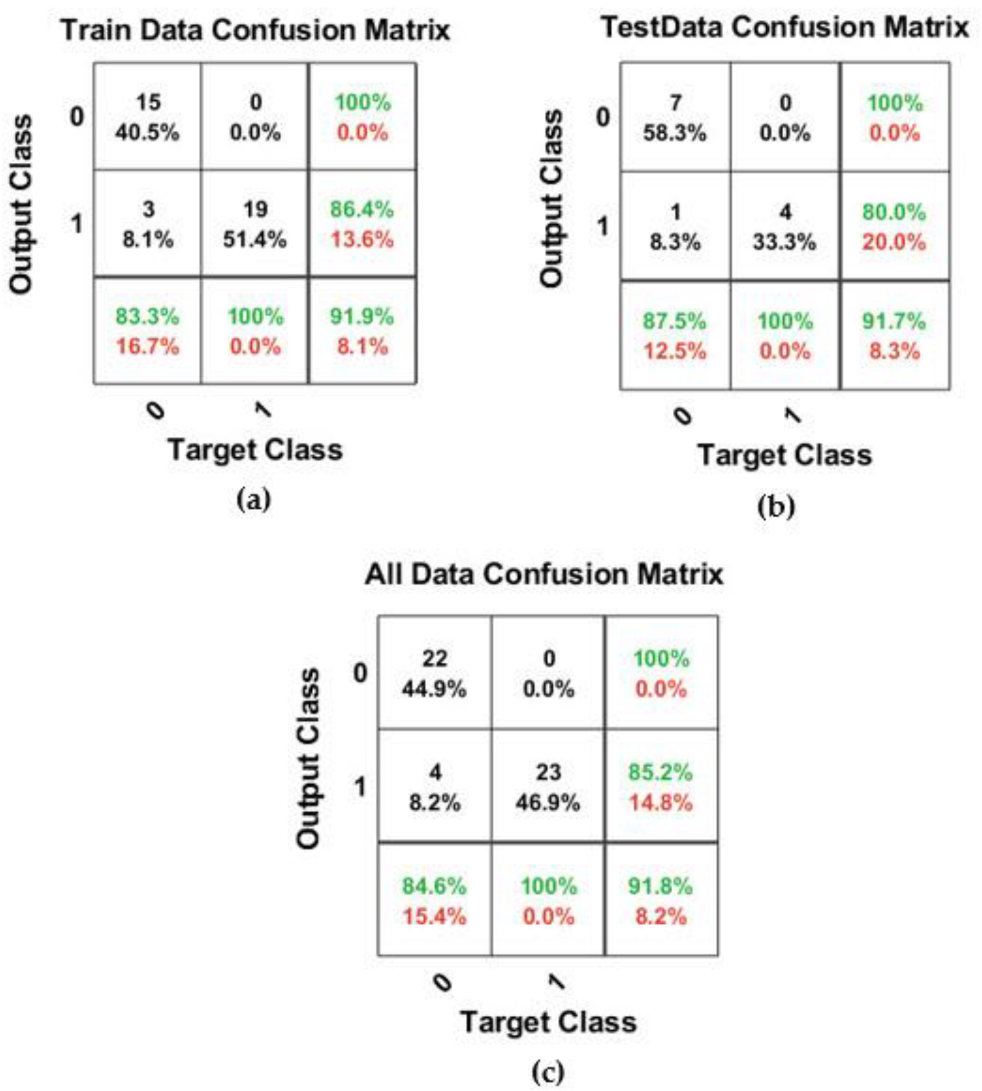
In the last scenario with k*_1.8 = 1.8 after many modelings, the results showed that the structure of the best model was similar to the structure of the best model for k*_1.8 = 1.8. The accuracies of training and testing data were 91.9% and 91.7%, respectively. This model could predict 22 nodes (H < H_s) with the label “0” as correct with 100% accuracy in all data. Additionally, from 27 nodes (H ≥ H_s) with the label “1”, 23 nodes were correctly predicted, and the rest was predicted incorrectly. Therefore, this model was able to predict the total amount of data with 91.8% accuracy. Finally, it was found that the binary classification approach can provide suitable performance capacity in predicting the performance of water distribution networks for k*_0.3 = 0.3, k*_1.0 = 1.0, and k*_1.8 = 1.8.

5. Results and Discussion

In the first step, the behavior of the water distribution network of Spezzano Albanese in Southern Italy was analyzed with the PDA approach acquiring data to perform the GMDH model. The developed models were constructed for three scenarios (k*_i).

Table 3. Comparison of the three structures of best classification models for three scenarios.

No. Scenario	k*i	Selection Pressure (SP)	Maximum Number of Layers (MNL)	Maximum Number of Neurons in a Layer (MNNL)
1	0.3	0.6	15	5
2	1	0.6	15	10
3	1.8	0.6	15	10

and

Table 4. Values of F*_i,Train, F*_i,Test and F*_i,Total assuming k*_0.3 = 0.3, k*_1.0 = 1.0 and k*_1.8 = 1.8.

No. Scenario	k*i	F*i-Train	F*i-Test	F*i-Total
1	k*0.3 = 0.3	94.6	91.7	93.9
2	k*1.0 = 1.0	100	83.3	95.9
3	k*1.8 = 1.8	91.9	91.7	91.8

show the three structures of best classification models for the three scenarios and a comparison of their results, respectively. It is necessary to mention that in this section to conduct a sensitivity analysis, the F* is used to present the results of accuracy of Train, Test, and Total for modeling with k*_0.3 = 0.3, k*_1.0 = 1.0, and k*_1.8 = 1.8. Furthermore, the F is considered for Train, Test, and Total to show the results of accuracy for modeling with the different values of k*_j,i.

After determining the structures of best classification models for the three scenarios with k*_0.3 = 0.3, k*_1.0 = 1.0, and k*_1.8 = 1.8, the best model for each k*_i is modeled varying this value: the change in the percentage of k_i* is between 80% and 120% with units of 5%

Assuming the different values of k*_j,i, F*_j,i-Train, F*_j,i-Test, F*_j,i-Total were calculated. Furthermore, the values of sensitivity functions (F*_j,i − F_i*)/F_i* for each of them (Train, Test, Total) were also calculated.

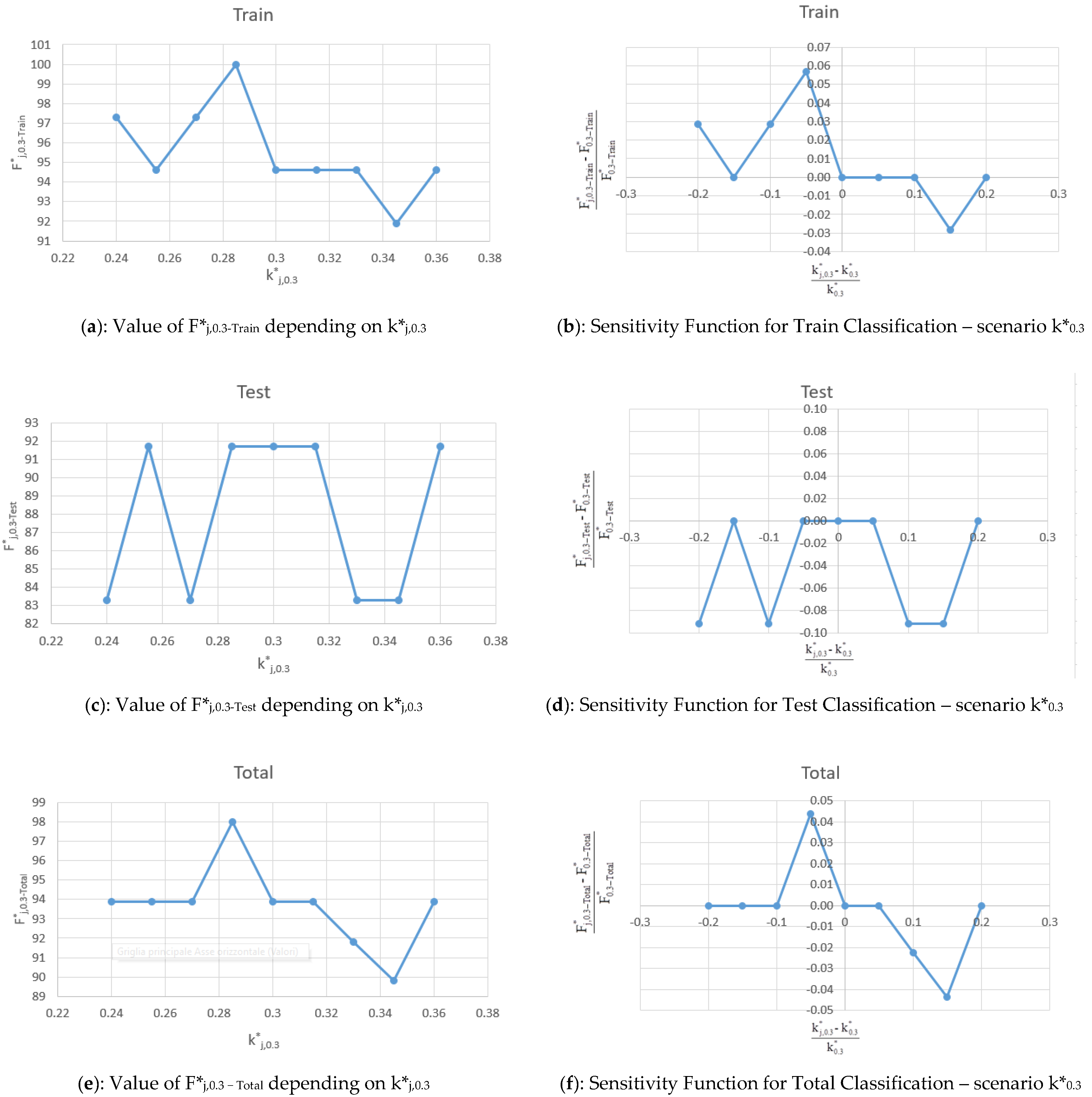
5.1. Scenario k*_0.3

The values of F*_j,0.3-Train, F*_j,0.3-Test, F*_j,0.3-Total, and sensitivity function (F*_j,0.3 − F*_0.3)/F*_0.3 for Train, Test and Total obtained varying k*_0.30 = 0.30 in the range are shown in

Table 5. Values of F*_j,0.30-Train, F*_j,0.30-Test, and F*_j,0.30-Total by varying k*_0.30 in the fixed range.

k*j,0.3	%	F*j,0.3-Train	$\frac{{\mathbf{F}}_{\mathbf{j},0.3\text{-}\mathbf{Train}}^{*}-{\mathbf{F}}_{0.3\text{-}\mathbf{Train}}^{*}}{{\mathbf{F}}_{0.3\text{-}\mathbf{Train}}^{*}}$	F*j,0.3-Test	$\frac{{\mathbf{F}}_{\mathbf{j},0.3\text{-}\mathbf{Test}}^{*}-{\mathbf{F}}_{0.3\text{-}\mathbf{Test}}^{*}}{{\mathbf{F}}_{0.3\text{-}\mathbf{Test}}^{*}}$	F *j,0.3-Total	$\frac{{\mathbf{F}}_{\mathbf{j},0.3\text{-}\mathbf{Total}}^{*}-{\mathbf{F}}_{0.3\text{-}\mathbf{Total}}^{*}}{{\mathbf{F}}_{0.3\text{-}\mathbf{Total}}^{*}}$
0.24	80	97.3	0.03	83.3	−0.09	93.9	0.00
0.255	85	94.6	0.00	91.7	0.00	93.9	0.00
0.27	90	97.3	0.03	83.3	−0.09	93.9	0.00
0.285	95	100	0.06	91.7	0.00	98.0	0.04
0.3	100	94.6	0.00	91.7	0.00	93.9	0.00
0.315	105	94.6	0.00	91.7	0.00	93.9	0.00
0.33	110	94.6	0.00	83.3	−0.09	91.8	−0.02
0.345	115	91.9	−0.03	83.3	−0.09	89.8	−0.04
0.36	120	94.6	0.00	91.7	0.00	93.9	0.00

and in terms of sensitivity plot in the Figure 9a–f.

The values of each F*_j,0.3 (Train, Test, Total) are good: all values are higher than 91.9% for Train, 83.3% for Test, and 89.8% for Total. This confirms the quality of the results and the model accuracy. The sensitivity function assumes values that confirm the stability of the model results because the sensitivity function is always lower than 10%. If the input value of k*_i is slightly different, due to an error or variability in a real case, the models furnish very similar results.

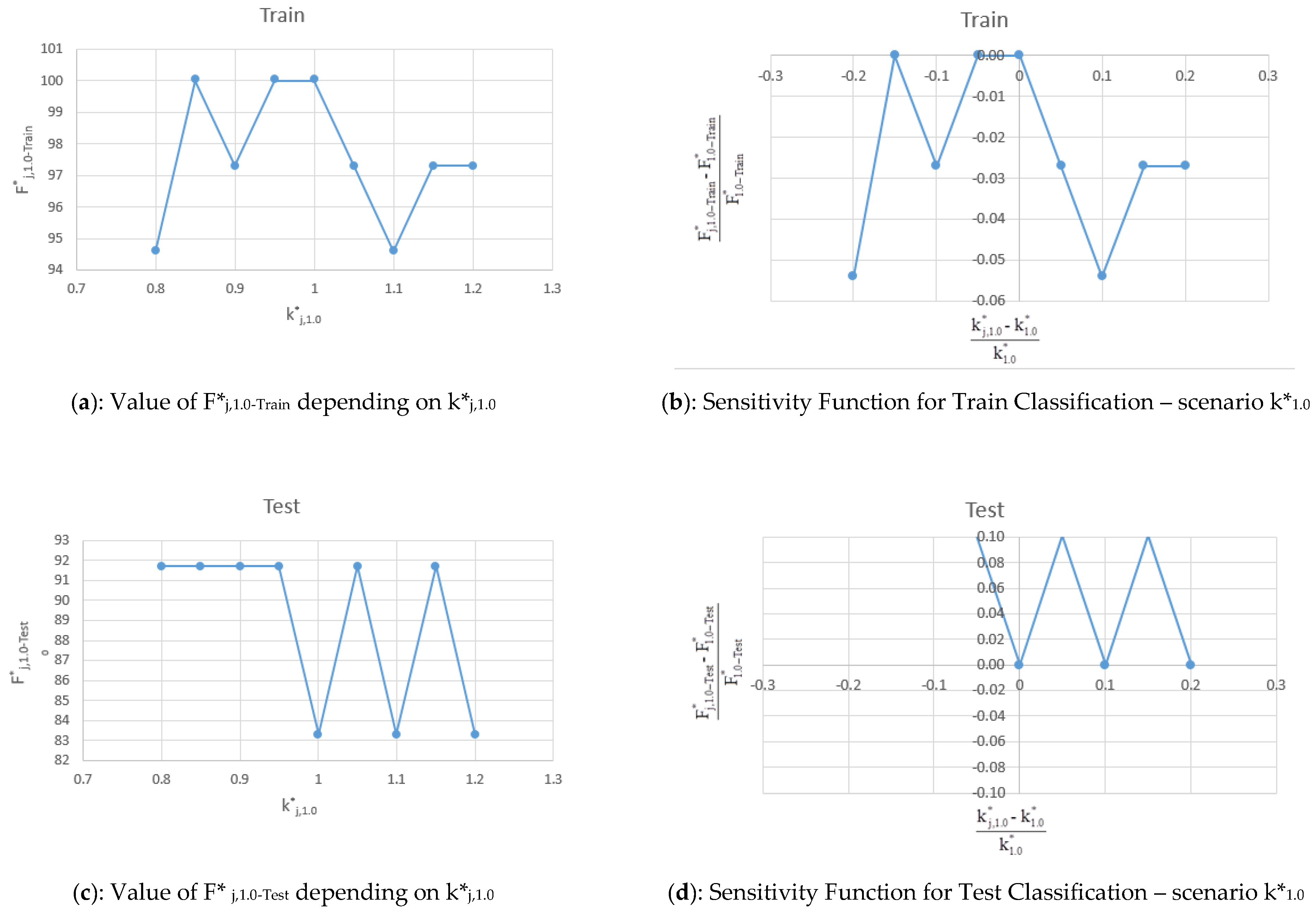
5.2. Scenario k*_1.0

The values of F*_j,1.0-Train, F*_j,1.0-Test, F*_j,1.0-Total and sensitivity function (F*_j,1.0 − F*_1.0)/F*_1.0 for Train, Test and Total obtained varying k*_1.0 = 1.0 in the range are shown in

Table 6. Value of F*_j,1.0-Train, F*_j,1.0−Test, and F*_j,1.0-Total by varying k*_1.0 in the fixed range.

k*j,1.0	%	F*j,1.0-Train	$\frac{{\mathbf{F}}_{\mathbf{j},1.0\text{-}\mathbf{Train}}^{*}-{\mathbf{F}}_{1.0\text{-}\mathbf{Train}}^{*}}{{\mathbf{F}}_{1.0\text{-}\mathbf{Train}}^{*}}$	F*j,1.0-Test	$\frac{{\mathbf{F}}_{\mathbf{j},1.0\text{-}\mathbf{Test}}^{*}-{\mathbf{F}}_{1.0\text{-}\mathbf{Test}}^{*}}{{\mathbf{F}}_{1.0\text{-}\mathbf{Test}}^{*}}$	F*j,1.0-Total	$\frac{{\mathbf{F}}_{\mathbf{j},1.0\text{-}\mathbf{Total}}^{*}-{\mathbf{F}}_{1.0\text{-}\mathbf{Total}}^{*}}{{\mathbf{F}}_{1.0\text{-}\mathbf{Total}}^{*}}$
0.8	80	94.6	−0.05	91.7	0.10	93.9	−0.02
0.85	85	100	0.00	91.7	0.10	98	0.02
0.9	90	97.3	−0.03	91.7	0.10	95.9	0.00
0.95	95	100	0.00	91.7	0.10	98	0.02
1	100	100	0.00	83.3	0.00	95.9	0.00
1.05	105	97.3	−0.03	91.7	0.10	95.9	0.00
1.1	110	94.6	−0.05	83.3	0.00	91.8	−0.04
1.15	115	97.3	−0.03	91.7	0.10	95.9	0.00
1.2	120	97.3	−0.03	83.3	0.00	93.9	−0.02

and in terms of sensitivity plot in Figure 10a–f.

By assuming k*_1.0 the values of each F*_j,1.0 (Train, Test, Total) are also good. The F*_j,1.0 values are higher than 94.6% for Train, 83.3% for Test, and 91.8% for Total. This is in agreement with the k*_0.3 case and confirms the goodness of both the results and the model accuracy.

The sensitivity function assumes values that confirm the stability of the model results because the sensitivity function is always lower than 10% and, in the case of Train and Total, are below 5%.

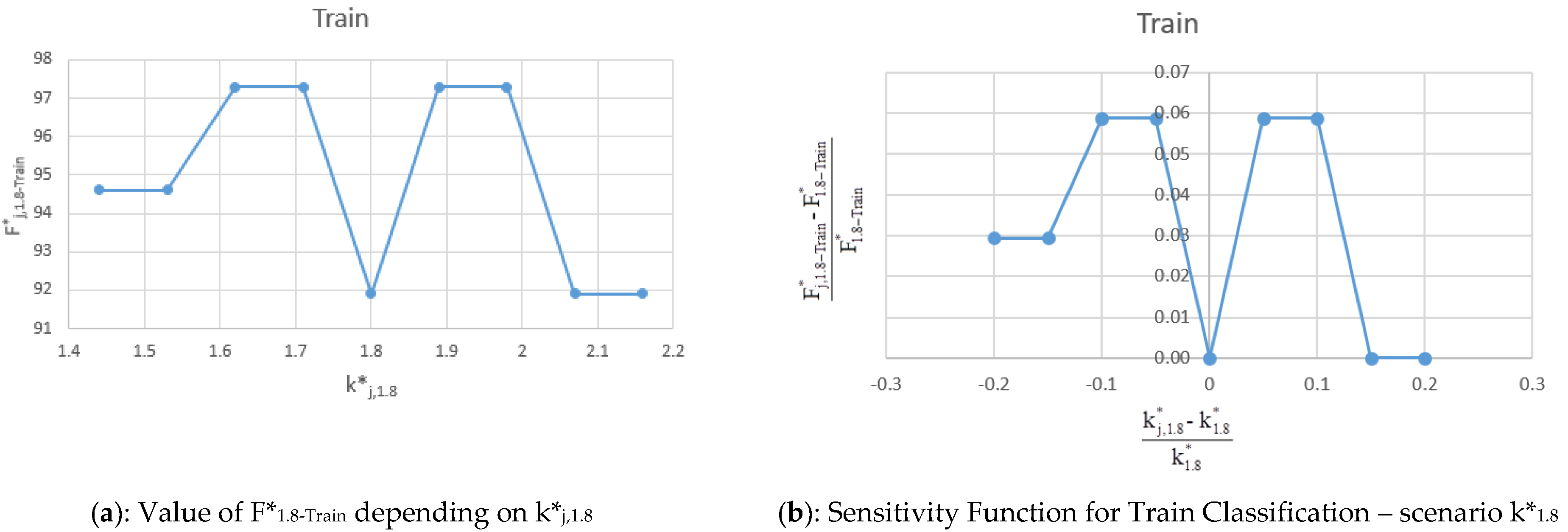
5.3. Scenario k*_1.8

The values of F*_j,1.8-Train, F*_j,1.8-Test, F*_j,1.8-Total and sensitivity function (F*_j,1.8 − F*_1.8)/F*_1.8 for Train, Test and Total obtained varying k*_1.8 = 1.8 in the range are shown in

Table 7. Values of F*_j,−0-Train, F*_j,1.80-Test, and F*_j,1.80-Total by varying k*_1.80 in the fixed range.

k*j,1.8	%	F*j,1.8-Train	$\frac{{\mathbf{F}}_{\mathbf{j},1.8\text{-}\mathbf{Train}}^{*}-{\mathbf{F}}_{1.8\text{-}\mathbf{Train}}^{*}}{{\mathbf{F}}_{1.8\text{-}\mathbf{Train}}^{*}}$	F*j,1.8-Test	$\frac{{\mathbf{F}}_{\mathbf{j},1.8\text{-}\mathbf{Test}}^{*}-{\mathbf{F}}_{1.8\text{-}\mathbf{Test}}^{*}}{{\mathbf{F}}_{1.8\text{-}\mathbf{Test}}^{*}}$	F*j,1.8-Total	$\frac{{\mathbf{F}}_{\mathbf{j},1.8\text{-}\mathbf{Total}}^{*}-{\mathbf{F}}_{1.8\text{-}\mathbf{Total}}^{*}}{{\mathbf{F}}_{1.8\text{-}\mathbf{Total}}^{*}}$
1.44	80	94.6	0.03	91.7	0.00	93.9	0.02
1.53	85	94.6	0.03	83.3	−0.09	91.8	0.00
1.62	90	97.3	0.06	91.7	0.00	95.5	0.04
1.71	95	97.3	0.06	83.3	−0.09	93.9	0.02
1.8	100	91.9	0.00	91.7	0.00	91.8	0.00
1.89	105	97.3	0.06	83.3	−0.09	93.9	0.02
1.98	110	97.3	0.06	83.3	−0.09	93.9	0.02
2.07	115	91.9	0.00	83.3	−0.09	89.8	−0.02
2.16	120	91.9	0.00	83.3	−0.09	89.8	−0.02

and in terms of sensitivity plot in Figure 11a–f.

The results of the analysis are confirmed for the k*_1.8 scenario. F*_j,1.8 values for Train, Test, and Total are all higher than 89.8%. These results do not differ from previous ones and confirm the quality of the results and the model accuracy.

6. Conclusions

In this study, a novel sensitivity analysis was presented to evaluate the behavior of WDNs analyzed by the PDA approach and the classification technique by using an appropriate artificial neural network, namely the GMDH. Through the analysis, the design peak coefficient k*, a significant parameter for customer adequacy in water supply networks, was successfully evaluated in terms of binary classification. For practical application, the proposed methodology was applied to the water distribution network of Spezzano Albanese in Southern Italy using a PDA approach to analyze the network and the classification technique by the GMDH algorithm to test the results.

The results applying the proposed methodology show that the GMDH results and the Epanet output for each scenario do not change significantly. It means that the model is stable, and the k* values adopted in the design of the network are correct for management purposes.

The accuracy of the best developed binary models for k*_0.3 = 0.3, k*_1.0 = 1.0, and k*_1.8 = 1.8 were 93.9%, 95.9%, and 91.8% for all data, respectively. It was found that the binary classification approach demonstrates its high capability in the prediction and evaluation of WDNs. The comparison between the best classification models for the different values of each k*_i showed the high capability of the model in predicting the performance of water distribution networks and the sensitivity analysis confirms that the results are stable.

For future works, other researchers and engineers can use a combination of EPANET software and the GMDH algorithm to evaluate the behavior of other real WDN with different characteristics with sensitivity analysis. Finally, the network behavior could be evaluated with other binary classification algorithms before subsequently comparing results.