
Evaluation of Incipient Motion of Sand Particles by Different Indirect Methods in Erosion Function Apparatus


1
Agricultural Facilities Engineering Laboratory, Graduate School of Agriculture, Kyoto University, Kitashirakawa-Oiwakecho, Sakyo-ku, Kyoto 606-8502, Japan
2
Rural Development Academy (RDA), Bogura 5842, Bangladesh
*
Author to whom correspondence should be addressed.
Water 2021, 13(8), 1118; https://doi.org/10.3390/w13081118
Submission received: 16 March 2021
/
Revised: 12 April 2021
/
Accepted: 14 April 2021
/
Published: 19 April 2021
(This article belongs to the Special Issue Sediment Transport and River Morphology)
Abstract
:An experiment was carried out in an acrylic glass-sided re-circulating closed conduit with a rectangular cross section, which is similar in construction to an erosion function apparatus. An adjustable sand box, made of acrylic glass, was attached to the bottom of the conduit as the sand zone or the test section. The hydraulics of the flow in the erosion function apparatus is complicated due to the limited part of the non-smooth and erodible soil surface attached to the closed conduit. As the bed shear stress changes with the bed roughness, even though the flow velocity does not change, establishing a method to estimate the incipient motion is an important challenge for an erosion function apparatus. The present study was conducted to explore the incipient motion of sands from bed shear stress estimated by four different indirect methods on both the sand bed and the smooth bed installed in the erosion function apparatus. In the experiment, particle image velocimetry (PIV) was used to investigate flow dynamics and incipient motion in terms of dimensionless critical bed shear stress. The experimental results show that the bed shear stress estimated from the log-law profiles in the sand zone and the smooth zones are relatively higher than those of the other indirect methods. The dimensionless critical bed shear stress of threshold condition evaluated by all indirect methods was found in good agreement with those of previous results in both zones. The Manning roughness and Darcy–Weisbach friction coefficients were evaluated based on the critical shear velocity at the incipient motion. Although these coefficients were found slightly greater in the smooth zone than in the sand zone, in both zones, they showed good agreement with previous studies.
1. Introduction
1.1. Threshold Shear Stress in Erosion Function Apparatus (EFA)
When erodible solid particles of a sediment bed are exposed to a shearing flow of a Newtonian fluid such as air or water, the bed particles may be set in motion by the action of flow forces and then transported by the flow, initiating a process called erosion [1]. One of the classical problems in the field of erosion is to predict or evaluate the flow strength (bed shear stresses) at which sediment motion first begins. This condition for incipient motion is usually known as critical shear stress or threshold shear stress. Incipient motion of sediment is one of the main aspects of the sedimentation process, and it can, in theory, be realized and predicted from a balance of the forces acting on the sediment particles [2,3]. Shields [4] conducted pioneering study, and the equation proposed by him is widely accepted and used in engineering practice in studies on fluvial hydraulics. The incipient motion problem can be considered either as the minimum shear stress required to initiate a given particle or as the largest grain size that can be lifted by a given shear stress. Researchers in the field of hydraulics and geoenvironmental engineering prefer the first concept, whereas geologists prefer the latter concept. Briaud et al. [5] developed the erosion function apparatus (EFA) in the form of a closed conduit to quantify the erosion rate of fine grained soils, although the EFA can also be adopted to quantify the erosion rate of coarse grained soils if necessary. The bed shear stress applied at the soil–water interface by flowing water is calculated using the Moody diagram and the measured flow velocity [5,6]. The following equation is adopted to estimate bed shear stress in EFA by flowing water.
where is the bed shear stress, f is the friction factor obtained from the Moody diagram, is the mass density of water and v is the mean flow velocity.
The erosion rate is predicted in the form of an erosion function curve by plotting the recorded erosion rate and computed bed shear stress. The critical shear stress or threshold shear stress is determined by extending the prediction line of the erosion function curve at zero erosion rate. While the Moody diagram is a suitable engineering tool in hydraulics, it has some important practical limitations [7]. First, it is only rigorously accurate for surfaces in which the equivalent sand roughness height is known previously and that are operating in the fully rough regime [7]. The equivalent sand roughness height is a function of shear velocity for a particular liquid and the surfaces in EFA may not always lie in the fully rough regime. In addition, only the limited part of the bottom of the pipe in EFA is rough or non-smooth, while the other parts of the pipe are smooth. As a result, the bed shear stress changes with the bed roughness, even though the flow velocity does not change. The magnitude of the bed shear stress in EFA varies in the range of 0.1–10 Pa; hence, the bed shear stress is indirectly determined from the mean flow velocity. However, it is not easy to obtain accurate estimations of the bed shear stress because the hydraulics of the flow in the EFA is complicated due to the limited part of the non-smooth and erodible soil surface. Therefore, establishing a method to estimate the bed shear stress in EFA is an important challenge that remains to be overcome.
1.2. Threshold Shear Stress in Other Experimental Facilities
The critical shear stress at incipient motion of cohesionless sediment particles has been explored experimentally by many researchers [8] under a unidirectional flow in closed conduit and open channel. Southard and Boguchwal [9] reported the dimensionless boundary shear stress against dimensionless sediment size and observed a decrease in bed shear stress in the transition from dunes to plane bed with increasing flow velocity. Costello and Southard [10] conducted flume experiments with four sizes of coarse sand to study geometry, migration and hydraulics of bed configurations. They found that the ripple field narrows with increasing sand size at low flow velocities whereas, dunes are found to exist in a stable phase for all sand sizes. Rees [11] also conducted flume experiments and established a relationship between the magnitude of the tangential stress and the upstream slope of a bed of fine silt. Sundborg [12] investigated fluvial sediments and fluvial morphology both experimentally and theoretically and observed the state of sediment movement, particularly with the influence of grain size and density on the transport processes. Ashley [13] reported the relationship between the sediment size and bedforms size and found that bedform superposition with sediment size can be used to describe more thoroughly the variety of subaqueous dunes in nature. Contrarily, the use of the Shields diagram [4] has its limitations, in terms of predicting incipient motion, due to a few conditions, such as uniform distribution of sediments, horizontal or near-horizontal sediment bed slopes and unidirectional flows. The authors of [14,15,16] discussed the ratio of the critical shear stress on a slope to that on a horizontal bed to the angle of the slope. The authors of [17,18,19] developed a threshold condition for sediments of a non-uniform size. Wilcock [20] stated that the shear velocity is a fundamental variable in river studies for calculating the sediment transport, scour and deposition. Even though several indirect techniques are available for determining shear velocity, none are universally accepted [21]. Many researchers (e.g., [22,23,24,25,26,27]) verified turbulence measurements by using acoustic doppler velocimeter (ADV) and laser doppler anemometer (LDA) in rivers and laboratory flumes. Tominaga and Sakaki [26] tested several methods of evaluating shear velocity from mean velocity and turbulence statistics by using ADV. Along similar lines, particle image velocimetry (PIV) is also a promising technique at present, which provides instantaneous measurements of the flow velocity. It is also worth mentioning that most of the available experimental and numerical studies (e.g., [27,28,29,30,31]) discuss turbulence statistics in detail at immobile bed condition. Although the mobile bed condition is more obvious and practical in an open-channel flow, it is not easy to conduct experiment in mobile bed condition. Hence, there is still room to improve accuracy of bed shear stress estimation on the mobile bed, and it is necessary to undertake further investigations considering the motion of bed particles.
1.3. Importance of Resistance Coefficients in EFA and Other Experimental Facilities
Recently, numerical simulations have become a powerful tool for predicting changes in the river bedforms and flow structures due to flow dynamics. It is crucial to know the resistance characteristics in order to obtain accurate numerical simulations of sediment transport in rivers.
The Manning roughness coefficient and Darcy–Weisbach friction coefficient or the equivalent grain roughness are usually considered according to an adopted resistance law in two- or three-dimensional flow simulations [26]. It is usually difficult to estimate such coefficients in real scale due to the limitations of the experiments. Although it is possible to connect field studies and laboratory investigations through scaling laws and, sometimes, numerical simulations, it is common to determine the resistance coefficient in EFA and similar experimental facilities in the laboratory conditions of the bed material. Thus, it is essential to estimate such resistance coefficients based on the shear velocity or bed shear stress in laboratory experiments.
The above descriptions summarize the importance of determining the shear velocity and, subsequently, the bed shear stress to compute incipient motion and later on resistance coefficients in EFA and other experimental facilities. We investigated the incipient motion of sand particles by different turbulent statistics (indirect methods), such as log-law, Reynolds shear stress and turbulent intensity from the measured velocity profiles using PIV. Since the laboratory flume in this study includes a limited mobile sand bed on its smooth acrylic bed as well as EFA, the evaluation of the shear velocity can elucidate significant changes on both types of beds. To the best of the authors’ knowledge, no study has been reported yet for estimating the incipient motion of sand particles on the different types of beds estimated by different indirect methods for PIV employed experimentation. Therefore, this experimental investigation provides informative results for indirect determination of the bed shear stress. The objective of the present study was to determine the incipient motion and resistance coefficient, during the slow motion of bed particles by a number of indirect methods in two beds, namely the sand zone (rough bed) and the upstream edge of the sand zone (smooth acrylic bed), in EFA. The rest of this paper is arranged as follows. The experimentation along with the procedures and mathematical derivations for various methods of calculation for the shear velocity are presented in Section 2. Then, the results are discussed in Section 3. The paper ends with the conclusions.
2. Materials and Methods
2.1. Experiment and Procedure
The experimental setup and test material were the same as those used in [32], although it did not include the water tank to generate the seepage flow. The experiment was carried out in an acrylic glass-sided recirculating closed conduit or channel of 300 cm in length, 10 cm in width and 5 cm in height, with no bed slope. An adjustable sand box (10 cm × 10 cm in cross section and 21.5 cm in height), made of acrylic glass, was fixed to the bottom of the conduit as the sand zone or the test section. The test section was located 201.5 cm downstream of the conduit. Water was pumped to recirculate in the conduit by a centrifugal pump. A valve was used to control the flow rate of the conduit, and it was monitored using an electromagnetic flow meter. A transparent sand trap, 10 cm in width and 13 cm in depth, was placed 14.5 cm downstream of the sediment zone to collect the transported sand particles as the deposition box during the experiment. The test apparatus was essentially the same as the EFA used in [5], although it did not include the deposition box. The test apparatus for the experiment is shown in Figure 1. Black cohesionless silica sand, non-uniform in size, whose particles had a median diameter of 0.58 mm and a grain density of 2.64 g/cm3, was used as the test material. Cohesionless sand was packed in the sand box as the sediment bed of the conduit.
At the beginning of the test, the sediment box was filled with cohesionless sand particles and installed at the bottom of the conduit. The water flow into the main conduit was started and maintained at a slow rate so as not to set in motion the sediment particles. The motion of the sediment particles started as the flow rate in the main channel was gradually increased. Then, side view images were acquired, focusing on the target zones (the smooth zone and the sand zone) using PIV, as shown in Figure 1, for subsequent analysis of the vertical velocity vector profiles and turbulence statistics of the closed conduit flow for each flow rate. The sediment transport was recorded for 30–60 min and collected from the deposition box. Then, the wet sand particles were dried in an oven at 120 °C for 24 h. By measuring the weight of the dried sand particles, the sediment transport rate was obtained for each run. Eight flow rates were performed for this experiment. Table 1 shows the experimental conditions.
2.2. Indirect Methods to Estimate Shear Velocity
Since the direct measurement of the bed shear stress is quite difficult, it is found that the bed shear stress can be evaluated from velocity measurements by using various methods in the literature (e.g., [22,24,26,33,34]). The velocity distribution of the flow is divided into two regions, namely, inner and outer, with two distant sets of characteristics such as velocity and length scales in turbulent boundary layers. In the inner region, closest to the bed, the bed shear stress, , is the appropriate scale, and the characteristic length scale is . Here, are the shear velocity and kinematic viscosity of water, respectively. We employed different methods: using vertical distributions of the primary mean velocity, the Reynolds shear stress and the turbulence intensity distributions. Although these methods are applicable for two-dimensional prismatic open-channel flows, we tested their applicability for the present closed conduit similar to EFA. We determined directly shear velocity contrary to bed shear stress for simplicity from available different formulas and then calculated bed shear stress. The different estimation methods of bed shear stress are described as follows.
2.2.1. Log-Law Method
The universal logarithmic law is expressed as follows for boundary layer problems:
where is the mean velocity, is the von Karman constant, y is the vertical coordinate from the bed surface and is the integration constant. The origin of the y coordinate was set to the roughness top by visually recognized images using the particle image velocimetry (PIV) method. As for the constants, k = 0.41 and B = 5.29 were adopted as suggested in [35] for smooth beds. However, it is common to find different k and B values in the literature, e.g., k variations of 0.38 < k < 0.45 and B variations of 3.5 < B < 6.1 [21,36]. Considering the equivalent grain roughness, , Equation (2) can be written as
According to the Tominaga and Sakaki [26], Equation (3) can be rearranged to
A linear regression equation can be found from the measured velocity profile on the semi-logarithmic plot as follows
where is the slope and is the intercept of the equation. Comparing Equations (4) and (5), the shear velocity and the equivalent grain roughness are calculated as
The shear velocities obtained by curve fitting to Equation (2) and the linear regression analysis of Equation (3) are denoted as and , respectively.
It is important to note that Equation (2) is only applicable to the acrylic bed (smooth zone) at the upstream edge of the sand zone, whereas Equation (3) is applicable to the sand zone. Although the log-law-based methods are most popular for estimating the shear velocity, the applicability of the log-law is limited to parts of the flow that are close to the wall (<20% of the height of the flow [37]). Furthermore, the log-law-based methods are critically dependent on precise knowledge of the profile origin above the sand bed, which is very sensitive to the velocity gradient.
2.2.2. Reynolds Shear Stress Method
In the outer region of the fully developed turbulent flow with a high Reynolds number, the viscous term contribution becomes negligible, and the Reynolds shear stress asymptotically approaches the following equation [34]:
where are the turbulent fluctuating velocities in the x and y directions, respectively, and d is the water depth. It should be noted that the water depth and apparatus depth were the same in this study. Equation (8) implies that the Reynolds shear stress is distributed linearly across the channel, and it can be used to predict the shear velocity. The shear velocity was obtained by extrapolating the measured profiles to the bed. The shear velocity estimated by this method is denoted as . It should be noted that the distribution of the Reynolds shear stress is liable to be affected by secondary currents and form drag due to roughness elements [26,38]. Tominaga and Sakaki [26] also mentioned that the measurement of the Reynolds shear stress distribution is relatively difficult in field conditions because it is liable to be affected by various local flow structures.
2.2.3. Turbulence Intensity Method
It is well known that the turbulence intensities follow the universal profiles proposed in [39] in the two-dimensional open-channel flows reported in [26]. The equations to determine the shear velocity are given as follows
where are the turbulent intensities in the x, y and z directions, respectively, and are known as the root mean squares of the fluctuation velocities in the x, y and z directions, respectively. The shear velocities estimated by data fitting to Equations (9) and (10) are designated as and . It was not possible to calculate the turbulent intensity in the z direction due to the limitation of the current PIV instrumentation, although only the streamwise component (in the x direction) is important for analyzing flow dynamics. Turbulence intensity is an important quantity for many physical phenomena such as laminar–turbulent flow transition, development of the turbulent boundary layer and the position of flow separation [39,40,41,42]. It also provides important information in field measurements more easily than the Reynolds shear stress distribution [26].
3. Results and Discussion
3.1. Streamwise Flow Velocity in Closed Conduit
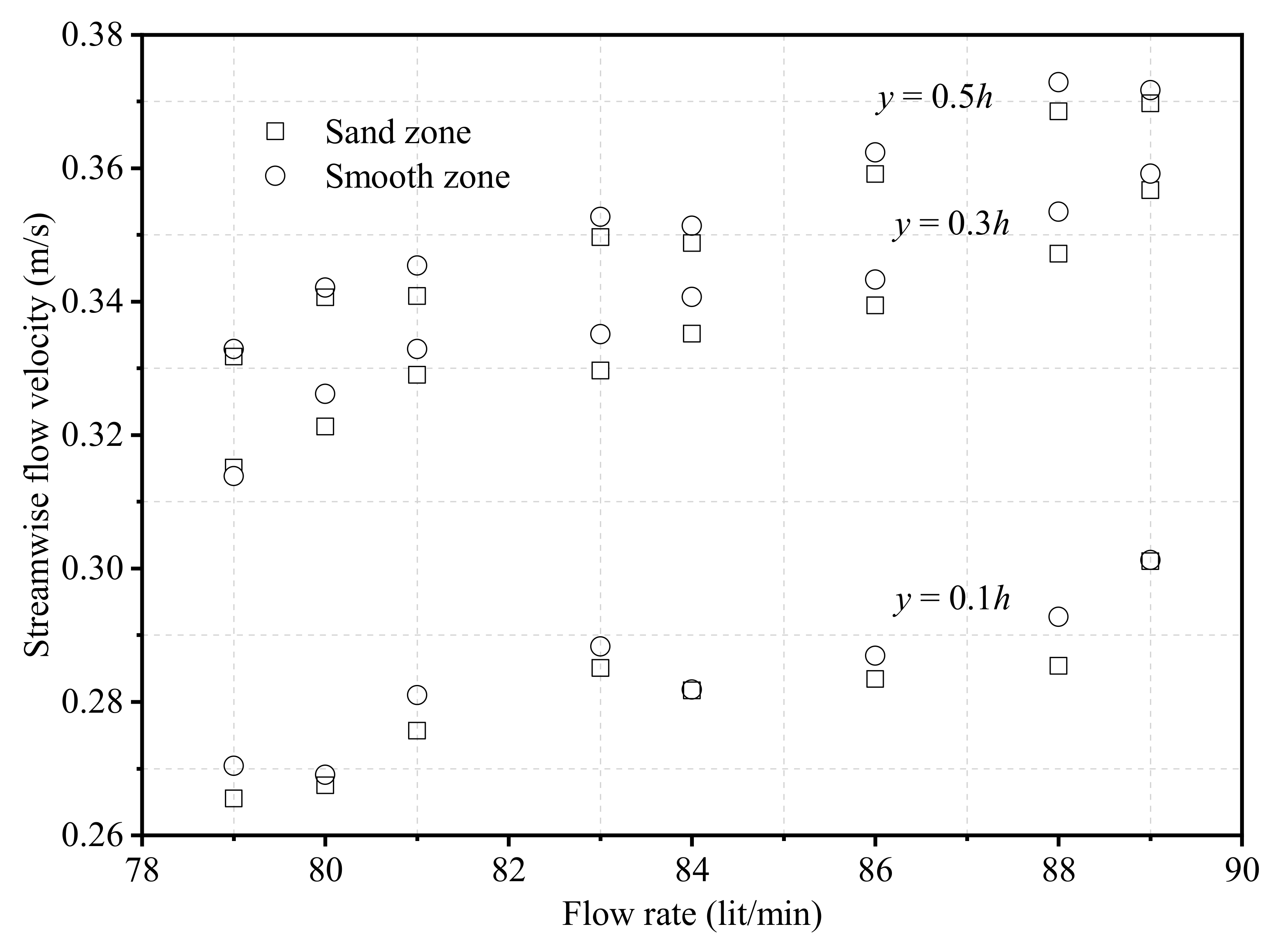
Figure 2 shows the streamwise vertical velocity profiles at y = 0.1h, y = 0.3h and y = 0.5h (where, ) in the sand zone and the smooth zone, respectively.
Since it is a closed conduit and because of symmetricity, the streamwise flow velocity is considered only from bottom to center of the conduit. It shows that the streamwise velocity decreases in the sand zone at different depths although the flow rate in the closed conduit is the same. Although the flow velocity difference is small between the sand zone and smooth zone, such small difference can cause significant change of turbulent quantities. It is apparent that the profiles shift more sharply at y = 0.3h and y = 0.5h than at y = 0.1h. The computed velocity variations are tabulated in Table 2 for both zones.
3.2. Universal Characteristics of Turbulence Flow in Closed Conduit
The universal distributions of the turbulence quantities, such as the mean velocity, Reynolds shear stress, turbulent intensity, etc. of the flow, were investigated for both the sand zone and the smooth zone. Then, the bed shear stress using shear velocity was calculated using the methods described in Section 2.2.
3.2.1. Logarithmic Distributions of Flow Profiles
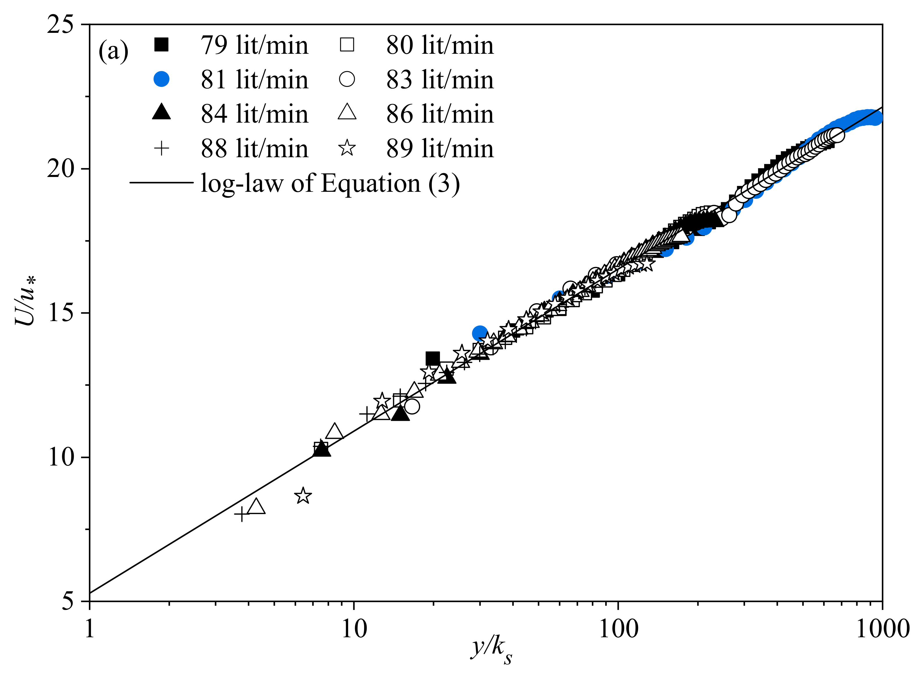
The vertical distributions of the primary mean velocity are shown in Figure 3 for both zones. The solid lines are the log-law profiles of Equations (2) and (3). One indirect technique for calculating the shear velocity in the sand zone is a regression analysis of the measured velocity profile. The analysis employs Equation (3) and then Equation (6) to determine the shear velocity. The equivalent grain roughness can also be calculated from Equation (7). Then, the primary mean velocity and the vertical distance of the flow are non-dimensionalized by the calculated shear velocity and the equivalent grain roughness, as presented in Figure 3a. The figure shows that the log-law distribution is well fit for all the vertical distance values irrespective of the different flow rates.
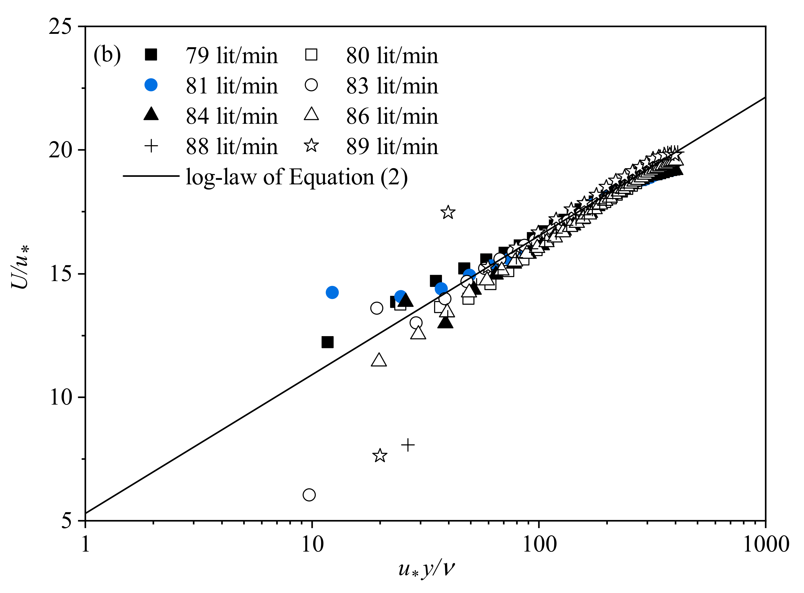
Another indirect technique for calculating the shear velocity is the curve-fitting of the measured velocity profile to the logarithmic law of Equation (2) at the upstream edge of the sand zone or smooth zone calculated by the Newton–Raphson iterative method. Then, the primary mean velocity of the flow is non-dimensionalized by the determined shear velocity, whereas the vertical distance is non-dimensionalized by the viscous length scale, as shown in Figure 3b. Figure 3b shows that the log-law distribution is applicable for almost all the considered vertical distances in all of the flow rates. The velocity near the bed departs from the log-law more than that at the rest of the depth, as shown in Figure 3b.
Since the experiment was focused on the slow motion of the bed particles, the mean flow velocity was gradually changed for each flow rate, which caused small variations in the calculated data for both zones. Nevertheless, both indirect techniques agree well with the log-law for both zones.
3.2.2. Reynolds Shear Stress Distribution of Flow Profiles
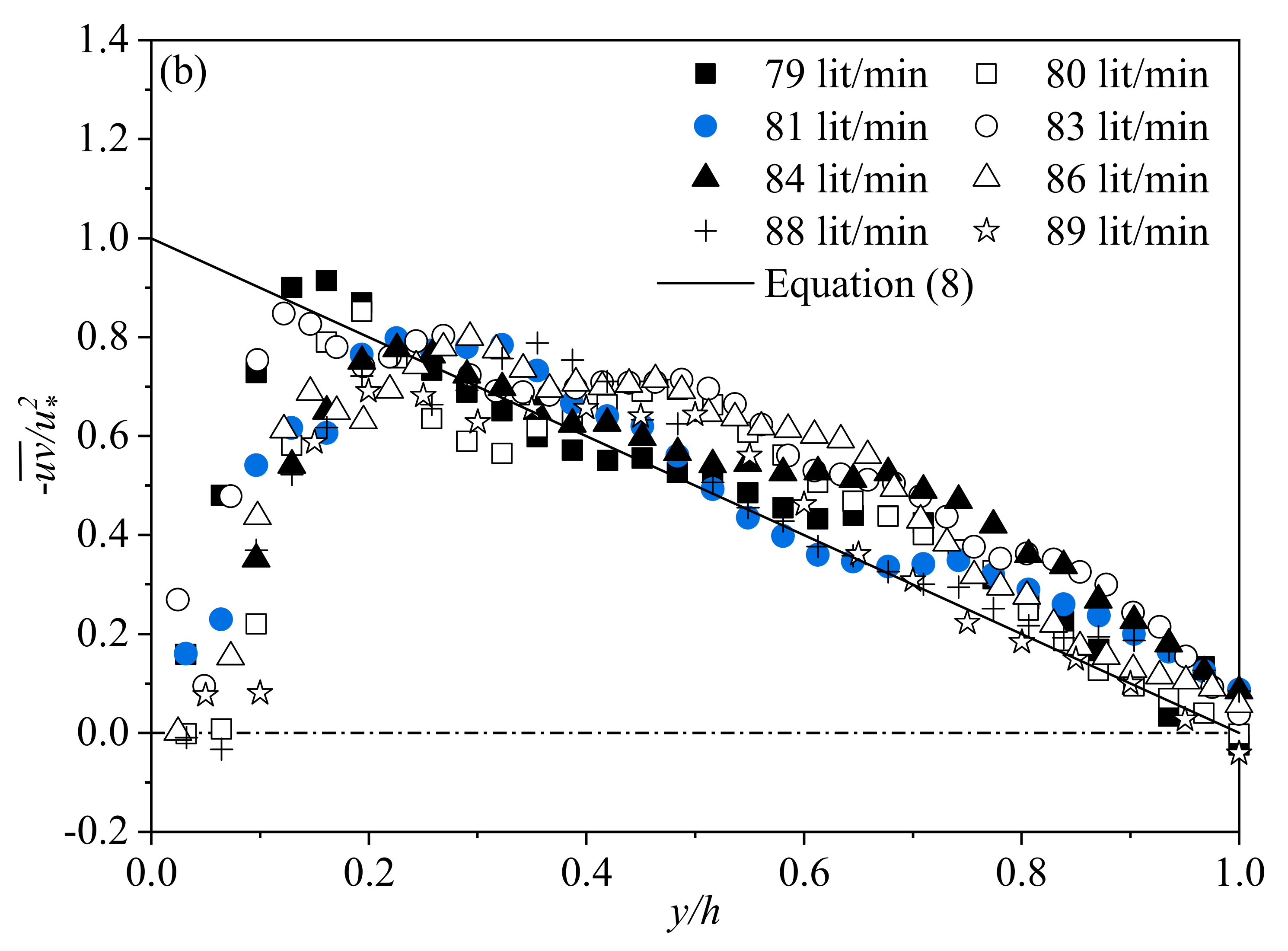
The vertical distributions of the Reynolds shear stress non-dimensionalized by the evaluated shear velocity are shown in Figure 4a,4b for the sand zone and the smooth zone, respectively. The figure shows that the Reynolds shear stress distributions oscillate around the liner distribution calculated by Equation (8). The distributions reach a maximum near the bed around y/h = 0.1 and then decrease linearly to the center of the channel. Since it is a closed conduit flow, the same Reynolds shear stress distributions are found for the top wall.
It was found that the distributions for all the flow rates form a triangular shape, as shown in Figure 4a, although the triangular shape is more visible for the distributions at the smooth zone, as shown in Figure 4b.
As all the profiles in the sand zone have uniform distributions and they agree well with the linear distributions, the shear velocity can be calculated by linear extrapolation, as shown in Figure 4a. Figure 4b shows that the distributions for all the flow rates are minimum very close to the bed, reach the maximum at around y/h = 0.2 and then linearly decrease to the center of the channel. It is also noticeable that the distributions are well fitted to the linear distribution line of Equation (8). Since the distributions form a triangular shape and are uniform rather than scattered, the shear velocity can also be estimated by linear extrapolation, as shown in Figure 4b.
3.2.3. Turbulence Intensity Distribution of Flow Profiles
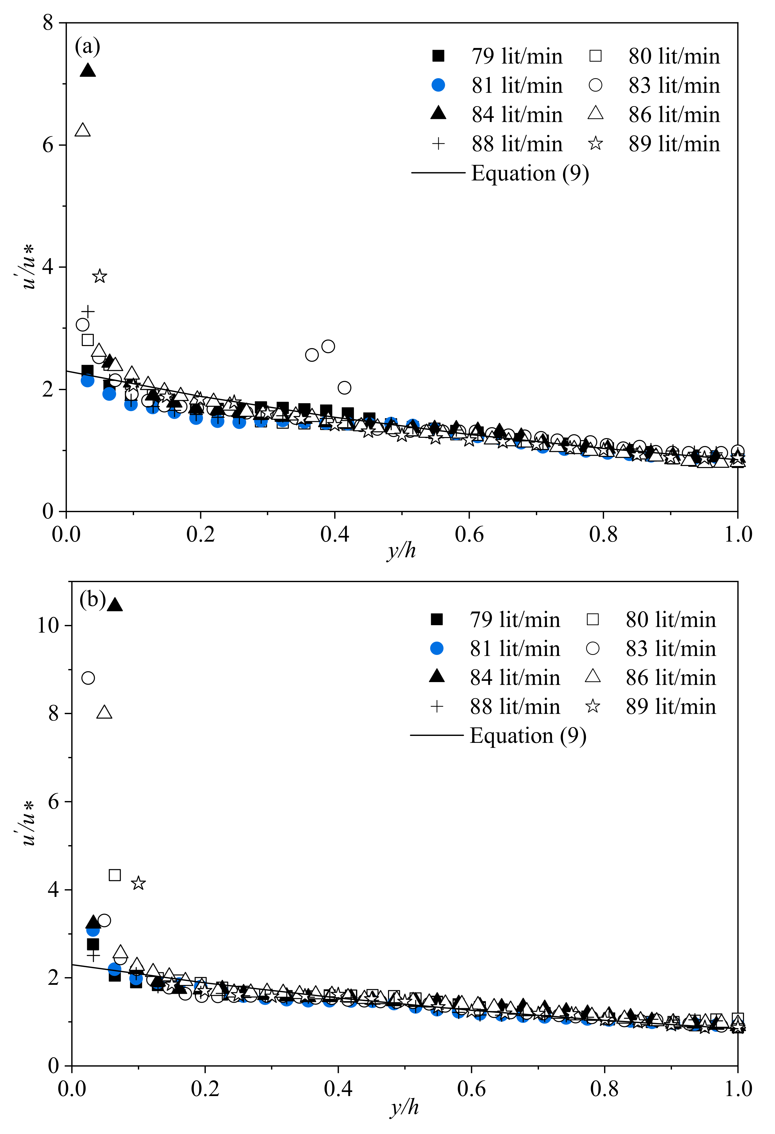
The non-dimensionalized distributions of turbulence intensities considering the x-component of the flow are shown in Figure 5 for both the sand zone and the smooth zone. The distributions are fairly unfluctuating and the degree of conformity between the estimated data and Equation (9) is plainly high through the depth of flow in both zones. The streamwise turbulence intensity in both zones is found to be at the maximum close to the bed regardless of the flow rates, as shown in Figure 5a,b.
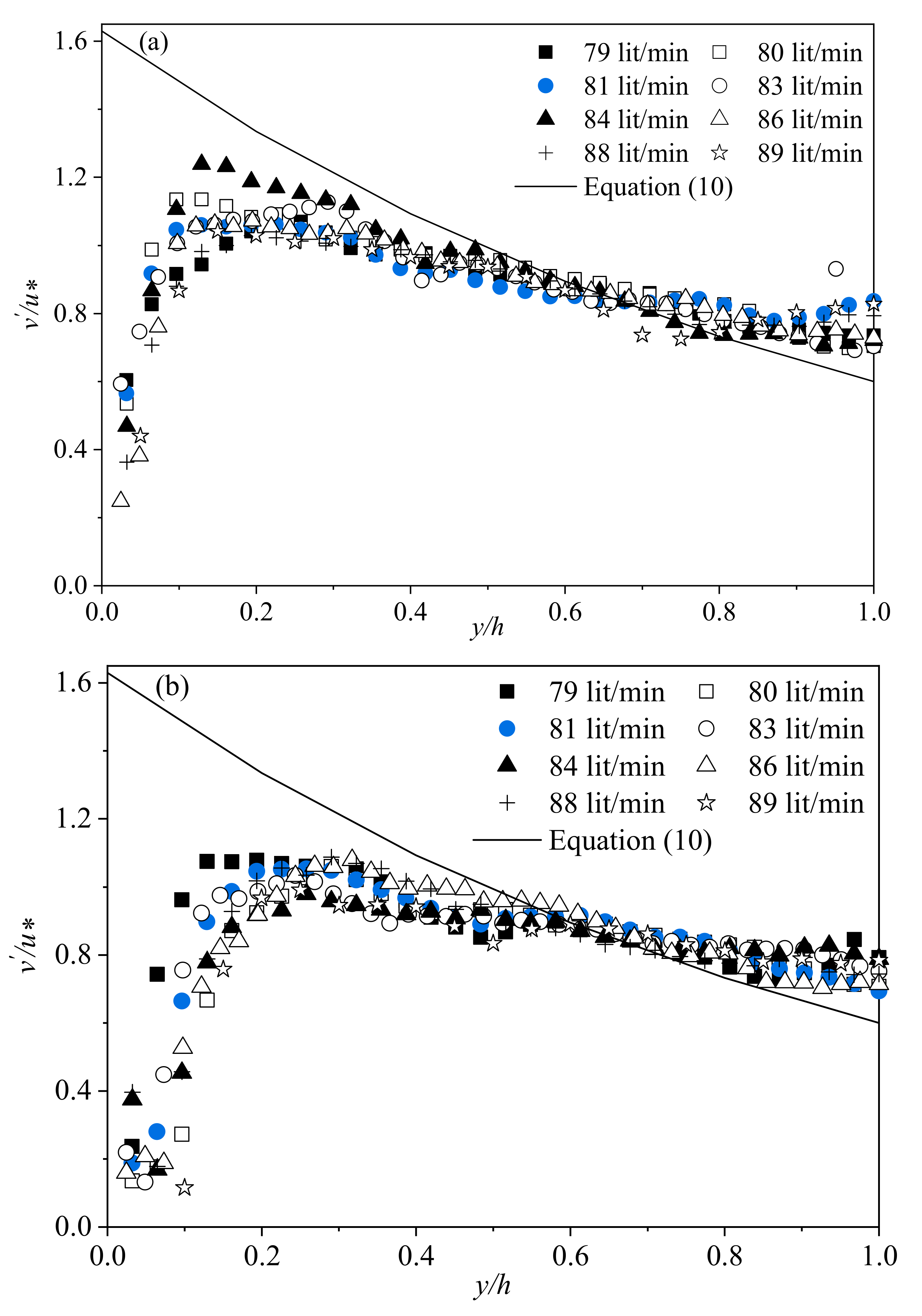
The non-dimensionalized distributions of turbulence intensities considering the y-component of the flow are shown in Figure 6 for both the sand zone and the smooth zone. In both zones, the vertical turbulence intensity is found to be at the minimum very close to the bed, and it continues to increase until the plateau-shaped local maximum around y/h = 0.2 regardless of the flow rates, as shown in Figure 6a,b. Then, the profiles decrease linearly towards the center of the channel and stay constant around = 0.8. The authors of [38,43] also observed a rather broad plateau of vertical turbulence intensities in the overlapping region for smooth wall profiles.
3.3. Shear Velocity and Bed Shear Stress of Flow
Table 3 shows the shear velocities and corresponding bed shear stresses estimated by the different indirect methods: regression analysis of the universal logarithmic law (RLL), ; Reynolds shear stress (RSS), ; turbulence intensity considering the x-component of the flow (Tix), ; turbulence intensity considering the y-component of the flow (Tiy), ; and curve-fitting to the universal logarithmic law (CLL), . The corresponding bed shear stresses calculated by above mentioned methods are denoted as and .
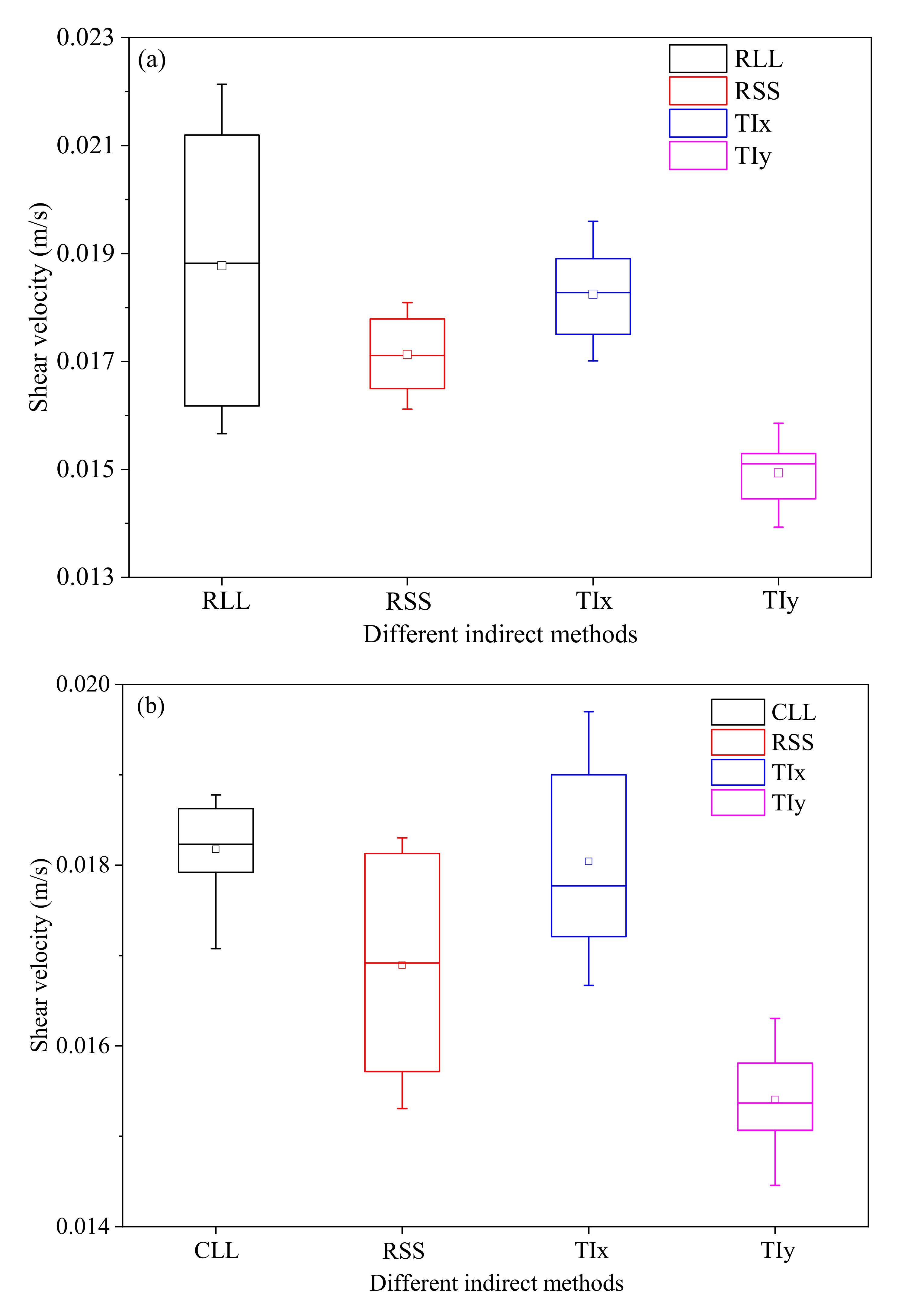
The estimated average shear velocity in sand zone for all methods except the Tiy method is more than that of smooth zone, as shown in Table 3. However, the difference between average shear velocity is small among different estimation methods in both zones. Figure 7a,b shows the variations in shear velocity for each flow rate evaluated by different indirect methods in the sand zone and the smooth zone, respectively. If the interquartile ranges and whiskers of the box plots in the sand zone are considered, the shear velocity estimated by the regression analysis of the universal logarithmic law is more dispersed than the other methods, as shown in Figure 7a. Contrarily, the shear velocity estimated by Reynolds shear stress is more dispersed than the other methods at the smooth zone, as shown in Figure 7b. The middle line of the box estimated by the turbulence intensity, considering the y-component of the flow lies outside of the boxes estimated by the other methods in both zones, as shown in Figure 7. This means there is likely to be a difference between the value of and the other shear velocities estimated in both zones, as shown in Table 3. The estimated shear velocity is skewed almost symmetrically for all the methods except the Tiy method, which is negatively skewed in the sand zone, as shown in Figure 7a. Contrarily, the shear velocity estimated by the turbulence intensity considering the x-component of the flow and the y-component of the flow are skewed positively at the smooth zone, as shown in Figure 7b. It should be noted that, unlike the formulas used in [12,44,45]], we used velocity profile and turbulence quantities to determine shear velocity. We did not consider formulas based on grain diameter for determining shear velocity in this study because we evaluated incipient motion from the flow dynamics of the conduit.
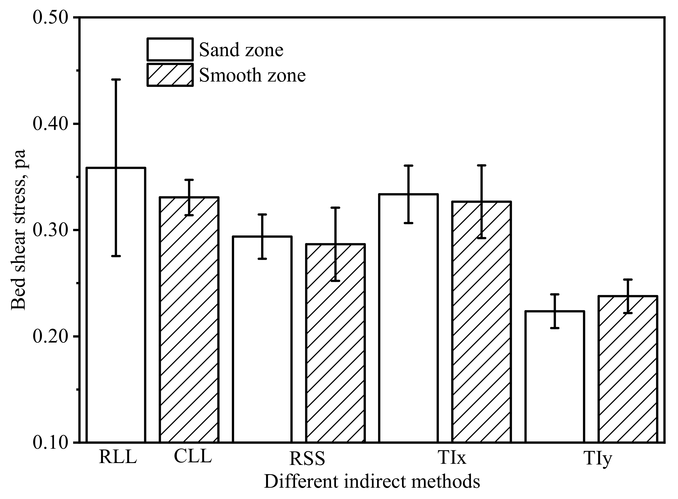
The corresponding bed shear stresses acting on the sand zone and smooth zone of the close conduit are shown in Figure 8.
The bed shear stresses estimated from the logarithmic flow profiles, i.e., , in both zones are relatively higher than that of the other indirect methods, as shown in Figure 8 and Table 3. Kim et al. [22] compared the logarithmic profile to other bed shear stress estimation methods and also found the same results. Biron et al. [46] also found very large values of bed shear stress estimated using the logarithmic law over sand bed. However, the log-law-based linear regression and curve-fitting methods are critically dependent on precise knowledge of the elevations above the sand bed, whereas the Reynolds shear stress- and turbulence intensity-based methods reduce the impact of this elevation uncertainty. Biron et al. [46] concluded that the Reynolds shear stress method is the most appropriate method. It is concluded that all the indirect methods used to evaluate the shear velocities and bed shear stresses in the sand zone and the smooth zone are reasonably acceptable. However, the estimated values by the different methods also show considerable disagreement. Here, the shear velocity and, subsequently, bed shear stress are estimated based on the measured vertical velocity profile computed from the ensemble average velocity fields by PIV. Hence, some PIV noises and errors from the instrumentation cannot be ignored. On the other hand, the regression analysis of the universal logarithmic law and curve fitting to universal logarithmic law techniques are popular for estimating the shear velocity and corresponding bed shear stress. However, these log-law-based techniques are fair, except for separating flow regions. Although the shear velocity and bed shear stress determined by all the methods comply well with each other, the real value of these quantities for both zones are still unknown.
3.4. Determination of Critical Shear Velocity
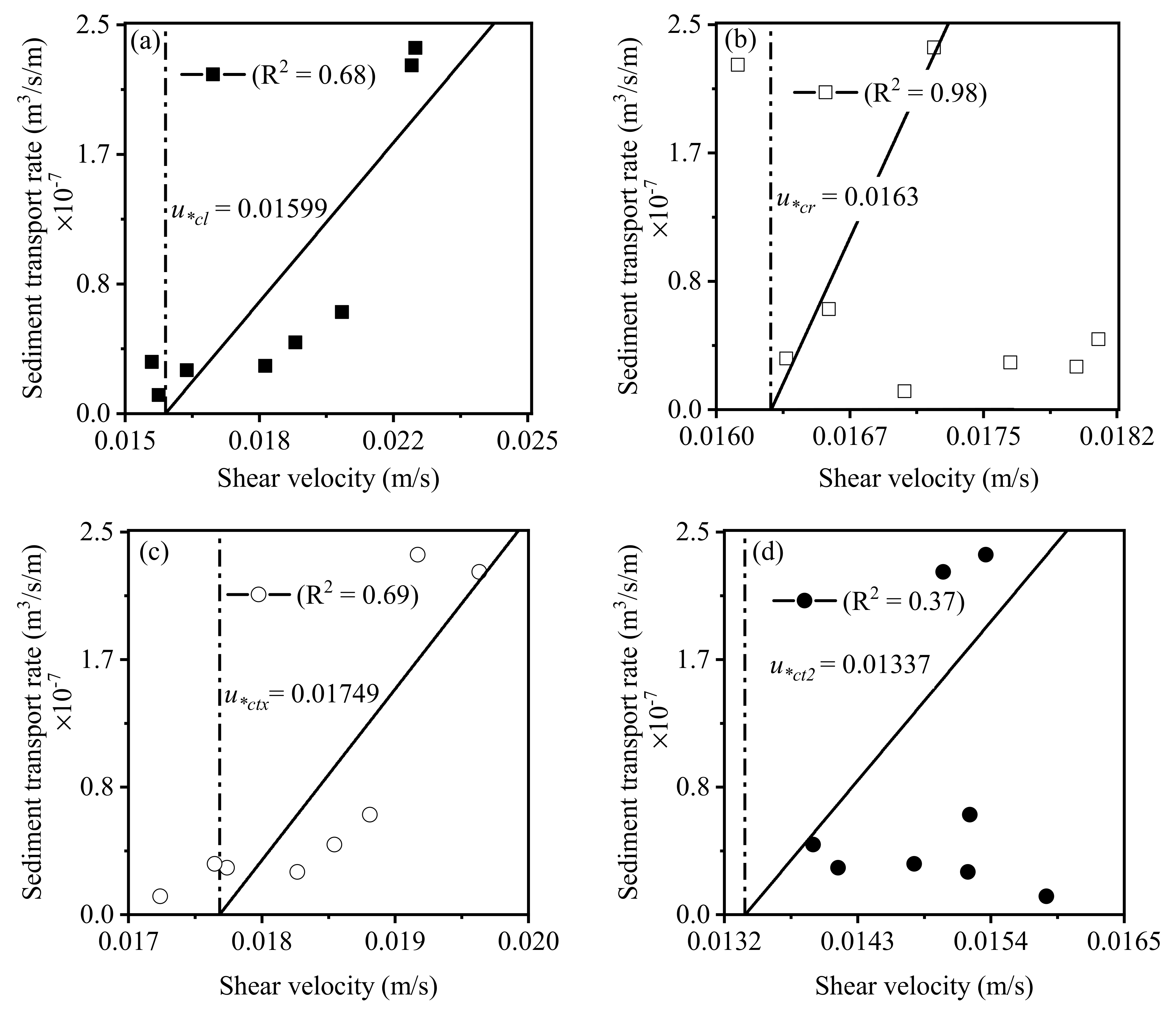
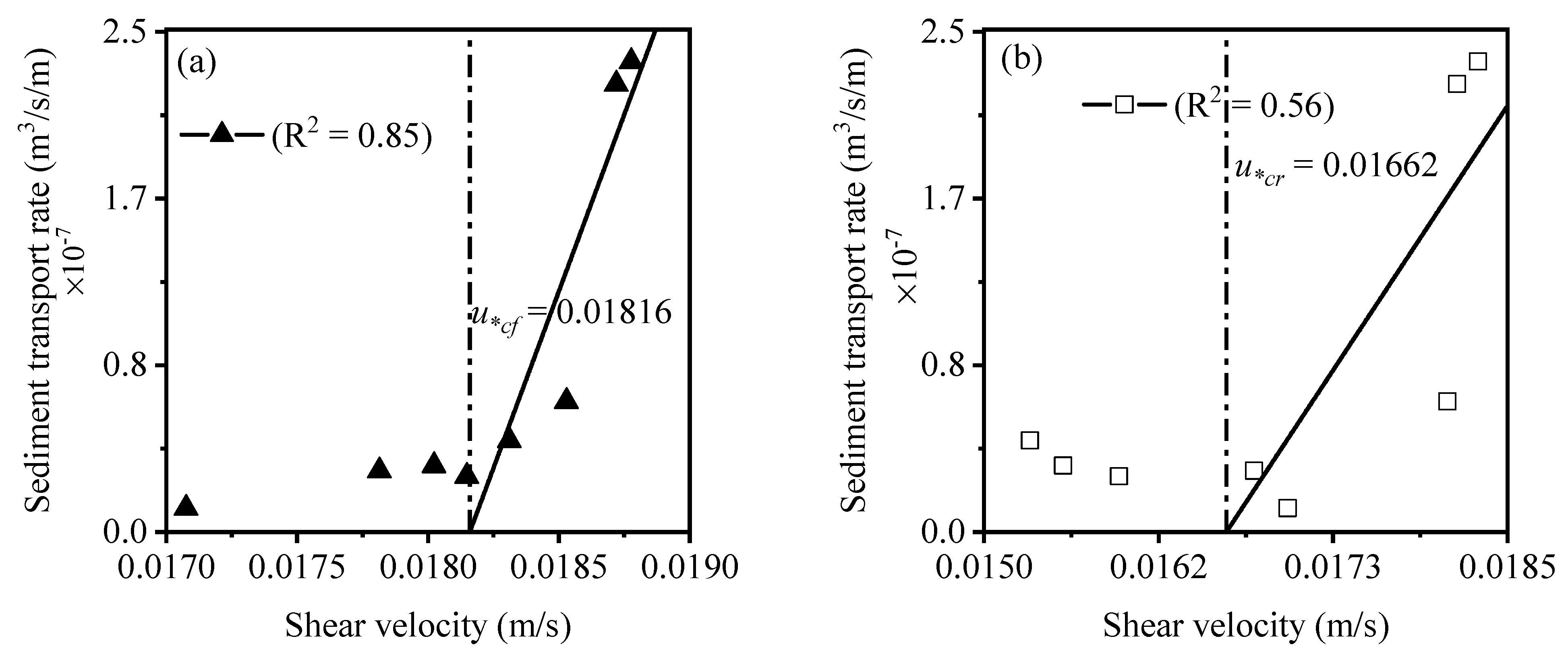
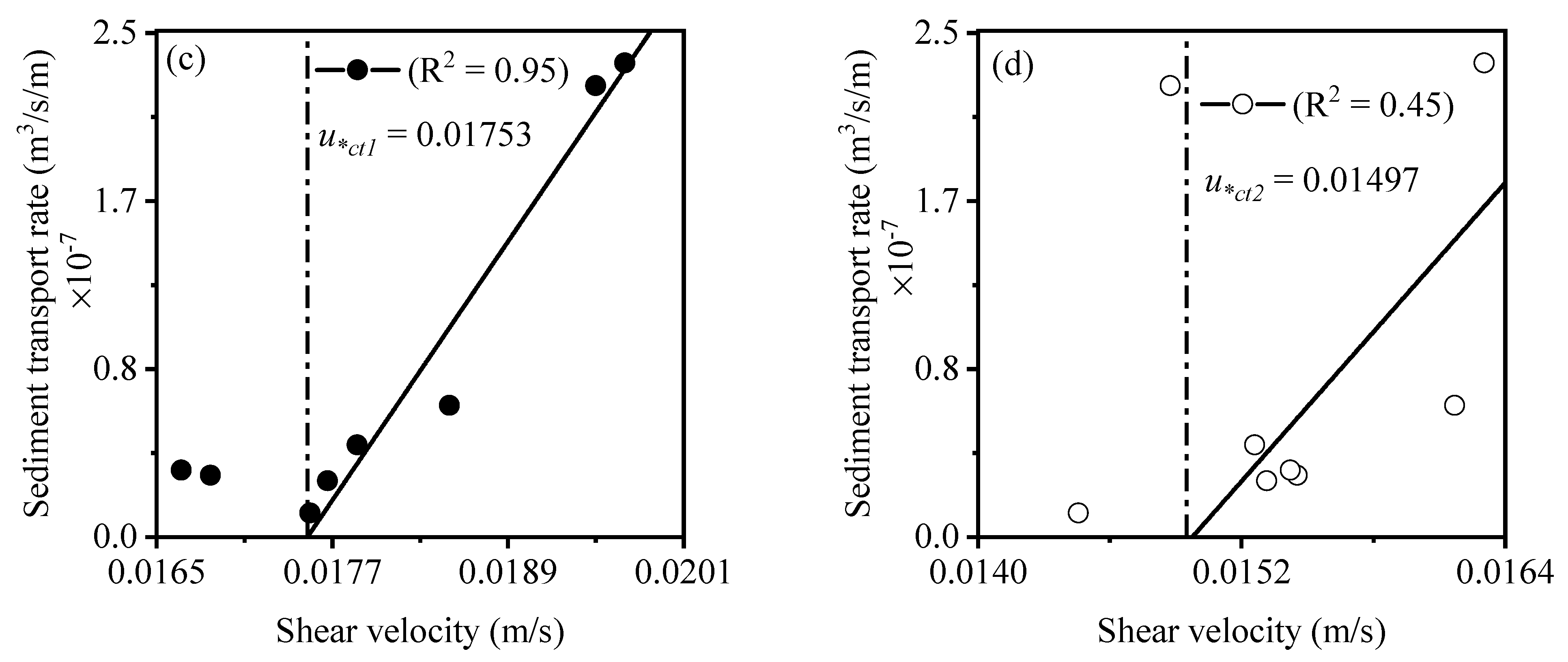
The sediment transport rates and shear velocities calculated by the different indirect methods are plotted in Figure 9 for the sand zone and Figure 10 for the smooth zone.
All figures show that the changes in the shear velocity determined by the various indirect techniques were small over the sediment transport rates. The critical shear velocity inducing the incipient motion of the sediment particles is the x-intercept obtained from the extrapolation of the prediction line fitted to higher sediment rates and corresponding shear velocities, as shown in Figure 9 and Figure 10. The value close to each vertical dashed line corresponds to the critical shear velocity for each indirect technique. The values of shear velocity estimated by different methods lie in a short range for both zones, as depicted in Table 3. Therefore, the available non-linear bedload transport equations can be linearized in the neighborhood of critical shear velocity, as shown in Figure 9 and Figure 10. We also tried the estimated bed shear stress instead of the shear velocity of different indirect methods for plotting Figure 9 and Figure 10, but the dimensionless critical bed shear stress changed negligibly. Contrarily, the shear velocity is directly related to the turbulent boundary layers of the flow. As a result, we used shear velocity to estimate critical bed shear stress and later the dimensionless critical shear stress. Correlation and ordinary regression analyses were performed to find the relationship between the shear velocity and the sediment transport rate. Each of the R-squared values is positively and significantly correlated for both zones, as shown in Figure 9 and Figure 10. They indicate a good relationship between the fitted model and the measurement. The sediment transport rate increases with the shear velocity. The critical shear velocities calculated with the different methods vary in a large range in the smooth zone in comparison with the sand zone, as shown in Table 4.
The critical shear velocities estimated by different methods such as the RLL, RSS, TIx, TIy and CLL are denoted as and respectively. Table 4 shows that the critical shear velocities in smooth zone are higher than those of the sand zone. It is worth mentioning that the differences between the values are very small. Once the critical shear velocity has been estimated, the critical bed shear stress for incipient motion of the sediment particles in EFA can be calculated, as follows:
where and denote the critical bed shear stress with the dimension of stress and the critical shear velocity, respectively.
3.5. Determination of Dimensionless Critical Bed Shear Stress
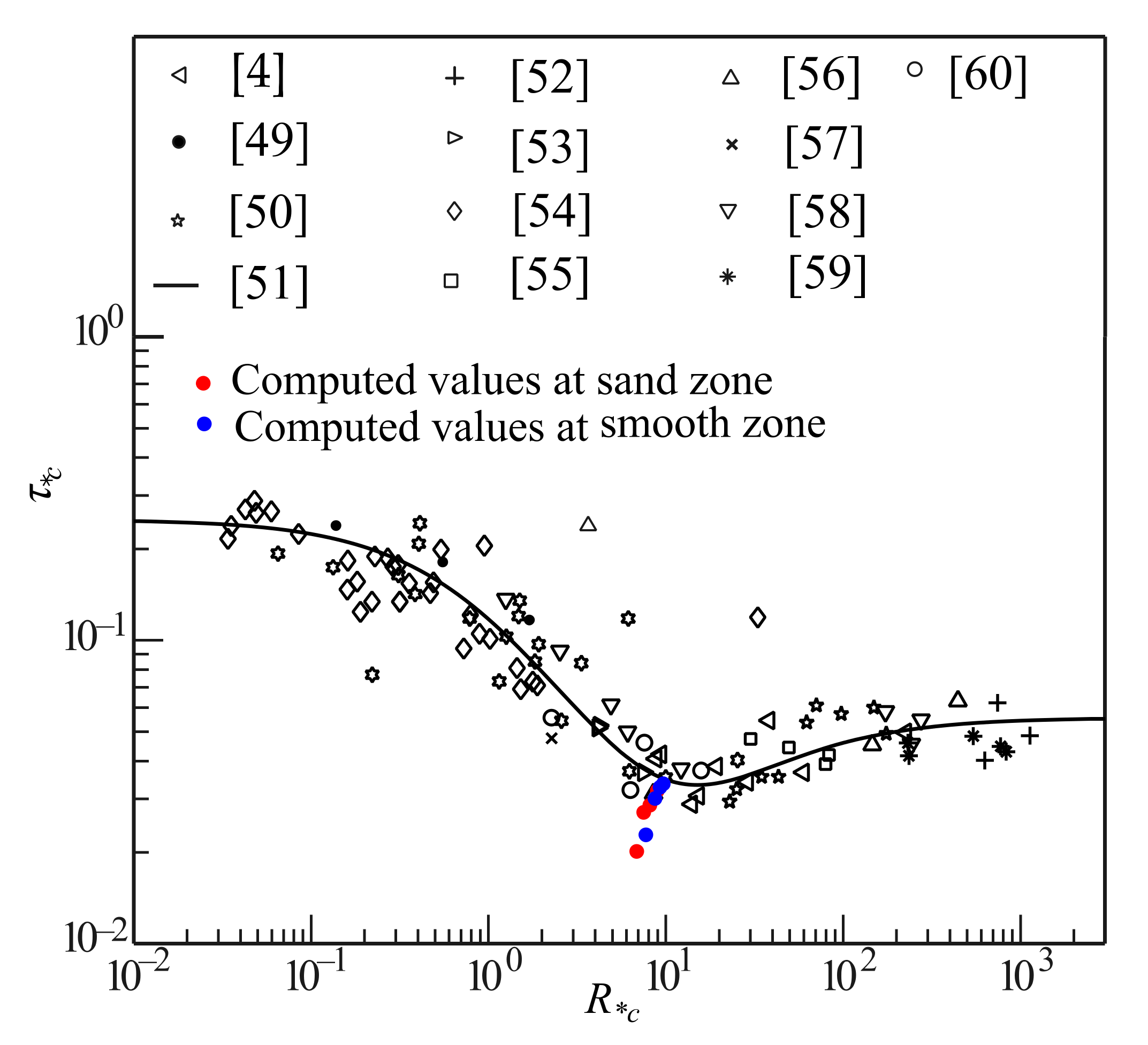
Shields [4] proposed a relationship between the dimensionless critical bed shear stress (also called the Shields parameter or the Shields entrainment function) and the critical grain Reynolds number based on the critical shear velocity to express the critical shear stress for the initiation of motion. It can be expressed as follows:
where and denote the dimensionless critical bed shear stress, the grain density, the median diameter of the cohesionless sediment particles, the critical grain Reynolds number, the kinematic viscosity of water and the gravitational acceleration, respectively. The physical meaning of the dimensionless critical bed shear stress is the ratio of the horizontal force to the vertical force exerted onto a particle on the bed where the horizontal and vertical forces are proportional to and , respectively. The dimensionless critical shear stress estimated by different methods such as the RLL, RSS, TIx, TIy and CLL are denoted as and , respectively. The estimated dimensionless critical bed shear stress of the different methods is tabulated in Table 5 for both zones.
The dimensionless critical bed shear stresses are also plotted in the Shields diagram shown in Figure 11. It was found that the estimated dimensionless critical bed shear stress varies in the range of 0.01949 ≤ ≤ 0.03533 in both zones. The values are in accordance with the Shields diagram and a good agreement was found where the value of for coarse granular material ( > 0.5 mm) is 0.033 at 20 °C [47]. The dimensionless critical bed shear stresses in the smooth zone are higher than those of the sand zone. The authors of [32] also reported higher values for the dimensionless critical bed shear stress at the upstream edge of the sand zone or smooth zone in comparison to the sand zone. The calculated values of the sublayer thickness and grain shear Reynolds number at the smooth zone are in the range of 4.08 × 10⁻⁴–1.01 × 10⁻³ m and 6.67–16.48, respectively. It means that the turbulent flow is in the range of transition which is close to the hydraulically smooth range [47]. Since the upstream edge of the sand zone is physically smooth, the downstream component of the fluid force exerted on the boundary can result only from the action of the viscous shear stresses, because the pressure forces do not have any component in the direction of flow [48]. Thus, the boundary shear stress acting on the upstream edge of the sand zone is the only component of the viscous shear stress which may cause higher values of dimensionless critical bed shear stress.
The sand zone has physically rough boundaries (although not perfectly rough) so the pressure force has a downstream component of on the rough boundary in addition to a downstream component of viscous shear stress [47]. As a result, each sand particle is subjected to a resultant pressure force with a component in the downstream direction. This resultant force may cause lower values of dimensionless critical bed shear stress in the sand zone. The above techniques have reasonably approximated the dimensionless critical bed shear stress both in the sand zone and at smooth zone, but the real dimensionless critical bed shear stresses remain unknown.
3.6. Determination of Resistance Coefficients
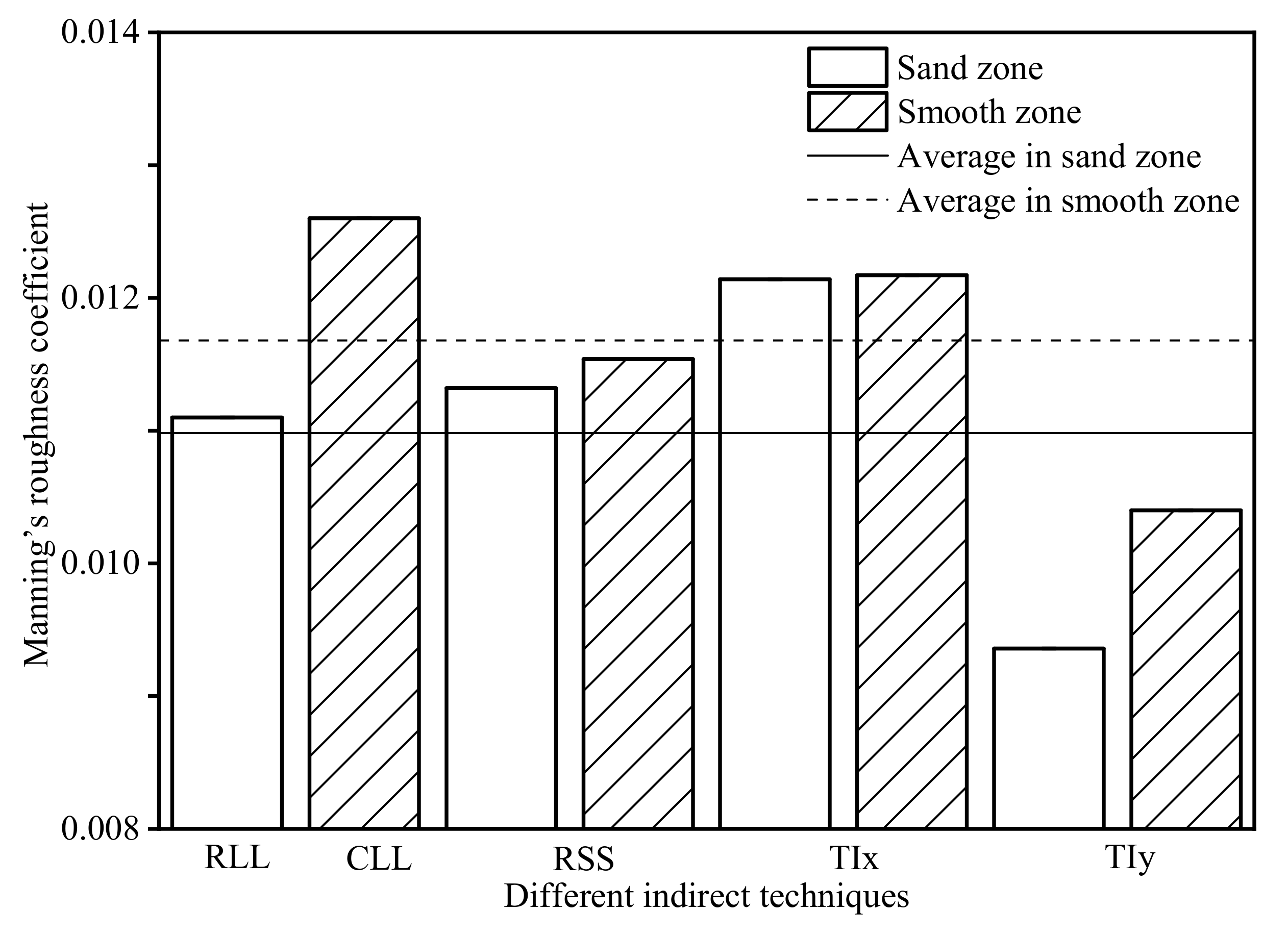
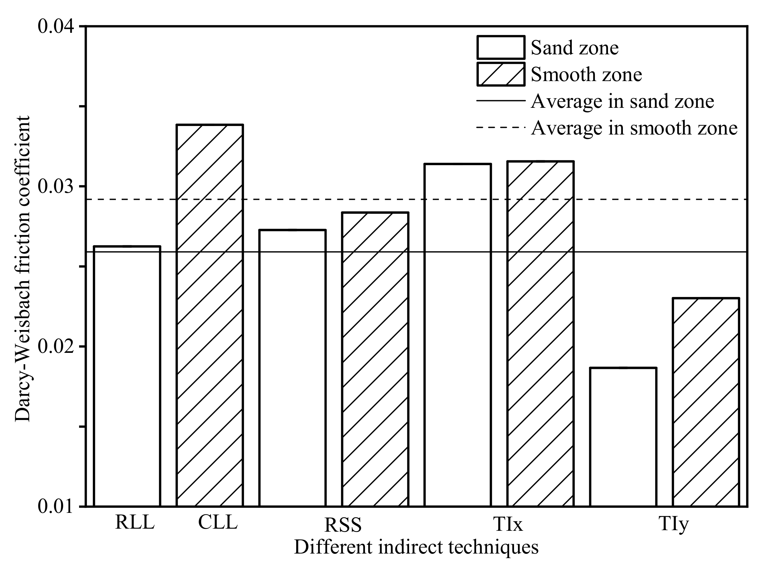
The Manning roughness coefficient, the Darcy–Weisbach friction coefficient and the equivalent grain roughness coefficient are considered as the resistance parameters in open channel flow hydraulics. The equivalent grain roughness coefficient is very suitable for the boundary condition in three-dimensional numerical simulations, although it is not easy to determine directly because of its wide variation in bed material size. The grain size distribution with different flow conditions may affect the estimation of the equivalent grain roughness coefficient [26]. Therefore, the Manning roughness coefficient, n, and the friction coefficient for the Darcy–Weisbach formula, f, were calculated from the critical shear velocity determined with each indirect method in both the sand zone and smooth zone. The Manning roughness coefficient and the friction coefficient for the Darcy–Weisbach formula, considering the depth averaged primary mean velocity, Um, and the water depth, d, can be calculated as follows:
The Manning roughness coefficients for the above-discussed indirect methods are denoted as and respectively. Similarly, the friction coefficients for the Darcy–Weisbach formula, estimated for the different indirect methods, are denoted as and respectively. The calculated values for the Manning roughness coefficient and the friction coefficient for the Darcy–Weisbach formula are listed in Table 6 for both the sand zone and smooth zone.
Figure 12 and Figure 13 show the Manning roughness coefficient and Darcy–Weisbach friction coefficient estimated by different methods in both zones.
Coefficients were calculated based on the estimated critical shear velocity which was found to be lower in the sand zone than in the smooth zone, as shown in Table 4. As a result, the Manning roughness and Darcy–Weisbach friction coefficients are higher in the smooth zone than in the sand zone, as shown in Figure 12 and Figure 13. However, the values between the two zones do not vary significantly. The flow is close to hydraulically smooth range for both zones; it might have influenced the determined roughness coefficients. Moreover, the Manning roughness coefficient value varies 0.009–0.013 for glass material [61]. It can be said that the calculated values for the Manning roughness coefficient agree well with the previous results.
Most of the available research determines incipient motion and bed shear stress in smooth beds or in rough beds separately. Moreover, available experimental and numerical studies discuss bed shear stress and turbulence statistics in detail in immobile bed condition. On the other hand, the present experimental study allows for limited mobile sand bed along its smooth acrylic bed. As a result, current experimental results elucidate the variations of bed shear stress, incipient motion and roughness coefficients on both types of beds. It should be noted that we cannot ignore uncertainties in fitting a logarithmic profile to velocity data in the present study. Furthermore, the velocity profile may not be logarithmic in complex flow fields.
4. Conclusions
An experimental investigation was conducted by constructing a closed conduit 10 cm in width, 5 cm in depth and 300 cm in length which was similar to EFA. A section of the conduit was made a sand zone with cohesionless sand particles and attached at the bottom of the conduit. By altering the flow rate in the conduit, the incipient motion was determined applying various indirect bed shear stress estimation methods in both the sand zone and the smooth zone. Two of the resistance characteristics, namely, the Manning roughness coefficient and the Darcy–Weisbach friction coefficient, were also evaluated during incipient motion at both zones. The results show that the bed shear stress estimated from methods based on the logarithmic flow profiles in both zones are relatively higher than those of the other methods. The dimensionless critical bed shear stress of incipient motion evaluated by these methods was found in good agreement with those of previous results in both the sand zone and the smooth zone. The Manning roughness and Darcy–Weisbach friction coefficients in the smooth zone were more than the corresponding values in the sand zone. However, these values showed a good agreement with available studies in both zones. The determined roughness coefficients produce helpful suggestions to express bed roughness condition for two- or three-dimensional numerical simulations for river flow and sediment transport. However, the size of the experimental closed conduit and its sediment bed is smaller than that used by other researchers. In the future, experiments focusing on bigger sized experimental facilities should be considered for a better understanding of the dynamics of incipient motion and roughness coefficient in both sand and smooth zones.
Author Contributions
Conceptualization, A.J.; methodology, A.J. and K.F.; laboratory analyses, A.J.; statistical analyses, A.J. and K.F.; writing—original draft preparation, A.J.; writing—review and editing, A.J., K.F. and A.M.; supervision, K.F. and A.M.; project administration, K.F. and A.M.; and funding acquisition, K.F. and A.M. All authors have read and agreed to the published version of the manuscript.
Funding
This work was funded by JSPS KAKENHI, Grant-in-Aid for Scientific Research (B), Grant Number 17H03889.
Institutional Review Board Statement
Not applicable.
Informed Consent Statement
Not applicable.
Data Availability Statement
The data supporting the findings of this study are available from the corresponding author upon reasonable request.
Acknowledgments
The first author thanks the Japanese Government for providing a MEXT scholarship. The authors also thank all the reviewers for their useful comments and suggestions.
Conflicts of Interest
The authors declare no conflict of interest.
References
- Pähtz, T.; Clark, A.H.; Valyrakis, M.; Durán, O. The Physics of Sediment Transport Initiation, Cessation, and Entrainment Across Aeolian and Fluvial Environments. Rev. Geophys. 2020, 58. [Google Scholar] [CrossRef]
- Safari, M.J.S.; Aksoy, H.; Unal, N.E.; Mohammadi, M. Experimental analysis of sediment incipient motion in rigid boundary open channels. Environ. Fluid Mech. 2017, 17, 1281–1298. [Google Scholar] [CrossRef]
- Vollmer, S.; Kleinhans, M.G. Predicting incipient motion, including the effect of turbulent pressure fluctuations in the bed. Water Resour. Res. 2007, 43. [Google Scholar] [CrossRef] [Green Version]
- Shields, A. Application of Similarity Principles and Turbulence Research to Bed-Load Movement; Ott, W.P.; Uchelen, J.C., Translators; California Institute of Technology: Pasadena, CA, USA, 1936. [Google Scholar]
- Briaud, J.L.; Ting, F.C.K.; Chen, H.C.; Cao, Y.; Han, S.W.; Kwak, K.W. Erosion Function Apparatus for Scour Rate Predictions. J. Geotech. Geoenviron. Eng. 2001, 127, 105–113. [Google Scholar] [CrossRef]
- Kang, G.-O.; Tsuchida, T.; Hashimoto, R.; Awazu, S.; Kim, Y.-S. Erosion resistance capacity of dredged marine clay treated with basic oxygen furnace slag. Soils Found. 2020. [Google Scholar] [CrossRef]
- Flack, K.A.; Schultz, M.P. Roughness effects on wall-bounded turbulent flows. Phys. Fluids 2014. [Google Scholar] [CrossRef] [Green Version]
- Cheng, N.-S.; Chiew, Y.-M. Incipient sediment motion with upward seepage. J. Hydraul. Res. 1999, 37, 665–681. [Google Scholar] [CrossRef]
- Southard, J.B.; Boguchwal, L.A. Bed configuration in steady unidirectional water flows; Part 2, Synthesis of flume data. J. Sediment. Res. 1990, 60, 658–679. [Google Scholar] [CrossRef]
- Costello, W.R.; Southard, J.B. Flume Experiments on Lower-Flow-Regime Bed Forms in Coarse Sand. SEPM J. Sediment. Res. 1981, 51, 849–864. [Google Scholar]
- Rees, A.I. Some Flume Experiments with A Fine Silt. Sedimentology 1966, 6, 209–240. [Google Scholar] [CrossRef]
- Ljunggren, P.; Sundborg, Ä. Some Aspects on Fluvial Sediments and Fluvial Morphology I. General Views and Graphic Methods. Geogr. Ann. Ser. A Phys. Geogr. 1967, 49, 333. [Google Scholar]
- Ashley, G.M. Classification of large-scale subaqueous bedforms; a new look at an old problem. J. Sediment. Res. 1990, 60, 160–172. [Google Scholar]
- Dyer, K.R. Coastal and Estuarine Sediment Dynamics; Wiley: Chichester, UK, 1986. [Google Scholar]
- Whitehouse, R.J.; Hardisty, J. Experimental assessment of two theories for the effect of bedslope on the threshold of bedload transport. Mar. Geol. 1988, 79, 135–139. [Google Scholar] [CrossRef]
- Chiew, Y.-M.; Parker, G. Incipient sediment motion on non-horizontal slopes. J. Hydraul. Res. 1994, 32, 649–660. [Google Scholar] [CrossRef]
- Parker, G.; Klingeman, P.C.; McLean, D.G. Bedload and size distribution in paved gravel-bed streams. J. Hydraul. Div. ASCE 1982. [Google Scholar] [CrossRef]
- Wilcock, P.R.; Southard, J.B. Experimental study of incipient motion in mixed-size sediment. Water Resour. Res. 1988, 24, 1137–1151. [Google Scholar] [CrossRef] [Green Version]
- Kuhnle, R.A. Incipient Motion of Sand-Gravel Sediment Mixtures. J. Hydraul. Eng. 1993, 119, 1400–1415. [Google Scholar] [CrossRef]
- Wilcock, P.R. Estimating Local Bed Shear Stress from Velocity Observations. Water Resour. Res. 1996, 32, 3361–3366. [Google Scholar] [CrossRef]
- Wei, T.; Schmidt, R.; McMurtry, P. Comment on the Clauser chart method for determining the friction velocity. Exp. Fluids 2005, 38, 695–699. [Google Scholar] [CrossRef]
- Kim, S.-C.; Friedrichs, C.T.; Maa, J.P.-Y.; Wright, L.D. Estimating Bottom Stress in Tidal Boundary Layer from Acoustic Doppler Velocimeter Data. J. Hydraul. Eng. 2000, 126, 399–406. [Google Scholar] [CrossRef] [Green Version]
- Nikora, V.; Goring, D. Flow turbulence over fixed and weakly mobile gravel beds. J. Hydraul. Eng. 2000. [Google Scholar] [CrossRef]
- Song, T.; Chiew, Y.M. Turbulence Measurement in Nonuniform Open-Channel Flow Using Acoustic Doppler Velocimeter (ADV). J. Eng. Mech. 2001, 127, 219–232. [Google Scholar] [CrossRef]
- Strom, K.B.; Papanicolaou, A.N. ADV Measurements around a Cluster Microform in a Shallow Mountain Stream. J. Hydraul. Eng. 2007, 133, 1379–1389. [Google Scholar] [CrossRef]
- Tominaga, A.; Sakaki, T. Evaluation of bed shear stress from velocity measurements in gravel-bed river with local non-uniformity. In Proceedings of the River Flow 2010: International Conference on Fluvial Hydraulics, Braunschweig, Germany, 8–10 September 2010; Bundesanstalt für Wasserbau: Karlsruhe, Germany, 2010. [Google Scholar]
- Al Faruque, M.A.; Balachandar, R. Seepage effects on turbulence characteristics in an open channel flow. Can. J. Civ. Eng. 2011, 38, 785–799. [Google Scholar]
- Balachandar, R.; Patel, V.C. Flow over a fixed rough dune. Can. J. Civ. Eng. 2008, 35, 511–520. [Google Scholar] [CrossRef]
- Cheng, N.S. Seepage effect on open-channel flow and incipient sediment motion. Ph.D. Thesis, Nanyang Technological University, Singapore, 1997. [Google Scholar]
- Hanmaiahgari, P.R.; Roussinova, V.; Balachandar, R. Turbulence characteristics of flow in an open channel with temporally varying mobile bedforms. J. Hydrol. Hydromech. 2017, 65, 35–48. [Google Scholar] [CrossRef] [Green Version]
- Robert, A.; Uhlman, W. An experimental study on the ripple-dune transition. Earth Surf. Process Landf. 2001. [Google Scholar] [CrossRef]
- Jewel, A.; Fujisawa, K.; Murakami, A. Effect of seepage flow on incipient motion of sand particles in a bed subjected to surface flow. J. Hydrol. 2019, 579. [Google Scholar] [CrossRef]
- Smart, G.M. Turbulent Velocity Profiles and Boundary Shear in Gravel Bed Rivers. J. Hydraul. Eng. 1999, 125, 106–116. [Google Scholar] [CrossRef]
- Roussinova, V.; Biswas, N.; Balachandar, R. Revisiting turbulence in smooth uniform open channel flow. J. Hydraul. Res. 2008, 46 (Suppl. 1), 36–48. [Google Scholar] [CrossRef]
- Dey, S.; Raikar, R.V. Characteristics of Loose Rough Boundary Streams at Near-Threshold. J. Hydraul. Eng. 2007, 133, 288–304. [Google Scholar] [CrossRef]
- Zanoun, E.-S.; Durst, F.; Nagib, H. Evaluating the law of the wall in two-dimensional fully developed turbulent channel flows. Phys. Fluids 2003, 15, 3079. [Google Scholar] [CrossRef]
- Cheng, N.S. Power-law index for velocity profiles in open channel flows. Adv. Water Resour. 2007, 30, 1775–1784. [Google Scholar] [CrossRef]
- Schultz, M.P.; Flack, K.A. The rough-wall turbulent boundary layer from the hydraulically smooth to the fully rough regime. J. Fluid Mech. 2007. [Google Scholar] [CrossRef] [Green Version]
- Nezu, I.; Nakagawa, H. (Eds.) Turbulence in Open-Channel Flows; IAHR Monographs; CRC Press/Balkema: Boca Raton, FL, USA, 1993. [Google Scholar]
- Fransson, J.H.M.; Matsubara, M.; Alfredsson, P.H. Transition induced by free-stream turbulence. J. Fluid Mech. 2005, 527, 1–25. [Google Scholar] [CrossRef]
- Hollingsworth, D.K.; Bourgogne, H.-A. The development of a turbulent boundary layer in high free-stream turbulence produced by a two-stream mixing layer. Exp. Therm. Fluid Sci. 1995, 11, 210–222. [Google Scholar] [CrossRef]
- Scheichl, B.; Kluwick, A.; Smith, F.T. Break-away separation for high turbulence intensity and large Reynolds number. J. Fluid Mech. 2011, 670, 260–300. [Google Scholar] [CrossRef] [Green Version]
- Degraaff, D.B.; Eaton, J.K. Reynolds-number scaling of the flat-plate turbulent boundary layer. J. Fluid Mech. 2000, 422, 319–346. [Google Scholar] [CrossRef]
- Miller, M.C.; Mccave, I.N.; Komar, P.D. Threshold of sediment motion under unidirectional currents. Sedimentology 1977, 24, 507–527. [Google Scholar] [CrossRef]
- Koster, E. Transverse Ribs: Their Characteristics, Origin and Paleohydraulic Significance. In Fluvial Sedimentology; Memoir 5; Miall, A.D., Ed.; Canadian Society of Petroleum Geologists: Calgary, AL, CA, 1978; pp. 161–186. [Google Scholar]
- Biron, P.M.; Robson, C.; Lapointe, M.F.; Gaskin, S.J. Comparing different methods of bed shear stress estimates in simple and complex flow fields. Earth Surf. Process Landf. 2004. [Google Scholar] [CrossRef]
- Julien, P.Y. Erosion and Sedimentation; Cambridge University Press: Cambridge, UK, 1998. [Google Scholar]
- Southard, J. Introduction to Fluid Motions and Sediment Transport; Massachusetts Institute of Technology: Cambridge, MA, USA, 2019. [Google Scholar]
- Mantz, P.A. Incipient transport of fine grains and flakes by fluids-extended Shields diagram. J. Hydraul. Div. 1977. [Google Scholar] [CrossRef]
- Yalin, M.S.; Karahan, E. Inception of sediment transport. J. Hydraul. Div. 1979. [Google Scholar] [CrossRef]
- Guo, J. Empirical model for Shields diagram and its applications. J. Hydraul. Eng. 2020, 146. [Google Scholar] [CrossRef]
- Kramer, H. Modellgeschiebe und Schleppkraft; Preuss. Versuchsanst. f. Wasserbau u. Schiffbau: Berlin, Germany, 1932; [In German]. [Google Scholar]
- Kramer, H. Sand mixtures and sand movement in fluvial models. Trans. Am. Soc. Civ. Eng. 1935, 100, 798–838. [Google Scholar] [CrossRef]
- Neill, C.R. Mean velocity criterion for scour of course uniform bed material. In Proceedings of the 12th Congress of the Int. Association for Hydraulic Research, 46–54 Fort Collins, CO, USA, 11–14 September 1967; International Association for Hydraulic Research: Madrid, Spain, 1967; Volume 3. [Google Scholar]
- USWES. Study of Riverbed Material and Their Use with Special Reference to the Lower Mississippi River; Mississippi River Commission Print: St. Louis, MO, USA, 1935. [Google Scholar]
- White, C.M. The equilibrium of grains on the bed of a stream. Proc. R. Soc. London 1940, 174, 322–338. [Google Scholar]
- Casey, H.J. About Bedload Movement. Ph.D. Thesis, Prussian Laboratory of Hydraulics and Shipbuilding, Technischen Hochschule, Berlin, Germany, 1935. [Google Scholar]
- Gilbert, G.K. The Transportaton of Debris by Running Water; US Government Printing Office: Washington, DC, USA, 1914. [Google Scholar]
- Grass, A. Initial Instability of Fine Bed Sand. J. Hydraul. Div. 1970. [Google Scholar] [CrossRef]
- Karahan, E. Initiation of motion for uniform and nonuniform materials. Ph.D. Thesis, Dept. of Civil Engineering, Istanbul Technical University, Istanbul, Turkey, 1975. [Google Scholar]
- Chow, V.T. Open-Channel Hydraulics; McGraw-Hill Book Co: New York, NY, USA, 1959. [Google Scholar]
Figure 1.
Experimental apparatus (not in scale).

Figure 2.
Velocity variations at different depths, y = 0.1h, y = 0.3h and y = 0.5h.

Figure 3.
Vertical distributions of primary mean velocity with log-law: (a) sand zone; and (b) smooth zone.
Figure 3.
Vertical distributions of primary mean velocity with log-law: (a) sand zone; and (b) smooth zone.


Figure 4.
Vertical distributions of Reynolds shear stress: (a) sand zone; and (b) smooth zone.


Figure 5.
Vertical distributions of turbulence intensities in x-direction: (a) sand zone; and (b) smooth zone.
Figure 5.
Vertical distributions of turbulence intensities in x-direction: (a) sand zone; and (b) smooth zone.

Figure 6.
Vertical distributions of turbulence intensities in y-direction: (a) sand zone; and (b) smooth zone.
Figure 6.
Vertical distributions of turbulence intensities in y-direction: (a) sand zone; and (b) smooth zone.

Figure 7.
Shear velocity estimated by different indirect methods: (a) sand zone; and (b) smooth zone.
Figure 7.
Shear velocity estimated by different indirect methods: (a) sand zone; and (b) smooth zone.

Figure 8.
Bed shear stress estimated by different indirect methods in the sand zone and smooth zone. The error bars represent the 95% confidence intervals (±two standard deviations).
Figure 8.
Bed shear stress estimated by different indirect methods in the sand zone and smooth zone. The error bars represent the 95% confidence intervals (±two standard deviations).

Figure 9.
Estimation of critical shear velocity from shear velocity calculated by different indirect methods at sand zone: (a) regression analysis of universal logarithmic law; (b) Reynolds shear stress; (c) turbulence intensity considering x-component of flow; and (d) turbulence intensity considering y-component of flow.

Figure 10.
Estimation of critical shear velocity from shear velocity calculated by different indirect methods at upstream edge of sand zone: (a) curve fitting to universal logarithmic law; (b) Reynolds shear stress; (c) turbulence intensity considering x-component of flow; and (d) turbulence intensity considering y-component of flow.


Figure 12.
The Manning roughness coefficient estimated by different indirect methods in the sand zone and smooth zone.
Figure 12.
The Manning roughness coefficient estimated by different indirect methods in the sand zone and smooth zone.

Figure 13.
The Darcy–Weisbach friction coefficient estimated by different indirect methods in the sand zone and smooth zone.
Figure 13.
The Darcy–Weisbach friction coefficient estimated by different indirect methods in the sand zone and smooth zone.


Table 1.
Experimental conditions.
| Flow Rate, Q lit/min | Reynolds Number, ReQ | Froude Number, Fr | Sediment Transport Rate, m3/s/m |
|---|---|---|---|
| 79 | 15,419 | 0.37600 | 1.188 × 10⁻⁸ |
| 80 | 16,028 | 0.38076 | 3.053 × 10⁻⁸ |
| 81 | 15,395 | 0.38552 | 3.296 × 10⁻⁸ |
| 83 | 16,199 | 0.39504 | 2.768 × 10⁻⁸ |
| 84 | 15,965 | 0.39980 | 4.551 × 10⁻⁸ |
| 86 | 16,346 | 0.40932 | 6.506 × 10⁻⁸ |
| 88 | 16,280 | 0.41883 | 2.229 × 10⁻⁷ |
| 89 | 16,916 | 0.42359 | 2.341 × 10⁻⁷ |
Table 2.
Streamwise flow velocity variations at specified depths.
| Streamwise Flow Velocity (m/s) at y = 0.1h | Streamwise Flow Velocity (m/s) at y = 0.3h | Streamwise Flow Velocity (m/s) at y = 0.5h | |||||||
|---|---|---|---|---|---|---|---|---|---|
| Q | Sand Zone | Smooth Zone | % Increase | Sand Zone | Smooth Zone | % Increase | Sand Zone | Smooth Zone | % Increase |
| 79 | 0.26551 | 0.27041 | 1.81262 | 0.31508 | 0.31384 | −0.39417 | 0.33174 | 0.33291 | 0.35159 |
| 80 | 0.26749 | 0.26908 | 0.59237 | 0.32124 | 0.32613 | 1.49949 | 0.34062 | 0.34212 | 0.43965 |
| 81 | 0.27569 | 0.28101 | 1.89063 | 0.32900 | 0.33291 | 1.17555 | 0.34084 | 0.34540 | 1.32219 |
| 83 | 0.28509 | 0.28829 | 1.11192 | 0.32967 | 0.33512 | 1.62635 | 0.34966 | 0.35272 | 0.86715 |
| 84 | 0.28174 | 0.28187 | 0.04605 | 0.33515 | 0.34073 | 1.63793 | 0.34877 | 0.35135 | 0.73566 |
| 86 | 0.28345 | 0.28691 | 1.20682 | 0.33945 | 0.34327 | 1.11349 | 0.35914 | 0.36232 | 0.87720 |
| 88 | 0.28540 | 0.29273 | 2.50730 | 0.34715 | 0.35344 | 1.77765 | 0.36852 | 0.37292 | 1.17770 |
| 89 | 0.30106 | 0.30128 | 0.07154 | 0.35669 | 0.35916 | 0.68581 | 0.36971 | 0.37168 | 0.53083 |
| Average | 0.28068 | 0.28395 | 0.33418 | 0.33807 | 0.35112 | 0.35393 | |||
| St. dev. | 0.01058 | 0.01014 | 0.01267 | 0.01360 | 0.01281 | 0.01327 | |||
Table 3.
Estimated shear velocity and bed shear stress by different indirect methods.
| Zone | Q (lit/min) | Shear Velocity (m/s) | Bed Shear Stress (pa) | ||||||
|---|---|---|---|---|---|---|---|---|---|
| Sand zone | 79 | 0.01583 | 0.01703 | 0.01701 | 0.01586 | 0.25059 | 0.29002 | 0.28934 | 0.25154 |
| 80 | 0.01845 | 0.01761 | 0.01755 | 0.01414 | 0.34040 | 0.31011 | 0.30800 | 0.19994 | |
| 81 | 0.01566 | 0.01638 | 0.01745 | 0.01477 | 0.24524 | 0.26830 | 0.30450 | 0.21815 | |
| 83 | 0.01652 | 0.01797 | 0.01812 | 0.01521 | 0.27291 | 0.32292 | 0.32833 | 0.23134 | |
| 84 | 0.01919 | 0.01809 | 0.01842 | 0.01393 | 0.36826 | 0.32725 | 0.33930 | 0.19404 | |
| 86 | 0.02034 | 0.01662 | 0.01871 | 0.01523 | 0.41372 | 0.27622 | 0.35006 | 0.23195 | |
| 88 | 0.02206 | 0.01612 | 0.01960 | 0.01501 | 0.48664 | 0.25985 | 0.38416 | 0.22530 | |
| 89 | 0.02214 | 0.01719 | 0.01910 | 0.01536 | 0.49018 | 0.29550 | 0.36481 | 0.23593 | |
| Average | 0.01877 | 0.01713 | 0.01825 | 0.01494 | 0.35849 | 0.29377 | 0.33356 | 0.22353 | |
| St. dev. | 0.00246 | 0.00068 | 0.00083 | 0.00060 | 0.09289 | 0.02335 | 0.03025 | 0.01778 | |
| Smooth zone | 79 | 0.01708 | 0.01703 | 0.01755 | 0.01446 | 0.29173 | 0.29002 | 0.30800 | 0.20909 |
| 80 | 0.01781 | 0.01680 | 0.01687 | 0.01545 | 0.31720 | 0.28224 | 0.28460 | 0.23870 | |
| 81 | 0.01802 | 0.01553 | 0.01667 | 0.01542 | 0.32472 | 0.24118 | 0.27789 | 0.23778 | |
| 83 | 0.01815 | 0.01590 | 0.01767 | 0.01531 | 0.32942 | 0.25281 | 0.31223 | 0.23440 | |
| 84 | 0.01831 | 0.01531 | 0.01787 | 0.01526 | 0.33526 | 0.23440 | 0.31934 | 0.23287 | |
| 86 | 0.01853 | 0.01810 | 0.01850 | 0.01617 | 0.34336 | 0.32761 | 0.34225 | 0.26147 | |
| 88 | 0.01872 | 0.01816 | 0.01950 | 0.01488 | 0.35044 | 0.32979 | 0.38025 | 0.22141 | |
| 89 | 0.01878 | 0.01830 | 0.01970 | 0.01630 | 0.35269 | 0.33489 | 0.38809 | 0.26569 | |
| Average | 0.01818 | 0.01689 | 0.01804 | 0.01541 | 0.33060 | 0.28662 | 0.32658 | 0.23768 | |
| St. dev. | 0.00052 | 0.00114 | 0.00105 | 0.00057 | 0.01868 | 0.03847 | 0.03816 | 0.01756 | |
Table 4.
Estimated critical shear velocity by different indirect methods.
| Zone | Critical Shear Velocity (m/s) | ||||
|---|---|---|---|---|---|
| Sand zone | 0.01599 | - | 0.01630 | 0.01749 | 0.01337 |
| Smooth zone | - | 0.01816 | 0.01662 | 0.01753 | 0.01497 |
Table 5.
Estimated dimensionless critical bed shear stress by different indirect methods.
| Zone | Dimensionless Critical Bed Shear Stress | ||||
|---|---|---|---|---|---|
| Sand zone | 0.02740 | - | 0.02847 | 0.03277 | 0.01949 |
| Smooth zone | - | 0.03533 | 0.02960 | 0.03294 | 0.02403 |
Table 6.
The estimated Manning roughness coefficient and friction coefficient for the Darcy–Weisbach formula considering different indirect methods.
Table 6.
The estimated Manning roughness coefficient and friction coefficient for the Darcy–Weisbach formula considering different indirect methods.
| Zone | Manning Roughness Coefficient | ||||
|---|---|---|---|---|---|
| Sand zone | 0.01110 | - | 0.01132 | 0.01214 | 0.00936 |
| Smooth zone | - | 0.01260 | 0.01154 | 0.01217 | 0.01040 |
| Friction Coefficient for Darcy–Weisbach Formula | |||||
| Sand zone | 0.02625 | - | 0.02727 | 0.03139 | 0.01867 |
| Smooth zone | - | 0.03384 | 0.02836 | 0.03155 | 0.02302 |
Publisher’s Note: MDPI stays neutral with regard to jurisdictional claims in published maps and institutional affiliations. |
© 2021 by the authors. Licensee MDPI, Basel, Switzerland. This article is an open access article distributed under the terms and conditions of the Creative Commons Attribution (CC BY) license (https://creativecommons.org/licenses/by/4.0/).
Share and Cite
MDPI and ACS Style
Jewel, A.; Fujisawa, K.; Murakami, A. Evaluation of Incipient Motion of Sand Particles by Different Indirect Methods in Erosion Function Apparatus. Water 2021, 13, 1118. https://doi.org/10.3390/w13081118
AMA Style
Jewel A, Fujisawa K, Murakami A. Evaluation of Incipient Motion of Sand Particles by Different Indirect Methods in Erosion Function Apparatus. Water. 2021; 13(8):1118. https://doi.org/10.3390/w13081118
Chicago/Turabian StyleJewel, Arif, Kazunori Fujisawa, and Akira Murakami. 2021. "Evaluation of Incipient Motion of Sand Particles by Different Indirect Methods in Erosion Function Apparatus" Water 13, no. 8: 1118. https://doi.org/10.3390/w13081118
Note that from the first issue of 2016, this journal uses article numbers instead of page numbers. See further details here.