
Assessing the Hydroclimatic Movement under Future Scenarios Including both Climate and Land Use Changes


1
Department of Rural Systems Engineering, Seoul National University, Seoul 08826, Korea
2
Graduate School of International Agricultural Technology & Institutes of Green Bio Science and Technology, Seoul National University, Pyeongchang 25354, Korea
3
Research Institute of Agriculture and Life Sciences, Seoul National University, Seoul 08826, Korea
4
Department of Rural Systems Engineering, Research Institute for Agriculture and Life Sciences, Institutes of Green Bio Science and Technology, Seoul National University, Seoul 08826, Korea
*
Author to whom correspondence should be addressed.
Water 2021, 13(8), 1120; https://doi.org/10.3390/w13081120
Submission received: 12 April 2021
/
Revised: 12 April 2021
/
Accepted: 14 April 2021
/
Published: 19 April 2021
(This article belongs to the Special Issue Climate Change Impacts on Hydrological Processes and Water Resources of Local Watersheds)
Abstract
:In this study we simulated the watershed response according to future climate and land use change scenarios through a hydrological model and predicting future hydroclimate changes by applying the Budyko framework. Future climate change scenarios were derived from the UK Earth system model (UKESM1), and future land use changes were predicted using the future land use simulation (FLUS) model. To understand the overall trend of hydroclimatic conditions, the movements in Budyko space were represented as wind rose plots. Moreover, the impacts of climate and land use changes were separated, and the watersheds’ hydroclimatic conditions were classified into five groups. In future scenarios, both increase and decrease of aridity index were observed depending on the watershed, and land use change generally led to a decrease in the evaporation index. The results indicate that as hydroclimatic movement groups are more diversely distributed by region in future periods, regional adaptation strategies could be required to reduce hydroclimatic changes in each region. The results derived from this study can be used as basic data to establish an appropriate water resource management plan and the governments’ land use plan. As an extension of this study, we can consider more diverse land use characteristics and other global climate model (GCMs) in future papers.
1. Introduction
According to the World Urbanization Prospects [1], more people live in urban areas than in rural areas globally, with 55% of the world’s population residing in urban areas in 2018; by 2050, this proportion is projected to increase to 68%. Urbanization leads to urban development demand, resulting in an increase in impervious surface areas. Increased imperviousness causes flooding of rivers, deterioration of water quality in watersheds during floods, and deficit of stored water during drought. It also causes changes in the urban ecosystem, such as reducing the habitat of plants, leading, in turn, to disturbances in the water circulation system [2,3,4].
Along with the increase in watershed impermeability due to human activities, the watershed hydrologic condition is also significantly affected by climate change. The Intergovernmental Panel on Climate Change (IPCC) reports that compared to pre-industrial times, several regional changes in climate are evaluated to occur with an increase in global warming by up to 1.5°C, including warming in many regions [5]. Owing to these changes in climatic conditions, the frequencies and intensities of some extreme weather and climate events have increased as a consequence of global warming and are expected to increase continuously under medium- and high-emission scenarios [6]. Furthermore, elevated atmospheric CO2 concentration and climate change influence the hydrological circulation by affecting the spatio-temporal distribution of rain, atmospheric temperature, evapotranspiration, and vegetation [7,8,9,10,11,12]. Several studies based on modeling and observational data imply that global climate changes will affect watershed hydrology, including runoff and pollutant behavior [9,11,12,13].
Such changes in the watershed hydrologic system due to human impacts and climate changes result in various environmental changes in the region [14]. Currently, because of the changes in the hydrological system, various water-related problems, such as an increase in peak flow during torrential rains, depletion of groundwater, dryness of rivers, and pollution of rivers by non-point pollutants occur [15,16]. Furthermore, in the future climate change environments, these problems can also affect the atmospheric environment and cause urban heat island and tropical night phenomena [17]. Therefore, to cope with these problems, numerous countries worldwide are establishing various measures pertaining to watershed management, such as the development of rainwater discharge reduction systems to improve the water circulation system [18,19,20]. However, to devise appropriate measures to improve the water circulation system and establish long-term plans, predicting the changes in hydrological conditions due to climate and land use changes and quantitatively identifying the impact of each on the hydrological conditions become necessary.
The methods employed for the prediction of future hydrological changes can be divided into the following: using past observational data; using climate forecast models; and the application of climate models to deterministic hydrologic models [21,22]. The limitation of the first method is that it does not consider the uncertainty of the future climate, and the disadvantage of the second method is that it does not sufficiently consider the regional variability of hydroclimatic characteristics. Therefore, the third method is used in many studies as it allows the uncertainty of future climate, regional characteristics, and complex hydrological mechanisms to be considered [12,23,24]. In addition, several researchers have analyzed the effects of human activities and climate change on watershed by applying land use changes to the watershed models [23,25,26,27,28,29].
Meanwhile, if only the hydrological model is applied, it is possible to simulate changes in individual hydrologic parameters such as runoff and evapotranspiration, but there is a limit to grasp the overall hydroclimatic shifts of the watershed. One effective way for comprehensively assessing the complex hydroclimatic condition of a watershed is through the Budyko framework [30], which can describe the watershed hydrological condition shifts over time through a combination of aridity and evaporation indices [31,32]. In particular, several studies have evaluated watershed hydroclimatic changes through the direction and magnitude of movements in the Budyko space [31,32,33,34,35,36]. Meanwhile, due to interactive effects of climate change and land use shifts, efforts have been made to separate and quantify the effects of climate change and human activity on runoff based on the Budyko equations which consider water and energy limitations in the long-term hydrological processes [29,37,38,39]. However, in most such studies, the input factors of the Budyko framework were based on observational data, and future changes were predicted based on the past climate change and land use changes to date [27,37,38,39,40]. Although several studies have used future climate change scenarios, there is a lack of research that predicts future hydroclimatic changes by considering changes in land use. For this reason, the uncertainty of future climate or land use changes and complicated hydrologic mechanisms cannot be taken in account, which is a limitation.
To assess the future hydroclimatic changes, it is necessary to apply future climate and land use change scenarios to a hydrological model to obtain predicted values of each hydrological parameter and apply them to the Budyko framework to comprehensively analyze changes in hydroclimatic conditions. Therefore, the aims of this study are: (1) to develop the future climate and land use change scenarios; (2) to apply hydrologic model with current and future conditions; (3) to analyze the changes in hydroclimatic conditions using Budyko framework; and (4) to quantitatively identify the impacts of climate and land use changes.
2. Materials and Methods
2.1. Study Area
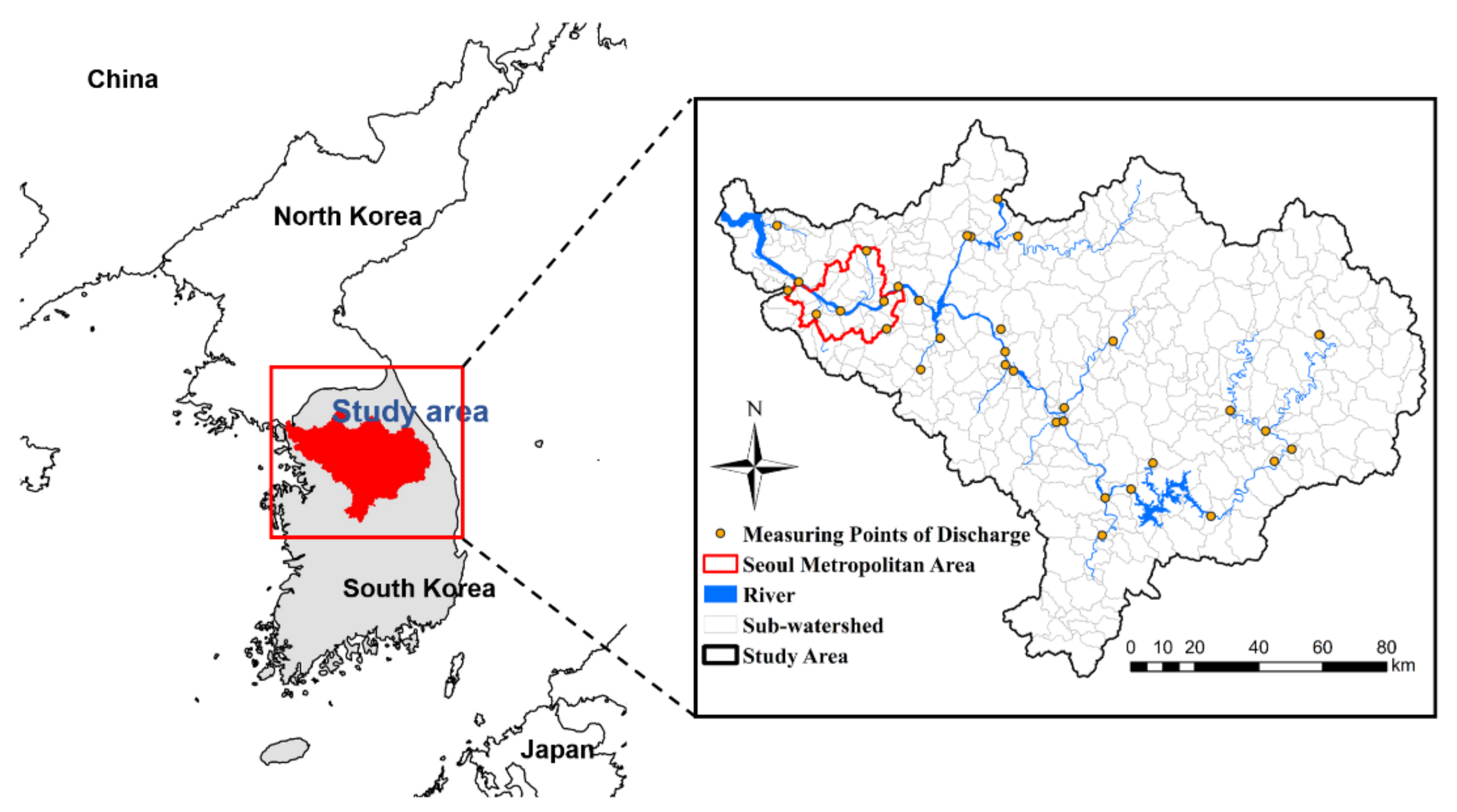
The Han River Basin (HRB), which is situated in the central part of the Korean Peninsula (37°44′60′’N, 126°10′60′’E), was selected as the target area (Figure 1). The area of the HRB is 26,219 km2, making it the largest river basin in Korea, and the associated river, which is 5417 km in length, comprises of two major distributary channels; the North Han River (NHR) which has an area of 10,652 km2 and South Han River (SHR) with an area of 12,514 km2 [41]. In this study, a total area of 18,220 km2 including 154 watersheds was considered; part of the NHR where data acquisition is restricted was excluded. The average annual precipitation in this area is approximately 1300 mm, and 70% of it is concentrated during the summer season (late June to mid-July) [42]. As the surface runoff is heavily dependent on precipitation during the monsoon season, it has an important effect on water resources in the HRB. Furthermore, more than 20 million people live in the HRB, including the Seoul metropolitan area with a population of approximately 10 million, and the NHR and SHR serve as their major sources of drinking water [43].
Seoul is located in the western part of the HRB; its development as a city started in the late 1960s and currently it occupies most of the urban area in the HRB. In addition, as demand for land development continues to rise in the suburban areas in Seoul, the built-up area is expected to expand. Since urbanization causes an increase in impervious surfaces, it could alter the water circulation in the basin.
2.2. Land Use and Land Cover Change (LUCC) Simulation
In this study, the future land use change was simulated to analyze the hydrological effect of the increase in impervious surface due to human activities. The cellular automata (CA)-based future land use simulation (FLUS) model was used to simulate urban growth in the study area. The FLUS model has been employed to simulate complex land use changes on a global scale [44]. Furthermore, its superiority has been demonstrated over other existing multiple land use and land cover change (LUCC) simulation models, such as the traditional conversion of land use and its effects at small regional extent (CLUE-S) model, and Logistic-CA model [45].
2.2.1. FLUS Model
The FLUS model can be implemented by the process of generating the probability of occurrence (PoO) surface through training an artificial neural network (ANN) model and performing spatial simulation based on a CA model [46]. The ANN is used for considering both natural ecological effects and influence of human activities by determining relationships between historical land cover and the diverse driving factors. The ANN was composed of prediction and training stages, which are described as follows.
The PoO surfaces estimated from the ANN are used to guide the placement of land use type distribution changes, and a self-adaptive inertia coefficient is employed to adjust the total probability of each land cover grid [46]. The self-adaptive inertia and competition mechanism were designed to handle the interactions among different land use types, which improved the capability to overcome uncertainty and randomness of land use change [45,47].
The model simulation is divided into several intervals. The ‘bottom-up’ CA model and the ‘top-down’ land use demand prediction model are tightly coupled to each other [46]. As a future land use demand forecasting model, the Markov chain model which predicts land use demand by determining the possibility of conversion from one category to another during the two data acquisition period was used [48]. It has been successfully employed in several studies because of its ability to quantify not only the conversion states between land use and land cover (LULC) types, but also the rate of conversion among each type [49,50].
2.2.2. Data Processing
For ANN-based PoO estimation, the land use maps for the coverage areas in 1975 and 2013 were used. These maps were divided into seven classes: built-up land, agricultural land, forest land, grassland, wetland, barren land, and water. In addition, four spatial data types such as the digital elevation model (DEM), slope, aspect, and distance to rivers were used as the driving factors. The data used in FLUS model are listed in Table 1.
The Markov model was applied to the study area from 2013 to 2051 and 2089 by using the probability transition matrix and transition maps of one class to another class from 1975 to 2013. Land demand pixel changes calculated as a result of the Markov model are as shown in Table 2.
2.3. Climate Data
In this study, historical meteorological data and future climate projections from the global climate model (GCM) were used to investigate the runoff for climate change. Daily climate variables, including rainfall, maximum, minimum, and mean temperatures, wind speed, relative humidity, and sunshine hours collected from a total of 27 meteorological stations from 1970–2015 were obtained from the Korea Meteorological Administration. For the next phase of the study, to predict the future hydrological changes of the basin, climate change data were derived from the UK Earth system model (UKESM1), which is the GCM of the Coupled Model Intercomparison Project Phase 6 (CMIP6). UKESM1 was selected as it exhibits a higher probability of precipitation in HRB than that of other CMIP6 models, which could be used to simulate extreme hydrologic conditions in the future. There are five shared socioeconomic pathways (SSPs) that consider adaptation to climate change and social capabilities to reduce greenhouse gas emissions till 2100. In this study, future GCM climate data were extracted under two future scenarios, namely SSP2–4.5, which is a medium forcing scenario, and SSP5–8.5, which is a strong forcing scenario. In addition, bias correction/spatial downscaling method was applied to remove bias and statistically downscale the projected weather data using historical (1976–2005) climate data from each meteorological station.
2.4. HSPF Model
The hydrology of the HRB was modeled with Hydrological Simulation Program—Fortran (HSPF), which is a comprehensive process-based watershed model which can be employed to simulate watershed runoff and water quality over a long time and a wide range of watershed sizes and conditions [51]. It allows the user to create various scenarios by adjusting land use types and climate factors [51]. HSPF employs lumped parameter segments, and the watershed is segmented into sub-watersheds having homogeneous characteristics throughout [52]. Three main modules that represent the major watershed processes exist. The PERLND (pervious land segment) module deals with pervious land, and IMPLND (the impervious land segment) module is used for impervious surfaces. The RCHRES (free-flowing reach or mixed reservoirs) module models water bodies like streams or reservoirs [53]. In this study, HSPF was developed for the 154 sub-watersheds in the HRB at a daily time step to simulate streamflow, and the study was carried out in two parts. First, past (1970–2015) hydrologic conditions of the watershed were simulated and the model was calibrated for the period of 2010–2014. Secondly, future climate and land use conditions were applied to simulate future changes of the watershed for the period of 2045–2099.
2.4.1. HSPF Input
A past (as of the year 1975) land use map from the water resources management information system (WAMIS) of the Ministry of Environment in Korea, and current (as of the year 2013) land use map from the National Geographic Information Institute (NGII) of the Ministry of Land, Infrastructure and Transport in Korea were obtained as land use data. In addition, as a result of the FLUS model simulation, the land use maps of 2051 and 2089 were used as the land use data for future period simulations. A 1:5000 DEM was obtained from the NGII. As meteorological station data, past (1970–2015) and future (2045–2099) daily precipitation, temperature, average wind speed, average humidity, and average solar radiation data of 27 meteorological stations were used. Finally, stream flow quantity data from water environment information system of the Ministry of Environment in Korea and dam releases data from WAMIS were obtained for the periods of 2004–2015 and 2006–2015, respectively.
2.4.2. Model Calibration
The HSPF model was calibrated for daily runoff of 2010–2012 by adjusting the five streamflow related parameters, INFLILT (the infiltration capacity index), FOREST (pervious land fraction covered by forest), SLSUR (slope of the overland flow plane), LSUR (length of the overland flow plane), and INTFW (interflow inflow parameter). The values of each parameter were determined using soil data, land use, and slope, and adjusted through a trial-and-error method to appropriately fit the modeled and observed data. A soil map that applied the four soil group classification methods proposed in 2007 by the National Institute of Agricultural Sciences and Technology was used for soil data. The INFILT parameter, which is one of the most sensitive parameters to modeled streamflow, was calculated considering the spatial distribution of the hydrologic soil groups and the minimum value of the penetration rate for each hydrologic soil groups. SLSUR and LSUR were estimated by calculating the flow length and slope from the DEM, respectively, and FOREST was calculated using the forest ratio of each watershed unit. The INTFW parameter value was determined as a value applicable to all subwatersheds, land use, and soils by referring to Diaz-Ramirez et al. [54]. The calibrated values for each parameter are given in Table 3.
The model was validated using data of 2013–2014. To verify the accuracy of model simulation, three main statistical methods proposed by Moriasi et al. [55] were used to quantitatively compare modeled and observed streamflow data: the coefficient of determination (R2), Nash-Sutcliffe coefficient of efficiency (NSE), and percent bias (PBIAS). Based on general performance ratings for recommended statistics proposed by Moriasi et al. [55], the model is found to have a satisfactory performance if R2 > 0.60, NSE > 0.50, and PBIAS ≤ ± 15% for watershed-scale models [55].
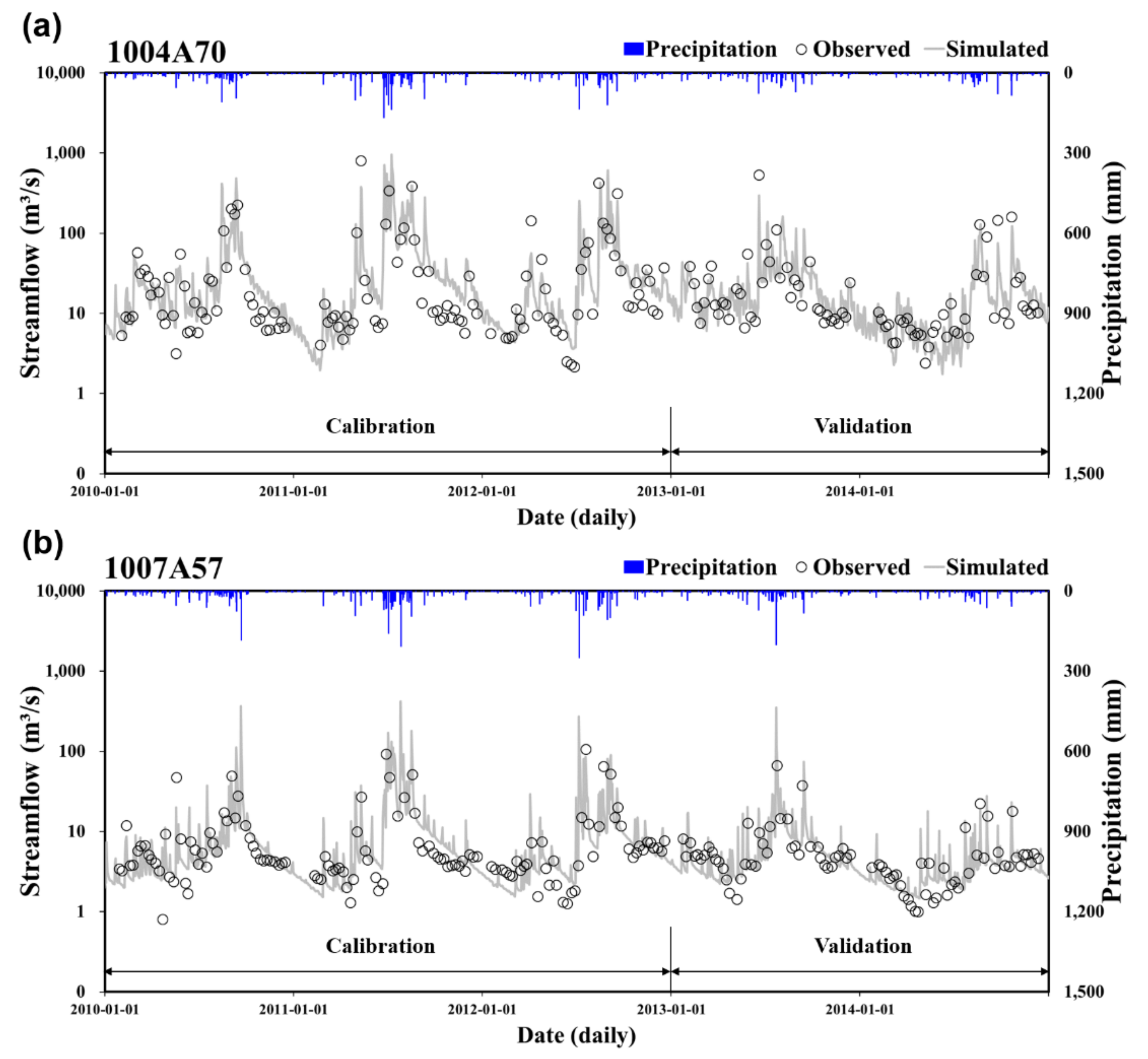
The results of hydrologic calibration and validation of the 30 unit watersheds in HRB are shown in Table 4 and observed and simulated streamflow for some unit watersheds during the calibration and validation periods are shown in Figure 2. Some unit watersheds with R2 close to 1 were found to be directly affected by dam discharge as they are adjacent to the dam. Although PBIAS could not meet the satisfactory criteria in some unit watersheds by overestimating the streamflow under high flow conditions, most of the unit watersheds met the criteria of R2, NSE, and PBIAS; thus, it can be stated that the model performs satisfactorily in simulating watershed streamflow.
2.5. Assessment of Hydrological Condition of Watershed Based on Budyko Framework
2.5.1. Budyko Framework
The Budyko framework is a widely used representation of the land water balance that describes the partitioning of mean annual precipitation into streamflow and evaporation as a function of the ratio of the atmospheric water supply to water demand [56]. Budyko framework originated from the assumption that precipitation in long-term temporal scales is divided into evaporation and runoff.
Budyko [57] demonstrated that the evaporation ratio, E/P, in a watershed over a long-term time scale can be expressed as follows:
where is the ratio of potential evapotranspiration to precipitation, i.e., Ep/P.
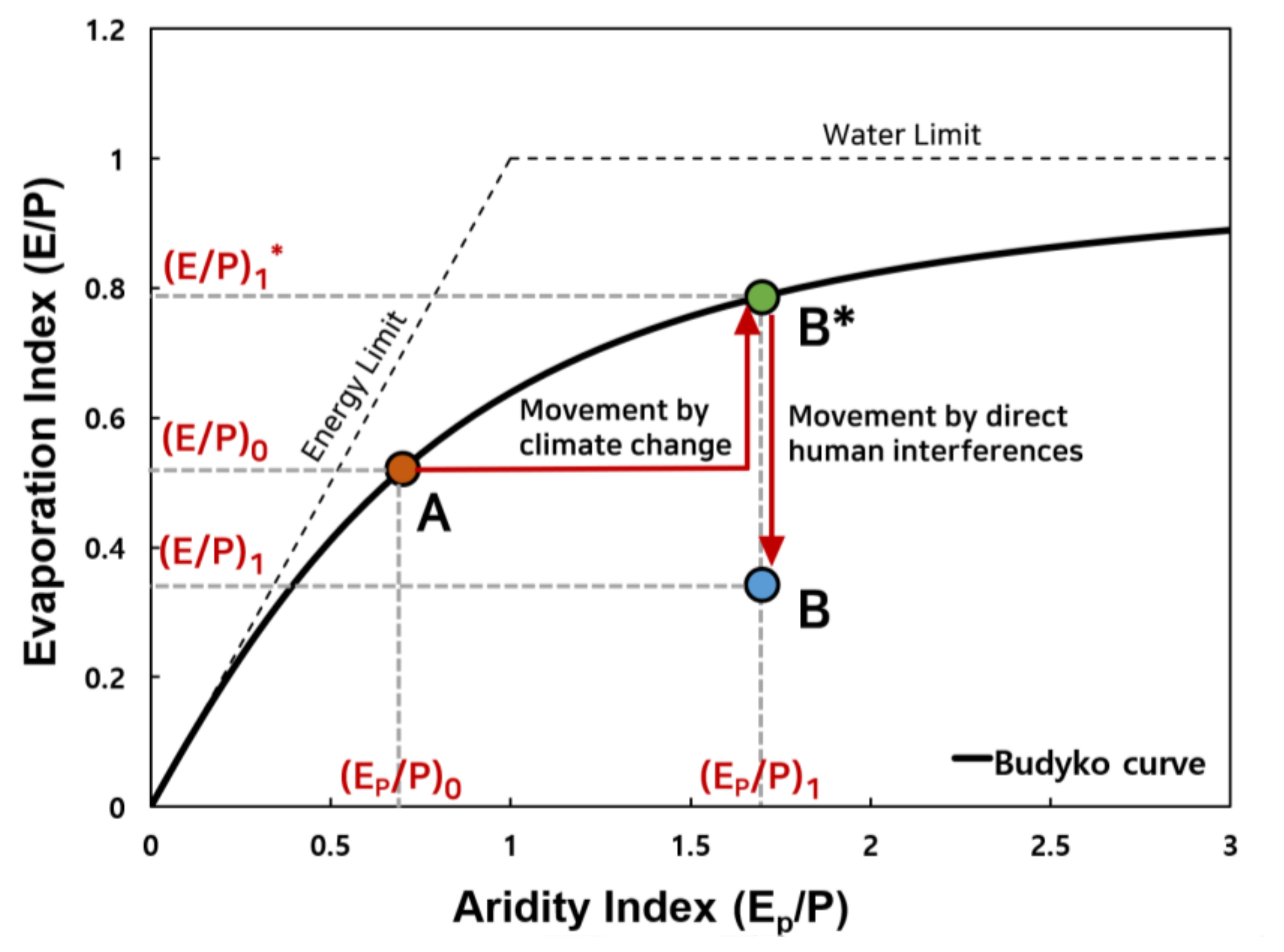
Based on the assumptions of the water and energy balance in the annual time unit, the Budyko framework was designed to describe the annual hydrological cycle and climate characteristics using the evaporation and aridity indices, which are the ratios of the annual actual and potential evapotranspiration to precipitation, respectively. The relationship between these two indices is represented by Budyko–type curves, which express the evaporation index in terms of the aridity index as shown in Figure 3. Budyko [57] set the limits for curves by assuming two types of watershed conditions limited by energy supply and water supply. For watersheds with an aridity index less than 1, the energy supply is the limiting factor for evapotranspiration, while for watersheds with an aridity index larger than 1, the water supply is the limiting factor [37]. If hydroclimatic changes occur, the watershed changes from state A to B. In the case where only the climate change effects are affected, the evaporation index also changes according to the change of aridity index, and the watershed in state A moves to a different point on the same Budyko curve, B*. However, in reality, other factors besides climate change, such as vegetation type [58], soil properties [59], and topography [60] also affect the evaporation index, and the watershed can be located at a new point B away from the initial Budyko curve.
As the Budyko curve was developed mainly using European data, other numerous equations have been proposed to improve regional estimates and to account for various land cover types [38,61,62,63,64,65,66]. One of the most popular forms is the one proposed by Fu [63]; a rational function equation where the single parameter, ω, in the equation can be calibrated against local data as [38]:
In this study, the runoff and potential evaporation of past period (1970–1984) derived from the HSPF simulation was applied to the equation of Fu, and the parameter ω was calculated for each watershed with the objective function as the root-mean-square error.
2.5.2. Hydroclimatic Change in the Budyko Space
Van der Velde et al. [33] described the changes on the Budyko curve over time due to the change of hydroclimatic condition as a vector with direction of movement and magnitude, which has been utilized in many studies [31,32,34,35,36,67,68]. The direction indicates how the evaporation and aridity indices change, while the magnitude refers to the degree of sensitivity of the watershed to climate change.
The direction (D) of movement and magnitude (M) can be calculated as follows:
where b = 90° when > 0 and b = 270° when < 0.
In this study, using the same approach, we represented the movements on Budyko space for 154 watersheds as wind roses of direction and magnitude. A wind rose plot shows the regional distribution of direction and magnitude of change and is advantageous of being able to simply identify the overall trend of movement in large sets of watersheds.
2.5.3. Separation of the Impact of Climate and Land Use Changes on Hydrological Condition
As the movement along the vertical direction in the Budyko space can be driven by both climate change and direct human impacts, the effects of each should be distinguished. As we considered land use change as a factor of direct human activity, we separated the change in the evaporation index into the change caused by land use change (Δ(E/P)l) and change caused by climate change (Δ(E/P)C). They were calculated as follows:
Δ(E/P)l = (E/P)1 − (E/P)1*
Δ(E/P)c = (E/P)1* − (E/P)0,
Furthermore, to separate the impact of climate and land use changes on mean annual streamflow, we calculated the magnitude of land use induced change of streamflow(ΔQl) and climate induced change of streamflow(ΔQc) using the decomposition method of [37]:
ΔQl = [(E/P)1−(E/P)1*] P1
ΔQc = ΔQ−ΔQl
ΔQ = Q1−Q0
For comparing the values of ΔQl and ΔQc among watersheds, percentage changes of climate and land use induced runoff relative to initial period runoff were calculated as follows [37]:
ΔQc% = 100(ΔQc÷Q1)
ΔQl% = 100(ΔQl÷Q1)
3. Results and Discussion
3.1. FLUS Model Implementation Result
For the PoO estimation, land use data and four spatial driving factors (DEM, aspect, slope, and distance from rivers) were used to calibrate the ANN model. We set the ANN model to consist of four neurons in the input layer corresponding to the number of spatial elements, 12 neurons in the hidden layers, and seven neurons in the output layer corresponding to the number of land use types. As the training dataset, 0.1% of the total pixels across the entire area were randomly selected.
The model simulation can be divided into two steps: model validation and scenario simulation. The model validation was conducted from 1975 to 2013, while the scenario simulation was applied from 2013 to 2051 and to 2089. For the simulation result validation, the ‘figure of merit’ (FoM) indicator was used to reflect cell-level and pattern-level agreement [46], and Kappa coefficient and overall accuracy were also calculated.
3.1.1. Simulation from 1975–2013
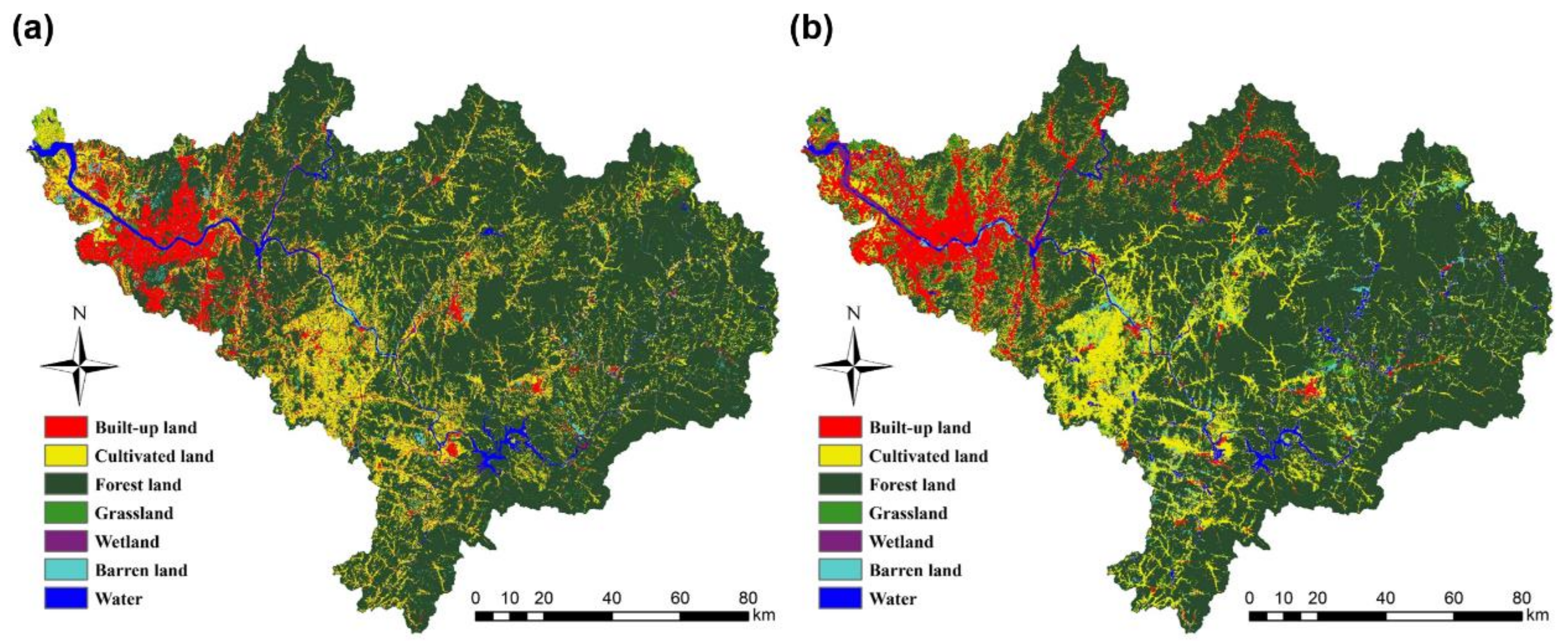
According to the ANN prediction process, PoO surfaces were generated, and based on them we simulated land use change from 1975 to 2013. In the CA model-based spatial simulation process, actual land use demand in 2013 was used as a top-down effect which helps improve simulation accuracy [45]. Figure 4 shows the actual and simulated land use in 2013, and a high correlation is seen between the two patterns.
To quantitatively evaluate the simulated result accuracy, confusion matrix of the simulated result versus the actual land use was calculated (Table 5), and from here, the Cohen’s Kappa coefficient and the overall accuracy were calculated as 0.47 and 0.73, respectively. Furthermore, the simulation result was also validated using the FoM indicator which avoids overestimation of the accuracy in traditional validation methods [69,70,71]. The FoM indicator can be expressed as follows:
where A is the area of error due to observed change predicted as persistence, B is the area of accuracy due to observed change predicted as change, C is the area of error due to observed change predicted as changing to an incorrect category, and D is the area of error due to observed persistence predicted as change.
Previous studies have demonstrated that FoM commonly ranges from 10%–30% for existing land use change models; the FoM value of 0.1619 here is either equal or greater than those in other studies of land use change simulation [44,46,71,72]. Thus, the performance of our model is reliable, and driving factors and parameters are applicable to predicting future land use changes.
3.1.2. Scenario Simulation
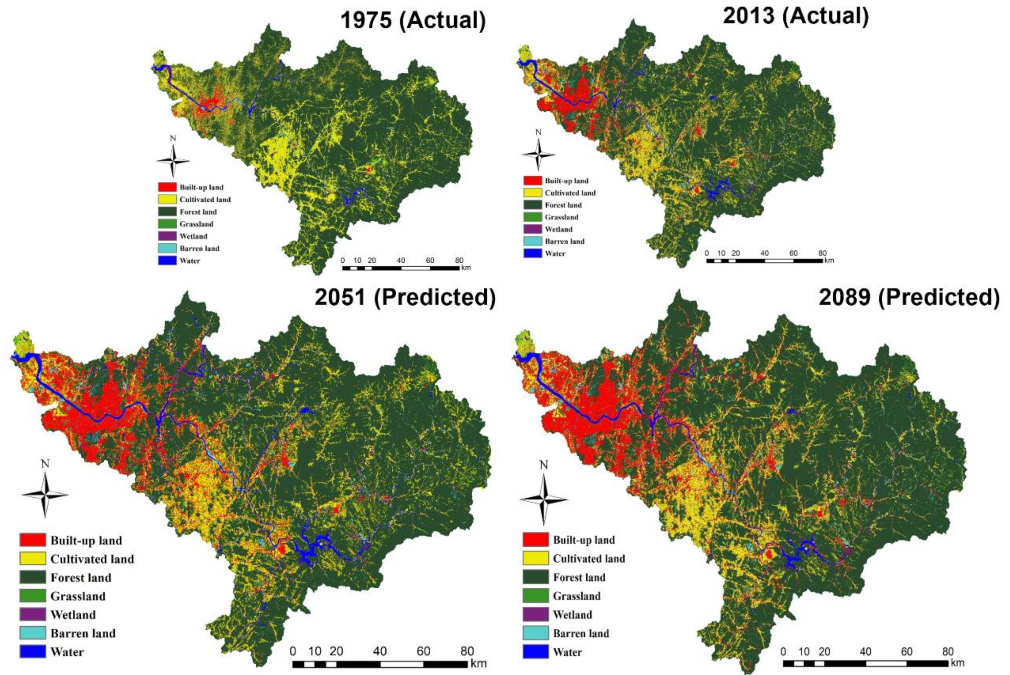
For the future land use change simulation, future land use demand in each type was determined by the Markov chain, and we used the multiple CA model to simulate the spatial land use change dynamics from 2013–2051 and 2089. The simulation results are shown in Figure 5. The land use maps (Figure 5) and area change in each land use type (Table 6) indicates that the change is mainly characterized by the expansion of built-up land and loss of cultivated and forest lands. Built-up land, which accounted for 1.55% of the total area in 1975 and 6.95% in 2013, was forecast to increase to 10.3% in 2051 and 12.4% in 2089. Agricultural areas were expected to decline from 20.99% in 1975 and 15.67% in 2013 to 14.40% in 2051 and 13.99% in 2089. Forest areas accounted for 73.49% in 1975 and 68.52% in 2013 and were forecast to decline to 64.83% in 2051 and 64.27% in 2089. Compared to the actual land use pattern in 2013, with the passage of time, built-up land is expected to expand primarily in metropolitan areas, with many of the current agricultural areas being replaced by built-up areas.
3.2. Projection of Future Climate Change
In this study, the future period was divided into near future (NF, 2045–2064) and the far future (FF, 2080–2099), and it was assumed that the land use in each period is the same as that in the 2051 and 2089 predictions in Section 3.1.
Table 7 shows the summarized results of annual precipitation and annual mean temperature for the past period (1970–1984; also set as the base period), current period (1996–2015), NF (2045–2064), and FF (2080–2099) under two shared socioeconomic pathways (SSPs, SSP2 and SSP5). For the current period, the annual precipitation and annual mean temperature were increased by about 24.19% and 2.05%, respectively, from the past period. In the SSP2 scenario, the annual precipitation was predicted to increase by 31.59% and 53.57%, respectively, in the NF and FF periods from the base period. The annual mean temperature was predicted to increase by 32.48% and 49.39% respectively. In the SSP5 scenario, the annual precipitation was projected to increase by 29.81% and 63.27%, respectively, during the NF and FF periods, and the annual mean temperature was forecasted to increase by 45.54% and 79.84%, respectively. Thus, in both scenarios, both the annual rainfall and annual mean temperature are expected to increase further into future. During the NF period, the mean annual precipitation was slightly larger in SSP2 scenario, but the difference between the maximum and minimum values of the annual precipitation was slightly larger in the SSP5 scenario. Meanwhile, during the FF period, the annual precipitation value was much larger in the SSP5 scenario. In addition, as the projected range of annual total rainfall increases in FF, it is indicated that the uncertainty range increases in FF more than in NF. The average annual mean temperature was predicted to be higher in SSP5 than in SSP2 in both NF and FF periods due to climate change.
3.3. Simulated Hydrologic Components for Future Scenarios
The HSPF model was used to simulate the annual streamflow and annual potential evapotranspiration of each watershed by applying climate and land use data for current and future periods.
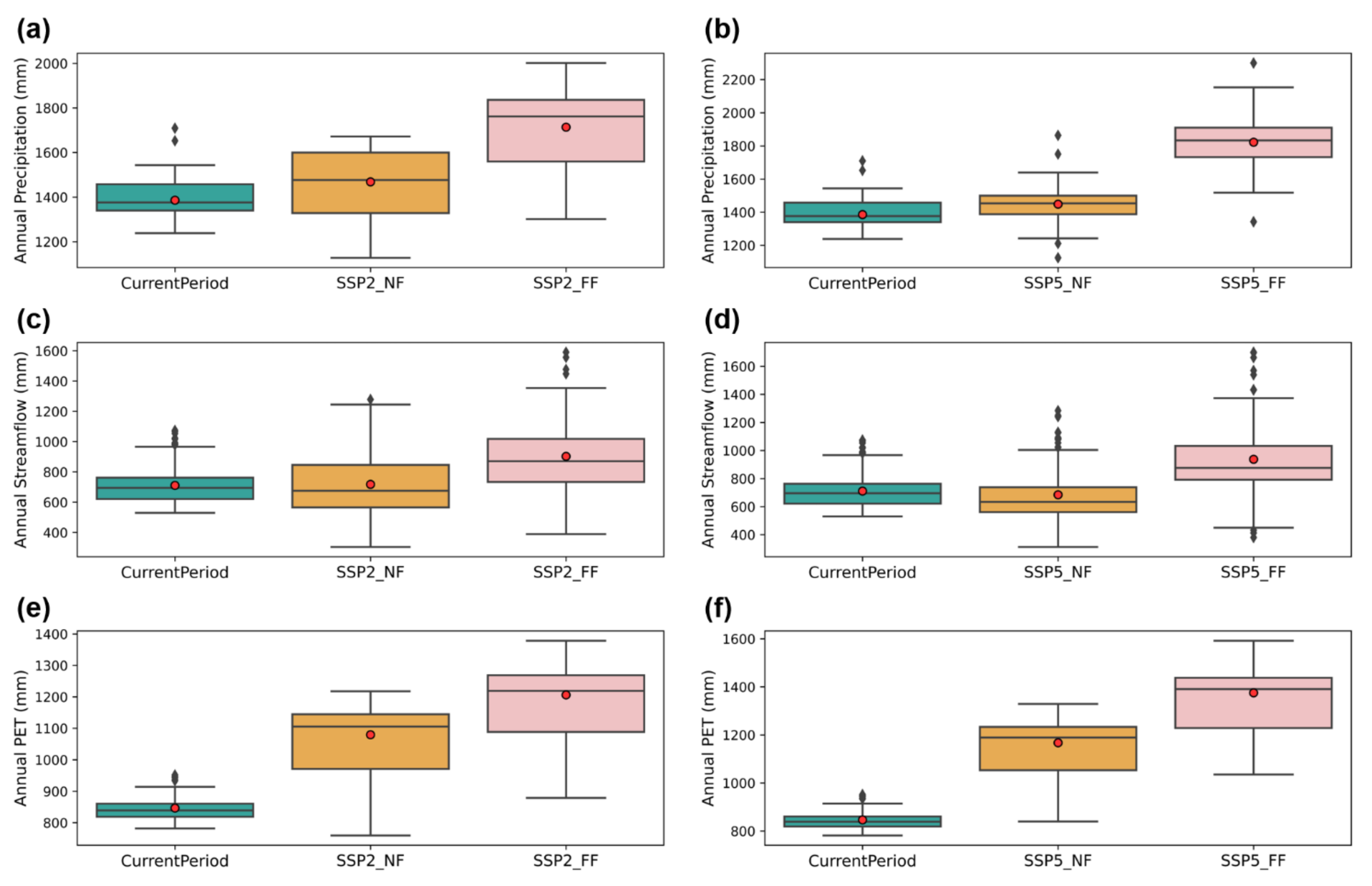
The annual changes in precipitation, streamflow, and potential evapotranspiration for 154 watersheds over time are presented in Figure 6. In the past period, an annual streamflow of approximately 461 mm on average is seen for the entire watershed. In the current period and NF under both climate change scenarios, the streamflow increased similarly by about 49–55% compared to that in the past period, and in the NF period under SSP5 scenario, the annual streamflow increased slightly less than that in the current period. The average annual streamflow during FF increased by about 96–103% compared to the past period and showed a higher increase in the SSP5 scenario.
The average annual potential evapotranspiration was 873 mm over the past period, but decreased by about 3% in the current period. Under SSP2 and SSP5 scenarios, during the NF, the increases of annual evapotranspiration were 23% and 33%, respectively, and during the FF, these were 38% and 57%, respectively.
As shown in Figure 6, the change in the amount of streamflow for each period was similar to that of the amount of precipitation, and the latter had a greater influence on the change of streamflow than the amount of potential evaporation.
3.4. Assessment of the Climate and Land Use Change Impacts on Hydrologic Conditions
We set the past period (1970–1984) as the base period, and the Budyko-type curve parameters (ω) were calculated for each of the 154 watersheds from annual rainfall, streamflow, and potential evapotranspiration. To analyze how the aridity and evaporation indices of each watershed changed from the base period under the current and climate change conditions, we visualized the direction and magnitude of the movement in the Budyko space as a wind rose diagram. As the movement in the Budyko space is the result of both climate change and land use effects, the decomposition method was used to quantify the effects of each. The amount of change in evaporation index and streamflow due to climate and land use changes, respectively, was calculated. Therefore, it was found that the hydroclimatic condition of the watershed varied depending on the direction of movement in the Budyko space, and the hydroclimatic conditions of the watershed were divided into five groups.
3.4.1. Hydroclimatic Movement in Budyko Space
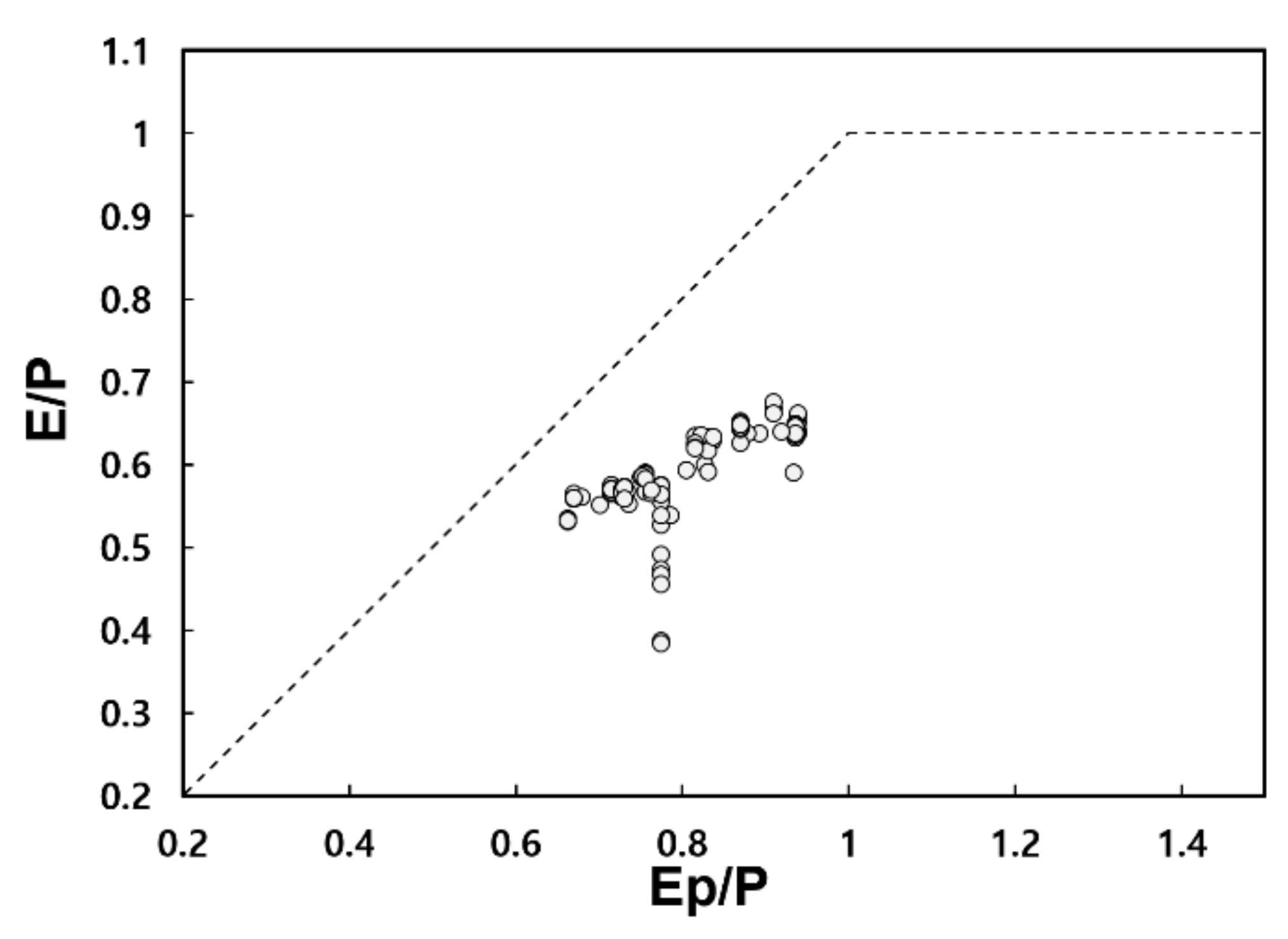
The aridity index and evaporation index values for the base year were calculated for each watershed, and the results presented in the Budyko space are shown in Figure 7. In all the watersheds, the aridity index is seen to be less than 1, which means that the HRB is in a humid state and is affected by the energy limit. To evaluate how the hydroclimatic condition changes from the past period to the present and the future, the direction and magnitude of the movement in the Budyko space were calculated, and these are shown as the roses of movements in Figure 8.
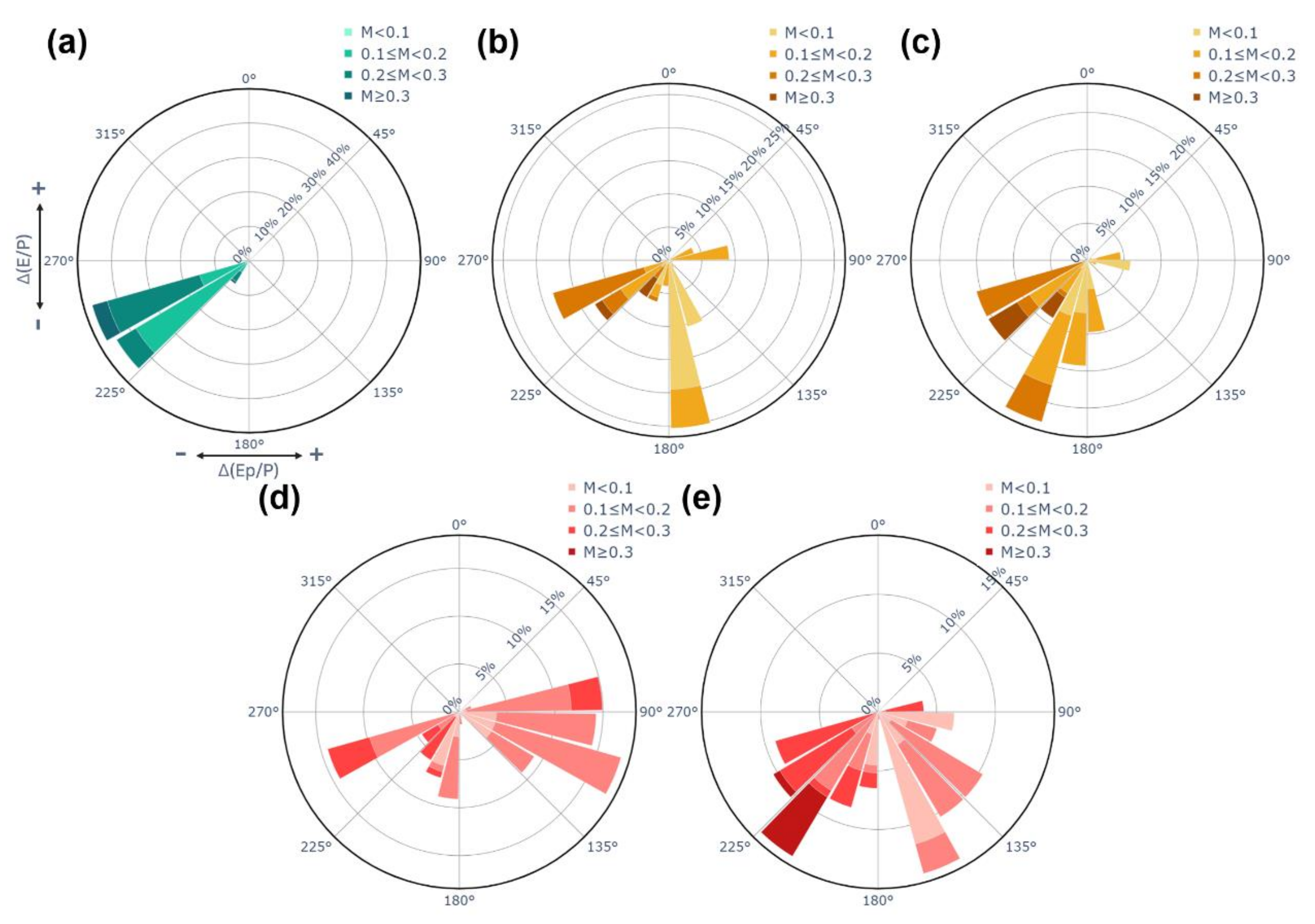
If only the effect of climate change is present, the Budyko parameter, ω, remains constant, and the direction of movements only has values in the range of 45–90° and 225–270° [35]. Thus, the direction of the other range is the result of the land use change impact. In all of the scenarios shown in Figure 8, watersheds with a direction of 90–225° appeared, which means that land use change generally caused a decrease in the evaporation index. In the current period, most of the watersheds moved to the lower left and closer to the energy limit line. It means that as the aridity index and evaporation index decreased compared to those in the past period, and the watershed became less arid and wetter. In NF, under both the SSP2 and SSP5 scenarios, both increased and decreased aridity indices were observed, and there were slightly more watersheds with increased aridity index. In addition, several watersheds showed a direction of 90–225°, which means that the hydroclimatic condition became wetter due to land use changes. During the FF, in the SSP2 scenario, most watersheds became less arid, and in the SSP5 scenario, slightly more watersheds changed to more arid conditions. In addition, as the direction of most watersheds was between 90° and 225°, it can be suggested that the decrease of evaporation index due to land use change was greater than in NF.
In this paper, due to the combined impact of land use change and climate change, most watersheds were predicted to become wetter in future scenarios. However, a different result was reported by Van der Velde et al. [33], who distinguished Sweden into three regions related to hydroclimatic change adaptation during recent years: the mountains, the forests, and the agricultural areas. Van der Velde et al. [33] showed that forest areas reacted to climate change by remaining the evaporation index constantly and that agricultural areas had an upward direction in Budyko space due to the overuse of water in agricultural areas. In contrast, in this research, by the expansion of built-up land and loss of cultivated and forest lands, it was estimated that climatic and land use changes outpaced the ability of the forests to adapt their water and energy use strategies. In addition, a decrease in water use in agricultural areas and the increase of impervious surfaces in urban areas may have contributed to the decrease in the evaporation index.
3.4.2. Relative Contribution of Climate and Land Use Changes on Hydrological Conditions
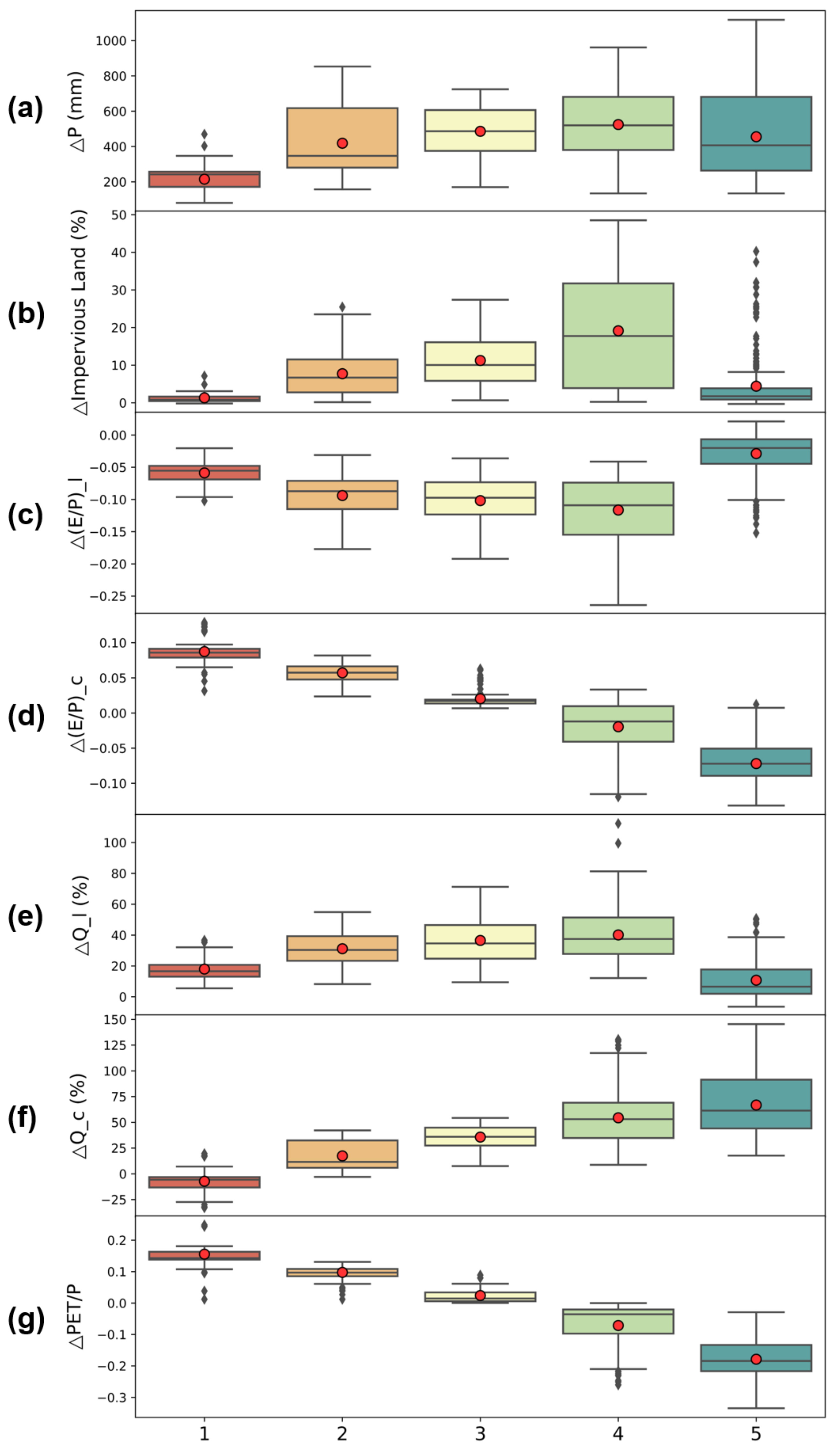
The difference in the distribution of roses of movement by period is due to the combination of climate and land use changes. Thus, the wind rose diagram only shows the general tendency of changes in the aridity and evaporation indices; limitations exist in quantitatively grasping the extent to which climate and land use changes have each affected the hydroclimatic condition changes [35]. Accordingly, we classified the hydroclimatic conditions of the watershed into five groups based on the direction of movements in Budyko space shown in Figure 8 and plotted the separation result of climate and land use impact on hydrologic conditions for each group. Table 8 presents the ranges of direction and the overall tendency of each hydrologic parameter for each hydroclimatic condition group. Figure 9 shows the box plot illustrating the amount of change in precipitation, impervious area ratio, evaporation index by climate and land use changes, streamflow by climate and land use changes, and aridity index for each group.
Groups 1 and 5 showed little changes in impervious area ratio; hence, the change in runoff due to land use change was small, and they were primarily affected by climate change. In other words, the rate of change in runoff due to climate change decreased in group 1 and increased most significantly in group 5. Furthermore, group 1 exhibited the greatest increase in the aridity index, while group 5 showed the greatest decrease. Comparing groups 2, 3, and 4, the impervious land ratio increased as we move to group 4, and accordingly, the impact of land use on the streamflow change was also greater. On the contrary, the evaporation index due to climate change decreased and increased in groups 2 and 3, respectively, but streamflow by climate change increased in groups 2, 3, and 4, and increased significantly as we move to group 4. This means that even if there is a little change in the evaporation index, streamflow can increase due to an increase in precipitation.
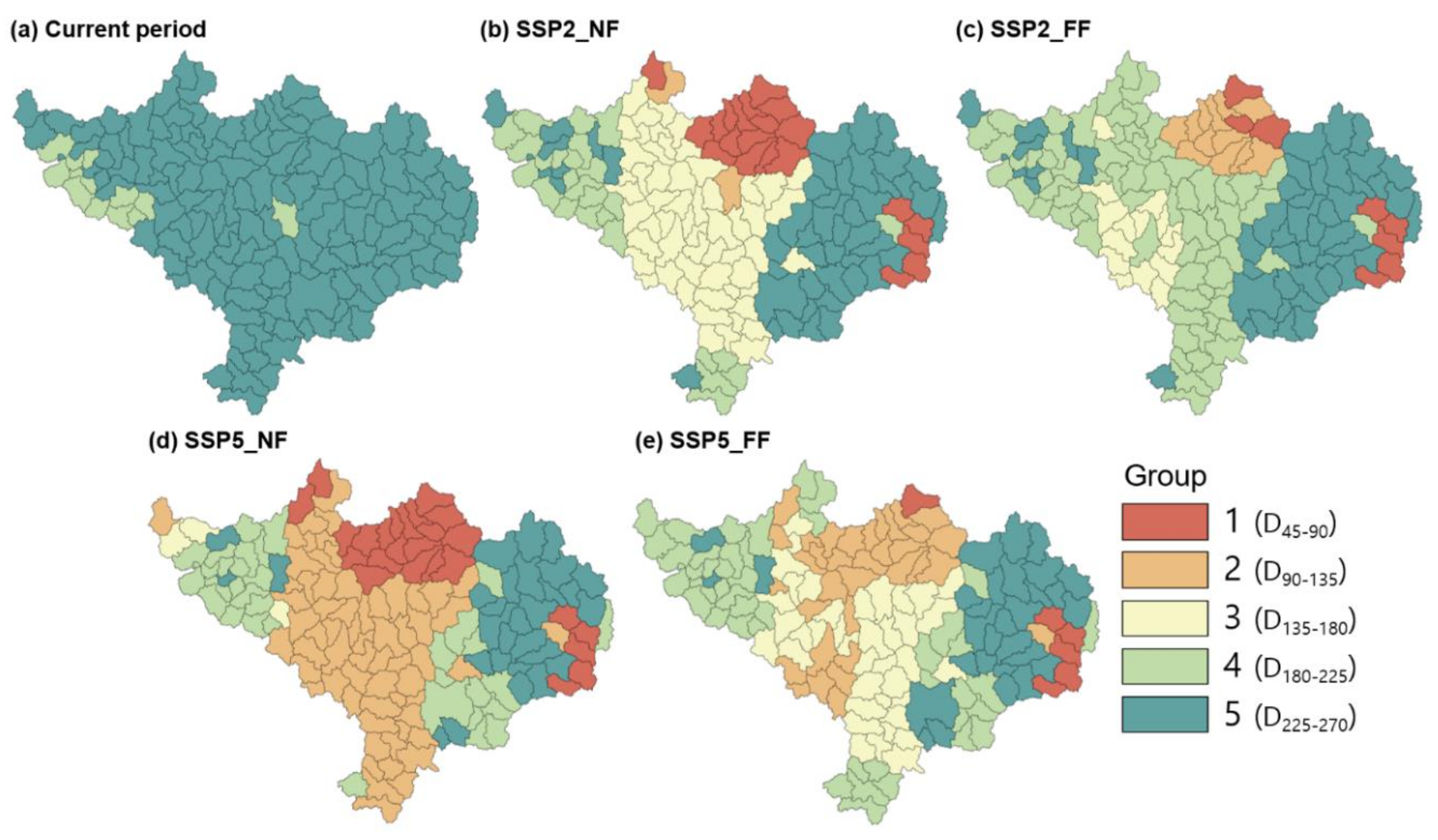
Figure 10 illustrates the distribution of hydroclimatic movement groups in HRB according to each climate and land use change conditions. In the current period, most of the regions belong to group 5; thus, it is estimated that climate change has a greater effect than land use change, and the amount of streamflow has greatly increased due to climate change. Group 4, which was highly affected by both land use and climate change, appeared in the downstream of the Seoul metropolitan area due to a significant increase of urban area in 2013, indicating that the watershed became wetter.
For NF, under both the SSP2 and SSP5 scenarios, group 4 showed a large increase in the western region of HRB, while group 1 appeared in the upper center region. Thus, it is evident that the western region is greatly affected by both land use and climate change, and while the upper central part is hardly affected by land use change, it is predicted that the streamflow will rather decrease due to climate change. The central region of HRB corresponds to groups 3 and 2 in SSP2 and SSP5, respectively, and it is expected that the increase of streamflow due to climate change in SSP2 will be greater than in SSP5.
For FF, most of the areas of group 1 during the NF period changed to group 2, and it is predicted that runoff will increase by both land use and climate change. In the central region of HRB, hydroclimatic movement group significantly changed compared to NF. Under SSP2, group 3 regions in NF were changed to group 4, and under SSP5, group 2 watersheds were changed to group 3. Thus, the effects of both climate and land use changes were found to be increased and, in particular, the impact of climate change was higher than that of the land use change. In FF, the regions corresponding to group 4 under SSP2 corresponded to groups 2 and 3 in the SSP5; hence, the probability of the watershed becoming more arid due to climate change is expected to be greater in the SSP5 scenario.
The regional distribution of each group shown in Figure 10 varies by region, but watersheds in the same neighborhood were predicted to show similar trends of movement as discussed in Heidari et al. [31]. In addition, as a result of comparing hydroclimatic movements with Heidari et al. [31], who divided climate change scenarios into DRY, MIDDLE, and WET, and analyzed hydroclimatic movement in the United States, it was analyzed that the hydroclimatic movement in the present period was similar to the distribution under the WET scenario, and the future period was similar to the distribution under the MIDDLE scenario. Meanwhile, Heidari et al. [31] and Piemontese et al. [32] also considered the effects of human activities such as regional landform, ecology, and landcover play, but the majority of river basins did not show an increase or decrease in the evaporation index and hydroclimatic movements were mainly characterized by climate change.
4. Conclusions
In this study, the hydrological model and Budyko framework were used to assess the hydroclimatic movement under future scenarios including both climate and land use changes. Comparison of hydroclimatic movement in Budyko space reveals that the aridity index decreased in all watersheds during the current period compared to the past period, while watersheds with increased aridity index were also observed in other future period scenarios. Furthermore, due to land use change, the evaporation index decreased through the appearance of watersheds with a movement direction of 90–225°. As a result of analyzing the hydrologic parameters for each hydroclimatic condition movement group, the impervious area ratio and the amount of change in runoff due to land use change (%) showed a similar pattern and was inversely proportional to the change in the evaporation index due to land use change. In addition, the amount of change in the evaporation index and dryness index due to climate change were similar and inversely proportional to the amount of runoff change (%) due to climate change. Meanwhile, the distribution of hydroclimatic movement groups for each scenario were more diversely distributed by region in future scenarios than the current period. Therefore, different adaptation strategies will be needed for each region to cope with future hydroclimatic changes.
These findings can be used as a roadmap for policymakers to prepare future water circulation improvement plans and adaptation strategies for each watershed in preparation for the upcoming climate change and increasing urban demand. It can also be used as basic data in establishing land use planning strategies, such as preparing appropriate impervious surface management measures. However, the future land cover map predicted through the model in this study does not sufficiently consider the future social and economic situation, and biophysical characteristics of each region. Therefore, if future land use prediction is performed in consideration of more diverse land use characteristics, more accurate land use change prediction will be possible in preparation for future complex environmental changes. Furthermore, this study was conducted only on a single GCM model, and if more diverse GCMs are applied to predict future hydroclimatic changes in future papers, they will be able to suggest more reliable prediction results and futuristic ideas.
Author Contributions
S.K. constructed the climate and land use data, developed hydrological model components, and prepared the manuscript; K.K. calculated the hydrological parameters; H.K. supervised the research and revised the manuscript along with S.-M.J., S.H., and M.-S.K. All authors have read and agreed to the published version of the manuscript.
Funding
This research was funded by the Korean Ministry of Environment (MOE) as “Public Technology Program based on Environmental Policy” with the grant number 2016000200001.
Institutional Review Board Statement
Not applicable.
Informed Consent Statement
Not applicable.
Data Availability Statement
The data presented in this study are available on request from the corresponding author. Some data may not be provided due to privacy.
Conflicts of Interest
The authors declare no conflict of interest.
References
- DESA, U.N. World Population Prospects 2019: Highlights; United Nations Department for Economic and Social Affairs: New York, NY, USA, 2019. [Google Scholar]
- Ouyang, T.; Zhu, Z.; Kuang, Y. Assessing Impact of Urbanization on River Water Quality In The Pearl River Delta Economic Zone, China. Environ. Monit. Assess. 2006, 120, 313–325. [Google Scholar] [CrossRef] [PubMed]
- Chithra, S.V.; Nair, M.V.H.; Amarnath, A.; Anjana, N.S. Impacts of impervious surfaces on the environment. Int. J. Eng. Sci. Invent. 2015, 4, 27–31. [Google Scholar]
- Lepeška, T. The impact of impervious surfaces on ecohydrology and health in urban ecosystems of Banská Bystrica (Slovakia). Soil Water Res. 2016, 11, 29–36. [Google Scholar] [CrossRef] [Green Version]
- Hoegh-Guldberg, O.; Jacob, D.; Taylor, M.; Bindi, M.; Brown, S.; Camilloni, I.; Diedhiou, A.; Djalante, R.; Ebi, K.; Engelbrecht, F.; et al. Impacts of 1.5 °C Global Warming on Natural and Human Systems. Available online: https://www.ipcc.ch/site/assets/uploads/sites/2/2018/12/SR15_Chapter3_Low_Res.pdf (accessed on 17 February 2021).
- Shukla, P.R.; Skea, J.; Calvo Buendia, E.; Masson-Delmotte, V.; Pörtner, H.-O.; Roberts, D.C.; Zhai, P.; Slade, R.; Connors, S.; van Diemen, R.; et al. Climate Change and Land: An IPCC Special Report on Climate Change, Desertification, Land Degradation, Sustainable Land Management, Food Security, and Greenhouse Gas Fluxes in Terrestrial Ecosystems; IPCC: Geneva, Switzerland, 2019. [Google Scholar]
- Gedney, N.; Cox, P.M.; A Betts, R.; Boucher, O.K.; Huntingford, C.; A Stott, P. Detection of a direct carbon dioxide effect in continental river runoff records. Nat. Cell Biol. 2006, 439, 835–838. [Google Scholar] [CrossRef] [PubMed]
- Jha, M.; Arnold, J.G.; Gassman, P.W.; Giorgi, F.; Gu, R.R. Climate change sensitivity assessment on upper Mississippi River basin streamflows using SWAT. J. Am. Water Resour. Ass. 2007, 42, 997–1015. [Google Scholar] [CrossRef]
- Piao, S.; Fang, J.; Ciais, P.; Peylin, P.; Huang, Y.; Sitch, S.; Wang, T. The carbon balance of terrestrial ecosystems in China. Nat. Cell Biol. 2009, 458, 1009–1013. [Google Scholar] [CrossRef]
- Ficklin, D.L.; Luo, Y.; Luedeling, E.; Zhang, M. Climate change sensitivity assessment of a highly agricultural watershed using SWAT. J. Hydrol. 2009, 374, 16–29. [Google Scholar] [CrossRef]
- Zhou, G.Y.; Wei, X.H.; Wu, Y.P.; Liu, S.G.; Huang, Y.H.; Yan, J.H.; Zhang, D.Q.; Zhang, Q.M.; Liu, J.X.; Meng, Z. Quantifying the hydrological responses to climate change using an intact forested small watershed in southern China. Glob. Chang. Biol. 2011, 17, 3736–3746. [Google Scholar] [CrossRef]
- Wu, Y.; Liu, S.; Gallant, A.L. Predicting impacts of increased CO2 and climate change on the water cycle and water quality in the semiarid James River Basin of the Midwestern USA. Sci. Total. Environ. 2012, 430, 150–160. [Google Scholar] [CrossRef] [Green Version]
- Jackson, R.B.; Carpenter, S.R.; Dahm, C.N.; Mcknight, D.M.; Naiman, R.J.; Postel, S.L.; Running, S.W. Water in a Changing World. Ecol. Appl. 2001, 11, 1027–1045. [Google Scholar] [CrossRef]
- Lu, S.; Zhang, X.; Bao, H.; Skitmore, M. Review of social water cycle research in a changing environment. Renew. Sustain. Energy Rev. 2016, 63, 132–140. [Google Scholar] [CrossRef] [Green Version]
- Miller, J.D.; Kim, H.; Kjeldsen, T.R.; Packman, J.; Grebby, S.; Dearden, R. Assessing the impact of urbanization on storm runoff in a peri-urban catchment using historical change in impervious cover. J. Hydrol. 2014, 515, 59–70. [Google Scholar] [CrossRef] [Green Version]
- Leopold, L. Hydrology for Urban Land Planning: A Guidebook on the Hydrological Effects of Urban Land Use; United State Geological Survey: Washington, DC, USA, 1986.
- Ha, K.-J.; Yun, K.-S. Climate change effects on tropical night days in Seoul, Korea. Theor. Appl. Clim. 2012, 109, 191–203. [Google Scholar] [CrossRef]
- Ahiablame, L.M.; Engel, B.A.; Chaubey, I. Effectiveness of Low Impact Development Practices: Literature Review and Suggestions for Future Research. Water, Air, Soil Pollut. 2012, 223, 4253–4273. [Google Scholar] [CrossRef]
- Elliott, A.; Trowsdale, S. A review of models for low impact urban stormwater drainage. Environ. Model. Softw. 2007, 22, 394–405. [Google Scholar] [CrossRef]
- Baek, S.-S.; Choi, D.-H.; Jung, J.-W.; Lee, H.-J.; Lee, H.; Yoon, K.-S.; Cho, K.H. Optimizing low impact development (LID) for stormwater runoff treatment in urban area, Korea: Experimental and modeling approach. Water Res. 2015, 86, 122–131. [Google Scholar] [CrossRef]
- Wilby, R.L. Evaluating climate model outputs for hydrological applications. Hydrol. Sci. J. 2010, 55, 1090–1093. [Google Scholar] [CrossRef]
- Randall, D.A.; Wood, R.A.; Bony, S.; Colman, R.; Fichefet, T.; Fyfe, J.; Kattsov, V.; Pitman, A.; Shukla, J.; Srinivasan, J.; et al. Climate models and their evaluation. In Climate Change 2007: The Physical Science Basis; Solomon, S., Qin, D., Manning, M., Chen, Z., Marquis, M., Averyt, K.B., Tignor, M., Miller, H.L., Eds.; Cambridge University Press: Cambridge, New York, NY, USA, 2007. [Google Scholar]
- Göncü, S.; Albek, E. Modeling climate change effects on streams and reservoirs with HSPF. Water Resour. Manag. 2010, 24, 707–726. [Google Scholar] [CrossRef]
- Pandey, V.P.; Dhaubanjar, S.; Bharati, L.; Thapa, B.R. Hydrological response of Chamelia watershed in Mahakali Basin to climate change. Sci. Total. Environ. 2019, 650, 365–383. [Google Scholar] [CrossRef] [PubMed]
- Chung, E.-S.; Park, K.; Lee, K.S. The relative impacts of climate change and urbanization on the hydrological response of a Korean urban watershed. Hydrol. Process. 2010, 25, 544–560. [Google Scholar] [CrossRef]
- Mango, L.M.; Melesse, A.M.; McClain, M.E.; Gann, D.; Setegn, S.G. Land use and climate change impacts on the hydrology of the upper Mara River Basin, Kenya: results of a modeling study to support better resource management. Hydrol. Earth Syst. Sci. 2011, 15, 2245–2258. [Google Scholar] [CrossRef] [Green Version]
- Xu, X.; Yang, D.; Yang, H.; Lei, H. Attribution analysis based on the Budyko hypothesis for detecting the dominant cause of runoff decline in Haihe basin. J. Hydrol. 2014, 510, 530–540. [Google Scholar] [CrossRef]
- Bhatta, B.; Shrestha, S.; Shrestha, P.K.; Talchabhadel, R. Evaluation and application of a SWAT model to assess the climate change impact on the hydrology of the Himalayan River Basin. Catena 2019, 181, 104082. [Google Scholar] [CrossRef]
- Xu, X.; Yang, H.; Yang, D.; Ma, H. Assessing the impacts of climate variability and human activities on annual runoff in the Luan River basin, China. Hydrol. Res. 2013, 44, 940–952. [Google Scholar] [CrossRef] [Green Version]
- Budyko, M.I. Evaporation under Natural Conditions; Gidrometeoizdat: Leningrad, Russia, 1963. [Google Scholar]
- Heidari, H.; Arabi, M.; Warziniack, T.; Kao, S. Assessing Shifts in Regional Hydroclimatic Conditions of U.S. River Basins in Response to Climate Change over the 21st Century. Earth’s Futur. 2020, 8, 1–14. [Google Scholar] [CrossRef]
- Piemontese, L.; Fetzer, I.; Rockström, J.; Jaramillo, F. Future Hydroclimatic Impacts on Africa: Beyond the Paris Agreement. Earths Future 2019, 7, 748–761. [Google Scholar] [CrossRef] [Green Version]
- Van Der Velde, Y.; Vercauteren, N.; Jaramillo, F.; Dekker, S.C.; Destouni, G.; Lyon, S.W. Exploring hydroclimatic change disparity via the Budyko framework. Hydrol. Process. 2013, 28, 4110–4118. [Google Scholar] [CrossRef]
- Jaramillo, F.; Destouni, G. Developing water change spectra and distinguishing change drivers worldwide. Geophys. Res. Lett. 2014, 41, 8377–8386. [Google Scholar] [CrossRef]
- Jaramillo, F.; Cory, N.; Arheimer, B.; Laudon, H.; Van Der Velde, Y.; Hasper, T.B.; Teutschbein, C.; Uddling, J. Dominant effect of increasing forest biomass on evapotranspiration: interpretations of movement in Budyko space. Hydrol. Earth Syst. Sci. 2018, 22, 567–580. [Google Scholar] [CrossRef] [Green Version]
- Zaninelli, P.G.; Menéndez, C.G.; Falco, M.; López-Franca, N.; Carril, A.F. Future hydroclimatological changes in South America based on an ensemble of regional climate models. Clim. Dyn. 2018, 52, 819–830. [Google Scholar] [CrossRef]
- Wang, D.; Hejazi, M. Quantifying the relative contribution of the climate and direct human impacts on mean annual streamflow in the contiguous United States. Water Resour. Res. 2011, 47. [Google Scholar] [CrossRef] [Green Version]
- Teng, J.; Chiew, F.H.S.; Vaze, J.; Marvanek, S.; Kirono, D.G.C. Estimation of Climate Change Impact on Mean Annual Runoff across Continental Australia Using Budyko and Fu Equations and Hydrological Models. J. Hydrometeorol. 2012, 13, 1094–1106. [Google Scholar] [CrossRef]
- Jiang, C.; Xiong, L.; Wang, D.; Liu, P.; Guo, S.; Xu, C.-Y. Separating the impacts of climate change and human activities on runoff using the Budyko-type equations with time-varying parameters. J. Hydrol. 2015, 522, 326–338. [Google Scholar] [CrossRef]
- Kazemi, H.; Sarukkalige, R.; Badrzadeh, H. Evaluation of streamflow changes due to climate variation and human activities using the Budyko approach. Environ. Earth Sci. 2019, 78, 713. [Google Scholar] [CrossRef]
- Vu, T.T.; Li, L.; Jun, K.S. Evaluation of Multi-Satellite Precipitation Products for Streamflow Simulations: A Case Study for the Han River Basin in the Korean Peninsula, East Asia. Water 2018, 10, 642. [Google Scholar] [CrossRef] [Green Version]
- Chang, H. Spatial analysis of water quality trends in the Han River basin, South Korea. Water Res. 2008, 42, 3285–3304. [Google Scholar] [CrossRef]
- Kim, H.; Jeong, H.; Jeon, J.; Bae, S. The Impact of Impervious Surface on Water Quality and Its Threshold in Korea. Water 2016, 8, 111. [Google Scholar] [CrossRef] [Green Version]
- Li, X.; Chen, G.; Liu, X.; Liang, X.; Wang, S.; Chen, Y.; Pei, F.; Xu, X. A New Global Land-Use and Land-Cover Change Product at a 1-km Resolution for 2010 to 2100 Based on Human–Environment Interactions. Ann. Am. Assoc. Geogr. 2017, 107, 1040–1059. [Google Scholar] [CrossRef]
- Liu, X.; Liang, X.; Li, X.; Xu, X.; Ou, J.; Chen, Y.; Li, S.; Wang, S.; Pei, F. A future land use simulation model (FLUS) for simulating multiple land use scenarios by coupling human and natural effects. Landsc. Urban Plan. 2017, 168, 94–116. [Google Scholar] [CrossRef]
- Liang, X.; Liu, X.; Li, D.; Zhao, H.; Chen, G. Urban growth simulation by incorporating planning policies into a CA-based future land-use simulation model. Int. J. Geogr. Inf. Sci. 2018, 32, 2294–2316. [Google Scholar] [CrossRef]
- Chen, Y.; Li, X.; Liu, X.; Ai, B. Modeling urban land-use dynamics in a fast developing city using the modified logistic cellular automaton with a patch-based simulation strategy. Int. J. Geogr. Inf. Sci. 2014, 28, 234–255. [Google Scholar] [CrossRef]
- Hamad, R.; Balzter, H.; Kolo, K. Predicting Land Use/Land Cover Changes Using a CA-Markov Model under Two Different Scenarios. Sustainability 2018, 10, 3421. [Google Scholar] [CrossRef] [Green Version]
- Arsanjani, J.J.; Kainz, W.; Mousivand, A.J. Tracking dynamic land-use change using spatially explicit Markov Chain based on cellular automata: the case of Tehran. Int. J. Image Data Fusion 2011, 2, 329–345. [Google Scholar] [CrossRef]
- Yang, X.; Zheng, X.-Q.; Chen, R. A land use change model: Integrating landscape pattern indexes and Markov-CA. Ecol. Model. 2014, 283, 1–7. [Google Scholar] [CrossRef]
- Donigian, A.S., Jr.; Bicknell, B.R.; Imhoff, J.C. Hydrological Simulation Program—FORTRAN (HSPF). In Computer Models of Watershed Hydrology; Singh, V.P., Ed.; Water Resources Pubs: Highlands Ranch, CO, USA, 1995; pp. 395–442. [Google Scholar]
- Stern, M.; Flint, L.; Minear, J.; Flint, A.; Wright, S. Characterizing Changes in Streamflow and Sediment Supply in the Sacramento River Basin, California, Using Hydrological Simulation Program—FORTRAN (HSPF). Water 2016, 8, 432. [Google Scholar] [CrossRef] [Green Version]
- Albek, M.; Bakır Öğütveren, Ü.; Albek, E. Hydrological Modeling of Seydi Suyu Watershed (Turkey) with HSPF. J. Hydrol. 2004, 285, 260–271. [Google Scholar] [CrossRef]
- Diaz-Ramirez, J.N.; Perez-Alegria, L.R.; McAnally, W.H. Hydrology and Sediment Modeling Using BASINS/HSPF in a Tropical Island Watershed. Trans. ASABE 2008, 51, 1555–1565. [Google Scholar] [CrossRef]
- Moriasi, D.N.; Gitau, M.W.; Pai, N.; Daggupati, P. Hydrologic and Water Quality Models: Performance Measures and Evaluation criteria. Trans. ASABE 2015, 58, 1763–1785. [Google Scholar]
- Berghuijs, W.; Greve, P. A review of the Budyko water balance framework. In Proceedings of the EGU General Assembly, Vienna, Austria, 12–17 April 2015; pp. 12–17. [Google Scholar]
- Budyko, M.I. Climate and Life; Academic Press: Cambridge, MA, USA, 1974. [Google Scholar]
- Zhang, L.; Dawes, W.R.; Walker, G.R. Response of mean annual evapotranspiration to vegetation changes at catchment scale. Water Resour. Res. 2001, 37, 701–708. [Google Scholar] [CrossRef]
- Patterson, L.A.; Lutz, B.D.; Doyle, M.W. Climate and direct human contributions to changes in mean annual streamflow in the South Atlantic, USA. Water Resour. Res. 2013, 49, 7278–7291. [Google Scholar] [CrossRef]
- Ma, Z.; Kang, S.; Zhang, L.; Tong, L.; Su, X. Analysis of impacts of climate variability and human activity on streamflow for a river basin in arid region of northwest China. J. Hydrol. 2008, 352, 239–249. [Google Scholar] [CrossRef]
- Turc, L. Calcul du Bilan de l’Eau: Evaluation en Function des Precipitation et des Temperatures. IAHS Publ. 1954, 37, 88–200. [Google Scholar]
- Pike, J. The estimation of annual run-off from meteorological data in a tropical climate. J. Hydrol. 1964, 2, 116–123. [Google Scholar] [CrossRef]
- Fu, B. On the calculation of the evaporation from land surface. J. Atmos. Sci. 1981, 5, 23–31. [Google Scholar]
- Zhang, L.; Hickel, K.; Dawes, W.R.; Chiew, F.H.S.; Western, A.W.; Briggs, P.R. A rational function approach for estimating mean annual evapotranspiration. Water Resour. Res. 2004, 40, 40. [Google Scholar] [CrossRef]
- Porporato, A.; Daly, E.; Rodriguez-Iturbe, I. Soil Water Balance and Ecosystem Response to Climate Change. Am. Nat. 2004, 164, 625–632. [Google Scholar] [CrossRef] [PubMed]
- Wang, D.; Tang, Y. A one-parameter Budyko model for water balance captures emergent behavior in darwinian hydrologic models. Geophys. Res. Lett. 2014, 41, 4569–4577. [Google Scholar] [CrossRef] [Green Version]
- Greve, P.; Orlowsky, B.; Mueller, B.; Sheffield, J.; Reichstein, M.; Seneviratne, S.I. Global assessment of trends in wetting and drying over land. Nat. Geosci. 2014, 7, 716–721. [Google Scholar] [CrossRef]
- Gudmundsson, L.; Greve, P.; Seneviratne, S.I. The sensitivity of water availability to changes in the aridity index and other factors-A probabilistic analysis in the Budyko space. Geophys. Res. Lett. 2016, 43, 6985–6994. [Google Scholar] [CrossRef] [Green Version]
- Pontius, R.G.; Boersma, W.; Castella, J.-C.; Clarke, K.; De Nijs, T.; Dietzel, C.; Duan, Z.; Fotsing, E.; Goldstein, N.; Kok, K.; et al. Comparing the input, output, and validation maps for several models of land change. Ann. Reg. Sci. 2008, 42, 11–37. [Google Scholar] [CrossRef] [Green Version]
- Chen, Y.; Liu, X.; Li, X. Calibrating a Land Parcel Cellular Automaton (LP-CA) for urban growth simulation based on ensemble learning. Int. J. Geogr. Inf. Sci. 2017, 31, 2480–2504. [Google Scholar] [CrossRef]
- Li, Z.; Cheng, X.; Han, H. Future Impacts of Land Use Change on Ecosystem Services under Different Scenarios in the Ecological Conservation Area, Beijing, China. Forests 2020, 11, 584. [Google Scholar] [CrossRef]
- Kriegler, E.; Edmonds, J.; Hallegatte, S.; Ebi, K.L.; Kram, T.; Riahi, K.; Winkler, H.; Van Vuuren, D.P. A new scenario framework for climate change research: the concept of shared climate policy assumptions. Clim. Chang. 2014, 122, 401–414. [Google Scholar] [CrossRef] [Green Version]
Figure 1.
Han River Basin.

Figure 2.
Comparison of observed and simulated streamflow of station code (a) 1004A70 and (b) 1007A57 for the calibration and validation periods.
Figure 2.
Comparison of observed and simulated streamflow of station code (a) 1004A70 and (b) 1007A57 for the calibration and validation periods.

Figure 3.
Variation on Budyko curve according to climate change and human activities (The watershed state in the prechange period, A; the shifted state induced by climate change, B*; the shifted state induced by both climate change and human interferences, B; evaporation index in state A, (E/P)0; evaporation index in state B*, (E/P)1*; evaporation index in state B, (E/P)1; aridity index in state A, (Ep/P)0; aridity index in state B* and B, (Ep/P)1).

Figure 4.
(a) Actual and (b) simulated land use map in 2013.

Figure 5.
Actual land use map in 1975 and 2013 and predicted land use map in 2051 and 2089.

Figure 6.
Boxplot of annual precipitation, streamflow, and potential evapotranspiration (PET) for the current period, NF, and FF for two climate change scenarios: (a) annual precipitation under SSP2 scenario; (b) annual precipitation under SSP5 scenario; (c) annual streamflow under SSP2 scenario; (d) annual streamflow under SSP5 scenario; (e) annual potential evapotranspiration under SSP2 scenario; (f) annual potential evapotranspiration under SSP5 scenario

Figure 7.
Distribution of hydroclimatic condition in Budyko space of 154 watersheds in the past period (1970–1984) in terms of the aridity index (Ep/P) and evaporation index (E/P).
Figure 7.
Distribution of hydroclimatic condition in Budyko space of 154 watersheds in the past period (1970–1984) in terms of the aridity index (Ep/P) and evaporation index (E/P).

Figure 8.
Roses of movement in Budyko space for the 154 watersheds due to changes in aridity index (Ep/P) and evaporation index (E/P) between past and current and future periods: (a) current period; (b) SSP2_NF; (c) SSP2_FF; (d) SSP5_NF; (e) SSP5_FF.
Figure 8.
Roses of movement in Budyko space for the 154 watersheds due to changes in aridity index (Ep/P) and evaporation index (E/P) between past and current and future periods: (a) current period; (b) SSP2_NF; (c) SSP2_FF; (d) SSP5_NF; (e) SSP5_FF.

Figure 9.
Boxplots showing the patterns of change in (a) precipitation, (b) impervious land (%), (c) evaporation index by land use change, (d) evaporation index by climate change, (e) runoff by land use change (%), (f) runoff by climate change (%), (g) aridity index for each group.
Figure 9.
Boxplots showing the patterns of change in (a) precipitation, (b) impervious land (%), (c) evaporation index by land use change, (d) evaporation index by climate change, (e) runoff by land use change (%), (f) runoff by climate change (%), (g) aridity index for each group.

Figure 10.
Map of Han River Basin (HRB) clustered according to the five hydroclimatic movement regions for (a) current period (b) SSP2_NF, (c) SSP2_FF, (d) SSP5_NF, and (e) SSP5_FF.
Figure 10.
Map of Han River Basin (HRB) clustered according to the five hydroclimatic movement regions for (a) current period (b) SSP2_NF, (c) SSP2_FF, (d) SSP5_NF, and (e) SSP5_FF.


Table 1.
List of data used in future land use simulation (FLUS) and data sources. DEM, digital elevation model.
Table 1.
List of data used in future land use simulation (FLUS) and data sources. DEM, digital elevation model.
| Data | Data Description | Data Sources |
|---|---|---|
| Land Use 1975 | Land Use in 1975 at 30 m Spatial Resolution | Water Resources Management Information System (WAMIS). Available online: http://www.wamis.go.kr/ (accessed on 11 March 2021) |
| Land Use 2013 | Land use in 2013 at 30 m Spatial resolution | Environmental Geographic Information Service. Available online: https://egis.me.go.kr/ (accessed on 11 March 2021) |
| DEM | Digital Elevation Model with 30 m Spatial Resolution | National Geographic Information Institute (NGII). Available online: http://map.ngii.go.kr/ (accessed on 11 March 2021) |
| Aspect | Direction of the Maximum Rate of Change in the z–Value from Each Cell | Calculated from DEM data |
| Slope | Rate of Maximum Change in z-Value from Each Cell | Calculated from DEM data |
| Distance from Rivers | Distance from Rivers Calculated by Euclidean Distance Tool in ArcGIS | Water resources Management Information System (WAMIS). Available online: http://www.wamis.go.kr/ (accessed on 11 March 2021) |
Table 2.
Total land demand pixels.
| Year | Built-up Land | Agricultural Land | Forest Land | Grassland | Wetland | Barren Land | Water |
|---|---|---|---|---|---|---|---|
| 1975 | 314799 | 4249147 | 14877935 | 303125 | 60170 | 180553 | 259414 |
| 2013 | 1408033 | 3173318 | 13872451 | 762706 | 141250 | 386489 | 500897 |
| 2051 | 2085907 | 2917205 | 13121831 | 801746 | 149797 | 423515 | 745142 |
| 2089 | 2511200 | 2834317 | 12530224 | 810935 | 157494 | 444566 | 956406 |
Remarks: Size of each pixel is 30 × 30, that is, area of a pixel is 900 m2.
Table 3.
Calibrated values of Hydrological Simulation Program-Fortran (HSPF) parameters.
| Parameter | Definition | Units | Original Value | Calibrated Value |
|---|---|---|---|---|
| FOREST | Pervious Land Fraction Covered by Forest | none | 0–1 | 0–1 |
| INFILT | Index to Infiltration Capacity | In/h | 0.16 | 0.01–0.03 |
| LSUR | Length of Overland Flow | feet | 150–250 | 150–350 |
| SLSUR | Slope of Overland Flow Plane | none | - | 0.001–0.885 |
| INTFW | Interflow Inflow Parameter | none | 0.75 | 3 |
Table 4.
Minimum, maximum, and average values of the coefficient of determination (R2), Nash-Sutcliffe coefficient of efficiency (NSE), and percent bias (PBIAS) in daily streamflow calibration and validation for 30 unit watersheds.
Table 4.
Minimum, maximum, and average values of the coefficient of determination (R2), Nash-Sutcliffe coefficient of efficiency (NSE), and percent bias (PBIAS) in daily streamflow calibration and validation for 30 unit watersheds.
| Calibration | Validation | |||||
|---|---|---|---|---|---|---|
| R2 | NSE | PBIAS | R2 | NSE | PBIAS | |
| Minimum | 0.79 | 0.37 | 0.01 | 0.70 | 0.12 | 0.01 |
| Maximum | 0.99 | 0.99 | 37.94 | 0.99 | 0.99 | 58.10 |
| Average | 0.91 | 0.73 | 14.10 | 0.88 | 0.69 | 18.43 |
Table 5.
Confusion matrix of the predicted land use versus the actual land use in 2013.
| Land Use Types | Actual Land Use in 2013 | |||||||
|---|---|---|---|---|---|---|---|---|
| Built-up Land | Cultivated Land | Forest Land | Grassland | Wetland | Barren Land | Water | Total | |
| Built-up Land | 5915 | 3107 | 2853 | 839 | 209 | 563 | 498 | 13984 |
| Agricultural Land | 4036 | 16238 | 7925 | 1571 | 550 | 1103 | 848 | 32266 |
| Forest Land | 2090 | 7626 | 123620 | 4063 | 209 | 1367 | 404 | 139309 |
| Grassland | 1036 | 1915 | 3500 | 739 | 60 | 251 | 94 | 7591 |
| Wetland | 213 | 256 | 235 | 102 | 74 | 54 | 442 | 1376 |
| Barren Land | 503 | 1729 | 746 | 271 | 99 | 307 | 176 | 3830 |
| Water | 174 | 880 | 84 | 74 | 175 | 140 | 2563 | 4090 |
| Total | 13967 | 31751 | 138963 | 7659 | 1376 | 3785 | 5025 | 202526 |
Kappa coefficient = 0.47 and overall accuracy = 0.74.
Table 6.
Area and percent for each land use type during the years 1975, 2013, 2051, and 2089.
| Land Use Types | 1975 (km2/%) | 2013 (km2/%) | 2051 (km2/%) | 2089 (km2/%) | Change (km2/%) | ||
|---|---|---|---|---|---|---|---|
| 1975–2013 | 2013–2051 | 2013–2089 | |||||
| Built-up Land | 283.32 | 1267.19 | 1877.32 | 2260.08 | 983.87 | 609.99 | 992.75 |
| (1.55) | (6.95) | (10.30) | (12.40) | (5.40) | (3.35) | (5.45) | |
| Cultivated Land | 3824.16 | 2855.89 | 2625.48 | 2550.89 | −968.27 | −231.09 | −305.69 |
| (20.99) | (15.67) | (14.40) | (13.99) | (−5.31) | (−1.27) | (−1.68) | |
| Forest Land | 13389.63 | 12484.79 | 11816.37 | 11714.46 | −904.84 | −674.44 | −776.35 |
| (73.49) | (68.52) | (64.83) | (64.27) | (−4.97) | (−3.70) | (−4.26) | |
| Grassland | 272.8 | 686.41 | 721.57 | 729.84 | 413.62 | 34.79 | 43.06 |
| (1.50) | (3.77) | (3.96) | (4.00) | (2.27) | (0.19) | (0.24) | |
| Wetland | 54.15 | 127.12 | 134.82 | 141.74 | 72.97 | 7.70 | 14.62 |
| (0.30) | (0.70) | (0.74) | (0.78) | (0.40) | (0.04) | (0.08) | |
| Barren Land | 162.5 | 347.83 | 381.16 | 400.11 | 185.33 | 33.22 | 52.17 |
| (0.89) | (1.91) | (2.09) | (2.2) | (1.02) | (0.18) | (0.29) | |
| Water | 233.47 | 450.79 | 670.63 | 430.23 | 217.32 | 219.83 | −20.57 |
| (1.28) | (2.47) | (3.68) | (2.36) | (1.19) | (1.21) | (−0.11) | |
Table 7.
Projected annual precipitation (mm) and annual mean temperature at the study area for the past period, current period, near future (NF), and far future (FF) under two shared socioeconomic pathways (SSPs) scenarios.
Table 7.
Projected annual precipitation (mm) and annual mean temperature at the study area for the past period, current period, near future (NF), and far future (FF) under two shared socioeconomic pathways (SSPs) scenarios.
| Annual Precipitation (mm) | ||||
|---|---|---|---|---|
| Past Period | Mean | 1116.2 | 11.3 | |
| Range | 982.14–1242.1 | 10.4–12.0 | ||
| Current Period | Mean Range | 1386.1 (+24.19%) | 11.6 (+2.05%) | |
| 1238.4–1709.3 | 10.9–12.4 | |||
| SSP2 | NF | Mean | 1468.7 (+31.59%) | 15.0 (+32.48%) |
| Range | 1127.7–1672.4 | 13.9–16.0 | ||
| FF | Mean | 1714.0 (+53.57%) | 16.9 (+49.39%) | |
| Range | 1301.3–2001.8 | 16.1–18.1 | ||
| SSP5 | NF | Mean | 1448.8 (+29.81%) | 16.5 (+45.54%) |
| Range | 1125.1–1863.5 | 15.1–18.0 | ||
| FF | Mean | 1822.3 (+63.27%) | 20.4 (+79.84%) | |
| Range | 1342.4–2300.0 | 18.4–22.2 | ||
Table 8.
Hydroclimatic condition group classified according to the direction of movement in the Budyko space (changes of evaporation index due to land use change, Δ(E/P)_l; changes of evaporation index due to climate change, Δ(E/P)_c; changes of runoff due to land use change, ΔQ_l; changes of runoff due to climate change, ΔQ_c; changes of aridity index, Δ(PET/P)).
| Group | Direction | Δ(E/P)_l | Δ(E/P)_c | ΔQ_l | ΔQ_c | Δ(PET/P) |
|---|---|---|---|---|---|---|
| 1 | 45°—90° | + | + | + | - | + |
| 2 | 90°—135° | + | + | + | + | + |
| 3 | 135°—180° | + | + | + | + | + |
| 4 | 180°—225° | + | - | + | + | - |
| 5 | 225°—270° | + | - | + | + | - |
Publisher’s Note: MDPI stays neutral with regard to jurisdictional claims in published maps and institutional affiliations. |
© 2021 by the authors. Licensee MDPI, Basel, Switzerland. This article is an open access article distributed under the terms and conditions of the Creative Commons Attribution (CC BY) license (https://creativecommons.org/licenses/by/4.0/).
Share and Cite
MDPI and ACS Style
Kim, S.; Kim, H.; Kim, K.; Jun, S.-M.; Hwang, S.; Kang, M.-S. Assessing the Hydroclimatic Movement under Future Scenarios Including both Climate and Land Use Changes. Water 2021, 13, 1120. https://doi.org/10.3390/w13081120
AMA Style
Kim S, Kim H, Kim K, Jun S-M, Hwang S, Kang M-S. Assessing the Hydroclimatic Movement under Future Scenarios Including both Climate and Land Use Changes. Water. 2021; 13(8):1120. https://doi.org/10.3390/w13081120
Chicago/Turabian StyleKim, Sinae, Hakkwan Kim, Kyeung Kim, Sang-Min Jun, Soonho Hwang, and Moon-Seong Kang. 2021. "Assessing the Hydroclimatic Movement under Future Scenarios Including both Climate and Land Use Changes" Water 13, no. 8: 1120. https://doi.org/10.3390/w13081120
Note that from the first issue of 2016, this journal uses article numbers instead of page numbers. See further details here.