
Laboratory and In Situ Determination of Hydraulic Conductivity and Their Validity in Transient Seepage Analysis


1
Department of Civil Engineering and Construction, Georgia Southern University, Statesboro, GA 30460, USA
2
Department of Civil and Environmental Engineering, Colorado School of Mines, Golden, CO 80401, USA
3
Department of Civil and Environmental Engineering, Lehigh University, Bethlehem, PA 18015, USA
4
US Army Corps of Engineers, Los Angeles District, Los Angeles, CA 90017, USA
*
Author to whom correspondence should be addressed.
Water 2021, 13(8), 1131; https://doi.org/10.3390/w13081131
Submission received: 21 March 2021
/
Revised: 9 April 2021
/
Accepted: 16 April 2021
/
Published: 20 April 2021
(This article belongs to the Section Hydrology)
Abstract
:This paper critically compares the use of laboratory tests against in situ tests combined with numerical seepage modeling to determine the hydraulic conductivity of natural soil deposits. Laboratory determination of hydraulic conductivity used the constant head permeability and oedometer tests on undisturbed Shelby tube and block soil samples. The auger hole method and Guelph permeameter tests were performed in the field. Groundwater table elevations in natural soil deposits with different hydraulic conductivity values were predicted using finite element seepage modeling and compared with field measurements to assess the various test results. Hydraulic conductivity values obtained by the auger hole method provide predictions that best match the groundwater table’s observed location at the field site. This observation indicates that hydraulic conductivity determined by the in situ test represents the actual conditions in the field better than that determined in a laboratory setting. The differences between the laboratory and in situ hydraulic conductivity values can be attributed to factors such as sample disturbance, soil anisotropy, fissures and cracks, and soil structure in addition to the conceptual and procedural differences in testing methods and effects of sample size.
1. Introduction
Understanding and predicting water movement or seepage in soils is a vital part of hydraulic and geotechnical engineering. The movement of water through soil is generally slow and assumed to be laminar. This flow is described by Darcy’s law, which states that the velocity of a flowing liquid (v) through a porous medium is directly proportional to the pressure gradient causing the flow and is the product of the hydraulic gradient (i) and the hydraulic conductivity (k). Darcy’s law is also valid in unsaturated soils, but the hydraulic conductivity becomes a function of the water content or the matric suction. Yet, hydraulic conductivity is the most critical parameter used to understand the flow of water through soils. An accurate determination of k is necessary for various applications in either steady-state or transient conditions. For example, analyzing the spatial and temporal variations in groundwater in response to stream elevation fluctuation is essential for groundwater storage and recharge [1,2]. Evaluating slopes with rain events or fluctuating water levels becomes a common approach to better understand the slopes’ stability [3,4]. From the environmental perspective, analyzing the transport and removal of contaminants or pathogenic viruses is also an interesting issue requiring hydraulic conductivity [5,6].
In general, the hydraulic conductivity can be determined using either indirect or direct methods. Indirect methods are based on empirical equations that take into account soil properties such as particle size distribution or void ratio. Most indirect methods are based on the fundamental theory of flow through porous media modeled as a system of circular cross-sectional tubes of different diameters [7]. Thus, these methods generally work better with granular soils than fine-grained soils. As a result, the application of indirect methods is usually limited to sandy soils.
In contrast, direct methods are based on laboratory tests with undisturbed or re-constituted samples and in situ tests where flow conditions are closer to field conditions. Laboratory tests are performed under controlled conditions such as constant cross-sectional area and constant hydraulic gradient or flow rate. The ability to impose a desired set of conditions constitutes the main advantage of laboratory testing. Nevertheless, using small test samples under one-dimensional flow conditions limits this approach’s ability to represent actual field conditions. Thus, in situ tests are often conducted because of the advantage of accounting for the complexity of field conditions more accurately than laboratory tests. In addition, sample disturbance is likely during removal and transportation and can be avoided using in situ tests.
The differences observed between laboratory hydraulic conductivity (kL) and in situ hydraulic conductivity (kF) are frequently unpredictable, with values often differing by several orders of magnitude. Most often, kF is larger than kL, including one case where the in situ value was up to 46,000 times larger than the laboratory value [8]. On the other hand, some researchers have reported the conductivity in the lab to be slightly larger [9,10]. However, these results cannot be generalized because flow characteristics, particularly in fine soils, can vary significantly depending on several factors. Therefore, the determination of hydraulic conductivity requires careful execution of tests and proper selection of experimental methods that consider field conditions’ variability.
When the hydraulic conductivity shows a wide range of variation, it is vital that the most representative value is selected; thus, utilizing information from other sources is recommended to increase the reliability. One example is that a simple field monitoring of the groundwater table (GWT) combined with transient seepage analysis can verify the validity of the hydraulic conductivity. Namely, the modeling results for various hydraulic conductivity values and the observed GWT at different locations and different flow events can be compared to determine a reliable input value and measuring technique of hydraulic conductivity. Solving such issues using numerical modeling has become very popular thanks to advances in computing resources.
This study aims to critically evaluate laboratory and in situ tests for hydraulic conductivity and check their validity with transient seepage analysis. The study is performed using natural soil deposits along the riverbank of the lower Roanoke River, North Carolina, USA. The numerical models consider the unsaturated soil properties and fluctuations of the water surface elevation (WSE) are created. Different hydraulic conductivity values obtained from four other laboratory and in situ tests are applied. The transient seepage analysis is conducted considering the fluctuations of the WSE, and the modeling results, which are the predicted phreatic surfaces in the riverbank, are compared to the monitored GWTs in the field. Four different testing methods are applied to determine the soil samples’ hydraulic conductivity collected from the riverbanks, and their values are compared. The reasons for the differences are reviewed and discussed. The validity of the selected value is verified by comparing the observed GWTs in the field to those from the numerical analysis.
2. Test Materials and Methods
2.1. Site Description and Materials
2.1.1. Study Sites
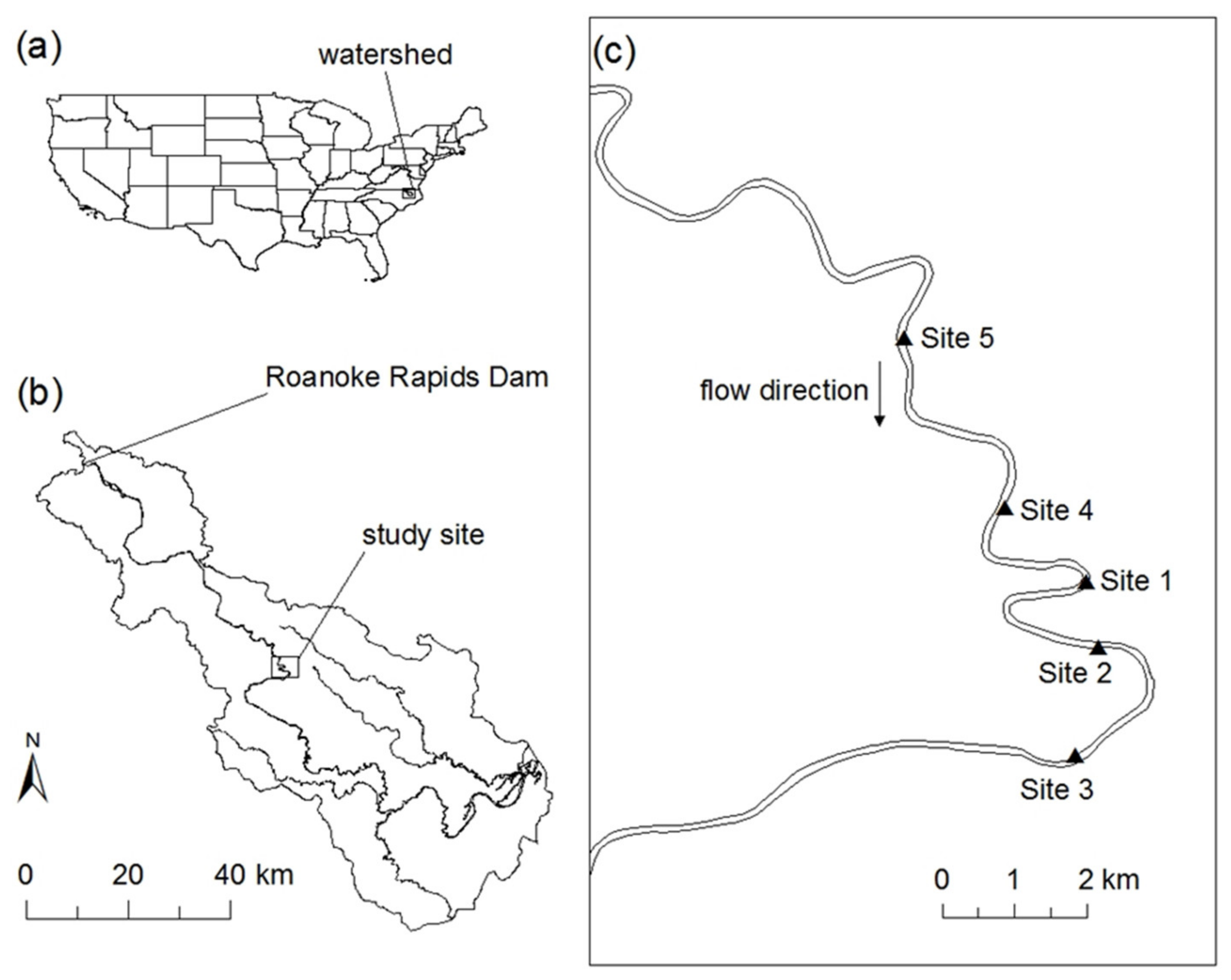
The study sites used for soil sampling, groundwater monitoring, and transient seepage analysis are located on the lower Roanoke River near Scotland Neck, North Carolina, U.S.A. (Figure 1). The lower Roanoke River flows through the northern Coastal Plain in eastern North America. The surface soil consists of Quaternary alluvium with Miocene and Upper Cretaceous sedimentary materials underlying the alluvium soil layer [11,12]. Unconsolidated fine sands, silts, and clays are the primary materials, but there are also clayey Miocene deposits in places [12,13,14]. Three significant reservoirs—Kerr Lake, Lake Gaston, and Roanoke Rapids Lake—were created after the construction of Kerr Dam, Gaston Dam, and Roanoke Rapids Dam, respectively. The Roanoke Rapids Dam is located about 72 km upstream from the sampling sites, as shown in Figure 1. Depending on the time of year and prevailing hydrologic conditions, the dam operates in one of four operational modes: normal, flood control, fish spawning, and drought flow. It is worth mentioning that 88% of the Roanoke River basin area, including all three major reservoirs, is located upstream from the Roanoke Rapids Dam [15]. No significant tributaries are present between Roanoke Rapids Dam and the study sites. Therefore, the WSE at the study sites is primarily controlled by the Roanoke Rapids Dam’s discharge. Thus, the downstream WSE can be estimated based on the dam operational mode, supplemented by observed data from the United States Geological Survey (USGS) gage stations.
As shown in Figure 1, five sites were initially selected as study sites considering the current bank retreat, accessibility, soil conditions, and peaking effect by the dam operations. After multiple site investigations, site 1 was selected for extensive laboratory and in situ studies and numerical modeling.
2.1.2. Soil Samples and Properties
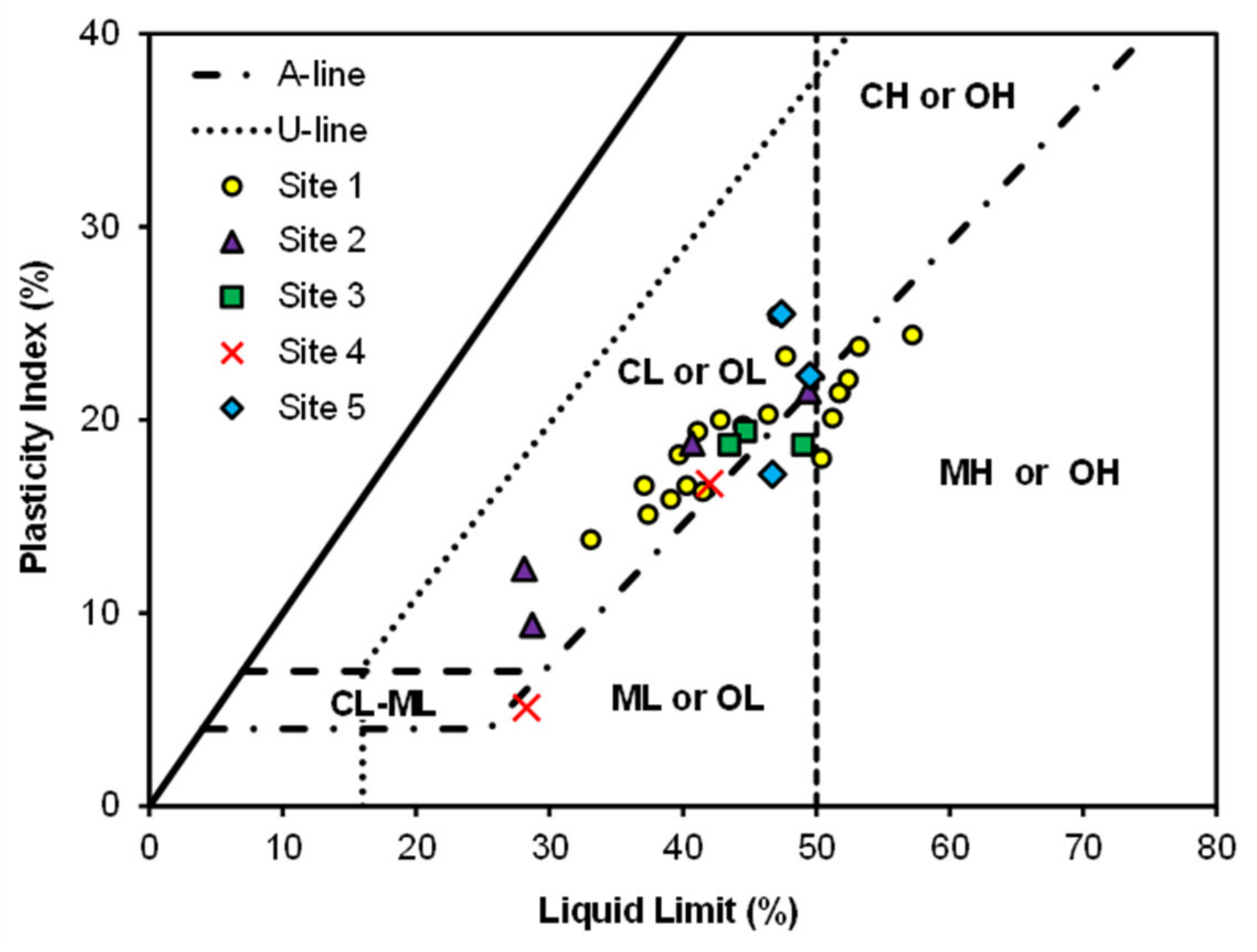
Soil samples were collected from holes drilled vertically down to 3 m from the riverbanks’ top and slope surfaces using a hand auger. These samples were analyzed for water content, void ratio, grain size distribution, specific gravity, and Atterberg limits. The riverbanks’ top surface soil layer at the study sites consists of sandy soil, classified as silty sand (SM) by the Unified Soil Classification System (USCS). The top sandy soil layer is less than 0.5 m deep, and roots and decomposed debris were observed in the samples. The soil below the top of the bank consisted of thick layers of fine-grained soils with the lower clayey layer containing lenses of gray Miocene clay. The fine-grained soils collected at multiple locations were classified as either low plasticity clay (CL), low plasticity silt (ML), or high plasticity silt (MH) by the USCS. However, no distinctive continuous horizontal seams were visible at the field sites. Despite the different classifications in the USCS, the soils were relatively similar in terms of engineering properties. The physical properties of the other soil groups are shown in Table 1 and Figure 2. The lower fine-grained soil layer’s depth was measured to be up to 6 m from the bank top. The numerical model assumed that this soil layer extends down to 10 m and is underlain by an impervious soil layer.
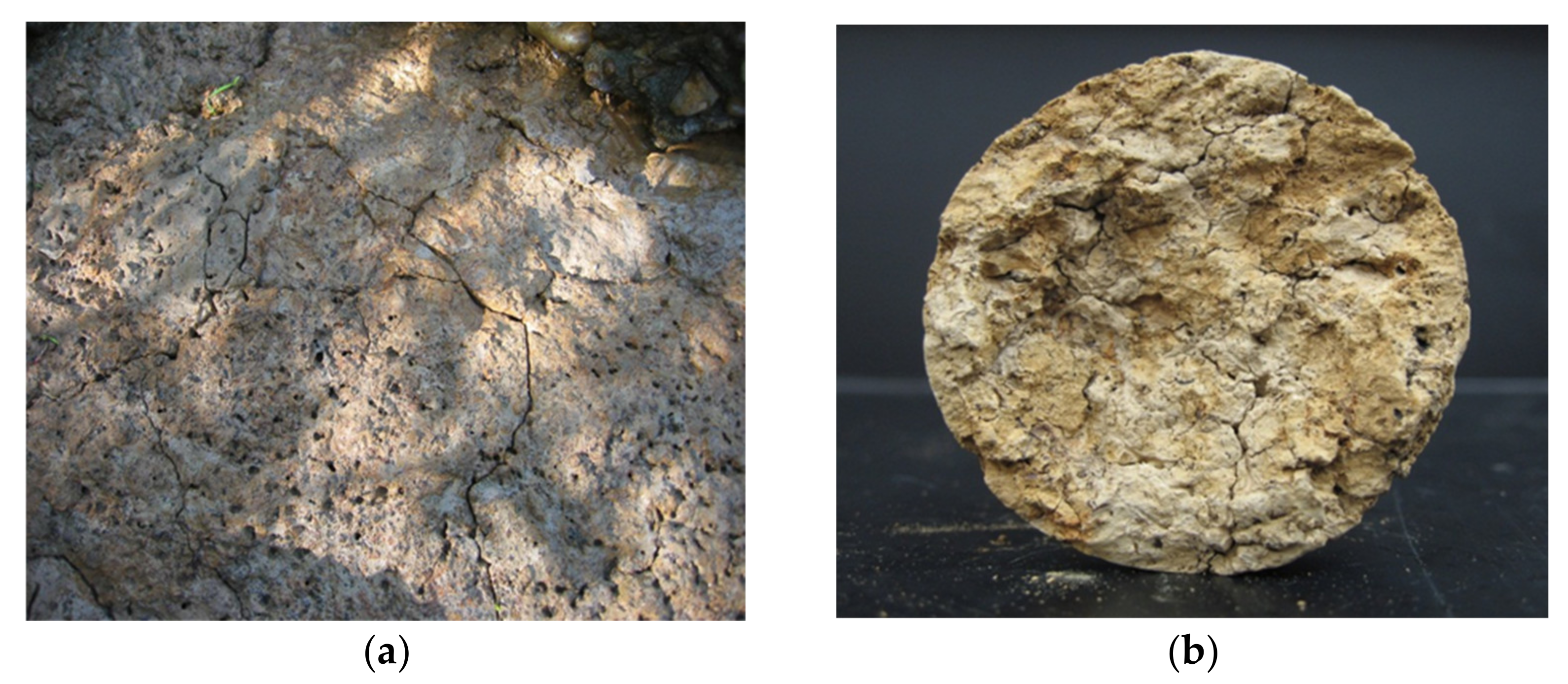
It was noticed that when an exposed surface of the fine-grained soils was submerged, it became sticky and slippery. Once the surface dried, however, superficial cracks developed, and the soil became hard and brittle. Although no distinct soil layers were apparent in the riverbank, chunks of soil fell off easily when dry, indicating pre-developed small-scale structured layers. As shown in Figure 3, the silt and clay soils in the field contain pores, cracks, and aggregates that may lead to the development of randomly structured soil characteristics.
2.2. Determination of Hydraulic Conductivity
Hydraulic conductivity (k) is the primary parameter to identify the flow characteristics of soils. It describes and predicts the flow magnitude and direction in the soil matrix. Due to the different degrees of resolution in available experimental methods and soil types, caution is needed to select and apply a technique. This caution is especially true with fine-grained soils, where extra care is necessary to estimate an expected value of hydraulic conductivity. Even though all the employed methods are known to provide saturated hydraulic conductivity, the actual test conditions and assumptions are different. Thus, the measured values may show a large discrepancy. Each adopted test is introduced below with its background and setup in the study.
2.2.1. Constant Head Permeability Test
The most common laboratory permeability test methods are the constant head permeability (CHP) and the falling head permeability (FHP) tests. In general, the CHP test is better suited for granular soils, while the FHP test is preferred for fine-grained soils due to the its ability to measure smaller flows. However, the CHP test can also be applied to finer soils using a Mariotte bottle or by superimposing a constant pressure in which the testing time is reduced by increasing the flow rate [15]. However, this must be performed cautiously because high pressure can initiate fractures in the soil sample, resulting in incorrect values of hydraulic conductivity.
In this study, the CHP tests with a constant air pressure were conducted using Tempe cells. The cell diameter was 5 cm, and the thickness of each sample was about 1 cm. An initial pressure below 5 kPa was applied to drain water in the system. Then the pressure was gradually increased to either 20 or 40 kPa and maintained until the drainage rate reached equilibrium. The hydraulic conductivity by the CHP kCHP is determined using the Equation (1):
where Q = flow rate, d = sample thickness, P = applied pressure head, and A = cross-sectional area of soil sample. The pressure head was increased in stages, and the results compared to confirm the hydraulic conductivity remained constant to check for the development of fractures during the test.
2.2.2. Oedometer Test
The oedometer test is the most widely used test for the one-dimensional consolidation of soils. As explained in the American Society for Testing and Materials (ASTM) standard [16], a constant vertical load is applied to the sample, and a time-deformation curve is plotted. After a series of oedometer tests, steadily increasing the constant load for each test, the primary consolidation under each loading is determined. The results are plotted in a void ratio e vs. log (p’) curve, where p’ is the effective vertical stress. Terzaghi [17] proposed an equation that can be used to determine hydraulic conductivity from the oedometer test. The hydraulic conductivity by the consolidation test kCON can be calculated from the Equation (2):
where = coefficient of consolidation, = coefficient of volume change, and = unit weight of water. The coefficient of volume change mv is determined from the slope of the e vs. log (p’) curve. The consolidation test provides hydraulic conductivity values k as a function of the void ratio e, which can be used to establish e vs. k relationships for the tested soil samples. Undisturbed specimens for the consolidation tests were trimmed from the Shelby tube and block soil samples. Each specimen’s typical size was about 63.5 mm in diameter with a thickness of about 20 mm. A vertical load of 10 kPa was applied initially and increased up to 760 kPa for each test.
2.2.3. Auger Hole Method
Due to the drawbacks of laboratory tests, including sample disturbance and the inability to precisely reproduce field conditions, in situ tests performed in the field are often preferred. The auger hole (AH) method is a quick and simple test that does not require sophisticated equipment and can be easily performed in the field when the water table is shallow. It was proposed by Diserens [18] and later improved by many researchers [19]. Additional benefits of the test are (i) the soil profile can be identified during the test, (ii) disturbed and undisturbed soil samples can be collected while drilling the holes, and (iii) several tests can be performed simultaneously.
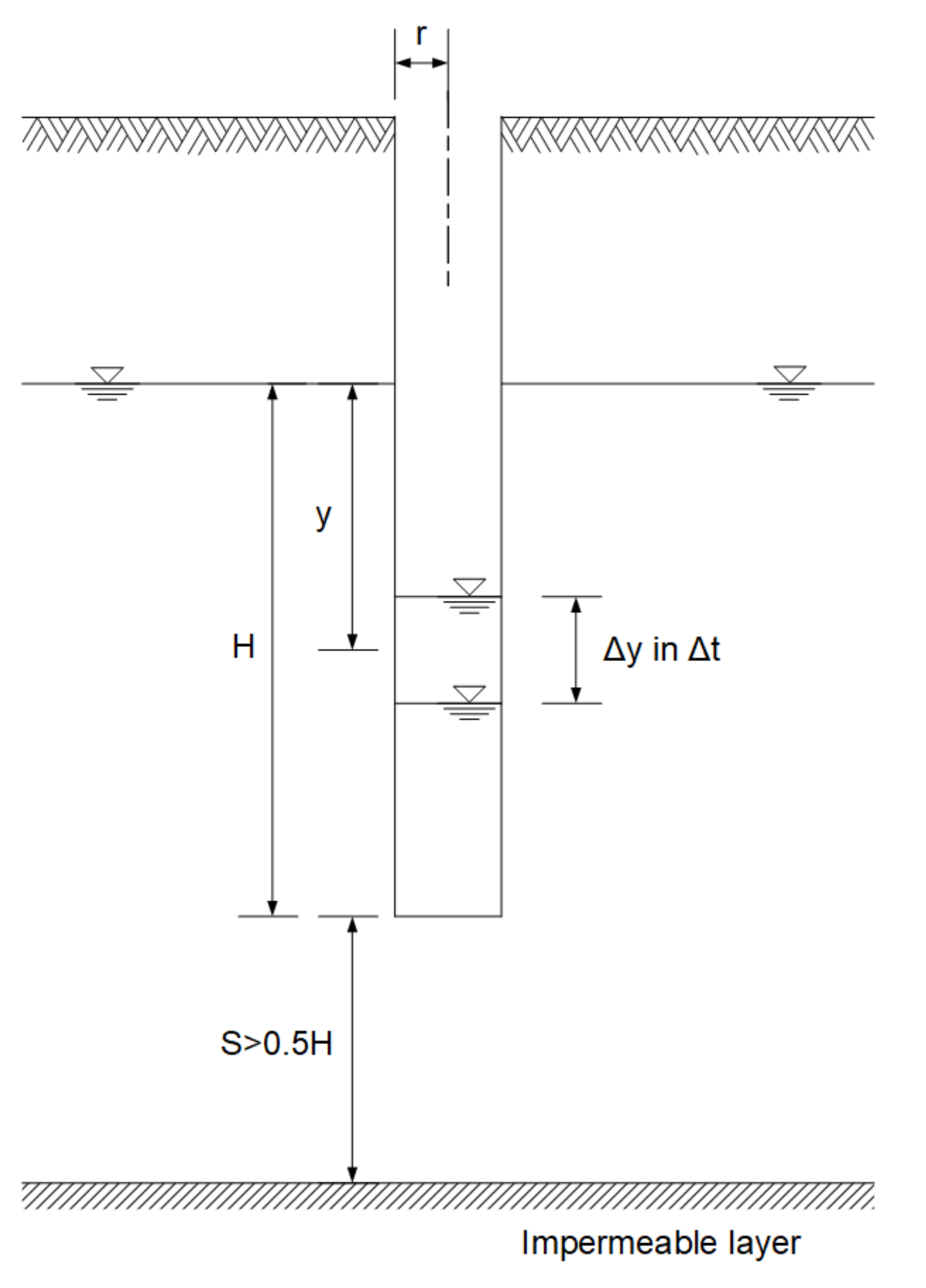
The auger hole method requires monitoring wells to be drilled that extend below the groundwater table. Once the observation well is completed and the water table inside the well reaches equilibrium, the test starts by removing the water in the hole. Groundwater then seeps into the hole, rising until it returns to the original level, and the time required to reach equilibrium is measured. As shown in Figure 4, the main parameters needed when conducting an auger hole test are the hole dimensions (radius r, depth h + H), the location of the water table in the hole (h), and the location of the impermeable layer below the hole (S). As van Beers [19] described, the results of an auger hole test can be interpreted using plots developed by Boumans [20] or by applying an equation first proposed by Ernst [21]. Although the graphical method is more accurate, the Equation (3) is preferable when the plots are not readily available [19]. The following Equation determined hydraulic conductivity by the auger hole test kAH for homogeneous soil with an impermeable layer existing 0.5 H or more below the bottom of the auger hole (S > 0.5H) [21]:
where r = radius of the hole, H = depth of the hole below the groundwater table, y = distance between the groundwater table and the average water level in the hole for a given time , = water level change in the hole for a given time , and S = distance from the bottom of the hole to the impermeable layer.
The variables in the above equation are defined in Figure 4, and the unit for kAH is m/day even though the input parameters are all in cm or second. Fourteen AH tests in total were performed at three different riverbank sites. As the tests need to be conducted below the water table, 13 measuring holes were made with a hand augur (10 cm in diameter), and one hole was made with a Shelby tube (7.5 cm in diameter). The depth of each auger hole varied from 0.6 to 1.2 m, and the volume of water withdrawn from the holes was also different due to the prevailing field conditions.
The Guelph permeameter (GP) method is an in situ constant head test that measures unsaturated soils’ saturated hydraulic conductivity using a Mariotte siphon reservoir. The rate at which water flows out of a cylindrical well above the groundwater table is measured, assuming that the soils around the well are homogeneous and saturated during the test. However, due to the saturation process in soils above the GWT, GP measurements are smaller than the actual saturated hydraulic conductivity [22]. Moreover, factors such as the soil’s initial water content and smearing and compaction of well walls affect the results significantly [23]. Thus, each hole in this study was finished with a well preparation brush to remove any smeared layer. Five GP tests were performed at three different riverbanks.
Interpretation of the test results can be made with one- or two-point measurements [24]. Although two-point measurements provide a better estimate of α*, the ratio of saturated hydraulic conductivity k to matric flux potential , measurements of one steady flow rate with a single ponded head, in which the hydraulic conductivity can be obtained using Equation (4), is known to be sufficient for estimating hydraulic conductivity [24].
where Q = steady intake rate of water, Hw = well height, r = well radius, = ratio of ksat to , and C = dimensionless shape factor =.
2.3. Groundwater Table Monitoring
When modeling transient seepage, the phreatic surface’s location is required as an initial boundary condition and, subsequently, may have a significant effect on modeling results. Model predictions for changes in the phreatic surface can be compared to observed GWT locations in the field. When the water surface elevation (WSE) in the river changes considerably with time, as may be the case during the passing of a flood, the predicted modeling results are strongly dependent on the values used for the hydraulic conductivity of the riverbank soils [31]. Thus, field observations of the groundwater table (GWT) can validate the hydraulic conductivity and, consequently, the modeling results.
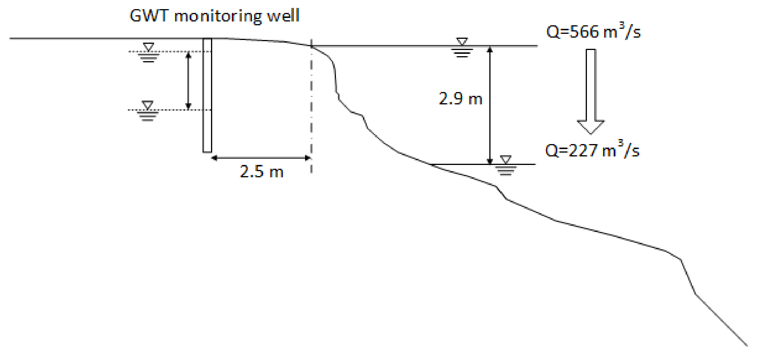
A groundwater table monitoring well was drilled to a depth of 3.2 m on the riverbank at site 1 using a hand drill, as shown in Figure 5. One GWT sensor was installed at the bottom of the monitoring well, and another pressure sensor was installed in the river. These two sensors simultaneously monitored changes in the WSE and the corresponding GWT.
The GWT sensors were built based on the design developed initially by Dedrick et al. [32] and upgraded by Riley et al. [33]. The device consists of a differential pressure sensor and a logger with a 12-bit microcontroller. The pressure sensor measures differential pressures between atmospheric and water pressures. The logger with the microcontroller digitizes an analog voltage from the sensor, and the data are stored in the memory. The measurement period is determined by battery life. Lithium batteries were used, allowing the sensor to operate continuously for several months. The resolution of the data logger is generally determined by the capacity of the sensor and microcontroller. The maximum measurable depth of water was 10 m, and the resolution of the sensor was set to 2.57 mm.
3. Transient Seepage Analysis
The main objective of transient seepage analysis was to compare the groundwater table observed in the monitoring well with the location of the phreatic surface predicted by the seepage modeling using hydraulic conductivities measured by the different methods. By comparing the modeling results and observations, the hydraulic conductivity values that produced the closest agreement can be determined.
When locating the GWT using transient seepage analysis, a complicating factor is the need to account for unsaturated soil conditions above the GWT. For unsaturated soils, the hydraulic conductivity is a function of saturation or soil water content, and seepage is strongly affected by matric suction. Strictly, modeling of unsaturated seepage requires two-phase fluid flow formulation with relative permeability and suction vs. saturation functions. Determination of these relationships is cumbersome and time-consuming.
On the other hand, the hydraulic conductivity function can be estimated from the saturated hydraulic conductivity and soil-water characteristic curve (SWCC) as an alternative, which relates the matric suction with saturation. Several methods have been suggested for this estimation, among which the methods proposed by Green and Corey [34], van Genuchten [35], and Fredlund et al. [36] are widely used [37].
3.1. Governing Equation
Darcy’s law can be applied to water flow through unsaturated soils using Richards equation [38]. The governing differential equation for the flow in unsaturated soils is also based on Darcy’s law for saturated soils and can be stated as follows [39]:
where h = total hydraulic head, kx, ky, and kz = hydraulic conductivity in the x, y, and z directions, respectively, q = external boundary flux, and = volumetric water content. Equation (5) describes the conservation of fluid mass in soils and states that the sum of the rates of flow changes in the x, y, and z directions and the external boundary flux are equal to the rate of change of volumetric water content per unit time [40].
Assuming that the total stress is constant and the air phase is continuous in the unsaturated soils, the change of volumetric water content can be simplified to Equation (6) [39]:
where uw = pore water pressure, mw = slope of the SWCC.
The governing equation for two-dimensional flows is then expressed as Equation (7):
In partially saturated soils, the hydraulic conductivity decreases as there is less cross-sectional area through which water can flow. It is known to be the function of matric suction, which can also be expressed in volumetric water content or degree of saturation.
In MIDAS GTS [41], a couple of options to define the relationships between the matric suction and relative hydraulic conductivity are available. The van Genuchten model is one of the available options that define the hydraulic conductivity function for negative pressure head (matric suction) with curve fitting parameters m and n [41]:
where is the calculated relative hydraulic conductivity; h is the negative pressure head; and a, n, and m are the curve fitting parameters, whereby a is related to the air entry suction head, 𝑛 corresponds to the soil pore size distribution, and m is set equal to 1 − 1/n.
3.2. Modeling Parameters
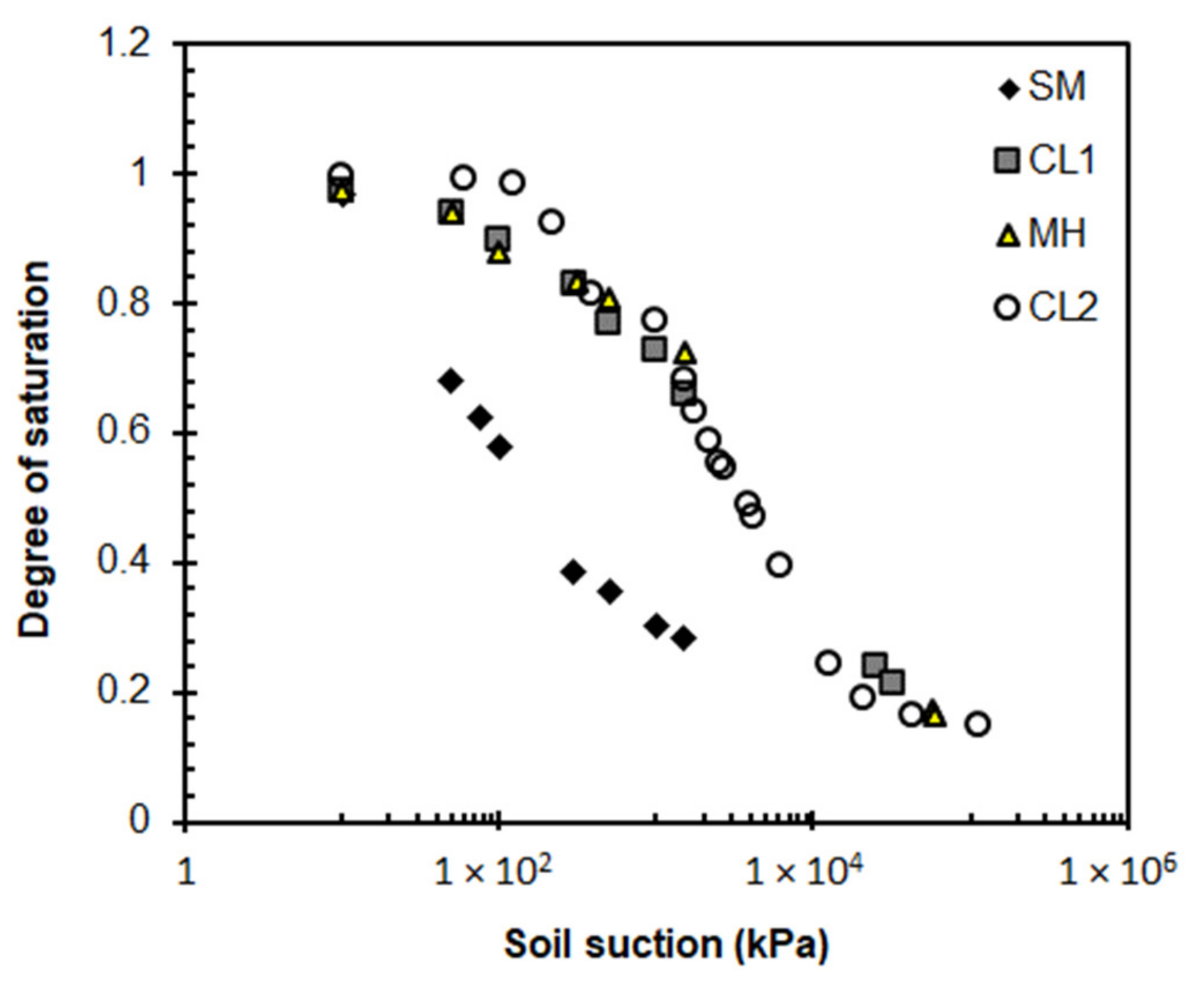
The SWCC in each soil layer at the field sites was determined using a combination of Tempe cell tests, pressure plate tests, filter paper tests, and a chilled mirror hygrometer. The results are presented as a group of data points that construct a continuous SWCC using van Genuchten’s model for each soil, as shown in Figure 6. Further details of obtaining the SWCC for the soil deposits in the lower Roanoke River are described in Nam et al. [37]. The SWCCs shown in Figure 6 are used to determine the slope mw required in Equation (7):
The transient seepage analysis is performed using the finite element program MIDAS GTS developed by MIDAS IT Co. Ltd. [42]. Average values of the additional modeling parameters used for the analysis are provided in Table 2. In this study, the measured soil suction values and corresponding volumetric water contents were directly entered into the program. The program finds the relative hydraulic conductivity and the curve-fitting parameters.
3.3. Riverbank Geometry and Soil Profile
Riverbank geometry was determined by the ground-based light detection and ranging (LiDAR) above the water surface and acoustic Doppler current profiler (ADCP) below [43]. The soil profile at each riverbank was established by visual observation and in situ tests in the field and laboratory tests using soil samples obtained from vertical auger holes. The hand auger was capable of drilling to depths of up to about 3 m. By drilling at several locations along the bank slope, the soil profile was identified to a depth of 6 m. Given that soil layers deeper than 6 m from the bank top could not be visually identified even during low flow, the thickness of the lowest soil layer below 6 m was assumed based on previous reports in the literature [13,14]. The riverbanks’ vertical soil profile was simplified using between three and five soil layers, including the assumed bottom impervious layer for modeling purposes.
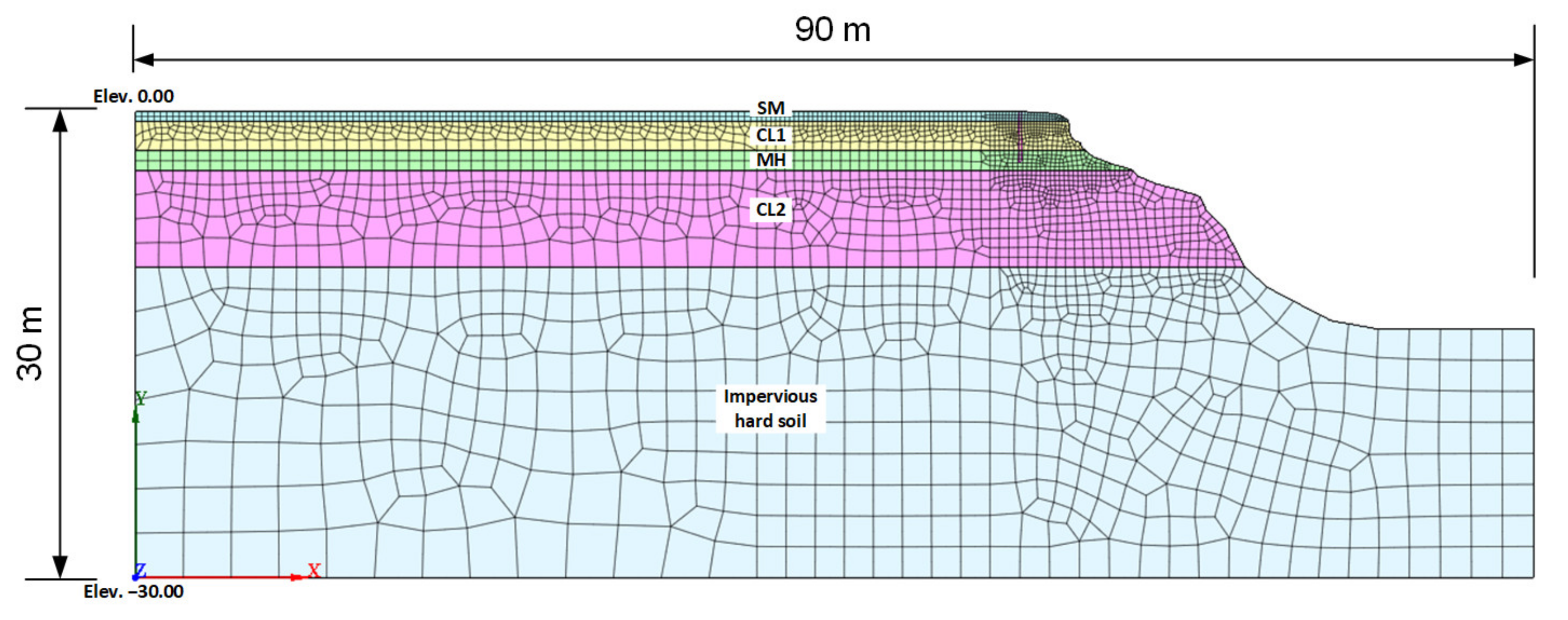
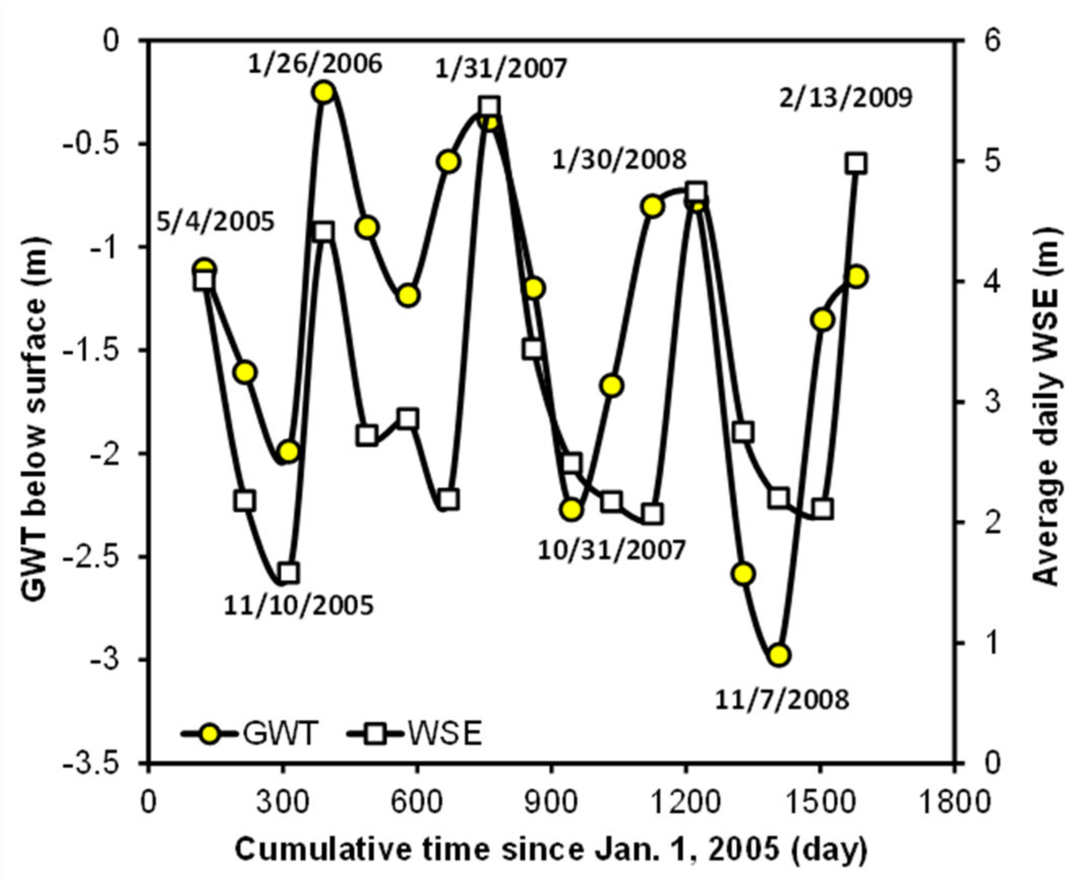
The transient seepage analysis was performed at site 1 on the outer bank of a meander bend—a location where the GWT was monitored. Figure 7 shows the riverbank geometry used for the seepage modeling. The model’s width and height are 90 and 30 m, respectively, following the ratio suggested by Desai [44], and the meshes were generated with 8-node quadrilateral elements. As for the boundary conditions, the water head is allowed to change freely on the right side of the model, while the left side is assumed to be the constant head boundary. The left boundary is set far enough from the well not to affect the prediction of the GWT. Laboratory tests and in situ tests with a few exceptions determined the input parameters for each soil layer, such as k, SWCC, and water content at saturation. The parameters kGP and kAH were assumed for the SM layer because the tests were not applicable due to high hydraulic conductivity. The long-term GWT observation data at the closest GWT monitoring station by the North Carolina Department of Environmental and Natural Resources (NC DENR) Division of Water Resources (Station no. F22B7, latitude 36.24° N, longitude 77.19° W) were analyzed, as shown in Figure 8. The GWT log overlapped the daily average WSE near the site during the same period, indicating that both the local groundwater and river elevations fluctuate regularly on a seasonal basis. Based on this observation, the initial location of the GWT for the numerical modeling was determined.
4. Result and Discussion
4.1. Comparison of Hydraulic Conductivities
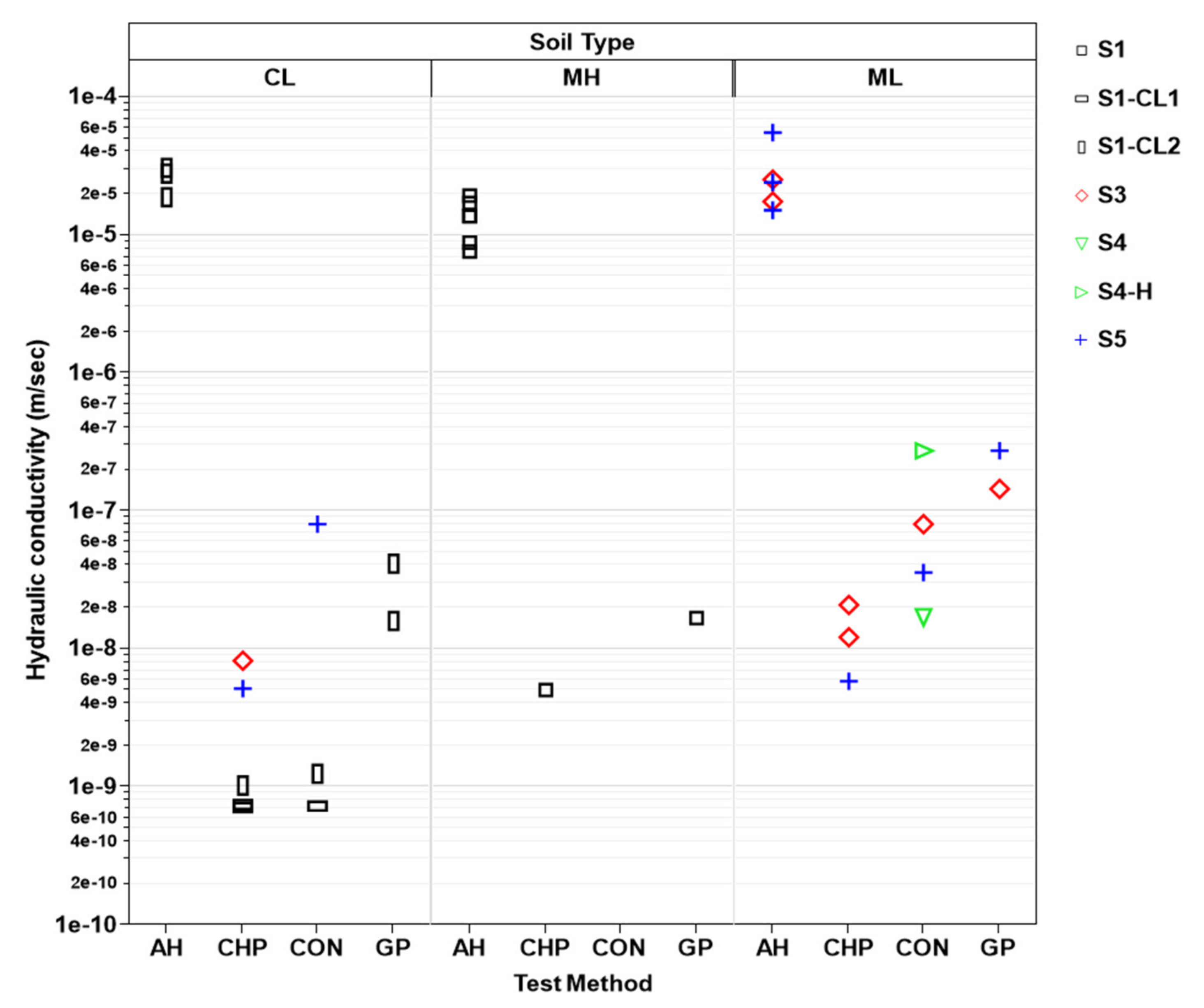
Hydraulic conductivity of the soils k at four different riverbanks was estimated using 35 laboratory and in situ tests, as shown in Figure 9. The estimated hydraulic conductivities were compared by soil types, test methods, and sampling/measuring locations. The hydraulic conductivity of the saturated clay soil (CL) varies from 10−9 to 10−5 m/s. The two silty soils, ML and MH, show similar ranges between 10−8 and 10−5 m/s. However, the differences in the hydraulic conductivity between each soil type (CL, MH, and ML) are much smaller than that between test methods (AH, CHP, CON, and GP). Similar trends were observed for the sampling locations, indicating that the differences amongst locations (sites 1, 3, 4, and 5) are relatively negligible between the test methods (AH, CHP, CON, and GP). Thus, these wide ranges for hydraulic conductivity seem to be attributable mainly to the different test methods. The soil types and sampling locations seem to be relatively insignificant in the saturated hydraulic conductivity estimation for the conditions encountered on the lower Roanoke River.
The auger hole method (AH) resulted in the highest hydraulic conductivity values—close to 10−5 m/s—followed by the Guelph permeameter test (GP) with values of around 10−7 m/s. The two laboratory methods, the constant head permeability test (CHP) and the consolidation test (CON), yielded lower values of around 10−9 m/s. The two laboratory methods resulted in similar values, whereas the difference between the two in situ methods was about two to three orders of magnitude.
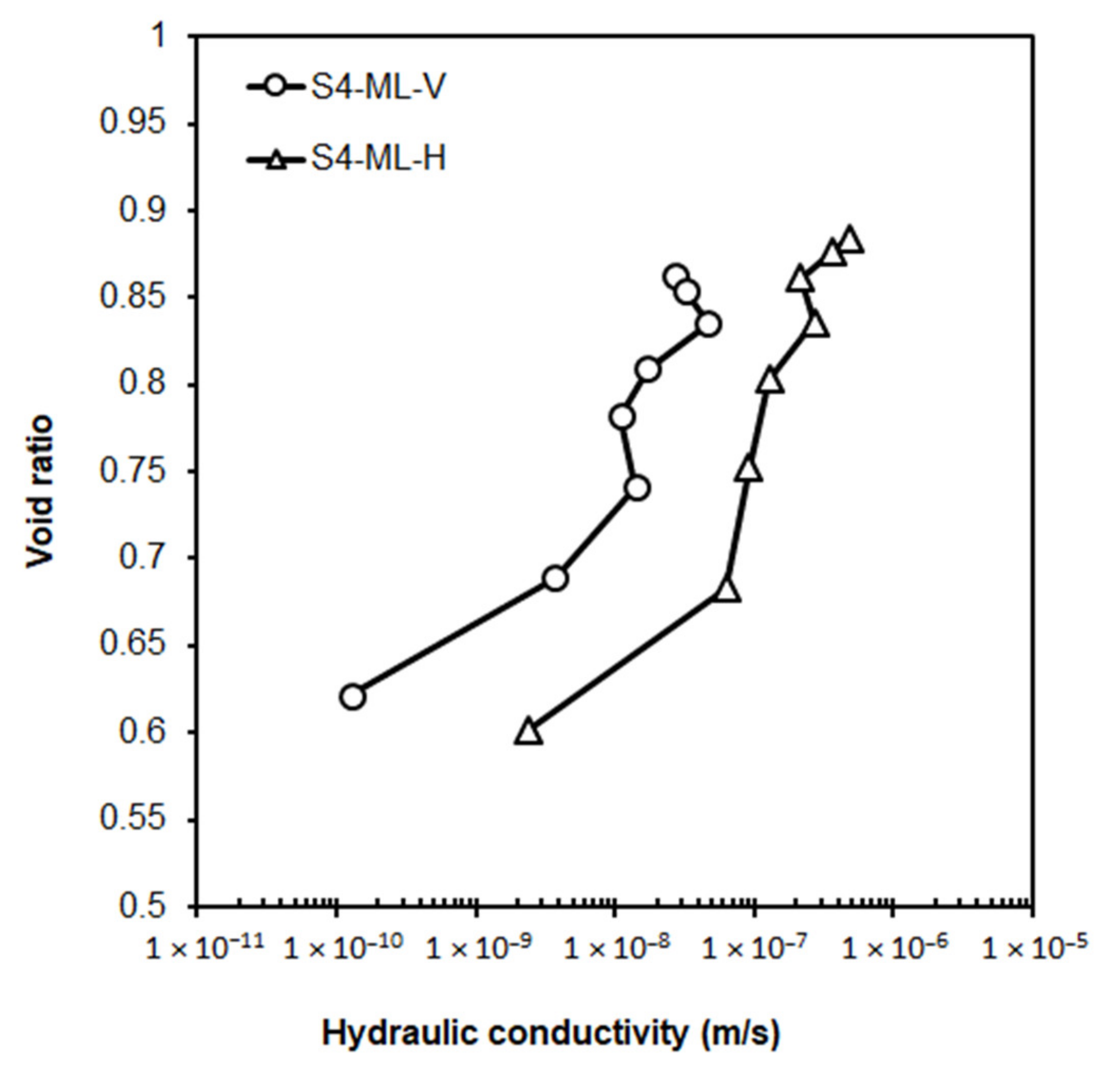
Samples from site 4 were trimmed perpendicular and parallel to the bedding plane and tested for the anisotropic hydraulic characteristic using the consolidation test (CON). The results, shown in Figure 10, revealed that the horizontal k was up to 20 times larger than the vertical k. The implications of anisotropic permeability on the test results are discussed in detail below.
4.2. Seepage Analysis
The laboratory and in situ experimental methods used to determine k produced a wide range of values. Thus, selecting an appropriate value for transient seepage analysis is difficult given the influence of k on the numerical results’ accuracy and reliability. Using values from the lower and upper bounds of the range will generate different results for the transient seepage analysis in terms of the predicted pore water pressure distribution and phreatic surface location. A numerical method to back-calculate field measurements of the GWT was employed to validate the model k-values. Transient seepage analysis was performed using MIDAS GTS [42] with different k-values from laboratory and in situ tests while keeping geometry, boundary conditions, and other soil parameters constant. Calculated changes of the phreatic surface with different river water elevations were then compared to the measured groundwater table from the monitoring wells to evaluate the various test methods.
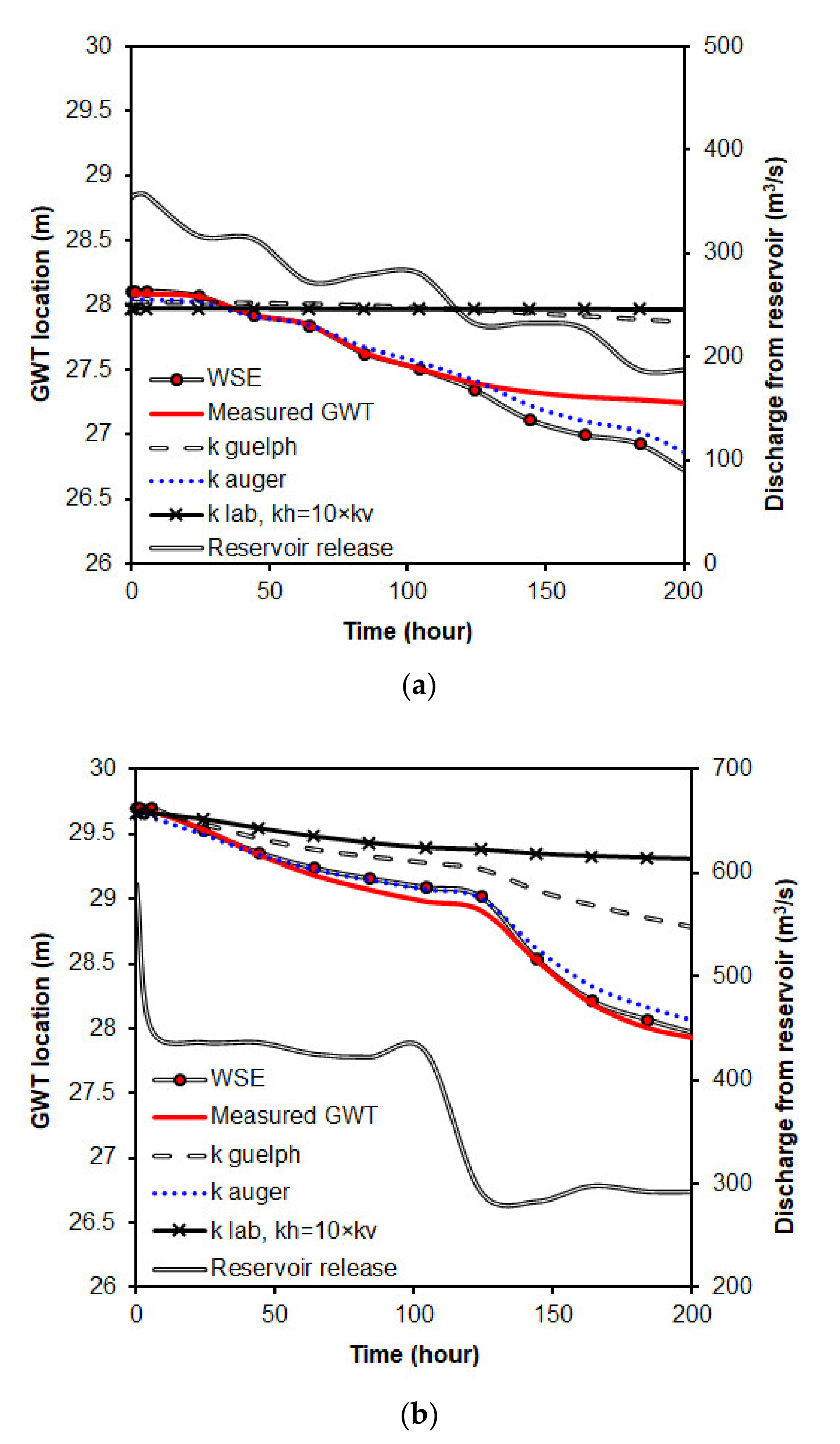
Two reservoir release events at site 1 were considered to fit the numerical models with the different k and monitored GWT. As shown in Figure 11, one event was observed between 23 and 31 May 2008, with the discharge varying from 354 to 187 m3/s through three stepped-down stages. The second event occurred between 20 and 29 June 2009, with the discharge changing from 589 to 292 m3/s in a single step.
The observed and estimated GWT and WSE corresponding to the reservoir releases using different hydraulic conductivities are presented in Figure 11. Klab is the horizontal hydraulic conductivity that is assumed to be 10 times larger than the vertical hydraulic conductivity. This figure demonstrates that the GWT responds almost instantly to the changes in the WSE. The results indicate that the highest k from AH produced the best agreement with the observed changes in the GWT. The difference between the observed GWT and the modeling result using the AH values could be due to the uncertainty associated with estimating the modeling parameters and boundary conditions in the seepage analysis. Considering the multiple orders of magnitude variations in the permeability values, the comparison between numerical modeling results and GWTs monitored in the field supports the validity and utility of in situ hydraulic conductivity measurements.
4.3. Discussion of Factors Affecting Hydraulic Conductivity
The numerical results produced the closest agreement to observations using the hydraulic conductivity from the auger hole method, kAH. It is unclear why kAH is higher than typical values for similar soil types and why significant differences are seen between in situ and laboratory values. Interestingly, each laboratory test produces similar results regardless of soil type and location. Thus, it is essential to identify the potential factors that contribute to this range of values to select the appropriate method to properly determine permeability values.
- (1)
- Test environment—The values for k from the in situ tests were higher than those from the lab tests. Of the two in situ tests, the AH method consistently produced higher values than the GP test. Weber [8] reported field to laboratory permeability ratios kF/kL for silty clay and sandy silty clay that were as high as 4,900 and 46,000, respectively. Reynolds and Zebchuk [45] also observed higher k-values with the AH method than with the GP in clay soil. Dorsey et al. [29] and Gallichand et al. [27] reported that the AH results in their study produced k-values that were about 1.4 to 83.3 times higher than the GP method. This difference was attributed to the test environment as the GP is performed after saturating soils near the bottom of the test hole but above the GWT. In contrast, the AH is performed in saturated soils below the GWT. Thus, the GP measures field-saturated hydraulic conductivity, which is smaller than the fully saturated hydraulic conductivity below the GWT. Although the soil is assumed to be saturated during the GP tests, air may be entrapped during the saturation process, resulting in a lower value for hydraulic conductivity than that for fully saturated hydraulic conductivity [46,47]. This situation is further complicated by the presence of inhomogeneous soil and pore conditions. While other studies have found that the entrapped air reduces the hydraulic conductivity, the magnitude of the reduction has been found to range from a factor of 2 to 5 [48,49] to up to 1 to 2 orders of magnitude [50,51].
- (2)
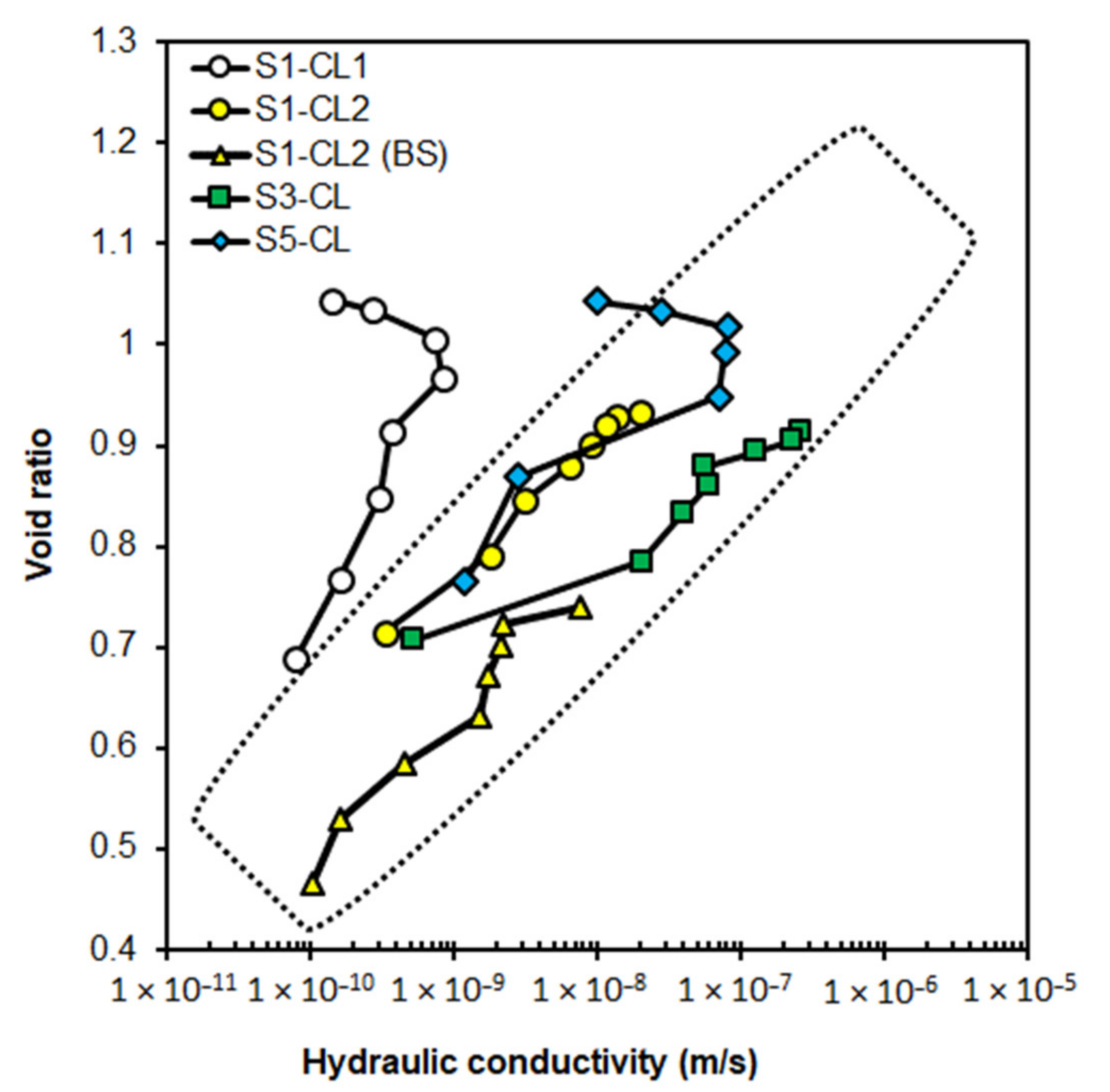
- Sample disturbance—In general, the logarithm of hydraulic conductivity is expected to decrease proportionally with a decrease in void ratio. However, the opposite trend was observed in some of the consolidation test results (see Figure 12), whereby the hydraulic conductivity initially increased as the void ratio is decreased. The e vs. log(k) curve follows the expected trend for void ratios below 1.0, but above this value, the logarithm of hydraulic conductivity increased as the void ratio is decreased. This trend could be due to sample disturbance resulting from the removal of the sample and transportation. Sample disturbance alters the fabric or structure of the samples (e.g., by creating discontinuities) in such a way as to increase hydraulic conductivity. The effects of sampling disturbance appear to diminish after the soil has been consolidated to a void ratio lower than 1.0.
Figure 12 also shows that the test results create a relatively narrow band of e vs. log(k) data for the same soil types shown in the dotted area. This band can be used to determine the in situ hydraulic conductivity from the experimental data if the in situ void ratio is known. In general, the field void ratios are more significant than the corresponding values in the lab for stress levels below the pre-consolidation stress [52]. Thus, the actual hydraulic conductivity for undisturbed soil samples is expected to be higher than the values determined in the laboratory.
- (3)
- Soil anisotropy—As shown in Figure 10, the results of consolidation tests on the horizontally and vertically trimmed soil samples indicate a horizontal hydraulic conductivity that is about 20 times larger than the vertical value. Although there was only one set of tests performed to examine the anisotropic characteristic of hydraulic conductivity, the finding that the horizontal k (kh) was more significant than the vertical k (kv) is consistent with previous reports for alluvial soils, i.e., [53,54]. The higher horizontal k can be attributed to bedding plane cracks and anisotropic depositional structure in riverbank soils [55]. According to Wu et al. [56] and Casagrande and Poulos [57], the ratio of horizontal to vertical permeability kh/kv for fine-grained soils was found to be on the order of 15 and 40. On the other hand, Mitchell and Soga [58] provide several references (e.g., [59,60,61,62]) indicating that this ratio varies but remains less than 10. While the riverbank soils on the lower Roanoke River exhibit anisotropy in hydraulic conductivity within the range of previous studies, further work is needed to clarify the role of soil properties and fluvial processes, such as erosion and deposition, on the in situ anisotropy.
- (4)
- Preferential flows—The k-values determined by in situ tests, while supported by observed changes in the GWT, still seem to be larger than typical hydraulic conductivity values for clay or silt. Similar observations at a natural levee in the Atchafalaya River Basin, LA, were reported by Newman [63]. Childs et al. [64] reported the much higher field k and anisotropy for clay soils and observed strictures and fissures in the soils. Jarvis and Messing [65] observed higher k in loam soils than in sandy soil but attributed this to the macrostructure induced by earthworms, plant roots, and shrinkage. Hydraulic conductivities in clay are known to be about 10 to 100 times different depending on its structures affected by cracks or bio-pores [66]. High hydraulic conductivities in fine-grained soils have been described using various terms. Among these methods are preferential flow, bypass flow, macropore drainage, or small-scale channeling flow. The definition of each term may vary somewhat, but all are commonly used to explain unusually high water flow rates in silt and clay soils. As Figure 3 shows, surface cracks and pores were observed in the field, serving as visual indicators of preferential flow paths. Beven and Germann [67] suggested that soil fauna, plant roots, cracks and fissures, and natural soil pipes contribute to the creation of macropores. They also considered that drought conditions would cause clay soil to crack, possibly to a considerable depth, and subsequent soil freezing and frost heave would also deepen soil cracks. In addition, Regalado and Munoz-Carpena [68] pointed out that due to natural conditions in the field, in situ test results are spatially variable due to small-scale heterogeneities such as in structure, texture, flora, fauna, and soil composition. Although there was no analysis of preferential flows for this study, it seems likely that preferential flow is the primary factor responsible for the rapid response of the GWT in fine-grained structured riverbank soils.
5. Conclusions
The hydraulic conductivity of silty sand, silt, and clay obtained from the lower Roanoke River’s riverbanks was determined using two laboratory tests and two field test methods. These tests are the constant head permeability test, the consolidation test, the Guelph permeameter, and the auger hole method. Numerical modeling of transient seepage using the resulting values for hydraulic conductivity was then performed to estimate different GWT locations for two different WSE drawdown scenarios. The results were compared with the observed GWT in the field.
The results revealed that the hydraulic conductivity from the auger hole method, kAH, was about 102 times larger than the hydraulic conductivity from the Guelph permeameter, kGP, and up to 104 times larger than the values measured from the constant head permeameter and oedometer tests (kCHP and kCON). Although kCHP and kCON were closer to the typically reported range of hydraulic conductivity for homogeneous clayey soils, the transient seepage analysis indicated the highest k value from the auger hole method. It produced the GWT prediction that best matched the observed GWT.
The more significant differences seem to be attributed to the heterogeneous soil conditions in the field. Roots, cracks, and structured soils were observed in the field, which could cause preferential flow. These factors were not quantitatively analyzed but are known to affect the in situ hydraulic conductivity. Further analyses of the experimental results, in conjunction with findings reported in the literature, confirmed the natural variability of k and the variability between each method. The difference in the hydraulic conductivity between laboratory and in situ permeability tests can be attributed to anisotropy, sample size and disturbance, and test method, but indicate that variability due to soil type in the field was relatively small. It can also be assumed that the combined effect would be more significant than that of a single parameter.
While the wide range of k-values occurring in natural deposits are well documented, k also depends on the test methods. Thus, the determination of k for riverbanks with structured fine-grained soils needs to be performed with care as many in situ factors that accelerate seepage may exist in the field. When determining k, especially for non-homogeneous fine-grained soils commonly found on riverbanks, a single source of information may not adequately represent the soils’ actual hydraulic conductivity. Thus, it is recommended that additional information be considered, including visual investigation, the geological and geomorphological background of the site, and numerical modeling, to increase reliability. In addition, a comparison of long-term observations with results of numerical seepage is analysis is recommended.
Author Contributions
Conceptualization, P.D. and M.G.; Methodology, P.D., M.G., S.N., and J.P.; Formal analysis, S.N.; Investigation, S.N. and J.P.; Resources, S.N. and J.P.; Data curation: S.N.; Writing—original draft preparation, S.N.; Writing—review and editing, P.D., M.G., and J.P.; Visualization, S.N.; Supervision, P.D. and M.G.; Project administration, P.D. and M.G.; Funding acquisition, P.D. and M.G. All authors have read and agreed to the published version of the manuscript.
Funding
This research was funded by Dominion Energy and United States Army Corps of Engineers.
Institutional Review Board Statement
Not applicable.
Informed Consent Statement
Not applicable.
Data Availability Statement
The data presented in this study are available on request from the first author.
Acknowledgments
The authors acknowledge the support of the Edna Bailey Sussman Foundation and the Hydro Research Foundation.
Conflicts of Interest
The authors declare no conflict of interest.
References
- Maharjan, M.; Donovan, J.J. Groundwater response to serial stream stage fluctuations in shallow unconfined alluvial aquifers along a regulated stream (West Virginia, USA). Hydrogeol. J. 2016, 24, 2003–2015. [Google Scholar] [CrossRef]
- Nimmo, J.R.; Healy, R.W.; Stonestrom, D.A. Aquifer Recharge. In Encyclopedia of Hydrological Science; Anderson, M.G., Bear, J., Eds.; Wiley: Chichester, UK, 2005; Volume 4, pp. 2229–2246. [Google Scholar]
- Li, S.; Knappett, J.; Feng, X. Investigation of Slope Stability Influenced by Change of Reservoir Water Level in Three Gorges of China. In Proceedings of the Flow in Porous Media: From Phenomena to Engineering and Beyond: Conference Paper from 2009 International Forum on Porous Flow and Applications, Wuhan, China, 24–26 April 2009. [Google Scholar]
- Gofar, N.; Rahardjo, H. Saturated and unsaturated stability analysis of slope subjected to rainfall infiltration. MATEC Web Conf. 2017, 101, 05004. [Google Scholar] [CrossRef] [Green Version]
- Francisca, F.; Carro Pérez, M.; Glatstein, D.; Montoro, M. Contaminant transport and fluid flow in soils. In Horizons in Earth Research; Nova Science Publishers: New York, NY, USA, 2012; pp. 97–131. [Google Scholar]
- Derx, J.; Blaschke, A.P.; Farnleitner, A.H.; Pang, L.; Blöschl, G.; Schijven, J.F. Effects of fluctuations in river water level on virus removal by bank filtration and aquifer passage—A scenario analysis. J. Contam. Hydrol. 2013, 147, 34–44. [Google Scholar] [CrossRef]
- Vukovic, M.; Soro, A. Determination of Hydraulic Conductivity of Porous Media from Grain-Size Composition; Water Resources Publications: Littleton, CO, USA, 1992. [Google Scholar]
- Weber, W.G. In situ permeabilities for determining rates of consolidation. Highw. Res. Rec. 1968, 243, 49–61. [Google Scholar]
- Goodall, D.C.; Quigley, R.M. Pollutant migration from two sanitary landfill sites near Sarnia, Ontario. Can. Geotech. J. 1977, 14, 223–236. [Google Scholar] [CrossRef]
- Golder, H.Q.; Gass, A.A. Field Tests for Determining Permeability of Soil Strata; Brown, P., Shockley, W., Eds.; ASTM International: West Conshohocken, PA, USA, 1962; pp. 29–46. [Google Scholar] [CrossRef]
- Brown, P.M.; Miller, J.A.; Swain, F.M. Structural and Stratigraphic Framework and Spatial Distribution of Permeability of the Atlantic Coastal Plain, North Carolina to New York; U.S. Geological Survey: Reston, VA, USA, 1972; p. 79. [Google Scholar]
- Hupp, C.R.; Schenk, E.R.; Richter, J.M.; Peet, R.K.; Townsend, P.A. Bank erosion along the dam-regulated lower Roanoke River, North Carolina. Geol. Soc. Am. Spec. Pap. 2009, 451, 97–108. [Google Scholar] [CrossRef] [Green Version]
- Weems, R.E.; Lewis, W.C. Detailed Sections from Auger Holes in the Roanoke Rapids 1:100,000 Map Sheet, North Carolina; Open File Report 2007–1092; U.S. Geological Survey: Reston, VA, USA, 2007; p. 155. [Google Scholar]
- Weems, R.E.; Lewis, W.C.; Aleman-Gonzalez, W.B. Surficial Geologic Map of the Roanoke Rapids 30’× 60’ Quadrangle, North Carolina: U.S. Geological Survey Open-File Report 2009–1149, 1 Sheet, Scale 1:100,000; U.S. Geological Survey: Reston, VA, USA, 2009. [Google Scholar]
- Olson, R.E.; Daniel, D.E. Measurement of the hydraulic conductivity of fine-grained soils. In Permeability and Groundwater Contaminant Transport; ASTM STP 746; ASTM International: West Conshohocken, PA, USA, 1981; pp. 18–64. [Google Scholar] [CrossRef]
- ASTM D2435. Standard Test Methods for One-Dimensional Consolidation Properties of Soils Using Incremental Loading; ASTM International: West Conshohocken, PA, USA, 2004. [Google Scholar]
- Terzaghi, K. Theoretical Soil Mechanics; John Wiley and Sons: New York, NY, USA, 1943; p. 510. [Google Scholar]
- Diserens, E. Beitrag zur Bestimmung der Durchlässigkeit des Bodens in natürlicher Bodenlagerung. Schweiz. Landw. Mon. 1934, 12, 1–19. [Google Scholar]
- Van Beers, W.F.J. The Auger Hole Method: A Field Measurement of the Hydraulic Conductivity of Soil below the Water Table, 6th ed.; International Institute for Land Reclamation and Improvement: Wageningen, The Netherlands, 1983. [Google Scholar]
- Boumans, J.H. Het Bepalen van de Drainafstand Met Behulp van de Boorgaten Methode; Landbouwtijdschrift: The Hague, The Netherlands, 1953; pp. 82–104. [Google Scholar]
- Ernst, L.F. A New Formula for the Calculation of the Permeability Factor with the Auger Hole Method; Agricultural Experiment Station T.N.O.: Groningen, The Netherlands, 1950. [Google Scholar]
- Lee, D.M.; Reynolds, W.D.; Elrick, D.E.; Clothier, B.E. A comparison of three field methods for measuring saturated hydraulic conductivity. Can. J. Soil Sci. 1985, 65, 563–573. [Google Scholar] [CrossRef]
- Elrick, D.E.; Reynolds, W.D.; Tan, K.A. Hydraulic conductivity measurements in the unsaturated zone using improved well analyses. Ground Water Monit. Remediat. 1989, 9, 184–193. [Google Scholar] [CrossRef]
- Soilmoisture Equipment Corp. 2800K1 Guelph Permeameter Operating Instructions; Soilmoisture Equipment Corp: Goleta, CA, USA, 2006. [Google Scholar]
- Salverda, A.P.; Dane, J.H. An examination of the Guelph permeameter for measuring the soil’s hydraulic properties. Geoderma 1993, 57, 405–421. [Google Scholar] [CrossRef]
- Reynolds, W.D.; Elrick, D.E. In situ measurement of field-saturated hydraulic conductivity, sorptivity and the a-parameter using the Guelph permeameter. Soil Sci. 1985, 140, 292–302. [Google Scholar] [CrossRef]
- Gallichand, J.; Madramootoo, C.A.; Enright, P.; Barrington, S.F. An evaluation of the Guelph permeameter for measuring saturated hydraulic conductivity. Trans. Am. Soc. Agric. Eng. 1990, 33, 1179–1184. [Google Scholar] [CrossRef]
- Elrick, D.E.; Reynolds, W.D.; Lee, D.M.; Clothier, B.E. The “Guelph Permeameter” for measuring the field-saturated soil hydraulic conductivity above the water table: I. Theory, procedures and applications. In Proceedings of the Canadian Hydrology Symposium, Quebec City, QC, Canada, 10–12 June 1984; pp. 643–655. [Google Scholar]
- Dorsey, J.D.; Ward, A.D.; Fausey, N.R.; Bair, E.S. A comparison of four field methods for measuring saturated hydraulic conductivity. Trans. ASAE 1990, 33, 1925–1931. [Google Scholar] [CrossRef]
- Bagarello, V. Influence of well preparation on field-saturated hydraulic conductivity measured with the Guelph Permeameter. Geoderma 1997, 80, 169–180. [Google Scholar] [CrossRef]
- Wise, W.R.; Clement, T.P.; Molz, F.J. Variably saturated modeling of transient drainage: Sensitivity to soil properties. J. Hydrol. 1994, 161, 91–108. [Google Scholar] [CrossRef]
- Dedrick, R.R.; Halfman, J.D.; Brooks McKinney, D. An inexpensive, microprocessor-based, data logging system. Comput. Geosci. 2000, 26, 1059–1066. [Google Scholar] [CrossRef]
- Riley, T.C.; Endreny, T.A.; Halfman, J.D. Monitoring soil moisture and water table height with a low-cost data logger. Comput. Geosci. 2006, 32, 135–140. [Google Scholar] [CrossRef]
- Green, R.E.; Corey, J.C. Calculation of hydraulic conductivity: A further evaluation of some predictive methods. Soil Sci. Soc. Am. J. 1971, 35, 3–8. [Google Scholar] [CrossRef]
- Van Genuchten, M.T. A closed-form equation for predicting the hydraulic conductivity of unsaturated soils. Soil Sci. Soc. Am. J. 1980, 44, 892–898. [Google Scholar] [CrossRef] [Green Version]
- Fredlund, D.G.; Xing, A.; Huang, S. Predicting the permeability function for unsaturated soils using the soil-water characteristic curve. Can. Geotech. J. 1994, 31, 533–546. [Google Scholar] [CrossRef]
- Nam, S.; Gutierrez, M.; Diplas, P.; Petrie, J.; Wayllace, A.; Lu, N.; Munoz, J.J. Comparison of testing techniques and models for establishing the SWCC of riverbank soils. Eng. Geol. 2010, 110, 1–10. [Google Scholar] [CrossRef]
- Richards, L.A. Capillary conduction of liquids through porous mediums. Physics 1931, 1, 318–333. [Google Scholar] [CrossRef]
- Lam, L.; Fredlund, D.G.; Barbour, S.L. Transient seepage model for saturated-unsaturated soil systems: A geotechnical engineering approach. Can. Geotech. J. 1987, 24, 565–580. [Google Scholar] [CrossRef] [Green Version]
- Ng, C.W.W.; Shi, Q. A numerical investigation of the stability of unsaturated soil slopes subjected to transient seepage. Comput. Geotech. 1998, 22, 1–28. [Google Scholar] [CrossRef]
- MIDAS Information Technology Co. Ltd. GTS Analysis Reference; MIDAS Information Technology Co. Ltd.: Kyonggi-do, Korea, 2009. [Google Scholar]
- MIDAS Information Technology. Midas GTS, 4.1.0; MIDAS Information Technology: Seoul, Korea, 2010. [Google Scholar]
- Petrie, J.; Diplas, P.; Gutierrez, M.; Nam, S. Data evaluation for acoustic Doppler current profiler measurements obtained at fixed locations in a natural river. Water Resour. Res. 2013, 49, 1003–1016. [Google Scholar] [CrossRef]
- Desai, C.S. Finite element methods for flow in porous media. In Finite Elements in Fluids, Vol.1: Viscous Flows and Hydrodynamics; Wiley: Chichester, UK, 1975; pp. 157–182. [Google Scholar]
- Reynolds, W.D.; Zebchuk, W.D. Hydraulic conductivity in a clay soil: Two measurement techniques and spatial characterization. Soil Sci. Soc. Am. J. 1996, 60, 1679–1685. [Google Scholar] [CrossRef]
- Stephens, D.B.; Lambert, K.; Watson, D. Regression models for hydraulic conductivity and field test of the borehole permeameter. Water Resour. Res. 1987, 23, 2207–2214. [Google Scholar] [CrossRef]
- Reynolds, W.D.; Elrick, D.E.; Topp, G.C. A reexamination of the constant head well permeameter method for measuring saturated hydraulic conductivity above the water-table. Soil Sci. 1983, 136, 250–268. [Google Scholar] [CrossRef]
- Constantz, J.; Herkelrath, W.N.; Murphy, F. Air Encapsulation During Infiltration. Soil Sci. Soc. Am. J. 1988, 52, 10–16. [Google Scholar] [CrossRef]
- Stephens, D.B.; Lambert, K.; Watson, D. Influence of entrapped air on field determinations of hydraulic properties in the vadose zone. In Proceedings of the Conference on Characterization and Monitoring of the Vadose Zone, Las Vegas, NV, USA, 7–11 December 1983; pp. 57–76. [Google Scholar]
- Faybishenko, B. Comparison of laboratory and field methods for determining the quasi-saturated hydraulic conductivity of soils. In Proceedings of the 1997 Riverside International Workshop on Soil Hydraulic Properties, Riverside, CA, USA, 22–24 October 1997; pp. 279–292. [Google Scholar]
- Sakaguchi, A.; Nishimura, T.; Kato, M. The Effect of Entrapped Air on the Quasi-Saturated Soil Hydraulic Conductivity and Comparison with the Unsaturated Hydraulic Conductivity. Vadose Zone J. 2005, 4, 139–144. [Google Scholar] [CrossRef]
- Terzaghi, K.; Peck, R.B.; Mesri, G. Soil Mechanics in Engineering Practice, 3rd ed.; John Wiley & Sons: Hoboken, NJ, USA, 1996. [Google Scholar]
- Phonate, V.; Malik, R.S.; Kumar, S. Anisotropy in some alluvial soils. Ann. Arid Zone 2001, 40, 425–427. [Google Scholar]
- Chen, X.H. Streambed hydraulic conductivity for rivers in south-central Nebraska. J. Am. Water Resour. Assoc. 2004, 40, 561–573. [Google Scholar] [CrossRef]
- Rycroft, D.W.; Amer, M.H. Prospects for the Drainage of Clay Soils; Food and Agriculture Organization of the United Nations: Rome, Italy, 1995. [Google Scholar]
- Wu, T.H.; Chang, N.Y.; Ali, E.M. Consolidation and strength properties of a clay. J. Geotech. Eng. Div. Asce 1978, 104, 889–905. [Google Scholar] [CrossRef]
- Casagrande, L.; Poulos, S. On the effectiveness of sand drains. Can. Geotech. J. 1969, 6, 287–326. [Google Scholar] [CrossRef]
- Mitchell, J.K.; Soga, K. Fundamentals of Soil Behavior, 3rd ed.; John Wiley & Sons, Inc.: New York, NY, USA, 2005. [Google Scholar]
- Olsen, H.W. Hydraulic Flow Through Saturated Clays. Clays Clay Miner. 1962, 9, 131–161. [Google Scholar] [CrossRef]
- Chan, H.T.; Kenney, T.C. Laboratory Investigation of Permeability Ratio of New Liskeard Varved Soil. Can. Geotech. J. 1973, 10, 453–472. [Google Scholar] [CrossRef]
- Ladd, C.C.; Wissa, A.E.Z. Geology and Engineering Properties of Connecticut Valley Varved Clays with Special Reference to Embankment Construction; Department of Civl Engineering, Massachusetts Institute of Technology: Cambridge, MA, USA, 1970. [Google Scholar]
- Mitchell, J.F. The fabric of natural clays and its relation to engineering properties. In Proceedings of the Thirty-Fifth Annual Meeting of the Highway Research Board, Washington, DC, USA, 17–20 January 1956; pp. 693–713. [Google Scholar]
- Newman, A.E. Water and Solute Transport in the Shallow Subsurface of a Riverine Wetland Natural Levee; Louisiana State University: Baton Rouge, LA, USA, 2010. [Google Scholar]
- Childs, E.C.; Collis-George, N.; Holmes, J.W. Permeability measurements in the field as an assessment of anisotropy and structure development. Eur. J. Soil Sci. 1957, 8, 27–41. [Google Scholar] [CrossRef]
- Jarvis, N.J.; Messing, I. Near-saturated hydraulic conductivity in soils of contrasting texture measured by tension infiltrometers. Soil Sci. Soc. Am. J. 1995, 59, 27–34. [Google Scholar] [CrossRef]
- Vlotman, W.F.; Smedema, L.K.; Rycroft, D.W. Modern Land Drainage: Planning, Design and Management of Agricultural Drainage Systems, 2nd ed.; CRC Press/Balkema: Leiden, The Netherlands, 2020. [Google Scholar] [CrossRef]
- Beven, K.; Germann, P. Macropores and water flow in soils. Water Resour. Res. 1982, 18, 1311–1325. [Google Scholar] [CrossRef] [Green Version]
- Regalado, C.M.; Munoz-Carpena, R. Estimating the saturated hydraulic conductivity in a spatially variable soil with different permeameters: A stochastic Kozeny-Carman relation. Soil Tillage Res. 2004, 77, 189–202. [Google Scholar] [CrossRef]
Figure 1.
Field study site location showing (a) the United States and the location of the lower Roanoke River watershed in North Carolina; (b) the Roanoke River watershed below the Roanoke Rapids Dam; and (c) the study sites on the lower Roanoke River.
Figure 1.
Field study site location showing (a) the United States and the location of the lower Roanoke River watershed in North Carolina; (b) the Roanoke River watershed below the Roanoke Rapids Dam; and (c) the study sites on the lower Roanoke River.

Figure 2.
Atterberg limits of soils from the test sites (C: clay, M: silt, O: organic soil, H: high plasticity, and L: low plasticity).
Figure 2.
Atterberg limits of soils from the test sites (C: clay, M: silt, O: organic soil, H: high plasticity, and L: low plasticity).

Figure 3.
Evidence of structured soils: (a) surface condition of CL soil in the field, (b) small-scale structured layer on a dried sample.
Figure 3.
Evidence of structured soils: (a) surface condition of CL soil in the field, (b) small-scale structured layer on a dried sample.

Figure 4.
Schematic of the auger hole method. (r = radius of the hole, H = depth of the hole below the groundwater table, y = distance between the groundwater table and the average water level in the hole for a given time ∆t, ∆y = water level change in the hole for a given time ∆t, and S = distance from the bottom of the hole to the impermeable layer).

Figure 5.
Schematic of the groundwater table observation hole at site 1 with the change in WSE shown for an example drawdown event.
Figure 5.
Schematic of the groundwater table observation hole at site 1 with the change in WSE shown for an example drawdown event.

Figure 6.
Soil-water characteristic curve data for the four soil types found at the field sites.

Figure 7.
Bank geometry and finite element mesh for the transient seepage analysis.

Figure 8.
Variation of groundwater table and water surface elevation between 2005 and 2009.

Figure 9.
Hydraulic conductivity measured by different methods (AH = auger hole, CHP = constant head permeability, CON = consolidation test, GP = Guelph permeameter).
Figure 9.
Hydraulic conductivity measured by different methods (AH = auger hole, CHP = constant head permeability, CON = consolidation test, GP = Guelph permeameter).

Figure 10.
Influence of anisotropy and sampling method (V = vertical permeability and H = horizontal permeability).
Figure 10.
Influence of anisotropy and sampling method (V = vertical permeability and H = horizontal permeability).

Figure 11.
Changes in the GWT with hydraulic conductivity values determined from the field and laboratory tests for (a) 23–31 May 2008 and (b) 20–29 June 2009.
Figure 11.
Changes in the GWT with hydraulic conductivity values determined from the field and laboratory tests for (a) 23–31 May 2008 and (b) 20–29 June 2009.

Figure 12.
Results of the consolidation tests for CL soils from different locations.


Table 1.
Physical properties of riverbank soils on the lower Roanoke River.
| USCS Soil Type | Soil Properties | |||||
|---|---|---|---|---|---|---|
| Liquid Limit | Plasticity Index | Specific Gravity | Sand Content | Silt Content | Clay Content | |
| LL (%) | PI (%) | Gs | (%) | (%) | (%) | |
| SM | Non-Plastic | 2.69 | 69.5 | 22.0 | 8.5 | |
| CL | 41.6 | 18.3 | 2.72 | 16.9 | 50.1 | 33.0 |
| MH | 52.7 | 21.6 | 2.73 | 9.2 | 44.6 | 46.2 |
| ML | 41.2 | 13.7 | 2.72 | 25.4 | 48.2 | 26.4 |
Table 2.
Soil properties used in transient seepage analysis.
| Depth (m) | USCS Soil Type | kAuger (m/s) | kGuelph (m/s) | kLab (m/s) | Volumetric Water Content (%) |
|---|---|---|---|---|---|
| 0.0–0.6 | SM | 1.84 × 10⁻⁴ | 1.44 × 10⁻⁵ | 5.09 × 10⁻⁷ | 46.1 |
| 0.6–2.5 | CL | 2.64 × 10⁻⁵ | 2.08 × 10⁻⁸ | 7.32 × 10⁻¹⁰ | 50.3 |
| 2.5–3.8 | MH | 1.35 × 10⁻⁵ | 1.69 × 10⁻⁸ | 4.99 × 10⁻⁹ | 48.3 |
| 3.8–10.0 | CL | 2.58 × 10⁻⁵ | 1.86 × 10⁻⁸ | 1.02 × 10⁻⁹ | 47.8 |
| >10.0 | Impervious hard soil | 1.26 × 10⁻⁸ | 1.26 × 10⁻¹⁰ | 1.26 × 10⁻¹⁰ | 26.0 |
Publisher’s Note: MDPI stays neutral with regard to jurisdictional claims in published maps and institutional affiliations. |
© 2021 by the authors. Licensee MDPI, Basel, Switzerland. This article is an open access article distributed under the terms and conditions of the Creative Commons Attribution (CC BY) license (https://creativecommons.org/licenses/by/4.0/).
Share and Cite
MDPI and ACS Style
Nam, S.; Gutierrez, M.; Diplas, P.; Petrie, J. Laboratory and In Situ Determination of Hydraulic Conductivity and Their Validity in Transient Seepage Analysis. Water 2021, 13, 1131. https://doi.org/10.3390/w13081131
AMA Style
Nam S, Gutierrez M, Diplas P, Petrie J. Laboratory and In Situ Determination of Hydraulic Conductivity and Their Validity in Transient Seepage Analysis. Water. 2021; 13(8):1131. https://doi.org/10.3390/w13081131
Chicago/Turabian StyleNam, Soonkie, Marte Gutierrez, Panayiotis Diplas, and John Petrie. 2021. "Laboratory and In Situ Determination of Hydraulic Conductivity and Their Validity in Transient Seepage Analysis" Water 13, no. 8: 1131. https://doi.org/10.3390/w13081131
Note that from the first issue of 2016, this journal uses article numbers instead of page numbers. See further details here.