
A Unique Approach on How to Work Around the Common Uncertainties of Local Field Data in the PERSiST Hydrological Model


Department of Landscape Management, Faculty of Forestry and Wood Technology, Mendel University, Zemědělská 3, 613 00 Brno, Czech Republic
*
Author to whom correspondence should be addressed.
Water 2021, 13(9), 1143; https://doi.org/10.3390/w13091143
Submission received: 20 December 2020
/
Revised: 18 February 2021
/
Accepted: 26 February 2021
/
Published: 21 April 2021
(This article belongs to the Section Water Quality and Contamination)
Abstract
:In the last two decades, the effects of global climate change have caused a continuous drying out of temperate landscapes. One way in which drying out has manifested is as a visible decrease in the streamflow in the water recipients. This article aims to answer the questions of how severe this streamflow decrease is and what is its main cause. The article is based on the analysis of daily streamflow, temperature, and precipitation data during five years (1 November 2014 to 31 October 2019) in a spruce-dominated temperate upland catchment located in the Czech Republic. Streamflow values were modeled in the PERSiST hydrological model using precipitation and temperature values obtained from the observational E-OBS gridded dataset and calibrated against in situ measured discharge. Our modeling exercise results show that the trend of decreasing water amounts in forest streams was very significant in the five-year study period, as shown in the example of the experimental catchment Křtiny, where it reached over −65%. This trend is most likely caused by increasing temperature. An unexpected disproportion was found in the ratio of increasing temperature to decreasing discharge during the growing seasons, which can be simplified to an increasing trend in the mean daily temperature of +1% per season, effectively causing a decreasing trend in the discharge of −10% per season regardless of the increasing precipitation during the period.
1. Introduction
In the last two decades, the effects of global climate change (GCC) have caused continuous drying out of temperate landscapes, which is commonly referred to as drought [1,2]. One way in which drying out is manifested is as a visible decrease in the streamflow in the water recipients. This phenomenon is especially significant in forested upland headwater areas in temperate zones, which are important water sources in this climatic region [3]. The decreasing amount of water in the recipients indicates ongoing changes in long-term water balance parameters such as discharge [4] and affects water availability [5].
The changes in the water balance variables are associated with the overall increasing temperature in Europe and the resulting prolongation of the growing season [6], which in return increases the evapotranspiration demands of the landscape [7]. The ongoing changes are most profound in the case of forested catchments since the transpiration rate is the most important water balance factor [8,9].
Although the lack of water in the streams of upland forested head watersheds is visible, studies quantifying this phenomenon are lacking in the currently published literature (except for [10,11]) and most of the information is available for mountainous regions [12,13]. This is probably caused by a lack of detailed measured data from small ungauged headwater basins since measurements on remote forest streams are very complex to perform [14] and are subject many sources of uncertainties as shown below. This issue could, to some degree, be solved by hydrological modeling [15].
There are a number of hydrological models and approaches that differ according to the purpose of the modeling exercise [16]. Regardless of the models used, the main problem is good-quality data even though a large scientific focus is placed on the predictions in ungauged basins [17]. Input data can be either hard, raw, instrumental data (measured in the field) or estimated soft data (e.g., meteorological models and transpiration models) [18] or a combination of the two. Each of these approaches has some pros and cons. Most notably, instrumental data are subject to many uncertainties [19], such as device failure and technological limitations, and are usually localized. On the other hand, estimated data from interpolations are subject to a degree of generalization [20]. Perhaps the best method is to incorporate both approaches to obtain the most realistic data series, which is the approach adopted in this paper, where we use instrumental data to define a realistic framework for the following model setup.
The Precipitation, Evapotranspiration and Runoff Simulator for Solute Transport (PERSiST) hydrological model was used since the authors are familiar with it. It was designed primarily for single-catchment simulations [21]. Other models could have been used for the task (for example): HYDRUS 1D [22], SWAT [23,24], and HYPE [25], and some authors suggest that for the evaluating the link rainfall–runoff in terms of trend, copula functions can be adopted [26,27]. Furthermore, PERSiST program might be upgraded with usage of Archimedean copula function, which might capture nonlinear and asymmetric correlations between variables, that is, streamflow, temperatures, and rainfall [28]. The modeling exercise goal was to obtain a continuous streamflow data series for the period where in situ water level measurements have been performed since 2014 and to limit the uncertainties of the measured data [19]. More about this approach is provided in the methodology and discussion.
Here, we show the most common sources of field data uncertainties (as encountered during the 5 years of measurements) and present a unique “work around” modelling approach based on freely available replacement climatic data with the conjunction of local data, literature values to constrict the parameter space and expert knowledge of the catchment. Its goal is to highlight the importance of the manual calibration of user defined parameters present in hydrological models and how to link them to “real world” field measurements. The modeled data series were then used in a catchment study to understand the local climate’s temporal patterns (temperature and precipitation) and its effects on water availability.
2. Materials and Methods
The article is based on the analysis of daily streamflow, temperature, and precipitation data during the last five years (1 November 2014 to 31 October 2019) in a spruce-dominated temperate upland catchment located in the Training Forest Enterprise (TFE), Masaryk Forest (MF) Křtiny, Czech Republic (CR). TFE is located in an upland region of the European temperate zone. The experimental catchment and its surroundings are situated in the Bohemian Massif [29] on the granodiorite complexes of the Brno Massif, consisting mainly of granodiorites and, to a lesser extent, acidic granodiorites [30]. The whole region can be characterized as having a temperate climate with a mean long-term annual temperature of 8.9 °C and a mean annual precipitation of 560 mm (Czech Hydrometeorological Institute).
2.1. Experimental Catchment Properties
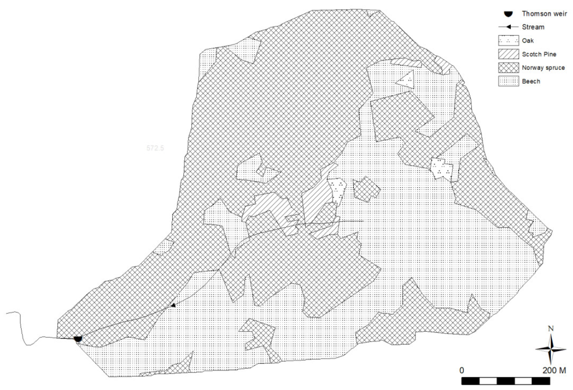
The experimental catchment is a forested headwater catchment with an area of 57 ha (Table 1). Its mean altitude reaches 520 m above sea level with eastern exposure and a mean catchment slope reaching 21%. The current forest stands are common production forests dominated by Norway spruce (Picea abies) (Figure 1). The soils are mainly inceptisols (Cambisols; Soil type according to Soil Survey Staff [31]).
2.2. Climatic Data
Near the catchment (within 1 km), a field climatic station (MeteoUNI, Amet, Velké Bílovice, Czech Republic) was installed in an open area of forest nursery grounds in 2016. The station has been in function with occasional failures (unexpected battery death, rain gauge breakage, etc.) and technological gaps (software upgrades, solar panel exchange, etc.) since its installation. Because the station does not include a heated rain gauge, it is unable to correctly read snow precipitation.
Given the technological limitations of the field climatic station, daily precipitation and temperature data were also obtained from the freely accessible climatic network European high-resolution gridded dataset (E-OBS), which is provided by the European Climate Assessment and Dataset project (ECA&D). The current version 21.0e was used. It offers data from 1950 to 2019 included in a grid of 0.1° latitude and longitude. In this part of the globe, this roughly corresponds to a rectangle with dimensions of 11.1 by 7.3 km. The center of the rectangle that was used in this case was located at 49.25° N; 16.65° E. The estimates of both precipitation and temperature values are created from a simulation of 100 spatial correlations (for more details, see [32]). Since the original construction of the E-OBS network [33], the number of included meteorological stations has increased over time, currently reaching 3700 temperature stations and 9000 precipitation stations. The highest density of stations is located in Scandinavia and Central Europe [32], which includes CR.
2.3. Hydrological Data
A Thomson weir for streamflow estimations is located in the discharge outlet of the catchment (Figure 1). The weir was installed in 2014, and the water level above its spillway has been continuously measured with winter and technological gaps or occasional failures since 2015. In 2015–2018, the water level was measured by a hydrostatic submersible pressure sensor (TSH22-3-1) connected to a datalogger (Hydro Logger H40D, both Fiedler AMS, České Budějovice, CR; [33].) The water-level values were automatically converted to streamflow by the datalogger every 15 min by a preset rating curve for the Thomson weir [34]. In 2019, the measuring system was upgraded to an ultrasound sensor US3200 with a combination HYDRO-LOGGER H2 datalogger (both Fiedler Automatic Monitoring Systems AMS, České Budějovice, CR), and roofing was installed over the watered area behind the spillway to mitigate some of the issues connected with objects (mostly branches and leaves) falling into the stream and causing measurement errors.
Similar to the field climatic station data and given the technological limitations (gaps in measurements caused by the stream surface freezing solid during the winter season), changes in technology (pressure vs. ultrasound sensor), and complications during storm flood events and low flow periods (more on this in the discussion), the streamflow data from the Thomson weir were utilized as a reference for streamflow simulation performed by the PERSiST hydrological model. The PERSiST model is a conceptual hydrological model with a daily time step that enables the simulation of water balance components even in small catchments. The model simulates the movement of precipitation water throughout the system by calculating interception, evapotranspiration, and infiltration in different hydrological horizons (called buckets) in the resulting streamflow [21]. The model is ongoing development, and version PERSiST_v1.6.1beta2 was used in this case.
2.4. The PERSiST Model Calibration Strategy
The driving data for the model were the daily series of precipitation and mean daily temperature obtained from the E-OBS database. The primary quantitative catchment properties (such as catchment area and stream length) were obtained from basic GIS analysis after catchment delineation. The qualitative parameters (landscape units and species composition) were obtained from the currently viable forest management plan.
The parametrization of the model was performed in several steps:
- 1.
- The realistic range of possible daily interception (1–3 mm/day) and mean daily evapotranspiration during the growing season (1–6 mm/day) was defined by a combination of values consistent with the recent literature, similar to the approach of Deutscher [35]. Measured local data [18] were obtained from close forested catchments in TFE, where historically detailed measuring campaigns took place [12,36,37]. The emphasis in this step was on realistically capturing the differences between evergreen coniferous (spruce) and deciduous (beech and larch) tree stands. Therefore, the catchment was divided into two specific landscape units representative of the areal distribution of deciduous and coniferous tree species, and the most important parameters were set up to incorporate the expected differences between the two stand types (Table 2). For example, the ratio of the maximum daily evapotranspiration of deciduous plants to conifers was kept between 20% and 30%, which should be expected in the region [12].
- 2.
- The model soil structure setup and the basic properties of individual hydrological soil horizons (soil buckets) were based on combining the results mentioned above from antecedent field measuring campaigns in similar nearby catchments and in situ measurements, including soil surveys [38], in a “bottom up” manner [39]. Soils in the catchment reach are 60–80 cm deep, and its maximum capillary capacity ranges from 29% to 35%. Three hydrologically distinct soil horizons (soil buckets) were selected from the soil stratigraphy to represent the fast-moving surface and shallow-depth runoff zone (upper runoff bucket), rooting zone (from which water is consumed for stand transpiration—Tanspiration zone bucket), and deep soil horizon responsible for sustaining base flow (deep runoff bucket). Retained water depth and maximum capacity of these buckets were estimated from the soil survey, similar to the protocol in Deutscher [35] using maximum capillary capacity and porosity respectively, to define realistic parameter range for these two user defined parameters. The soil parameters were not changed during the calibration process, with the exception of the initial water depth (which was changed to obtain the correct initial streamflow) and the time constant that we had no available relevant field measurements to base upon (this is where we used the temporal dynamics of the measured data as a reference for realistic streamflow behavior, most notably the quick one-day response to precipitation events).
- 3.
- Calibration was then performed manually against the periods of best available measured streamflow data (parts of 2019 after the ultrasound technology update), which is the most commonly used method [21] and own expertise. The periods with the best available measured streamflow data were also used to perform the model accuracy testing. However, since the measurements of streamflow in small forest streams are subject to a high amount of uncertainties [40,41], we used the measured dataset mostly as a reference. During periods with gaps in the measured data series, most importantly during winter periods, emphasis was placed on sustaining a reasonable minimum streamflow value such that the modeled streamflow would never be less than 0.2 L/s. This value was not observed in the stream since 2014, when monitoring of the catchment began. Ultimately, the overall performance of the model was reviewed by own expertise to determine whether the model reasonably simulated the expected temporal patterns in streamflow dynamics, such as quick reactions to precipitation events in small catchments [42], realistic recession curves in precipitation-free periods [33], and sustained reasonable streamflow during periods of low flow [12].
2.5. Temporal Trend Analysis
Complete temperature, precipitation (E-OBS), and streamflow (PERSiST) data series were obtained in the above-described manner for the experimental catchment in five consecutive years up to 2019. First, temporal trend analysis of these variables was performed for the conventional hydrological years in the European temperate zone, e.g., 1 November of the antecedent year to 31 October of the following year, resulting in a study period of 1 November 2014 to 31 October 2019 and five hydrological years. Second, given the seasonality of the temperate climate and the corresponding aspects of tree physiology and ecophysiology, the growing season (1 April to 31 October., 214 days) and the antecedent dormant season (1November of antecedent year to 31 March of the current year) were analyzed separately.
Simple linear trend analysis was performed on the total precipitation, total discharge, and mean daily temperature during the described periods (five hydrological years, five growing seasons, and five dormant seasons). For this purpose, specific discharge (L/m−2 or mm/m−2) was calculated from the mean daily streamflow values in each period. Linear trend analysis was also performed on the discharge coefficients in the same periods to enable a mediated estimation of precipitation usage in the catchment system. The interpretation of the observed temporal trends of these variables was performed by comparing the initial and ending values of the trend lines, which were obtained from the linear regression function (1).
Simple linear regression equation
which describes a line with slope b and y-intercept a.
y = a × x + b
3. Results
3.1. E-OBS and PERSiST Accuracy
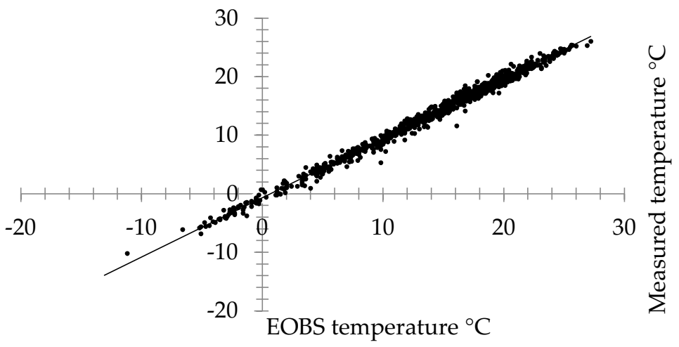
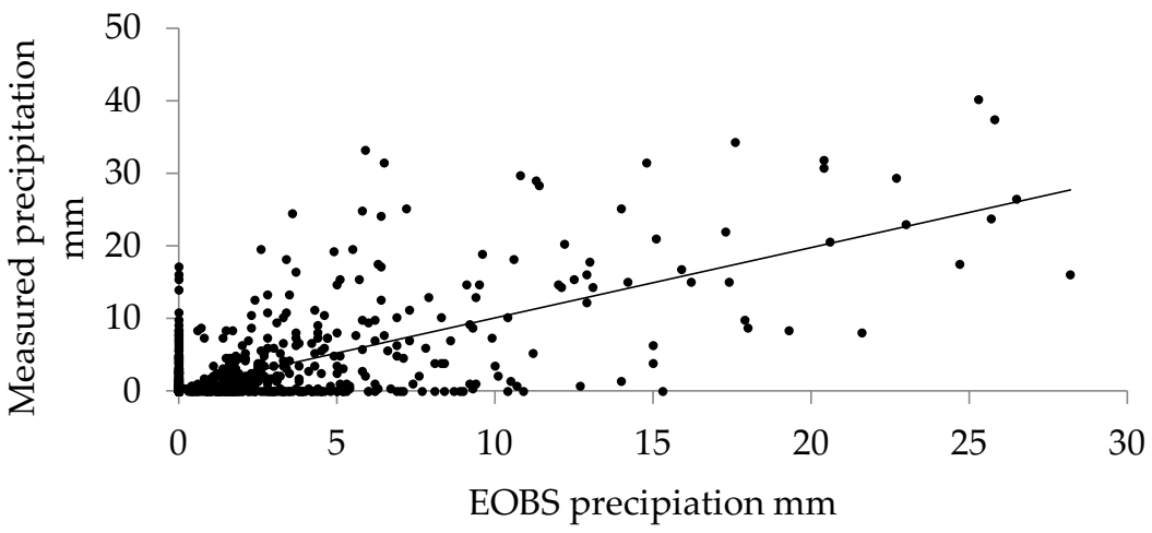
The accuracy of the E-OBS climatic data was verified against the data from the field climatic station (Figure 2 and Figure 3). A comparison between the measured and grid-ded data showed a high correlation (R2 0.99). Precipitation showed a lower correlation (R2 0.51). This lower correlation is probably mainly due to differences in the time regis-tration of precipitation events between the two sources (oftentimes it is one day; points close to the X and Y axes, Figure 2 and Figure 3). More importantly, the difference in the total sum of precipitation reaches only 18% (gridded data are underestimated), which indi-cates a higher overall correlation.
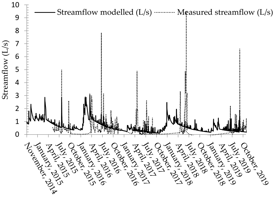
The overall performance of the PERSiST model reached R2 0.15, Nash–Sutcliffe 0.13 and RMSE 133 L per second (L/s) (Figure 4). Compared to occasional in situ manual water level measurements during weir maintenance (under standard water level conditions), it was better (R2 0.57; Nash–Sutcliffe 0.56; RMSE 60 L/s). The mean measured streamflow from all the available periods reached 0.69 L/s. The simulated streamflow for the same period reached 0.56 L/s. This result indicated an underestimation of modeled values by ca. 19%. This difference is likely caused by the driving precipitation data, which showed a similar underestimation (18%).
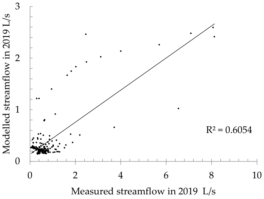
The model accuracy was tested in more detail against the best available measured data obtained by the updated ultrasound technology (since 2019) to minimize the effect of erroneous measurements. In this period, the model reached a correlation of R2 0.61 (Figure 5). The main differences could be observed during storm events, which indicated an overall underestimation of the simulated streamflow values. As mentioned before, the differences between measured and simulated streamflow might be caused by a slight shift in the registration of precipitation events in the driving climatic data (more in the discussion).
3.2. Characteristics of the Study Period
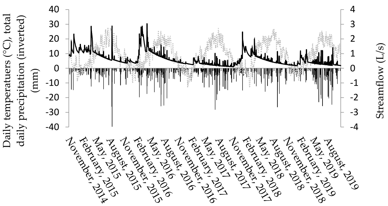
The mean daily simulated streamflow for the study period (1 November 2014 to 31 October 2019) reached 0.64 L/s, the mean daily temperature was 9.17 °C, and the mean annual precipitation was 510 mm (Table 3, Figure 6).
The long-term averages according to the 1980–2010 climatic standard for the South Moravian Region (obtained from the freely available database at Czech Hydrometeorological Institute) reach 559 mm of annual precipitation and 8.9 °C of mean daily temperature. All the hydrological years in the study period had lesser precipitation and higher temperature (Table 4).
Both precipitation and temperature increased during the period, while streamflow exhibited a decreasing trend (Table 4). When compared to the five-year standard, their observed temporal patterns can be characterized as follows: the interannual increase in temperature exceeded +9%, while the interannual decrease in streamflow reached almost –25%, and precipitation was rather stable throughout the period (the interannual change reached +0.02%).
3.3. The Trend Analysis in Hydrological Years
The trends of temperature, precipitation, and discharge over the five-year period were analyzed from the relative change that occurred during the period. The trend lines were constructed from the annual averages in the five hydrological years (Table 4). The relative change was calculated as the ratio of the initial value of the trend line (x = 1) to the difference between its initial (x = 1) and ending values (x = 5) (Table 5, Figure 7). The observed trends confirm the increase in temperature and precipitation as well as the decrease in discharge (streamflow) as mentioned above in the comparison of daily value trends to their five-year average (Table 3). This analysis of the relative change indicates that over the five-year period, discharge from the catchment decreased by more than −65%, even though precipitation increased by more than +11%.
3.4. The Trend Analysis of Seasonal Patterns
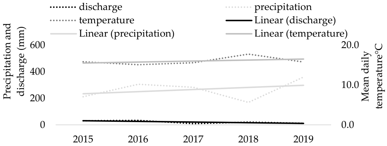
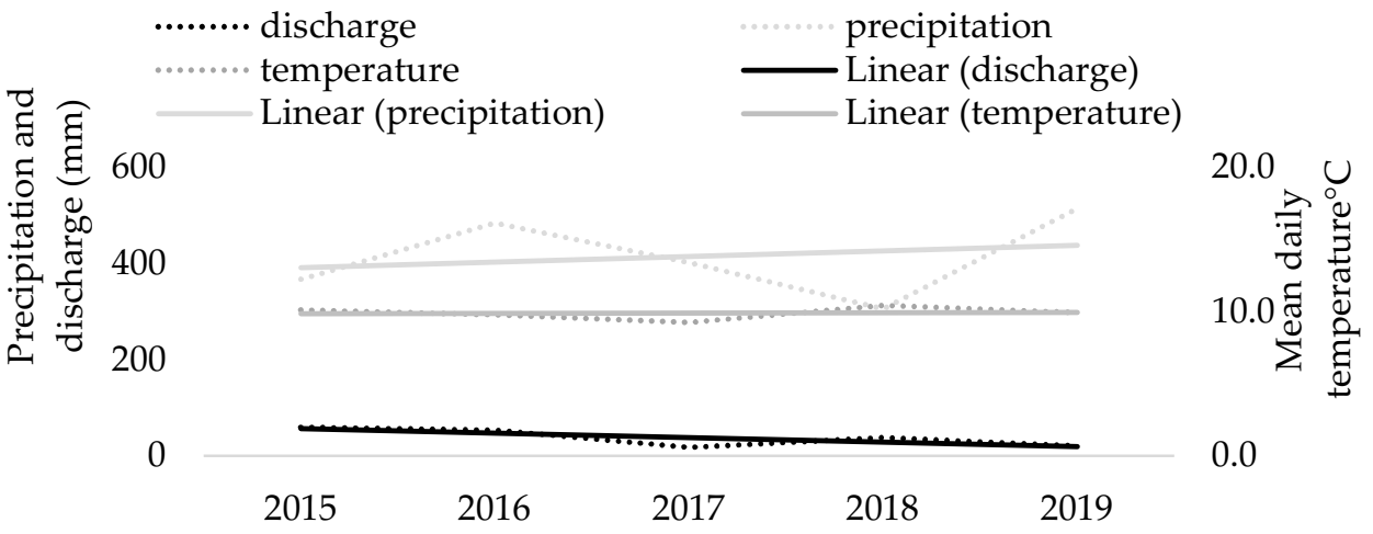
The decrease in discharge during the five-year study period seems very stable and high, reaching more than −65% in both growing and dormant seasons (Table 6, Figure 8 and Figure 9). The temperatures increased during the growing seasons (over +6%) but decreased throughout winter (−63%). The most important difference was found in the precipitation amounts occurring during the dormant season (a decrease of almost −11%) compared to the growing season, when an increase of over +27% occurred.
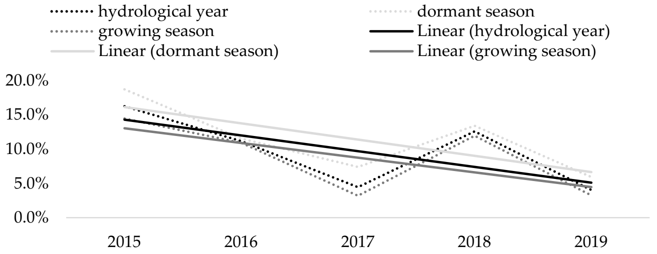
The runoff coefficient as a ratio of precipitation to runoff is used here as a simplified indicator of the inverse usage of water by the catchment. The lower the coefficient is, the higher the consumption of available water resources in the catchment is. During the growing season, the trends in the runoff coefficient seem to be equivalent to the trend in discharge (both decrease at similar rates over −65%; Table 7, Figure 10). This result indicates that the catchment’s water demands have increased by more than −65% during the growing season, which corresponds to the observed decrease in discharge even when precipitation increased (by +27%). This situation is different in the dormant season when the water usage does not increase as rapidly (−58%).
4. Discussion and Conclusions
Gridded climatic data from E-OBS [43] and the hydrological model PERSiST [21] were used to evaluate the temporal trends of streamflow during the last five years (2014–2019). The relevance of the gridded temperature and precipitation was verified by comparison to our own in situ measurements. The E-OBS dataset’s overall accuracy was deemed sufficient for this research purpose (model driving data). In contrast to the utilization of the E-OBS data in previous research by the authors in Hradec Králové city (1) [35], our study showed lower correlation in precipitation (R2 0.51 in this case as compared to 0.90 in (1)). This can be explained by the different comparison datasets used in the studies. In (1), data obtained from the Czech Hydrometeorological Institute (which represent interpolations from the closest meteorological stations) provide a similar model to E-OBS. In comparison, the present study uses our own in situ measurements performed near the catchment. Notably, the total sum over the five-year period was only 18% different. The main issue with the E-OBS dataset was not the amount of rainfall but the difference in the registration time of the precipitation events, which was sometimes shifted one day earlier or later. The sources of uncertainty of the local instrumental data as the main reasons for the lower correlations between precipitation values were explained in the methodology section (mainly the non-heated rainfall gauge, malfunction and battery death which occurred several times throughout the study period and can be considered a common issue for remote experimental sites in the forest). For the purpose of this research, we therefore opted for the E-OBS dataset that is not burdened by technological gaps and is free of erroneous measurements as opposed to the instrumental data [19], even though some microclimate specificity might have been lost due to the degree of generalization in the E-OBS dataset [20]. It should be noted that due to the gaps and high level of uncertainty in the instrumental data, no correction methods were applied to the dataset [44].
The hydrological model PERSiST seemed to be a good tool for the simulations in this research. Its ability to reproduce continuous streamflow patterns even on a very small catchment (57 ha) was crucial for filling the gaps and work around the uncertainties of the in situ estimations caused by erroneous measurements. Throughout the years of streamflow estimations at the Thomson weir, we encountered several issues with the technology connected to the nature of the in situ measurement design, some of which have been reported before from catchments with similar technology [45,46,47]. During stormflow, the increased flow magnitude may release pulses of wash load, bed material load as well as wood, that gets clogged in the spillway. This causes an unrealistic increase in observed streamflow. Therefore, the magnitude of the observed stormflow peaks comes with a high degree of uncertainty. During low flow, which in the Křtiny catchment corresponds approximately to 0.2–0.3 L/s, the water level of the spillway beam that is registered by the sensors is less than 4 cm. With such a small amount of water, single leaves can temporarily clog the spillway (this is very significant during leaf fall), which again causes some erroneous streamflow estimations and can disrupt the usually decreasing streamflow signal in the period [45]. To mitigate this issue in the future, roofing was placed above the weir basin (in 2019) to reach the effect of a trash screen [47]. Lastly, during frost periods, the hydraulics of the spillway change and the rating curve of the Thomson weir is no longer applicable [47]. That is why winter periods were excluded from the observed dataset. At the same time, the hydrostatic submersible pressure water level sensor that was used for most of the measured data (until 2019) is prone to exhibit decreasing accuracy during rapidly changing conditions (during storm events)—barometric pressure, air temperature, quick water level increase, changes in hydraulic pressure due to rapid sediment deposition, and so forth (Fiedler AMS, České Budějovice, CR).
All these sources of uncertainty happening on this small forest stream cause the need for a streamflow model in the first place. As mentioned in the methodology section, we used modeled data only for the trend analysis presented in the paper, and the measured streamflow was used as a guideline during the modelling exercise because common approaches of model accuracy (comparison to accurate measured data) [21] were not fully available in this case. Therefore, a “bottom up” unorthodox approach [39] based on good knowledge of the catchment (from in situ measuring campaigns) in combination with actual results published in the literature, used as references for setting realistic parameter range [35], was adopted.
Driven by the E-OBS gridded climatic data, it captured the temporal dynamics during standard water levels well, as reported in other works using the PERSiST model [35,48]. The model limitations in the present study’s case come mainly in the underestimation of observed streamflow peaks occurring after precipitation events, similar to the results discussed by Futter [48]. However, the main technological limitations of the water level registration technology used for the in situ streamflow estimations occurred at exactly the same time as discussed above. The underestimation of some of the flood events by the PERSiST model possibly could be explained by the streamflow measuring system not functioning properly and giving erroneous results, so-called “dissinformative observations” [49]. Detailed audit control of possible erroneous results and accuracy of the model was performed by comparing streamflow data measured by the updated technology since 2019, which used unsubmerged ultrasound sensors and should have been more stable and accurate under the conditions of stormflow, and the modeled data. In this specific period, the model reached accuracy of R2 0.60. Notably, the severity of the uncertainties in the instrumental dataset obtained throughout the experiment meant that it could not have been used as the only metric of model fit and therefore a subjective expert verification of expected streamflow behavior was performed and was deemed as similarly important (quick reactions to precipitation events [42], realistic recession curves in precipitation-free periods [33] and sustained low flow [12]). The obtained accuracy level indicates that the PERSiST calibration presented here as the result of the unorthodox approach can be deemed sufficient for the simulation of mean streamflow under standard water level conditions (occurring for most parts of the year).
This study’s modeling results, based on daily datasets (Table 3, Figure 6), indicate that the precipitation was stable, the temperature increased, and the streamflow/discharge decreased in the five-year period (1 November 2014 to 31 October 2019) in the studied catchment. This shows that with increasing temperature, the amount of water in the forest stream decreases.
Since transpiration is the main driving factor of the water balance of temperate forested catchments [9], the growing and the dormant seasons were analyzed separately as we assumed that the effect of vegetation would be better visible. For this reason, we used the hydrological year as the main evaluation period since it can be used as a defined water balance period. Since we worked with dormant seasons and growing seasons separately, we evaluated the trends from the individual hydrological years in this step. For the evaluation, the length and the time of the growing season were arbitrarily set the same for all the years (1 April to 31 October, 214 days). This period is slightly longer than the long-term averages of ca. 190 days typical for this region in the past [50] to incorporate ongoing climate changes [51]. A number of studies show that the length of the growing season has been increasing in the region by several weeks [7,52], most notably because of the earlier start of spring. However, our set definition of the growing season’s length does not allow us to account for possible interannual variability, which could be important [53].
In the context of the ongoing climate changes where drought effects have been reported in the region in the past 10 years [1,4,54], the combination of the simple linear trend and annual averages from studied hydrological years in the five-year period was used to depict the currently ongoing changes in the water balance of the catchment.
Our modeling indicates a significant increase in precipitation (+27.3%) during the growing season even though the discharge dramatically decreased (−65.6%, Table 6). This finding suggests that the increasing transpiration demands driven by increasing temperatures and their effects on streamflow are unexpectedly disproportional since temperature exhibited an increasing trend of +6.5% while discharge exhibited a decreasing trend of −65.6%. Similar discharge patterns were observed during the dormant season. In this case, the driving force was probably not temperature, which exhibited only a slight increasing trend (+1.2%), but rather the decreasing precipitation (−11%). These observed patterns of lower winter precipitation seem to be more common in the region and might become the new standard [55].
These results obtained by the simple linear regression are in accord with previously published studies from the region. Blöschl et al. [56] demonstrated that between 1960 and 2010, decreasing winter snow precipitation led to a decreasing flood trend in Eastern Europe and increasing autumn and winter precipitation led to an increasing flood trend in Northwestern Europe. CR lies in the middle of the two regions and seemed to be affected by both of these signals in the five-year study period since both an increase in temperature and an increase in precipitation were found. Our modelled decrease in discharge coefficient (more than −65% in 2015–2019, Table 7) could be representative of the continuation of the decreasing flood trend identified by Blöschl et al. [56] in 2000–2010 in the CR. In a recent modelling study from the CR, Řehoř et al. [57] reported that a significant occurrence of soil drought has been found in the Moravian parts of the CR both summer and winter periods.
The increasing temperatures mean that in winter, a higher proportion of the precipitation falls in a liquid state and ground does not freeze solid, leading to a bigger proportion of water infiltrating the soil [58], and also leading to higher winter evapotranspiration caused by coniferous stands not being fully dormant during mild winters [59]. This, in combination with decreasing winter precipitation (−11%; Table 6), can be the reason why the catchment’s water use in our simulation during the dormant season was only reduced by 7% (Table 7) in comparison to the growing season. At the same time, the earlier start of the growing season leads to the occurrence of severe soil water depletion during summer [57], which means that not enough water is available for sufficient ground water recharge, as indicated by the runoff ratio presented in Table 7. Lack of winter groundwater recharge not only poses a risk to water availability but also might cause water stress to forest stands in the spring when they are in increased need of water to support leaf out. As a result, the forests in the region have suffered from lack of water quite severely during the last years [60].
The decreasing streamflow can be connected to the effects increasing temperature has on vegetation. Increasing temperatures prolong the growing season [7] by its earlier start [6]. The increasing transpiration demands increase the water consumption by the stands and limit the water use efficiency of the catchment [37], as shown by the decreasing trends in the runoff ratios (Table 7). However, there also seems to be some reverse effects associated with increasing concentrations of CO2 in the atmosphere, which can limit transpiration and stomata conductivity [61], as well as the water depletion in the summer period [57], which can limit transpiration as well. Our simulations identified a decreasing trend in streamflow of 65% over the course of the five years. This corresponds to a 13% reduction in streamflow per year.
Our modeling results show that a trend of decreasing water amounts in the forest stream of the experimental catchment Křtiny (indicated by streamflow and discharge results in this study) occurred in the five-year study period (1 November 2014 to 31 October 2019) even despite increasing precipitation. As discussed above, the decrease is most likely caused by increasing temperature and its subsequent second–order effects. It can indicate two important aspects that occurred in the catchment during these five years:
- A decreasing discharge (−65%), despite an increase in precipitation during the growing season (+27%), indicates that increasing temperature causes an increase in water demand in the catchment that cannot be offset even by the increase in precipitation.
- A lack of winter precipitation related to increasingly warmer dormant seasons can be associated with less snow cover and higher evapotranspiration, which causes even further water depletion.
An unexpected disproportion was found in the increasing temperature to decreasing discharge during the growing season, which can be simplified to an increasing trend in the mean daily temperature of +1% per season, effectively causing a decreasing trend in the discharge of −10% per season, regardless of the increasing precipitation during the period.
This paper presents a unique approach to work around some of the common uncertainties in local field data by using replacement climatic data and expert knowledge of the catchment. Importantly, it also showcases the importance of understanding the user defined model parameters to be able to obtain the right answer for the right reasons [49]. The modeling results obtained this way are in accord with more robust modelling campaigns of other authors from the region. This suggests that a similar approach could have its place in the modelling practice but at the same time should be limited for simulations of standard water level conditions where it offers best results.
Author Contributions
Conceptualization, P.K.; methodology, P.K. and J.D.; software, J.D. and O.H.; validation, P.K., J.D. and O.H.; formal analysis, O.H.; investigation, J.D.; resources, J.D.; data curation, J.D. and O.H.; writing—original draft preparation, P.K.; writing—review and editing, J.D. and O.H..; visualization, O.H.; supervision, P.K.; funding acquisition, J.D. All authors have read and agreed to the published version of the manuscript.
Funding
The authors were supported by the project “Strengthening and development of inventive activities at the Faculty of Forestry and Wood technology Mendel University in Brno by creating post-doc positions–project 7.1 of Institutional plan of Mendel University 2019−2020.”
Institutional Review Board Statement
Not applicable for studies not involving humans.
Informed Consent Statement
Not applicable for studies not involving humans.
Data Availability Statement
Data is available from the authors on request.
Acknowledgments
We acknowledge the E-OBS dataset from the EU-FP6 project UERRA (http://www.uerra.eu, accessed on 12 February 2021) and the data providers in the ECA&D project (https://www.ecad.eu, accessed on 12 February 2021). We acknowledge the Internal Grant Agency (IGA) of the Faculty of Forestry and Wood Technology (FFWT) of Mendel University in Brno that supported the authors as part of the project LDF_TP_2019002.
Conflicts of Interest
The authors declare no conflict of interest.
References
- Trnka, M.; Balek, J.; Zahradníček, P.; Eitzinger, J.; Formayer, H.; Turňa, M.; Nejedlík, P.; Semerádová, D.; Hlavinka, P.; Brázdil, R. Drought trends over part of Central Europe between 1961 and 2014. Clim. Res. 2016, 70, 143–160. [Google Scholar] [CrossRef] [Green Version]
- Donnelly, C.; Greuell, W.; Andersson, J.; Gerten, D.; Pisacane, G.; Roudier, P.; Ludwig, F. Impacts of climate change on European hydrology at 1.5, 2 and 3 degrees mean global warming above preindustrial level. Clim. Change 2017, 143, 13–26. [Google Scholar] [CrossRef] [Green Version]
- Neary, D.G.; Ice, G.G.; Jackson, C.R. Linkages between forest soils and water quality and quantity. For. Eco. Man. 2009, 258, 2269–2281. [Google Scholar] [CrossRef]
- Moravec, V.; Markonis, Y.; Rakovec, O.; Kumar, R.; Hanel, M. A 250-year european drought inventory derived from ensemble hydrologic modeling. Geoph. Res. Lett. 2019, 46, 5909–5917. [Google Scholar] [CrossRef]
- Spinoni, J.; Vogt, J.V.; Naumann, G.; Barbosa, P.; Dosio, A. Will drought events become more frequent and severe in Europe? Int. J. Climatol. 2018, 38, 1718–1736. [Google Scholar] [CrossRef] [Green Version]
- Menzel, A.; Yuan, Y.; Matiu, M.; Sparks, T.; Scheifinger, H.; Gehrig, R.; Estrella, N. Climate change fingerprints in recent european plant phenology. Glob. Chang. Biol. 2020, 26, 2599–2612. [Google Scholar] [CrossRef] [Green Version]
- Lian, X.; Piao, S.; Li, L.Z.X.; Li, Y.; Huntingford, C.; Ciais, P.; Cescatti, A.; Janssens, I.A.; Peñuelas, J.; Buermann, W.; et al. Summer soil drying exacerbated by earlier spring greening of northern vegetation. Sci. Adv. 2020, 6. [Google Scholar] [CrossRef] [Green Version]
- Grelle, A.; Lundberg, A.; Lindroth, A.; Moren, A.; Cienciala, E. Evaporation components of a boreal forest: Variations during the growing season. J. Hydrol. 1997, 197, 70–87. [Google Scholar] [CrossRef]
- Schlesinger, W.H.; Jasechko, S. Transpiration in the global water cycle. Agric. For. Meteorol. 2014, 189–190, 117–155. [Google Scholar] [CrossRef]
- Mátyás, C.; Sun, G. Forests in a water limited world under climate change. Env. Res. Lett. 2014, 9. [Google Scholar] [CrossRef] [Green Version]
- Kovář, P.; Bačinová, H. Impact of evapotranspiration on diurnal discharge fluctuation determined by the Fourier series model in dry periods. Soil Water Res. 2015, 10, 210–217. [Google Scholar] [CrossRef] [Green Version]
- Deutscher, J.; Kupec, P.; Dundek, P.; Holík, L.; Machala, M.; Urban, J. Diurnal dynamics of streamflow in an upland forested micro-watershed during short precipitation-free periods is altered by tree sap flow. Hydrol. Process. 2016, 30, 2042–2049. [Google Scholar] [CrossRef]
- Černohous, V.; Švihla, V.; Šach, F. Manifestation of drought in spruce pole-stage stand in summer 2015. Zpravy Lesnickeho Vyzkumu 2018, 63, 10–19. [Google Scholar]
- Brown, A.E.; Zhang, L.; McMahon, T.A.; Western, A.W.; Vertessy, R.A. A review of paired catchment studies for determining changes in water yield resulting from alterations in vegetation. J. Hydrol. 2005, 310, 28–61. [Google Scholar] [CrossRef]
- Beven, K. A manifesto for the equifinality thesis. J. Hydrol. 2006, 320, 18–36. [Google Scholar] [CrossRef] [Green Version]
- Kampf, S.K.; Burges, S.J. A framework for classifying and comparing distributed hillslope and catchment hydrologic models. Water Resour. Res. 2007, 43. [Google Scholar] [CrossRef] [Green Version]
- Hrachowitz, M.; Savenije, H.H.G.; Blöschl, G.; McDonnell, J.J.; Sivapalan, M.; Pomeroy, J.W.; Arheimer, B.; Blume, T.; Clark, M.P.; Ehret, U. A decade of Predictions in Ungauged Basins (PUB) A review. Hydrol. Sci. J. 2013, 58, 1198–1255. [Google Scholar] [CrossRef]
- Seibert, J.; McDonnell, J.J. On the dialog between experimentalist and modeler in catchment hydrology: Use of soft data for multicriteria model calibration. Water Resour. Res. 2002, 38, 23-1–23-14. [Google Scholar] [CrossRef]
- Ledesma, J.L.J.; Futter, M.N. Gridded climate data products are an alternative to instrumental measurements as inputs to rainfall–runoff models. Hydrol. Process. 2017, 31, 1–11. [Google Scholar] [CrossRef] [Green Version]
- Renard, B.; Kavetski, D.; Kuczera, G.; Thyer, M.; Franks, S.W. Understanding predictive uncertainty in hydrologic modeling: The challenge of identifying input and structural errors. Water Resour. Res. 2010, 46. [Google Scholar] [CrossRef]
- Futter, M.N.; Erlandsson, M.A.; Butterfield, D.; Whitehead, P.G.; Oni, S.K.; Wade, A.J. PERSiST: A flexible rainfall-runoff modelling toolkit for use with the INCA family of models. Hydrol. Earth Syst. Sci. 2014, 18, 855–873. [Google Scholar] [CrossRef] [Green Version]
- Šimůnek, J.; Van Genuchten, M.T.; Šejna, M. Recent developments and applications of the HYDRUS computer software packages. Vadose Zone J. 2016, 15. [Google Scholar] [CrossRef] [Green Version]
- Gassman, P.W.; Reyes, M.R.; Green, C.H.; Arnold, J.G. The soil and water assessment tool: Historical development, applications, and future research directions. Trans. ASABE 2007, 50, 1211–1250. [Google Scholar] [CrossRef] [Green Version]
- Douglas-Mankin, K.R.; Srinivasan, R.; Arnold, J.G. Soil and Water Assessment Tool (SWAT) model: Current developments and applications. Trans. ASABE 2010, 53, 1423–1431. [Google Scholar] [CrossRef]
- Lindström, G.; Pers, C.; Rosberg, J.; Strömqvist, J.; Arheimer, B. Development and testing of the HYPE (Hydrological Predictions for the Environment) water quality model for different spatial scales. Hydrol. Res. 2010, 41, 295–319. [Google Scholar] [CrossRef]
- Guo, A.; Huang, Q.; Wang, Y.; Li, Y. Detection of variations in precipitation-runoff relationship based on Archimedean Copula. J. Hydroelectr. Eng. 2015, 34, 7–13. [Google Scholar]
- De Luca, D.L.; Biondi, D. Bivariate Return Period for Design Hyetograph and Relationship with T-Year Design Flood Peak. Water 2017, 9, 673. [Google Scholar] [CrossRef] [Green Version]
- Yang, Y.; Weng, B.; Man, Z.; Yu, Z.; Zhao, J. Analyzing the contributions of climate change and human activities on runoff in the Northeast Tibet Plateau. J. Hydrol. Reg. Stud. 2020, 27, 100639. [Google Scholar] [CrossRef]
- Demek, J. Obecná Geomorfologie; Academia: Prague, Czech Republic, 1987; p. 476. [Google Scholar]
- Bajer, A. Krajina a Geodiverzita: Neživá Příroda jako Základ Krajinných a Kulturních Hodnot; Mendelova Univerzita v Brně: Brno, Czech Republic, 2015. [Google Scholar]
- Soil Survey Staff. Soil Taxonomy: A Basic System of Soil Classification for Making and Interpreting soil Surveys, 2nd ed.; Handbook 436, US; Natural Resources Conservation Service, U.S. Department of Agriculture: Washington, DC, USA, 1999.
- Cornes, R.; van der Schrier, G.; van den Besselaar, E.J.M.; Jones, P.D. An Ensemble Version of the E-OBS Temperature and Precipitation Datasets. J. Geophys. Res. Atmos. 2008, 123, 9391–9409. [Google Scholar] [CrossRef] [Green Version]
- Haylock, M.R.; Hofstra, N.; Tank, A.; Klok, E.J.; Jones, P.D.; New, M. A European daily high-resolution gridded data set of surface temperature and precipitation for 1950–2006. J. Geophys. Res. Atmos. 2008, 113. [Google Scholar] [CrossRef] [Green Version]
- Kupec, P.; Deutscher, J. Streamflow diurnal dynamics of upland microwatersheds during precipitation-free periods. Zpravy Lesnickeho Vyzkumu 2016, 61, 190–196. [Google Scholar]
- Deutscher, J.; Kupec, P. Monitoring and validating the temporal dynamics of interday streamflow from two upland head micro-watersheds with different vegetative conditions during dry periods of the growing season in the bohemian massif, Czech Republic. Environ. Monit. Assess. 2014, 186, 3837–3846. [Google Scholar] [CrossRef]
- Deutscher, J.; Kupec, P.; Kučera, A.; Urban, J.; Ledesma, J.L.J.; Futter, M.N. Ecohydrological consequences of tree removal in an urban park evaluated using open data, free software and a minimalist measuring campaign. Sci. Total Environ. 2019, 655, 1495–1504. [Google Scholar] [CrossRef] [PubMed]
- Deutscher, J.; Holík, L.; Kupec, P.; Marková, I.; Barašová, J.; Divín, J.; Holata, F.; Nezval, O.; Rosíková, J.; Školoud, L.; et al. Estimation of Basic Water-Balance Parameters of the Útěchov Forested Microwatershed. In Proceedings of the SilvaNet–WoodNet 2016: Proceedings Abstracts of Student Scientific Conference, Brno, Czech Republic, 14 November 2016; Martinek, P., Prouza, M., Čermáková, V., Rozsypálek, J., Eds.; Mendelova Univerzita v Brně: Brno, Czech Republic, 2016; pp. 27–28. [Google Scholar]
- Kupec, P.; Školoud., L.; Deutscher, J. Tree species composition influences differences in water use efficiency of upland forested microwatersheds. Eur. J. For. Res. 2018, 137, 477–487. [Google Scholar]
- Valtera, M.; Juřička, D.; Pálková, L.; Chytilová, M.; Patočka, Z.; Raschmann, G.; Hemr, O.; Matoušková, M.; Deutscher, J.; Urban, J. Effects of the Pit-Mound Microrelief in Forest Soils on Soil Moisture and Tree Growth in Spruce: Preliminary Results. In Proceedings of the SilvaNet–WoodNet 2019: Proceedings Abstracts of Student Scientific Conference, Brno, Czech Republic, 29 November 2019; Hemr, O., Kupská, M., Sedláčková, K., Eds.; Mendelova Univerzita v Brně: Brno, Czech Republic, 2019; pp. 67–68. [Google Scholar]
- Konrad, C.P.; Booth, D.B. Hydrologic Trends Associated With Urban Development for Selected Streams in Western Washington. In Water-Resources Investigations Report; U.S. Geological Survey: Reston, VI, USA, 2002; 40p. [Google Scholar]
- Mcmillan, H.; Krueger, T.; Freer, J. Benchmarking observational uncertainties for hydrology: Rainfall, river discharge and water quality. Hydrol. Process. 2012, 26, 4078–4111. [Google Scholar] [CrossRef]
- Ledvinka, O.; Lamacova, A. Detection of field significant long-term monotonic trends in spring yields. Stoch. Environ. Res. Risk Assess. 2015, 29, 1463–1484. [Google Scholar] [CrossRef]
- Ribolzi, O.; Andrieux, P.; Valles, V.; Bouzigues, R.; Bariac, T.; Voltz, M. Contribution of groundwater and overland flows to storm flow generation in a cultivated Mediterranean catchment. Quantification by natural chemical tracing. J. Hydrol. 2010, 233, 241–257. [Google Scholar] [CrossRef]
- Smitha, P.S.; Narasimhan, B.; Sudheer, K.P.; Annamalai, H. An improved bias correction method of daily rainfall data using a sliding window technique for climate change impact assessment. J. Hydrol. 2018, 556, 100–118. [Google Scholar] [CrossRef]
- Doležal, F.; Kulhavý, Z.; Kvítek, T.; Soukup, M.; Čmelík, M.; Fučík, P.; Tippl, M. Hydrologický výzkum v malých zemědělských povodích. J.H.H. 2006, 54, 217–229. [Google Scholar]
- Gomi, T.; Dan Moore, R.; Hassan, M.A. Suspended sediment dynamics in small forest streams of the Pacific Northwest 1. JAWRA 2005, 41, 877–898. [Google Scholar] [CrossRef]
- Reinhart, K.G.; Pierce, R.S. Stream-Gaging Stations for Research on Small Watersheds; (No. 268); US Government Publishing Office: Washington, DC, USA, 1964.
- Futter, M.N.; Whitehead, P.G.; Sarkar, S.; Rodda, H.; Crossman, J. Rainfall runoff modelling of the Upper Ganga and Brahmaputra basins using PERSiST. Env. Sci. Process. Impacts 2015, 17, 1070–1081. [Google Scholar] [CrossRef] [Green Version]
- Beven, K.; Westerberg, I. On red herrings and real herrings: Disinformation and information in hydrological inference. Hydrol. Process. 2011, 25, 1676–1680. [Google Scholar] [CrossRef]
- Menzel, A.; Fabian, P. Growing season extended in europe. Nature 1999, 397, 659. [Google Scholar] [CrossRef]
- Jeong, S.; Ho, C.; Gim, H.; Brown, M.E. Phenology shifts at start vs. end of growing season in temperate vegetation over the northern hemisphere for the period 1982-2008. Glob. Chan. Biol. 2011, 17, 2385–2399. [Google Scholar] [CrossRef]
- Linderholm, H.W. Growing season changes in the last century. Agric. For. Meteorol. 2006, 137, 1–14. [Google Scholar] [CrossRef]
- Chmielewski, F.M.; Roetzer, T. Response of tree phenology to climate change across Europe. Agric. For. Meteorol. 2001, 108, 101–112. [Google Scholar] [CrossRef]
- Lamačová, A.; Hruška, J.; Krám, P.; Stuchlík, E.; Farda, A.; Chuman, T.; Fottová, D. Runoff trends analysis and future projections of hydrological patterns in small forested catchments. Soil. Water Res. 2014, 9, 169–181. [Google Scholar] [CrossRef] [Green Version]
- Trenberth, K.E.; Dai, A.; Rasmussen, R.M.; Parsons, D.B. The changing character of precipitation. BAMS 2003, 84, 1205–1217. [Google Scholar] [CrossRef]
- Blöschl, G.; Hall, J.; Viglione, A.; Perdigão, R.A.; Parajka, J.; Merz, B.; Živković, N. Changing climate both increases and decreases European river floods. Nature 2019, 573, 108–111. [Google Scholar] [CrossRef]
- Řehoř, J.; Brázdil, R.; Trnka, M.; Řezníčková, L.; Balek, J.; Možný, M. Regional effects of synoptic situations on soil drought in the Czech Republic. Theor. Appl. Climatol. 2020, 141, 1383–1400. [Google Scholar] [CrossRef]
- Sevanto, S.; Suni, T.; Pumpanen, J.; Grönholm, T.; Kolari, P.; Nikinmaa, E.; Hari, P.; Vesala, T. Wintertime photosynthesis and water uptake in a boreal forest. Tree Physiol. 2006, 26, 749–757. [Google Scholar] [CrossRef] [PubMed] [Green Version]
- Clausnitzer, F.; Köstner, B.; Schwärzel, K.; Bernhofer, C. Relationships between canopy transpiration, atmospheric conditions and soil water availability-analyses of long-term sap-flow measurements in an old norway spruce forest at the ore Mountains/Germany. Agric. For. Meteorol. 2011, 151, 1023–1034. [Google Scholar] [CrossRef]
- Toth, D.; Maitah, M.; Maitah, K.; Jarolínová, V. The Impacts of Calamity Logging on the Development of Spruce Wood Prices in Czech Forestry. Forests 2020, 11, 283. [Google Scholar] [CrossRef] [Green Version]
- Hasper, T.B.; Wallin, G.; Lamba, S.; Hall, M.; Jaramillo, F.; Laudon, H.; Linder, S.; Medhurst, J.L.; Rantfors, M.; Sigurdsson, B. Water use by Swedish boreal forests in a changing climate. Funct. Ecol. 2016, 30, 690–699. [Google Scholar] [CrossRef] [Green Version]
Figure 1.
Vegetation map of the study catchment.

Figure 2.
Gridded (European high-resolution gridded dataset—E-OBS) vs. measured (field climatic station) temperatures.
Figure 2.
Gridded (European high-resolution gridded dataset—E-OBS) vs. measured (field climatic station) temperatures.

Figure 3.
Gridded (E-OBS) vs. measured (field climatic station) precipitation.

Figure 4.
Modeled vs. measured streamflow (note that the gaps in between the observed data are automatically connected by straight lines).
Figure 4.
Modeled vs. measured streamflow (note that the gaps in between the observed data are automatically connected by straight lines).

Figure 5.
Modeled vs. measured streamflow in 2019.

Figure 6.
Mean daily values for temperature (grey line), precipitation (inverted line) and streamflow (doted black line) in the study period 1 November 2014 to 31 October 2019 in the experimental catchment Křtiny. Temperature and precipitation were obtained from the E-OBS dataset. Streamflow values were modelled in PERSiST.

Figure 7.
Hydrological years—discharge, precipitation, and mean temperature. Dotted are the annual averages for given years.
Figure 7.
Hydrological years—discharge, precipitation, and mean temperature. Dotted are the annual averages for given years.

Figure 8.
Growing seasons—discharge, precipitation and mean temperature. Dotted are the annual averages for given years.
Figure 8.
Growing seasons—discharge, precipitation and mean temperature. Dotted are the annual averages for given years.

Figure 9.
Dormant seasons—discharge, precipitation and mean temperature. Dotted are the annual averages for given years.
Figure 9.
Dormant seasons—discharge, precipitation and mean temperature. Dotted are the annual averages for given years.

Figure 10.
Annual and seasonal runoff coefficients (%). Dotted are the annual averages for given years.
Figure 10.
Annual and seasonal runoff coefficients (%). Dotted are the annual averages for given years.


Table 1.
Characteristics of the experimental catchment Křtiny.
| Area (ha) | 57 |
|---|---|
| Main stream length (m) | 940 |
| Max. elevation a.s.l. (m) | 563 |
| Min. elevation a.s.l. (m) | 456 |
| Mean elevation a.s.l. (m) | 521 |
| Exposure | Eastern |
| Mean catchment slope (%) | 21 |
| Ratio of coniferous (of which spruce) | 56 (43%) |
| Ratio of deciduous (including larix) | 44% |
Table 2.
Most relevant Precipitation, Evapotranspiration and Runoff Simulator for Solute Transport (PERSiST) parameters regarding vegetation properties.
Table 2.
Most relevant Precipitation, Evapotranspiration and Runoff Simulator for Solute Transport (PERSiST) parameters regarding vegetation properties.
| PERSiST Parameter | Deciduous | Coniferous |
|---|---|---|
| Canopy interception (mm/day) | 1.5 | 2 |
| Growing degree threshold (°C) | 7 | 1.5 |
| Solar radiation scaling factor | 70 | 120 |
Table 3.
The simple linear regression parameters for precipitation, temperature, and discharge for the whole study period 1 November 2014 to 31 October 2019 in the experimental catchment Křtiny calculated from daily values. The annual trend is calculated as a times the number of days in a year. The five-year standard is the mean annual value from the 5 years. The interannual change is calculated as a ratio of the annual change to the five-year standard.
| a | b | Annual Trend | Five-Year Standard | The Interannual Change | |
|---|---|---|---|---|---|
| Temperature | 0.0023 | 7.0684 | 0.84 | 9.17 | 9.17% |
| Precipitation | 0.0003 | −12.54 | 0.12 | 510.52 | 0.02% |
| Discharge | −0.0004 | 1.04 | −0.16 | 0.64 | −24.68% |
Table 4.
Characteristics of hydrological years. The discharge coefficient is calculated as the ratio of annual discharge to annual precipitation.
Table 4.
Characteristics of hydrological years. The discharge coefficient is calculated as the ratio of annual discharge to annual precipitation.
| Hydrological Year | Temperature °C | Precipitation mm | Discharge mm | Discharge Coefficient |
|---|---|---|---|---|
| 2015 | 10.1 | 366.7 | 59.6 | 16% |
| 2016 | 9.8 | 484.1 | 54.0 | 11% |
| 2017 | 9.2 | 401.7 | 17.8 | 4% |
| 2018 | 10.4 | 305.6 | 38.5 | 13% |
| 2019 | 9.9 | 514.1 | 20.8 | 4% |
Table 5.
The simple linear regression parameters for precipitation, temperature, and discharge in the study period 1 November 2014 to 31 December 2019 in the experimental catchment Křtiny calculated from annual averages in the five hydrological years.
Table 5.
The simple linear regression parameters for precipitation, temperature, and discharge in the study period 1 November 2014 to 31 December 2019 in the experimental catchment Křtiny calculated from annual averages in the five hydrological years.
| a | b | Initial Value of y | Ending Value of y | Change of y in the Period | Relative Change % | |
|---|---|---|---|---|---|---|
| Temperature | 0.03 | 9.81 | 9.83864 | 9.64 | 0.11776 | 1.20% |
| Precipitation | 11.63 | 379.55 | 391.18 | 437.7 | 46.52 | 11.89% |
| Discharge | −9.31 | 66.11 | 56.79391 | 19.54019 | −37.25372 | −65.59% |
Table 6.
The simple linear regression parameters for precipitation, temperature, and discharge in the growing (214 days) and dormant (151 days) seasons in the study period 1 November 2014 to 31 October 2019 in the experimental catchment Křtiny.
Table 6.
The simple linear regression parameters for precipitation, temperature, and discharge in the growing (214 days) and dormant (151 days) seasons in the study period 1 November 2014 to 31 October 2019 in the experimental catchment Křtiny.
| a | b | Initial Value of y | Ending Value of y | Change of y in the Period | Relative Change % | ||
|---|---|---|---|---|---|---|---|
| Growing season | Temperature | 0,25 | 15,25 | 15,50 | 16,51 | 1,01 | 6.52% |
| Precipitation | 15,94 | 217,94 | 233,88 | 297,64 | 63,76 | 27.26% | |
| Discharge | −5,12 | 36,31 | 31,20 | 10,72 | −20,48 | −65.58% | |
| Dormant season | Temperature | −0,29 | 2,10 | 1,81 | 0,66 | −1,15 | 1.20% |
| Precipitation | −4,31 | 161,61 | 157,30 | 140,06 | −17,24 | −10.96% | |
| Discharge | −4,19 | 29,77 | 25,57 | 8,79 | −16,78 | −65.61% |
Table 7.
The simple linear regression parameters for the runoff coefficient (precipitation/runoff ratio) in the hydrological year and growing (214 days) and dormant (151 days) seasons in the study period 1 November 2014 to 31 October 2019 in the experimental catchment Křtiny.
Table 7.
The simple linear regression parameters for the runoff coefficient (precipitation/runoff ratio) in the hydrological year and growing (214 days) and dormant (151 days) seasons in the study period 1 November 2014 to 31 October 2019 in the experimental catchment Křtiny.
| Runoff Coefficient | a | b | Initial Value of y | Ending Value of y | Change of y in the Period | Relative Change % |
|---|---|---|---|---|---|---|
| Hydrological year | −0.02 | 0.17 | 0.14 | 0.05 | −0.09 | −64.34% |
| Growing season | −0.02 | 0.15 | 0.13 | 0.04 | −0.09 | −65.64% |
| Dormant season | −0.02 | 0.19 | 0.16 | 0.07 | −0.09 | −58.70% |
Publisher’s Note: MDPI stays neutral with regard to jurisdictional claims in published maps and institutional affiliations. |
© 2021 by the authors. Licensee MDPI, Basel, Switzerland. This article is an open access article distributed under the terms and conditions of the Creative Commons Attribution (CC BY) license (https://creativecommons.org/licenses/by/4.0/).
Share and Cite
MDPI and ACS Style
Deutscher, J.; Hemr, O.; Kupec, P. A Unique Approach on How to Work Around the Common Uncertainties of Local Field Data in the PERSiST Hydrological Model. Water 2021, 13, 1143. https://doi.org/10.3390/w13091143
AMA Style
Deutscher J, Hemr O, Kupec P. A Unique Approach on How to Work Around the Common Uncertainties of Local Field Data in the PERSiST Hydrological Model. Water. 2021; 13(9):1143. https://doi.org/10.3390/w13091143
Chicago/Turabian StyleDeutscher, Jan, Ondřej Hemr, and Petr Kupec. 2021. "A Unique Approach on How to Work Around the Common Uncertainties of Local Field Data in the PERSiST Hydrological Model" Water 13, no. 9: 1143. https://doi.org/10.3390/w13091143
Note that from the first issue of 2016, this journal uses article numbers instead of page numbers. See further details here.