Prioritizing Design Parameters for Stepped Chutes and Shear Stress Distribution

Abstract

Stepped chutes offer high efficiency in decreasing flow velocity due to roughness; however, negative impacts may still be experienced by the receiving water body into downstream. These effects might be mitigated if geometric and hydraulic parameters governing the structure are well addressed. Herein, five influential parameters were developed, i.e., longitudinal slope S (S = tan θ), discharge (Q), pool height above steps (h_p), chute width (W), and chute height (H), employing a three dimensional (3D) numerical model. Through 600 simulations, two regression models were developed for predicting depth-averaged velocity at the last step V_d (m/s) and critical length L_c (cm) at the downstream where the maximum velocity occurs, using response surface methodology (RSM) based on the mixed-level full factorial design. The prediction data obtained by developed regression models were agreeable with actual data with coefficient determination (R²) of about 0.95, highlighting the accuracy and ability of the models for the prediction of V_d and L_c. Additionally, the analysis of variance (ANOVA) was used to prioritize the impact of the studied parameters on V_d and L_c. Results highlighted that among geometric parameters, W and $S$ had a significant influence on V_d and L_c; however, the impact of W was more pronounced. Using a regression model for L_c, a cross section was obtained, and the shear stress distribution of the downstream was compared with that of the last step and sidewalls. The shear stress patterns showed that the maximum value shifted from the side walls to the downstream between the lower and higher slopes. Further, the longitudinal distribution of shear stress at the downstream revealed that geometric and hydraulic characteristics played a negligible role in the changing pattern of shear stress. The results of this study reveal the dynamic behavior of the given structure where different geometric options are available for structure design.

1. Introduction

In the implementation of stepped chutes in natural waterways, there are usually different design options. Understanding the behavior of the design parameters and their influence on the structure performance can mitigate negative impacts such as erosion and scouring through bringing the flow condition close to the natural flow of the receiving water body [1]. Even with the efficiency of such structures in reducing flow velocity, the discharge into the downstream must be considered carefully owing to high uncertainty [2] in predicting the flow characteristics compared with smooth structures. This structure is widely used in water transmission systems (Figure 1a) and in rivers for the purposes of fishways (Figure 1b). For these cases, contrary to the stepped chutes when they are used as spillways in embankment dams, the downstream is not equipped with the stilling basins to mitigate the vulnerability caused by the receiving water body.

Studies have shown that geometric properties significantly influence chute performance [3], and this has led to numerous laboratory works to better understand the effects of gradual changes to geometric components. For example, in slope $26.6°$, the stepped chute with flat steps, i.e., h_p = 0, improved the performance of the chute in terms of decreasing flow velocity compared to the chute with h_p = 3 cm [4,5]. For slope $8.9°$, opposite results were reported by Felder et al. [6]. A comparison of the results obtained for slope $8.9°$ with data from Thorwarth [7] for slope $14.6°$ indicated that there was similar behavior in terms of how pools influence velocity. Kökpinar [8] and Andre [9] researched the stepped chutes with slopes of $30°$ and $18.6°$ on the basis of two-phase flows. The re-analyzed data of stepped chutes with slopes of $30°$ and $26.6°$ showed similar behavior of the pools on the chute performance. Other publications that have presented detailed hydraulic analysis on stepped chutes include Gonzalez [10], Meireles and Matos [11], Bung [12], and Zhang and Chanson [13,14]. The focus of these studies varies in terms of the effects produced from changes to some geometric parameters or to changes in slope. A comprehensive analysis of the effects produced from changes in multiple geometric parameters or the influence that parameters have on each other as well as overall performance has not been well addressed. Additionally, these studies did not focus on shear stress patterns in both steps and downstream; instead, some addressed this in the form of flow resistance [15,16]. In open channels such as stepped chutes in natural rivers, shear stress acts upon the sidewalls and bed surface, affecting the structural stability of the channel section [17].

To eliminate such limitations, a number of experimental studies have developed empirical formulas to estimate the effects of different characteristics and parameters in step structure design [18]. The relationships and formulas determined in such works are limited to the range or data set of a given study. Often, when these results are considered with data outside of the original study, the original relationship either no longer applies or degrades, resulting in errors and potential problems in the design. Advances in machine learning and numerical modeling provide a base to these limitations of experimental works. Jiang et al. [19], for example, were able to predict the energy dissipation of a stepped chute using support vector machine regression (SVR) with data available from different literature results. Khatibi et al. [20] employed artificial neural networks (ANNs) and genetic programming (GP) to predict energy dissipation over gabion stepped chutes. In addition, there are other methods that have been used in the field of hydraulic engineering to estimate discharge coefficient, scour, aeration efficiency, and energy dissipation (Baylar et al. [21]; Laucelli and Giustolisi [22]; Emiroglu et al. [23]; Azamathulla [24]; Dursun et al. [25]; Bagatur and Onen [26]; Roushangar et al. [27]). If properly applied, numerical models can also be employed to extend the results of different geometric changes to a given structure and their corresponding effects [28]. For example, Morovati et al. [28] and Li and Zhang [29] investigated further configurations for pools in addition to the configurations proposed by Felder et al. [15]. The same approach was adopted by Attarian et al. [30]. A comparison of the results reported by Morovati and Eghbalzadeh [31] with Li and Yang [32] indicated that pressure distribution on flat and inclined steps followed a virtually S-shaped distribution. Inception point location was also researched by Munta et al. [33], Bombardelli et al. [34], and Morovati and Eghbalzadeh [35]. Morovati et al. [3] investigated the effects of various configurations of openings on pooled stepped chutes, and they concluded that a staggered configuration of openings improved the chute’s efficiency concerning the residual head. The proposed models rely on the laboratory models, which have limited conditions in terms of geometric changes investigated on the model. Hence, it seems that more research needs to be conducted to investigate the effects of gradual changes in geometric properties. Moreover, to the best of the authors’ knowledge, no other research has addressed the prioritization of the influence of different parameters thus far.

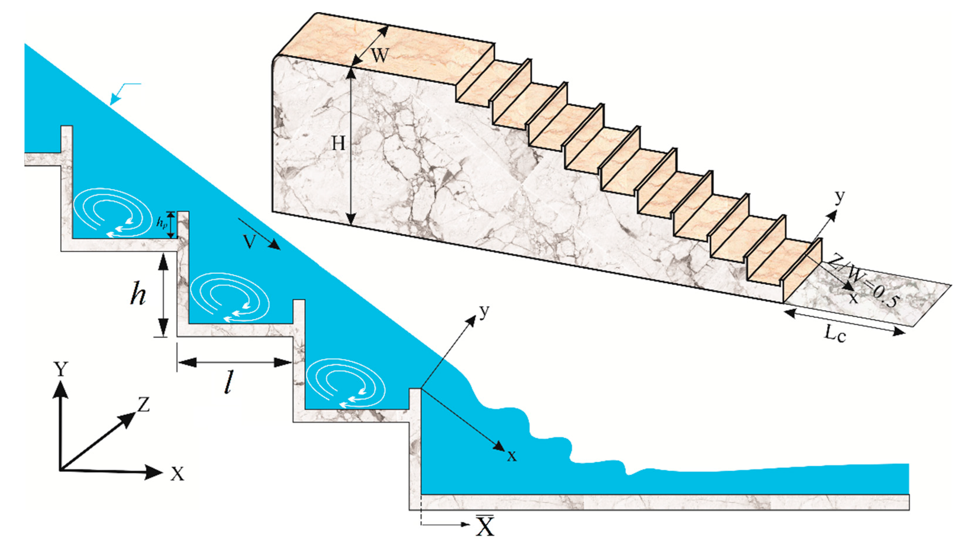
The objective of this work is, therefore, to develop the geometric and hydraulic parameters to prioritize and predict their effects on chute performance. Herein, a 3D numerical model developed by Morovati et al. [3] is employed. The results of the 3D simulations were then used to develop two regression models for predicting depth-averaged velocity (V_d) at the last step and critical length (L_c) at the downstream where maximum velocity occurs (see Figure 2). Additionally, the influence of each parameter on the chute performance is prioritized based on the data yielded by the developed numerical and regression models. Then, by utilizing these results, shear stress pattern in the last step, sidewalls, and downstream are produced and analyzed.

2. Materials and Methods

2.1. Numerical Model

A 3D numerical model developed by Morovati et al. [3] was adopted for the present work purposes. Detailed information on the employed numerical model in terms of meshing, mesh convergence analysis, governing equations, and boundary conditions considered for turbulence model and walls is found in Morovati et al. [3], and thus only a summary is provided here. The conducted simulations enjoy RANS equations, which were solved using the finite-volume method, and all equations were formulated with area and volume porosity functions using the fractional area/volume obstacle representation (FAVOR) approach to model complex geometric regions [36]. The renormalization-group (RNG) method that was employed in this study has broad applicability and is known to describe more accurately the flows characterized with areas of strong shear forces [36]. Advection in the conducted simulations was completed using the second-order upwind method for the discretization scheme. The Courant–Friedrichs–Lewy (CFL) value and the Krylov subspace dimension were set at <0.6 and 15, respectively, and the CFL < 0.6 was maintained by automatically adjusting the lengths of the time steps [3]. Results are presented at the condition concerning the final steady-state throughout the simulations implemented in this paper. The simulation time for the implemented runs employing a workstation with 24 cores and 32G of RAM was one to three days.

The free surface boundary conditions must be clearly defined for an accurate assessment of the free-surface dynamics. Subsequently, considering the free surface or sharp interface option, the volume of fluid (VOF) method was used in this study to evaluate these conditions with a single-fluid approach [36]. In addition, the actual physical situation should be modeled as closely to the real-world conditions as possible. This is important to make sure the results predicted are accurate to what is observed. Subsequently, specific discharge with the upstream total head for inlet, the outflow boundary condition for outlet, specified pressure for top, and wall boundary for the bottom and side walls were applied.

The computational domain was defined using hexahedral cell and multi-block technique. Six blocks were defined in which a uniform distribution of cells was considered in the transverse direction, i.e., Z direction. For the chute blocks, a uniform distribution of cells was considered in the X and Y direction, while for the upstream and downstream blocks, variable-sized cells were applied in X and Y directions so that, at the shared planes with the chute blocks, the cell sizes remained constant and as the distance from the last step and chute crest increased, the cell size in the X direction increased. For more information, refer to Morovati et al. [3].

In employing $k-\epsilon \left(RNG\right)$ turbulence closure, the values for shear stress, turbulence kinetic energy k, and dissipation rate $\epsilon$, were calculated using wall functions. Therefore, y⁺ values remained at the logarithmic region for the cells at the boundary layer, i.e., $y^{+}\in \left[35,300\right]$.

Table 1. Geometry properties of the stepped chutes adopted in the present study. NS is the number of steps.

References	S	l (m)	h (m)	H (m)	W (m)	NS
Felder et al. [6]	$8.9°$	0.319	0.05	1.05	0.5	21
Thorwarth [7]	$14.6°$	0.192	0.05	1.3	0.5	26
Gonzalez [10]	$21.8°$	0.25	0.1	1	1	10
Felder et al. [15]	$26.6°$	0.2	0.1	1	0.52	10
Morovati and Eghbalzadeh [32]	$30°$	0.173	0.1	1	0.52	10

provides information about the adopted stepped chutes in the present work. For each step chute, the uniform discharges were considered at the beginning of the computational domain and reached the chutes through a broad-crested weir followed by identical steps.

2.2. Design of Experiment

Design of experiment (DOE) is an effective method to understand a process as opposed to observing a process. Studying the influence of input parameter(s) on the response(s) is highly essential in a process, especially when different options are available for design [37,38,39,40]. Hence, DOE was applied by selecting the response surface methodology (RSM) based on the mixed-level full factorial design. This efficient method of DOE can also be used for modeling and optimizing processes [40,41]. Therefore, some important geometric and hydraulic parameters dominating over stepped chutes were developed in relation to experimental models employing high accurate 3D numerical model [3]; then, results were used as input parameters for the DOE model (

Table 2. The input parameters used for DOE together with their levels.

Input Parameters	Level 1	Level 2	Level 3	Level 4	Level 5
Chute slope $S$(S = tan$\theta$)	$8.9°$	$14.6°$	$21.8°$	$26.6°$	$30°$
Discharge Q (m3/s)	0.049	0.075	0.113	0.1641	0.2195
Pool height hp (m)	0	0.03	0.06	0.1	-
Chute height H (m)	1	1.5	2	-	-
Chute width W (m)	0.5	1	-	-	-

). The input parameters are chute slope S, discharge (Q), pool height (h_p), chute height (H), and chute width (W). The responses are depth-averaged velocity V_d (m/s) at the last step and critical length L_c (cm). Table 2 lists these input parameters along with their respective levels. The full factorial design based on the user-defined option resulted in 600 CFD runs $\left(5^2\times 4^1\times 3^1\times 2^1\right)$.

The levels given in Table 2 were selected based on real-world constructed examples. The range considered for H, Q, S, and h_p is representative of some stepped chutes used as waterways in rivers, drop structures, and transmission channels (see Guenther et al. [42]). For a chute width W that is greater than the range considered, there are practical examples that exist; however, such cases are more applicable for embankment dams and spillways, which are not the focus of the present study. Additionally, larger pool heights, i.e., h_p > 0.1 m, can cause problems associated with sediment accumulation and stability in the long term. Regarding discharge Q, since the flow regime passing on stepped chutes may change over time, the discharge ranges were chosen in a way that three types of flow regimes governing the chute, including nappe, transition, and skimming, are formed. It should be noted that the developed cases based on chute height H were performed in such a way that only the step height h was changed, i.e., l remained unchanged. In addition, in all cases, the number of steps in the 3D numerical model implemented based on the levels presented in Table 2 was similar to the experimental ones given in Table 1. For example, for H = 1.5 in the stepped chute with a slope of ${26.6}^{\mathrm{o}}$, the step height was changed from 0.1 m to 0.15 m.

This design allows researchers to analyze responses at whole combinations of the input parameters levels. Here, all significant parameters and their interactions have a 95% confidence interval level or a probability value less than 0.01 (p-value < 0.05) towards the responses. The analysis of variance (ANOVA) was also used to investigate the statistical significance of input parameters on the responses. Design Expert 10.0.4.0 and Minitab^® 18.1 were employed to analyze the results.

3. Results and Discussion

3.1. Model Development

Two-factor interaction (2FI) models suggested by the software were developed to predict V_d and L_c as responses. All main parameters and their interactions with the probability value less than 0.05 (p-value < 0.05) were considered as significant parameters. According to ANOVA results presented in

Table 3. ANOVA of the 2FI model for prediction of V_d response.

Source	Sum of Squares	df	Mean of Square	F-Value	p-Value	Significance
Model	428.18	9	47.13	1157.31	<0.0001	Significant
$S$	74.68	1	76.68	1833.81	<0.0001	Significant
Q	179.87	1	179.87	4416.80	<0.0001	Significant
hp	11.62	1	11.62	285.40	<0.0001	Significant
H	18.51	1	18.51	454.53	<0.0001	Significant
W	91.71	1	91.71	2251.86	<0.0001	Significant
$S\times$Q	7.72	1	7.72	189.46	<0.0001	Significant
$S\times$hp	46.70	1	46.70	1146.69	<0.0001	Significant
Q$\times$hp	0.4818	1	0.4818	11.83	0.0006	Significant
Q$\times$H	0.3284	1	0.3284	8.06	0.0047	Significant
Residual	24.03	590	0.0407
Corrected Total	448.21	599
R2	0.9464
Adjusted R2	0.9456
Predicted R2	0.94444
Adeq Precision	178.6339
PRESS	24.91
C.V.%	6.18

for the V_d response, all main parameters are highly significant. The ANOVA results in

Table 4. ANOVA of the 2FI model for prediction of L_c response.

Source	Sum of Squares	df	Mean of Square	F-Value	p-Value	Significance
Model	440,500	11	40,045.94	1012.23	<0.0001	Significant
$S$	13,118.66	1	13,118.66	331.60	<0.0001	Significant
Q	220,800	1	220,800	5579.91	<0.0001	Significant
hp	1337.61	1	1337.61	33.81	<0.0001	Significant
H	107.91	1	107.91	2.73	0.0992	Insignificant
W	180,000	1	180,000	4549.63	<0.0001	Significant
$S\times$Q	2737.68	1	2737.68	69.20	<0.0001	Significant
$S\times$hp	363.98	1	363.98	9.20	0.0025	Significant
$S\times$H	12,140.08	1	12,140.18	306.86	<0.0001	Significant
$S\times$W	499.18	1	499.18	12.62	0.0004	Significant
Q$\times$hp	2361.69	1	2361.69	59.70	<0.0001	Significant
Q$\times$W	20,153.37	1	20,153.37	509.41	<0.0001	Significant
Residual	23,262.61	588	39.56
Corrected Total	463,800	599
R2	9498
Adjusted R2	9489
Predicted R2	9480
Adeq Precision	143.2464
PRESS	24,126.92
C.V.%	10.38

for L_c show that all main parameters are significant towards the response except for the H parameter with a p-value of 0.0992. Since the interaction of this main parameter is significant, it is not possible to remove the H parameter from the initial model [43]. As can be seen in Table 4, the interaction of $S$-H has a p-value of less than 0.0001; then, the H parameter was kept in the final model for the prediction of L_c. For both models, insignificant interactions were removed from the initial models. Therefore, the final improved 2FI models were obtained according to the following equations:

$$\begin{gathered} V_d=2.34+0.03\times S+12.87\times Q-21.15\times h_p+0.31\times H-1.56\times W-0.24\times S\times Q+0.98\times S\times h_p \\ -12.47\times Q\times h_p+0.93\times Q\times H \end{gathered}$$

(1)

$$\begin{gathered} L_c=52.52-0.7\times S+642\times Q-129\times h_p-28.78\times H-10.87\times W-4.5\times S\times Q+2.7\times S\times h_p \\ +1.43\times S\times H-0.47\times S\times W+0.8728\times Q\times h_p-377.3\times Q\times W \end{gathered}$$

(2)

The Equations (1) and (2) developed are based on real-world factors and conditions. they can be used to predict responses for given levels of each factor but cannot determine the relative significance of each factor. To find the relative importance of the design factors, all analysis and model fittings need to be performed using coded design variables [43]. In the coded design variable, i.e., −1 ≤ x_i ≤ +1, the magnitudes of the model coefficients are directly comparable, that is, they are all dimensionless, and they measure the effects of changes in a design factor over a one-unit interval. In this study, each independent parameter was coded as x_i according to Equation (3) [40]:

$$x_i=\left(X_i-X_0\right)/\mathsf{\Delta }X$$

(3)

where X₀ is the value of X_i (selected parameters) at the center point, and ΔX denotes the step change. In addition, depth-averaged velocity V_d and critical length L_c as response data were normalized by dividing their actual value into a mean value of 2.3 (m/s) and 58 (cm), respectively. The final developed models obtained in terms of coded factors and normalized response are as follows. It is noteworthy that all parameters are unitless.

$$\begin{gathered} (V_d/2.3)=1.44+0.21\times S+0.33\times Q-0.083\times h_p+0.095\times H-0.17\times W-0.093\times S\times Q \\ +0.22\times S\times h_p-0.023\times Q\times h_p+0.017\times Q\times H \end{gathered}$$

(4)

$$\begin{array}{l}(L_c/58)=1.05+0.11\times S+0.46\times Q+0.036\times h_p-0.00902\times H-0.30478\times W-0.06978\times S\times Q\\ +0.024783\times S\times h_p+0.129705\times S\times H-0.02147\times S\times W+0.064143\times Q\times h_p\\ -0.13865\times Q\times W\end{array}$$

(5)

The coded equation helps to detect the relative impact of the factors by comparing the absolute value of factor coefficients [37]. In this regard, the descending order from highest to lowest significant factors on the response is as follows: Q > ($S$ × h_p) > $S$ > W > H > ($S$ × Q) > h_p > (Q × h_p) > (Q × H) for the depth-averaged velocity ($V_d$) and Q > $S$ > h_p > H > W > $S$ × Q) > ($S$ × h_p) > ($S\times$H) > ($S$ × W) > (Q × h_p) > (Q × W) for the critical length ($L_c$).

Prioritizing the effects of parameters is of great importance in recognizing the structure’s behavior and the design aspects. Table 3 and Table 4 give information regarding the impact of each parameter employing ANOVA results. Regarding V_d response, the highest important parameter is Q with an F-value of 4416.80, followed by W, $S$, H, and h_p, as presented in Table 3. In other words, the Q and h_p parameters have the highest and lowest impacts on the V_d response, respectively. This order also remained constant for L_c response except for H and h_p, in which H has the lowest impact. For both responses, W as a geometric parameter plays a significant role in V_d and L_c. For both responses, H and h_p parameters have an insignificant impact compared to the other three parameters; however, this effect is more pronounced for the L_c response. According to ANOVA results presented in Table 3 and Table 4, the model’s F-values of 1157.31 and 1012.23 (p-value < 0.0001) for V_d (m/s) and L_c (cm), respectively, show that the final 2FI models are highly significant and fairly appropriate for the present results.

3.2. Statistical Validation of Regression Models

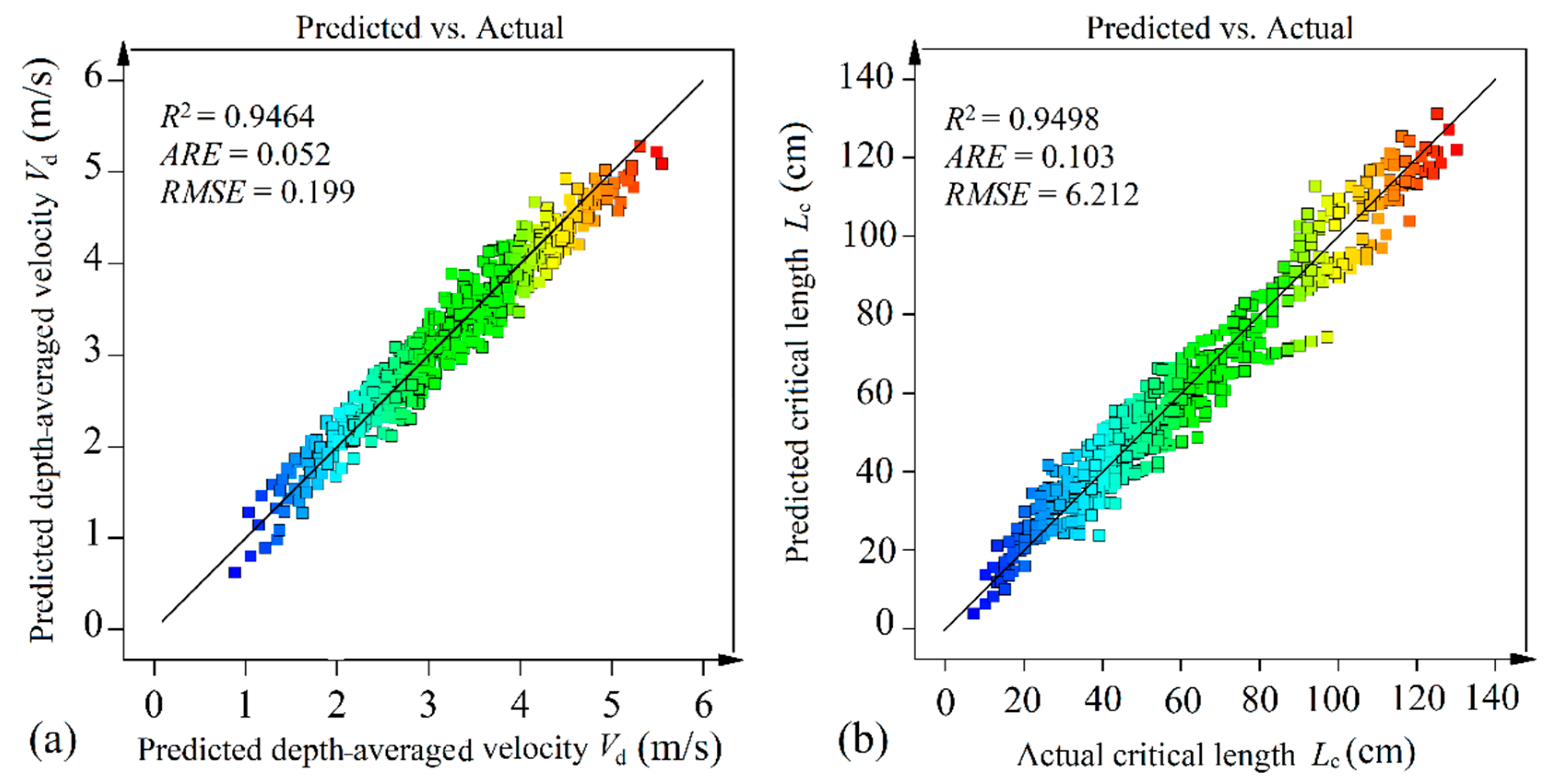
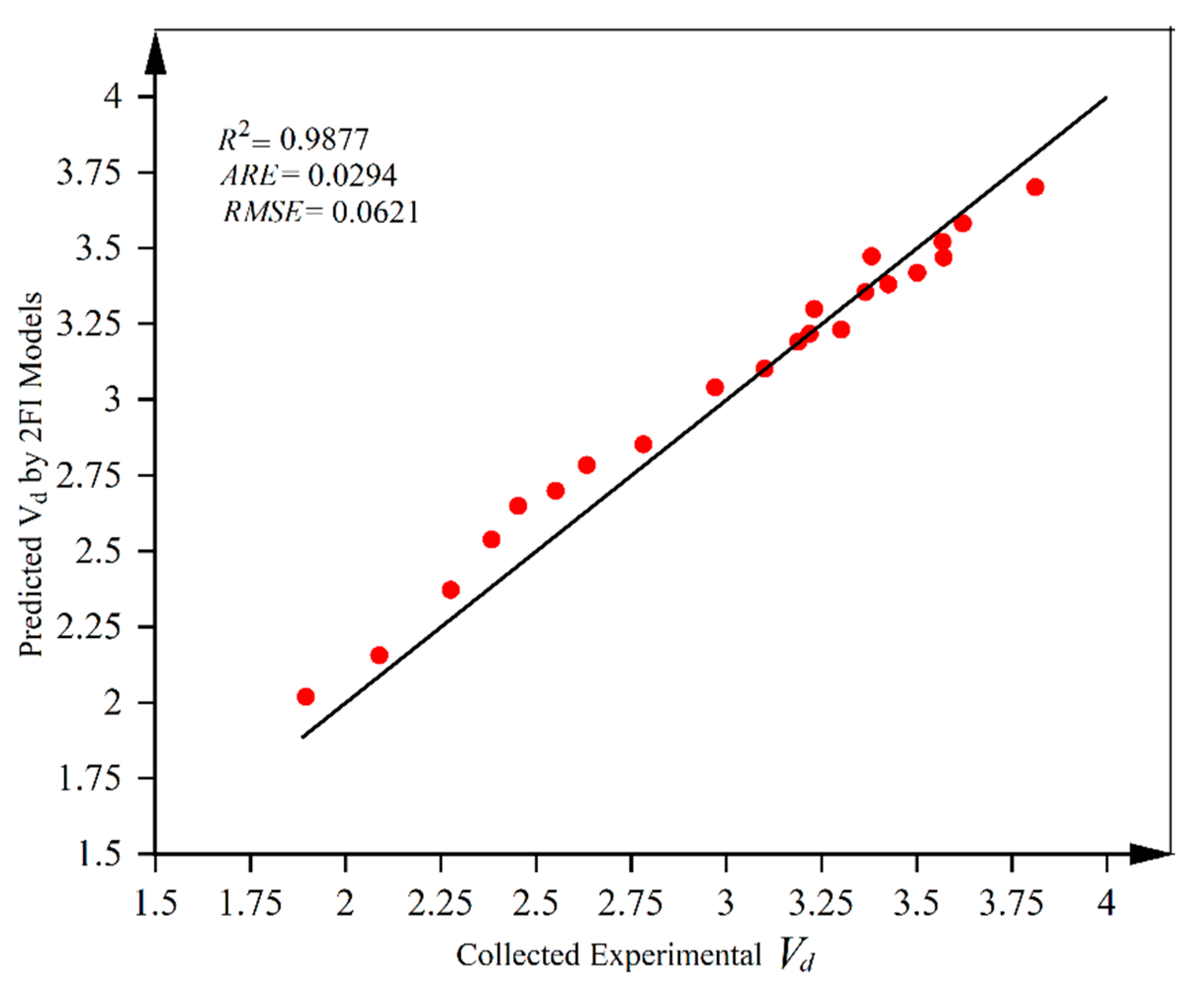
After identifying the significance of parameters and developing the regression models, it is important to validate the models and evaluate their accuracy. Hence, four main approaches were selected: (1) plot of the predicted data versus simulated data, (2) normal probability plot, (3) plot of residuals vs. run order, and (4) plot of residuals versus predicted data. Figure 3a,b illustrates the predicted data by 2FI models against the simulated data together with the absolute relative error (ARE) and root mean square error (RMSE) to verify the ability of the models for the prediction of the response. The formulas for the statistical measures, coefficient of determination (R²), as well as adjusted and predicted R² are listed in

Table 5. Performance relations ^a.

$R^2=1-\frac{{{\displaystyle \sum }}_{i=1}^N{\left(Act.Y_i-Pred.Y_i\right)}^2}{{{\displaystyle \sum }}_{i=1}^N{\left(Act.Y_i-Avg.Y\right)}^2}$

$Adjusted R^2=1-R^2\left(\frac{n-1}{N-k-1}\right)$

$Predicted R^2=1-\left(\frac{Press}{Corrected Total}\right)$

$ARE=\left|\frac{Act.Y-Pred.Y}{Act.Y}\right|$

$RMSE={\left[\frac{{{\displaystyle \sum }}_{i=1}^N(Act.Y-Pred.Y}{N}\right]}^2$

^a In above relations, N, K, Act. Yi, and Pred. Yi are the number of data in the dataset, the number of terms in the model, the i-th actual value, and the i-th model prediction value, respectively.

.

Figure 3a,b shows the close proximity of the model prediction with the simulated data demonstrating the validity of 2FI models. From Figure 3 and Table 3 and Table 4, the R² was found to be almost 0.95, which is close to 1, indicating that the models can explain 95% of the variability in response, and the predicted data from the 2FI models agree well with the simulated data. Sometimes a model includes several independent parameters and the interaction terms; in such cases, in order to measure the quality of the model, it is fair to consider the adjusted R² [43]. In addition, the difference between the predicted R² and the adjusted R² values should be less than 0.2. As seen in Table 3 and Table 4, both V_d and L_c results show reasonable agreement between the predicted R² and the adjusted R² with a difference of less than 0.001.

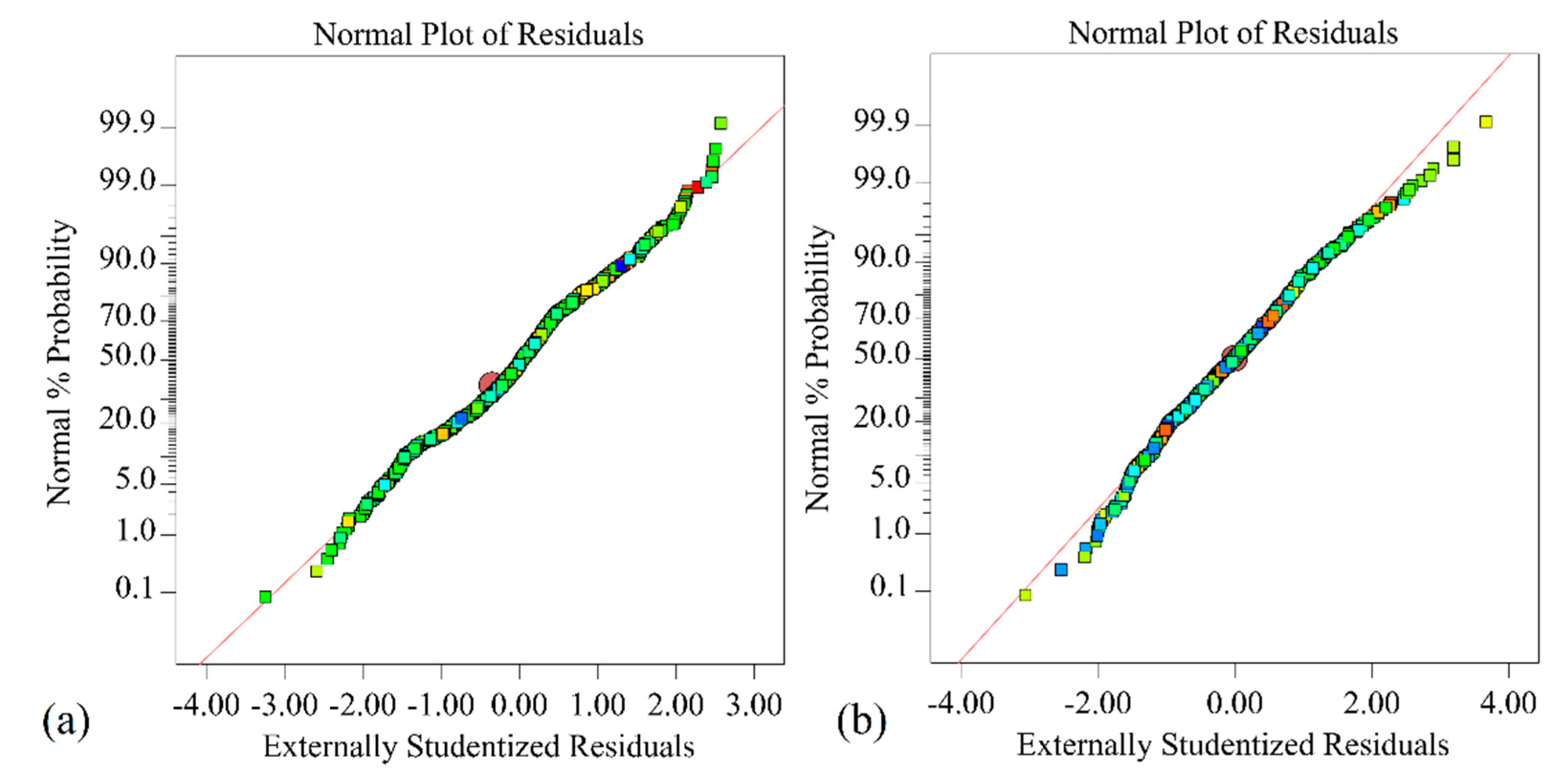
As an additional step for model validation, it is necessary to compare the probability to residuals and residuals to the run order. The normal probability plots are used to identify whether the data follows a normal distribution. As shown in Figure 4, the points fall along the reference line, and there is no kurtosis or significant variation in the sample distributions, indicating the normal distribution of data.

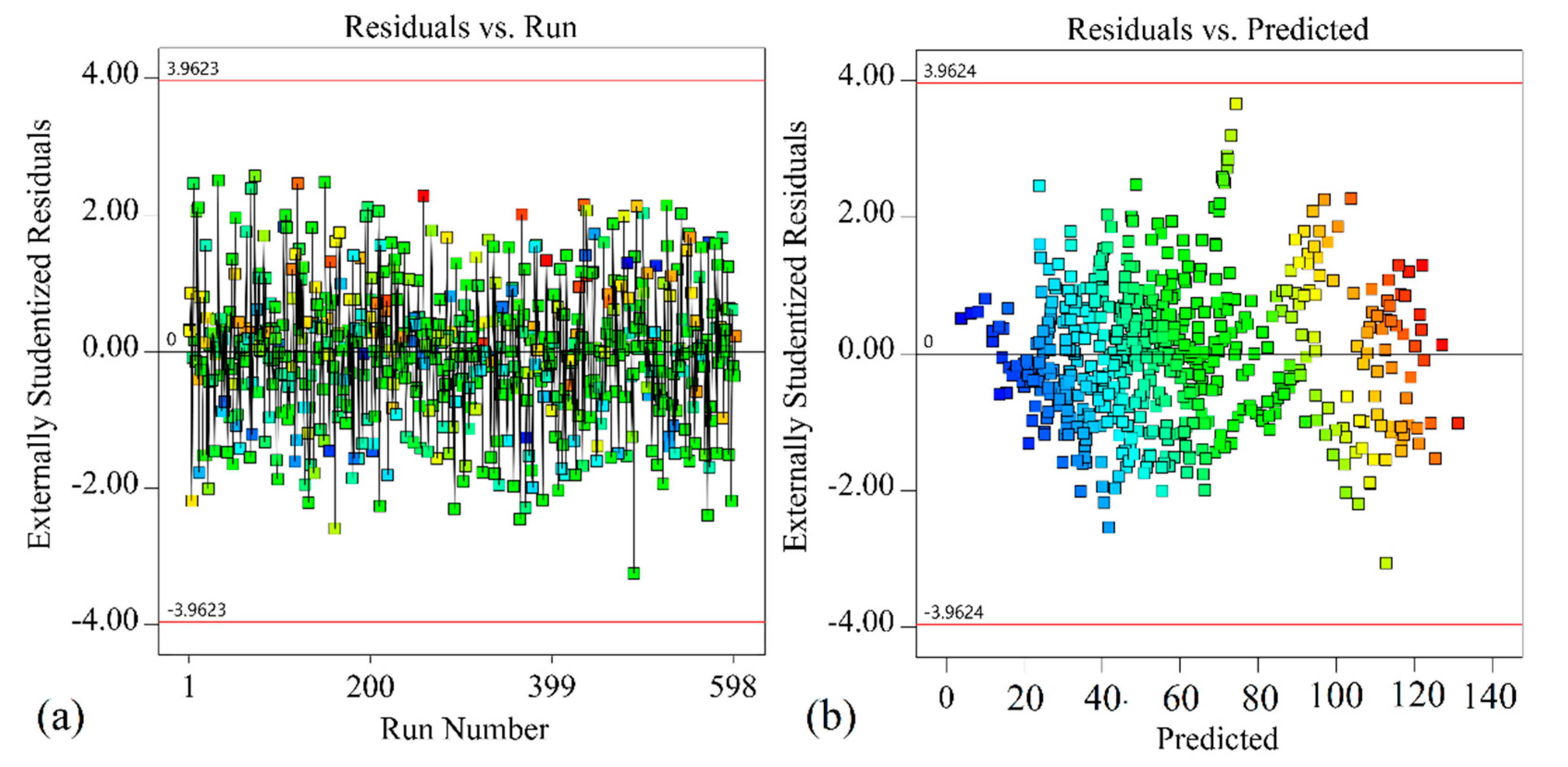
The plot of externally studentized residuals is an effective method to detect the outlier data since externally studentized residuals are more sensitive to detect outliers as compared to internally studentized residuals. According to Figure 5a, the discrepant data and potential outliers are not detected in the actual data for V_d. Figure 5b also displays the externally studentized residuals versus predicted values for L_c. The plot ideally exhibits a constant variation from the left (low level of response) to the right (highest predicted level), and no outlier data are detected. Similar results were obtained for the externally studentized residuals versus predicted values for V_d, and externally studentized residuals versus run for L_c.

In order to evaluate the performance of the model further, the data available from the literature that have different geometry and hydraulic characteristics in relation to what were considered as input parameters (see Table 2) were compared with the data predicted by the 2FI model. Figure 6 shows the scatter plot of the results obtained from the 2FI model and the actual data reported by Felder et al. [6,15]. The values of the statistical measures presented in Figure 6 indicate that the given 2FI model enjoys a high capability of predicting V_d, even with the geometry and hydraulic changes; however, these changes should be in the range presented in Table 2.

3.3. Main Impact of Factors and Their Interaction Effects

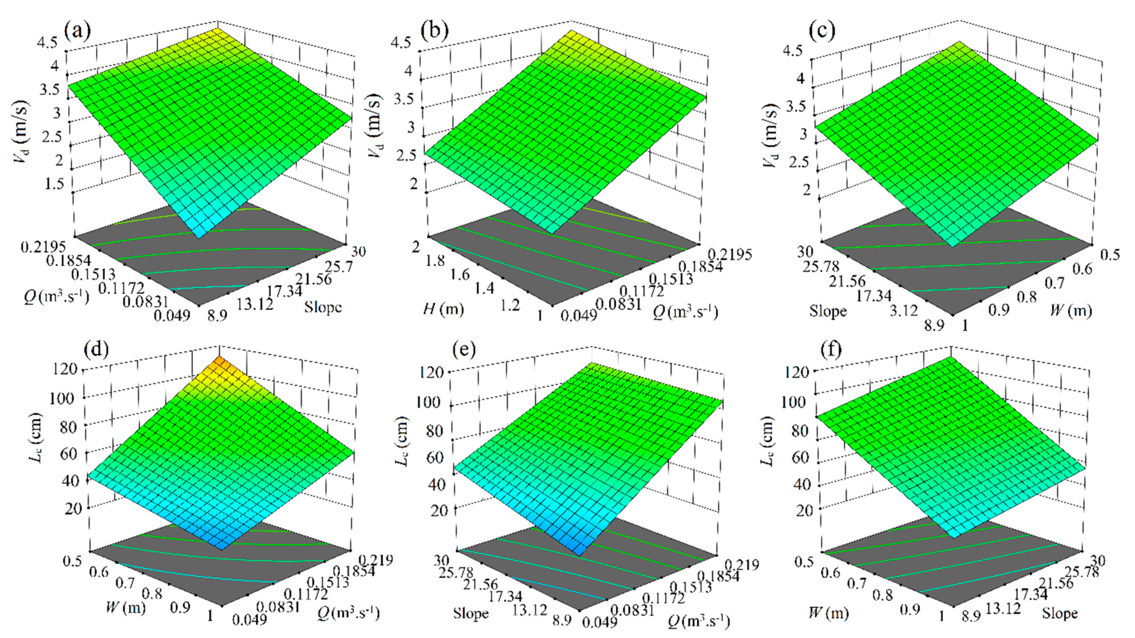
In Table 3 and Table 4, the parameters’ impacts were prioritized, although the effects of the parameters on the responses are difficult to understand. Therefore, the 3D surface plots are provided to better illustrate the parameter’s impact on the V_d and L_c responses. Here, these plots are presented through data obtained by the 2FI models with two parameters (the three other parameters were fixed at their specific values, i.e., $S=20°$, Q = 0.1342 m³/s, h_p = 0.05 m, H = 1.5 m, and W = 0.75 m). Figure 7a,b demonstrates the effects of Q, $S$, and H parameters on the V_d. In both figures, the simultaneous increase of the parameters increases the responses, with the difference that the slope of $S$ is higher than H, resulting in a more significant increase. There is a different behavior pattern for the impact of $S$ and W on the V_d response; for example, for the minimum value of V_d, W should increase while the $S$ needs to be decreased (Figure 7c). Such a similar pattern also exists in the case where L_c forms near the last step; however, this seems not to be a cautious approach since high velocity exiting the area after the last step can cause scouring and breach formation, undermining the stability of the structure. Moreover, a comparison of W and $S$ parameters in Figure 7f indicates that W plays a more significant role in controlling the location of maximum velocity at the downstream. Therefore, according to the results presented in Table 3 and Table 4 and Figure 7, W can be regarded as the most important geometric parameter influencing V_d as well as L_c.

When there is more than one variable in a process, the interaction between the factors may occur. There is interaction when one variable’s impact on the response relies on the level of another variable. The DOE method’s strength is the management of interactions amongst variables [37].

As shown in Equations (1) and (2) and as evidenced by Table 3 and Table 4, there are interactions between the factors. The significant interaction terms are $S\times Q$, $h_p$, $Q\times h_p$, and $Q\times H$ in Equation (1), while in Equation (2), $Q$, $S\times h_p$, $S\times H$, $S\times W$, $Q\times h_p$, and $Q\times W$ are significant interaction terms. The interactions between the factors can be established using an interaction graph to display any two-factor interactions. These figures illustrate the response as a function of one variable with the two different levels of the other variable while the remaining independent variables are kept constant. In such plots, the nonparallel lines demonstrate that an interaction exists between the two factors (the details on the interaction evaluation are provided in Mathews [37]). Two of such interaction terms are highlighted and discussed in the subsequent paragraphs.

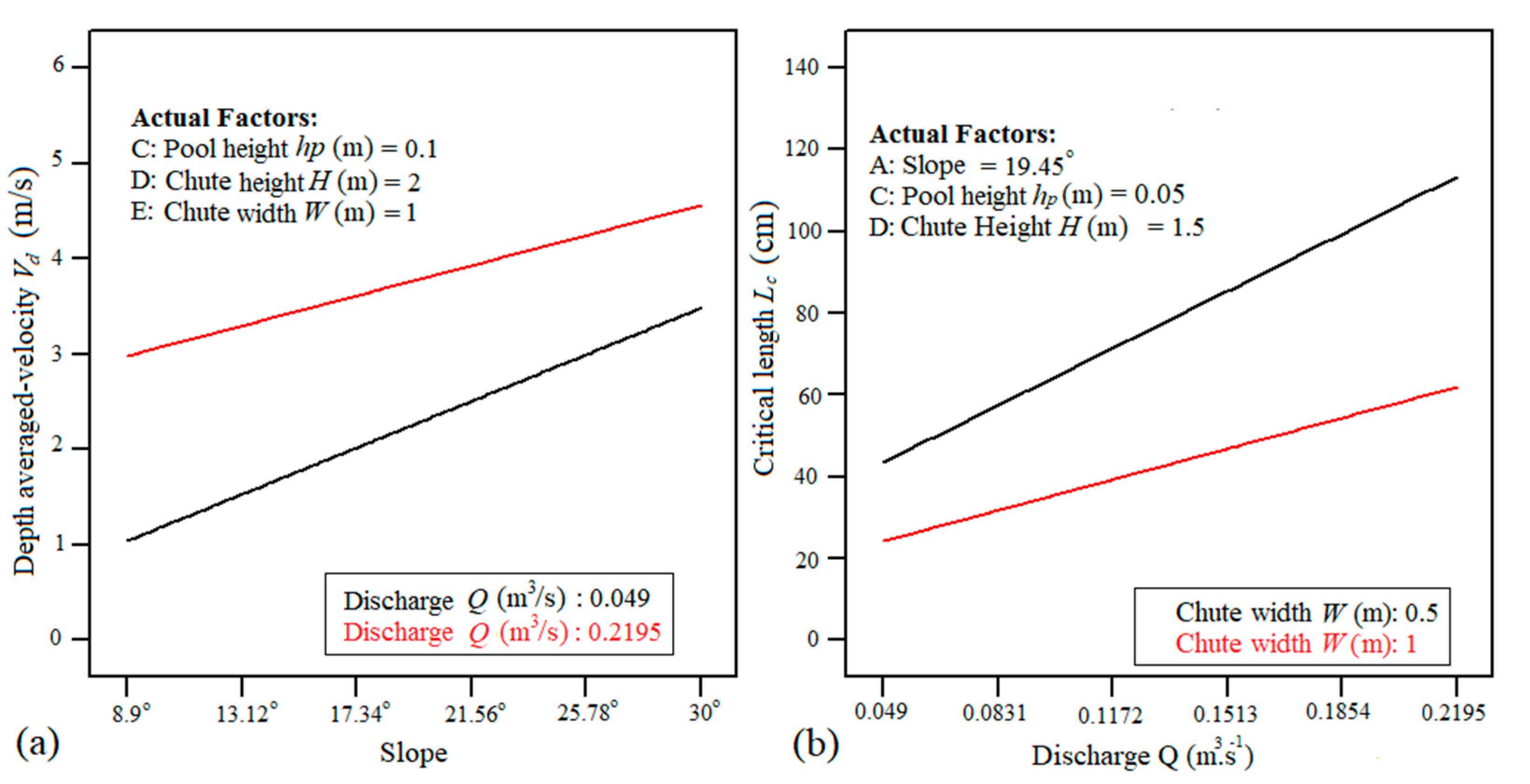
The interaction between the discharge (Q) and slope ($S$) and its impact on the depth-averaged velocity is shown in Figure 8. Depending on the discharge value Q, the stepped chutes experience fully developed or partially developed hydraulic jumps in lower discharges, coherent stream in higher discharges, and cavities above the steps and the corner created between the last step’s height and downstream bottom [44,45]. These features play a significant role in passing flow in terms of decreasing flow velocity and can be changed if the geometry and hydraulic characteristics are altered. Figure 8a shows that V_d varies as the Q changes on each slope, with more pronounced variations attributed to slope $8.9°$. On slope $8.9°$ and for the discharge range given in Table 1, i.e., 0.049 < Q (m³/s) < 0.2195, the chute experiences nappe, transition, and skimming flow regimes while for stepped slope, i.e., $30°$, a skimming flow regime forms (see Chanson [44]). This implies that the more significant variation of V_d is attributed to the changes between various flow regimes, i.e., nappe to skimming, than the changes in Q within the limit of a flow regime, i.e., skimming. The interaction between the chute width (W) and discharge (Q) and its impact on critical length is illustrated in Figure 8b. As seen, changing the chute width W as a factor changing the flow regime causes significant differences for L_c, especially in greater discharges. According to Equation (6), as the chute width W increases at a constant discharge Q, the flow depth passing over the chute decreases. As a result, cavities and hydraulic jumps’ properties are likely influenced because their formation directly depends on hydraulic and geometric properties [6,15,44,45].

$$\frac{Q}{W}=\left(0.92+0.153\times \frac{H_1}{L_{crest}}\right)\times \sqrt{g\times {\left(\frac{2}{3}\times H_1\right)}^3}$$

(6)

where H₁ and L_creast represent the flow depth above chute crest and crest length, respectively. The results presented in Figure 8b, where the chute width increases from 0.5 to 1 m, indicate that the critical length L_c is almost halved for all discharge. Such a decrease appears to be due to (1) the flow depth decreasing as discussed earlier, and thus the critical length occurs at a shorter distance from the last step, and also (2) the decreased flow depth, which likely results in changes in the flow regime as well as the size of the vortices above the steps and at the downstream.

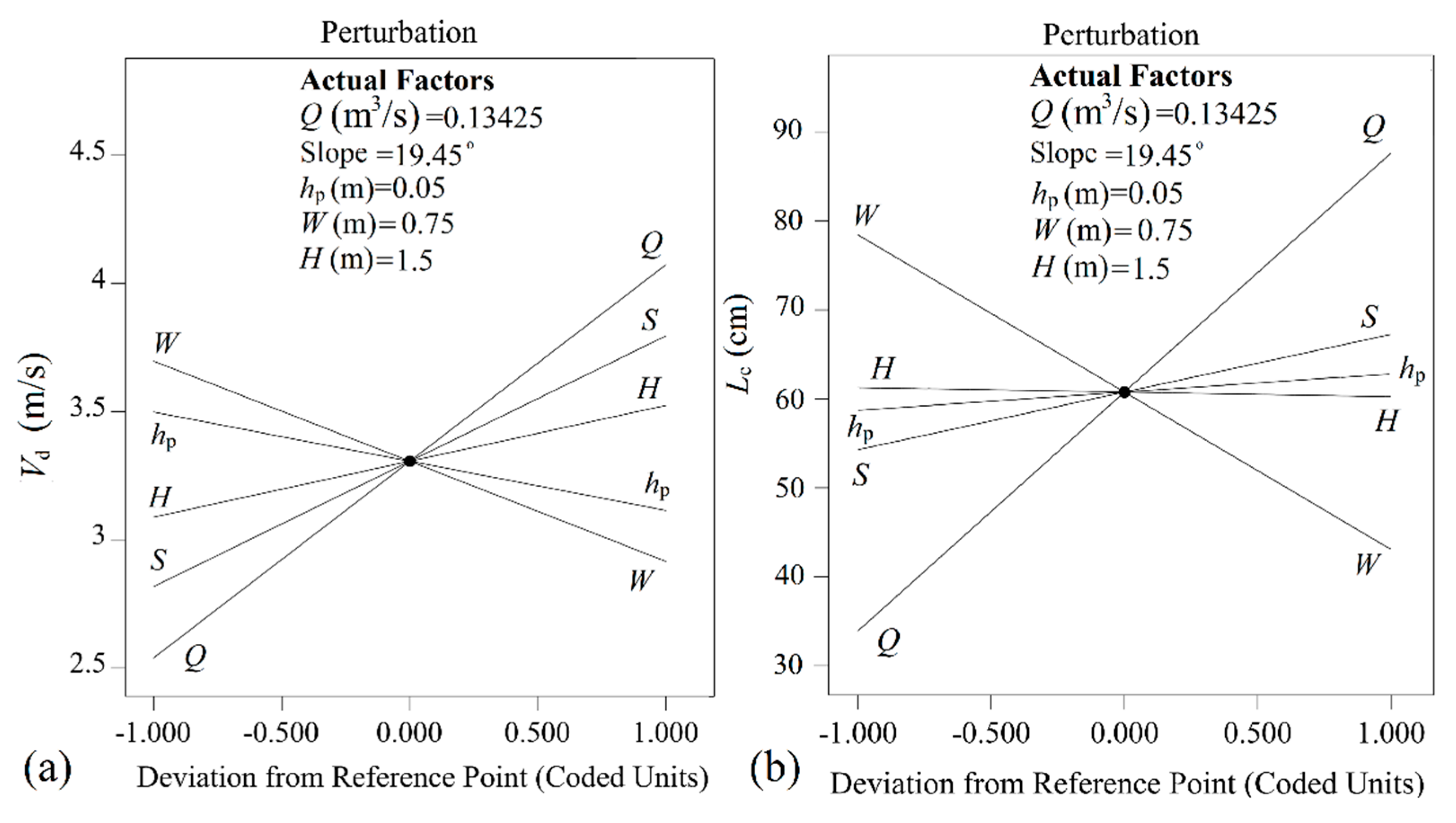
The perturbation plot compares the effects of all parameters at a specific value as well as at the optimum conditions in the design space. Design-Expert sets the reference point default at the middle of the design space (the coded zero level of each parameter). The response is plotted by changing only one parameter over its range while holding all the other parameters constant. The perturbation plots for the V_d and L_c are displayed in Figure 9a,b, respectively. All parameters experience a linear effect on the V_d and L_c responses. When the slope of the line is sharper, it means that the parameter has a more significant impact on the response. Both the V_d and L_c responses are controlled mainly by Q and W parameters, which significantly impact these responses. Two slopes are observed for lines, positive and negative, which means that if the slope of the line is positive, increasing the corresponding parameter to that line would increase responses, but for negative slope, as the parameter increases, the values for responses decreases (for example, see W and Q for L_c). According to the parameters’ values shown, both h_p and H have an insignificant impact in determining the critical length at the downstream. Additionally, the discharge Q of natural waterways varies constantly as it is affected by many environmental factors. If we assume the geometric parameters are constant, the length of the critical area of the downstream can be calculated based on a given range of discharge values, for example, the minimum and maximum values.

3.4. Shear Stress

With the help of Equation (2), the critical length at the downstream was measured. The shear stress pattern at the edge of the last step, the sidewalls, and downstream where the maximum velocity occurs (L_c) is displayed in Figure 10 for different slopes and discharges. The shear stress pattern is almost symmetrical in all cases, although there are some insignificant differences. For lower slopes, i.e., $8.9°$ and $14.6°$, the maximum shear stress occurs on the sidewalls, while in the higher slopes, sidewalls and step surfaces experience approximately identical shear stress. The shear stress pattern on the sidewalls differs between steeper and lower slopes. For lower slopes, the pattern on the sidewalls forms a parabolic distribution with the maximum stress occurring near the middle of the flow depth. For steeper slopes, the pattern on the sidewalls forms an approximately linear distribution with the maximum stress near the base where the sidewalls and step surface intersect. The shear stress distribution at the downstream showed some similarities and small changes in each case. The most significant difference observed was the location of the maximum shear stress value. With higher slopes, the maximum shear stress occurred at the downstream, while for lower slopes, the maximum value was recorded on the sidewalls. Therefore, with increasing slope, the location of the maximum shear stress changes from the sidewall of the last step to the downstream. It should be noted that the results shown in Figure 10 correspond to the flat stepped chutes, i.e., h_p = 0.

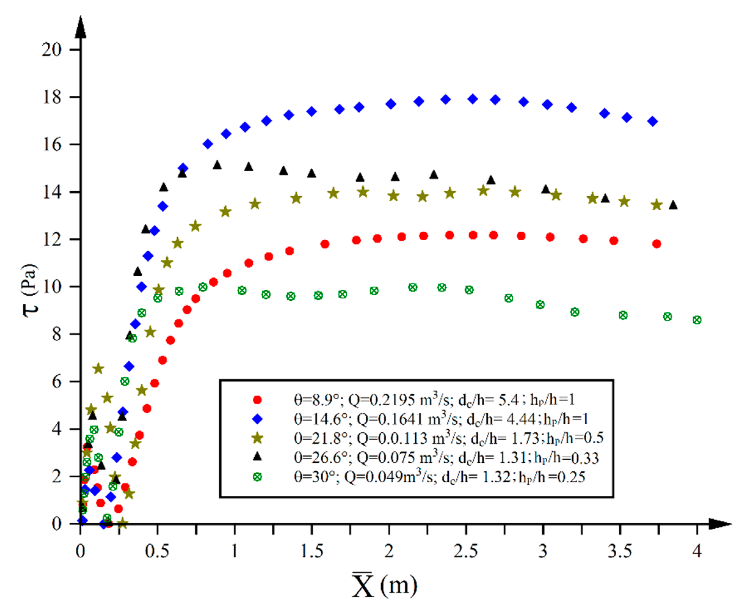
Figure 11 illustrates the shear stress distribution along downstream immediately after the last step at Z/W = 0.5 for different slopes and discharges. The significant variation of shear stress occurs at the area close to the last step, although the values of shear stress in this area are much smaller than the rest of the downstream. After this area, the shear stress sharply increases, followed by an insignificant variation for the rest of the downstream. A comparison of the results highlights the point that the changing pattern of the shear stress seems to be independent of geometric and hydraulic characteristics since almost a similar pattern is seen for all cases; however, these characteristics may impact shear stress values.

4. Conclusions

This work was conducted to investigate and prioritize the influence of geometric and hydraulic parameters on chute behavior. Five important parameters were selected: slope, discharge, pool height, chute height, and chute width. These parameters were then utilized to develop 600 cases, employing a highly accurate 3D numerical model. Results were used for RSM design, which resulted in two developed regression models for predicting V_d and L_c with coefficient determination (R²) of about 0.95, highlighting the high accuracy of the models. Employing the analysis of variance (ANOVA), prioritization of the influence of the studied parameters on the dynamic behavior of the investigated chutes was accomplished in which Q, W, $\theta$, H, and h_p had the most significant influence on V_d, respectively. The same order was also reported for L_c; however, h_p had greater influence than H. Results revealed that the H parameter played an insignificant role in detecting L_c and can be neglected. By employing the regression model for L_c, the shear stress distribution at the critical section of the downstream in terms of the maximum velocity was investigated and compared to that of the last step and sidewalls. For $\theta \le 14.6°$, the greatest value of shear stress was formed on the sidewalls compared to the last step and downstream; however, the difference between downstream and side walls was not significant as compared to the sidewalls and the last step’s edge. For $\theta \ge 21.8°$, the maximum shear stress was formed at the downstream, and the difference between the shear stress on the last step’s edge and side walls was not significant. Additionally, the shear stress in the longitudinal direction of the downstream showed that the behavior pattern of shear stress did not depend on the geometric and hydraulic parameters, and so an approximately similar pattern was observed in all cases. The findings in this study prove that these methods could effectively investigate and prioritize the parameters of a structure to improve the design and performance.

References

- Wang, Z.Y.; Lee, J.H.; Melching, C.S. River Dynamics and Integrated River Management; Springer: Cham, Switzerland, 2014. [Google Scholar]
- Valero, D.; Bung, D.B.; Crookston, B.M. Energy dissipation of a Type III basin under design and adverse conditions for stepped and smooth spillways. J. Hydraul. Eng. 2018, 144, 04018036. [Google Scholar] [CrossRef]
- Morovati, K.; Homer, C.; Tian, F.; Hu, H. Opening configuration design effects on pooled stepped chutes. J. Hydraul. Eng. 2021, in press. [Google Scholar] [CrossRef]
- Felder, S.; Chanson, H. Energy dissipation down a stepped spillway with nonuniform step heights. J. Hydraul. Eng. 2011, 137, 1543–1548. [Google Scholar] [CrossRef] [Green Version]
- Felder, S.; Chanson, H. Aeration, flow instabilities, and residual energy on pooled stepped spillways of embankment dams. J. Irrig. Drain. Eng. 2013, 139, 880–887. [Google Scholar] [CrossRef] [Green Version]
- Felder, S.; Fromm, C.; Chanson, H. Air Entrainment and Energy Dissipation on A 8.9 Slope Stepped Spillway with Flat and Pooled Steps; The University of Queensland: Brisbane, Australia, 2012. [Google Scholar]
- Thorwarth, J. Hydraulisches Verhalten der Treppengerinne mit eingetieften Stufen Selbstinduzierte Abflussinstationaritäten und Energiedissipation (Hydraulics of Poole Stepped Spillways—Self-induced Unsteady Flow and Energy Dissipation). Ph.D. Thesis, University of Aachen, Aachen, Germany, 2008. [Google Scholar]
- Kökpinar, M.A. Flow over a stepped chute with and without macro-roughness elements. Can. J. Civ. Eng. 2004, 31, 880–891. [Google Scholar] [CrossRef]
- Andre, S. High Velocity Aerated Flows on Stepped Chutes with Macro-Roughness Elements. Ph.D. Thesis, Laboratoire de Constructions Hydraulics, Lausanne, Switzerland, 2004. [Google Scholar]
- Gonzalez, C.A. An Experimental Study of Free-Surface Aeration on Embankment Stepped Chutes. Ph.D. Thesis, The University of Queensland, Brisbane, Australia, 2005. [Google Scholar]
- Meireles, I.; Matos, J. Skimming flow in the nonaerated region of stepped spillways over embankment dams. J. Hydraul. Eng. 2009, 135, 685–689. [Google Scholar] [CrossRef]
- Bung, D.B. Developing flow in skimming flow regime on embankment stepped spillways. J. Hydraul. Res. 2011, 49, 639–648. [Google Scholar] [CrossRef]
- Zhang, G.; Chanson, H. Hydraulics of the developing flow region of stepped spillways. I: Physical modeling and boundary layer development. J. Hydraul. Eng. 2016, 142, 04016015. [Google Scholar] [CrossRef] [Green Version]
- Zhang, G.; Chanson, H. Hydraulics of the developing flow region of stepped spillways. II: Pressure and velocity fields. J. Hydraul. Eng. 2016, 142, 04016016. [Google Scholar] [CrossRef] [Green Version]
- Felder, S.; Guenther, P.; Chanson, H. Air-Water Flow Properties and Energy Dissipation on Stepped Spillways: A Physical Study of Several Pooled Stepped Configurations; The University of Queensland: Brisbane, Australia, 2012. [Google Scholar]
- Felder, S.; Chanson, H. Energy dissipation, flow resistance and gas-liquid interfacial area in skimming flows on moderate-slope stepped spillways. Environ. Fluid Mech. 2009, 9, 427–441. [Google Scholar] [CrossRef]
- Dey, S.; Lambert, M.F. Reynolds stress and bed shear in nonuniform unsteady open-channel flow. J. Hydraul. Eng. 2005, 131, 610–614. [Google Scholar] [CrossRef]
- Chanson, H. Comparison of energy dissipation between nappe and skimming flow regimes on stepped chutes. J. Hydraul. Res. 1994, 32, 213–218. [Google Scholar] [CrossRef]
- Jiang, L.; Diao, M.; Xue, H.; Sun, H. Energy dissipation prediction for stepped spillway based on genetic algorithm–support vector regression. J. Irrig. Drain. Eng. 2018, 144, 04018003. [Google Scholar] [CrossRef]
- Khatibi, R.; Salmasi, F.; Ghorbani, M.A.; Asadi, H. Modelling energy dissipation over stepped-gabion weirs by artificial intelligence. Water Resour. Manag. 2014, 28, 1807–1821. [Google Scholar] [CrossRef]
- Baylar, A.; Hanbay, D.; Ozpolat, E. Modeling aeration efficiency of stepped cascades by using ANFIS. CLEAN–Soil Air Water 2007, 35, 186–192. [Google Scholar] [CrossRef]
- Laucelli, D.; Giustolisi, O. Scour depth modeling by a multi-objective evolutionary paradigm. Environ. Model. Softw. 2011, 26, 498–509. [Google Scholar] [CrossRef]
- Emiroglu, M.E.; Bilhan, O.; Kisi, O. Neural networks for estimation of discharge capacity of triangular labyrinth side-weir located on a straight channel. Expert Syst. Appl. 2011, 38, 867–874. [Google Scholar] [CrossRef]
- Azamathulla, H.M. Gene expression programming for prediction of scour depth downstream of sills. J. Hydrol. 2012, 460, 156–159. [Google Scholar] [CrossRef]
- Dursun, O.F.; Kaya, N.; Firat, M. Estimating discharge coefficient of semi-elliptical side weir using ANFIS. J. Hydrol. 2012, 426, 55–62. [Google Scholar] [CrossRef]
- Bagatur, T.; Onen, F. A predictive model on air entrainment by plunging water jets using GEP and ANN. KSCE J. Civ. Eng. 2014, 18, 304–314. [Google Scholar] [CrossRef]
- Roushangar, K.; Akhgar, S.; Salmasi, F.; Shiri, J. Neural networks-and neuro-fuzzy-based determination of influential parameters on energy dissipation over stepped spillways under nappe flow regime. ISH J. Hydraul. Eng. 2017, 23, 57–62. [Google Scholar] [CrossRef]
- Morovati, K.; Eghbalzadeh, A.; Javan, M. Numerical investigation of the configuration of the pools on the flow pattern passing over pooled stepped spillway in skimming flow regime. Acta Mech. 2016, 227, 353–366. [Google Scholar] [CrossRef]
- Li, S.; Zhang, J. Numerical investigation on the hydraulic properties of the skimming flow over pooled stepped spillway. Water 2018, 10, 1478. [Google Scholar] [CrossRef] [Green Version]
- Attarian, A.; Hosseini, K.; Abdi, H.; Hosseini, M. The effect of the step height on energy dissipation in stepped spillways using numerical simulation. Arab. J. Sci. Eng. 2014, 39, 2587–2594. [Google Scholar] [CrossRef]
- Morovati, K.; Eghbalzadeh, A. Stepped spillway performance: Study of the pressure and turbulent kinetic energy versus discharge and slope. J. Water Sci. Res. 2015, 8, 63–77. [Google Scholar]
- Li, S.; Yang, J. Effects of Inclination Angles on Stepped Chute Flows. Appl. Sci. 2020, 10, 6202. [Google Scholar] [CrossRef]
- Munta, S.; Otuna, J.A.; Abubakar, I. Prediction of inception length of flow over different stepped chute geometry. Nigerion J. Technol. 2015, 34, 631–635. [Google Scholar] [CrossRef] [Green Version]
- Bombardelli, F.A.; Meireles, I.; Matos, J. Laboratory measurements and multi-block numerical simulations of the mean flow and turbulence in the non-aerated skimming flow region of steep stepped spillways. Environ. Fluid Mech. 2011, 11, 263–288. [Google Scholar] [CrossRef] [Green Version]
- Morovati, K.; Eghbalzadeh, A. Study of inception point, void fraction and pressure over pooled stepped spillways using Flow-3D. Int. J. Numer. Methods Heat Fluid Flow 2018, 28, 982–998. [Google Scholar] [CrossRef]
- Flow Science. FLOW-3D User’s Manual. Version 10.1; Flow Science: Los Alamos, NM, USA, 2013. [Google Scholar]
- Mathews, P.G. Design of Experiments with MINITAB; ASQ Quality Press: Milwaukee, WI, USA, 2005. [Google Scholar]
- Akbari, S.; Mahmood, M.S.; Ghaedi, H.; Al-Hajri, S. New empirical model for viscosity of sulfonated polyacrylamide polymers. Polymers 2019, 11, 1046. [Google Scholar] [CrossRef] [Green Version]
- Rangkooy, H.A.; Ghaedi, H.; Jahani, F. Removal of xylene vapor pollutant from the air using new hybrid substrates of TiO2-WO3 nanoparticles immobilized on the ZSM-5 zeolite under UV radiation at ambient temperature. 2019, Experimental towards modeling. J. Environ. Chem. Eng. 2019, 7, 103247. [Google Scholar] [CrossRef]
- Murshid, G.; Ghaedi, H.; Ayoub, M.; Garg, S.; Ahmad, W. Experimental and correlation of viscosity and refractive index of non-aqueous system of diethanolamine (DEA) and dimethylformamide (DMF) for CO2 capture. J. Mol. Liq. 2018, 250, 162–170. [Google Scholar] [CrossRef]
- Ghaedi, H.; Ayoub, M.; Sufian, S.; Murshid, G.; Farrukh, S.; Shariff, A.M. Investigation of various process parameters on the solubility of carbon dioxide in phosphonium-based deep eutectic solvents and their aqueous mixtures: Experimental and modeling. Int. J. Greenh. Gas Control. 2017, 66, 147–158. [Google Scholar] [CrossRef]
- Guenther, P.; Felder, S.; Chanson, H. Flow aeration, cavity processes and energy dissipation on flat and pooled stepped spillways for embankments. Environ. Fluid Mech. 2013, 13, 503–525. [Google Scholar] [CrossRef] [Green Version]
- Montgomery, D.C. Design and Analysis of Experiments, 7th ed.; John Wiley & Sons: New York, NY, USA, 2008. [Google Scholar]
- Chanson, H. Self-aerated flows on chutes and spillways. J. Hydraul. Eng. 1993, 119, 220–243. [Google Scholar] [CrossRef] [Green Version]
- Chanson, H. Hydraulics of Stepped Chutes and Spillways; CRC Press: Boca Raton, FL, USA, 2002. [Google Scholar]
Figure 1.
The examples of stepped chutes constructed as (a) water transmission channel in Piranshahr, Iran on 12 April 2020 (photograph by Khosro Morovati), and (b) fishway structure on the Okura River, Japan on 9 October 2012 (photograph by Hubert Chanson with permission). The stepped channel consists of a staggered combination of flat and pooled steps.
Figure 2.
An example of stepped chute used in this study and measurement positions; h and l denote step height and step length, respectively; is the calculated distance from the vertical face of the last step along downstream.
Figure 3.
Predicted data vs. simulated data; (a) depth-averaged velocity Vd (m/s), and (b) critical length Lc (cm).
Figure 4.
Normal probability versus residuals for (a) depth-averaged velocity Vd (m/s), and (b) critical length Lc (cm).
Figure 5.
The plots of (a) residuals vs. ran for depth-averaged velocity Vd (m/s), and (b) residuals vs. predicted data for critical length Lc (cm).
Figure 6.
Comparison of predicted depth-averaged velocity (Vd) between 2FI model and re-analyzed data reported by Felder et al. [6,15].
Figure 7.
The surface plots for the Lc and Vd response as a function of (a,e) Q and S; (b) Q and H, (c,f) and W; (d) W and Q.
Figure 8.
Interaction plots between model inputs, (a) Q and S interaction and its impact on Vd, (b) W and Q and its impact on the critical length Lc.
Figure 9.
Perturbation plots for (a) Vd response and (b) Lc response.
Figure 10.
Shear stress distribution at the edge of the last step, sidewalls, and downstream of stepped chutes: , Q = 0.2195 m3/s; , Q = 0.1641 m3/s; , Q = 0.113 m3/s; , Q = 0.075 m3/s; , Q = 0.049 m3/s: and are the maximum shear stress at the downstream and side walls, respectively. The unit is Pa.
Figure 11.
Shear stress in the longitudinal direction of the downstream at Z/W = 0; is shear stress in the longitudinal direction at the downstream, dc is critical flow depth , where q and g denote the discharge per unit width and gravity constant (m/s2), respectively. For existing slopes in this figure, h remained unchanged in relation to Table 1.