The Impacts of the Geographic Distribution of Manufacturing Plants on Groundwater Withdrawal in China

Abstract

The overexploitation of groundwater in China has raised concern, as it has caused a series of environmental and ecological problems. However, far too little attention has been paid to the relationship between groundwater use and the spatial distribution of water users, especially that of manufacturing factories. In this study, a factory scatter index (FSI) was constructed to represent the spatial dispersion degree of manufacturing factories in China. It was found that counties and border areas between neighboring provinces registered the highest FSI increases. Further non-spatial and spatial regression models using 205 provincial-level secondary river basins in China from 2016 showed that the scattered distribution of manufacturing plants played a key role in groundwater withdrawal in China, especially in areas with a fragile ecological environment. The scattered distribution of manufacturing plants raises the cost of tap water transmission, makes monitoring and supervision more difficult, and increases the possibility of surface water pollution, thereby intensifying groundwater withdrawal. A reasonable spatial adjustment of manufacturing industry through planning and management can reduce groundwater withdrawal and realize the protection of groundwater. Our study may provide a basis for water-demand management through spatial adjustment in areas with high water scarcity and a fragile ecological environment.

1. Introduction

The overexploitation of groundwater has caused a series of environmental and ecological problems such as ground subsidence, seawater intrusion, and groundwater pollution [1,2,3,4,5]. Water demand must be managed to reduce groundwater consumption and hence to control ecological and environmental risks caused by the overexploitation of groundwater. As well as generic water-demand management measures such as developmental and technical measures, market-based measures have been reported in the broader literature [6,7,8,9,10,11]. However, the spatial distribution of water users is rarely incorporated into water demand management measures.

By using Geographic Information System (GIS) and statistical models to analyze single-family residential water withdrawal, Chang et al. (2010) found that the water withdrawal of communities with a high degree of aggregation was less than that of scattered communities [12]. Shandas and Parandvash (2010) studied the relationship between land-withdrawal zoning and development-induced water withdrawal in Portland, Oregon, USA. They argued that the coordination between land-withdrawal planning and water demand management should be improved [13]. Additionally, Sanchez et al. (2018) found that the agglomeration patterns of water users have the potential to improve water withdrawal efficiency [14]. These studies showed that the spatial distribution of water users had an important impact on water consumption. However, far too little attention has been paid to the relationship between groundwater use and the spatial distribution of water users.

Groundwater is a vital source of industrial water. In North China, 50% of industrial water consumption is supplied by groundwater [15,16]. China’s manufacturing industries are considered to be characterized by a scattered distribution based on qualitative studies of their status, forming mechanisms, or the background of political institutions [17,18,19]. Zheng et al. (2019) showed that the dispersion of the manufacturing industry had a positive relationship with groundwater withdrawal in Hebei Province. It is necessary to extend this work on the national level [20].

This paper aims to explore the impact of manufacturing distribution on groundwater withdrawal in China using the latitudinal and longitudinal data of the manufacturing factories. Instead of using existing indicators, we designed an index of factory scatter index (FSI) to highlight the dispersion of manufacturing plants. Based on this index, spatial–temporal analyses of the distribution of manufacturing plants were conducted, and the relationships between groundwater withdrawal in 205 provincial-level secondary river basins in China and the distribution of the plants were examined using linear ordinary least square (OLS) regression, Tobit, and geographically weighted regression (GWR) models. The results may provide an important practical basis for the adjustment of the spatial distribution of manufacturing factories, especially in areas with fragile ecological environments and a severely scattered distribution of factories.

The rest of this article is organized as follows: Section 2 introduces materials and methods, Section 3 presents the spatial distribution of manufacturing plants in China and empirically analyzes the relationship between the spatial distribution of manufacturing enterprises and groundwater exploitation, Section 4 discusses the results of this article, and Section 5 is our conclusions.

2. Materials and Methods

2.1. Factory Scatter Index (FSI)

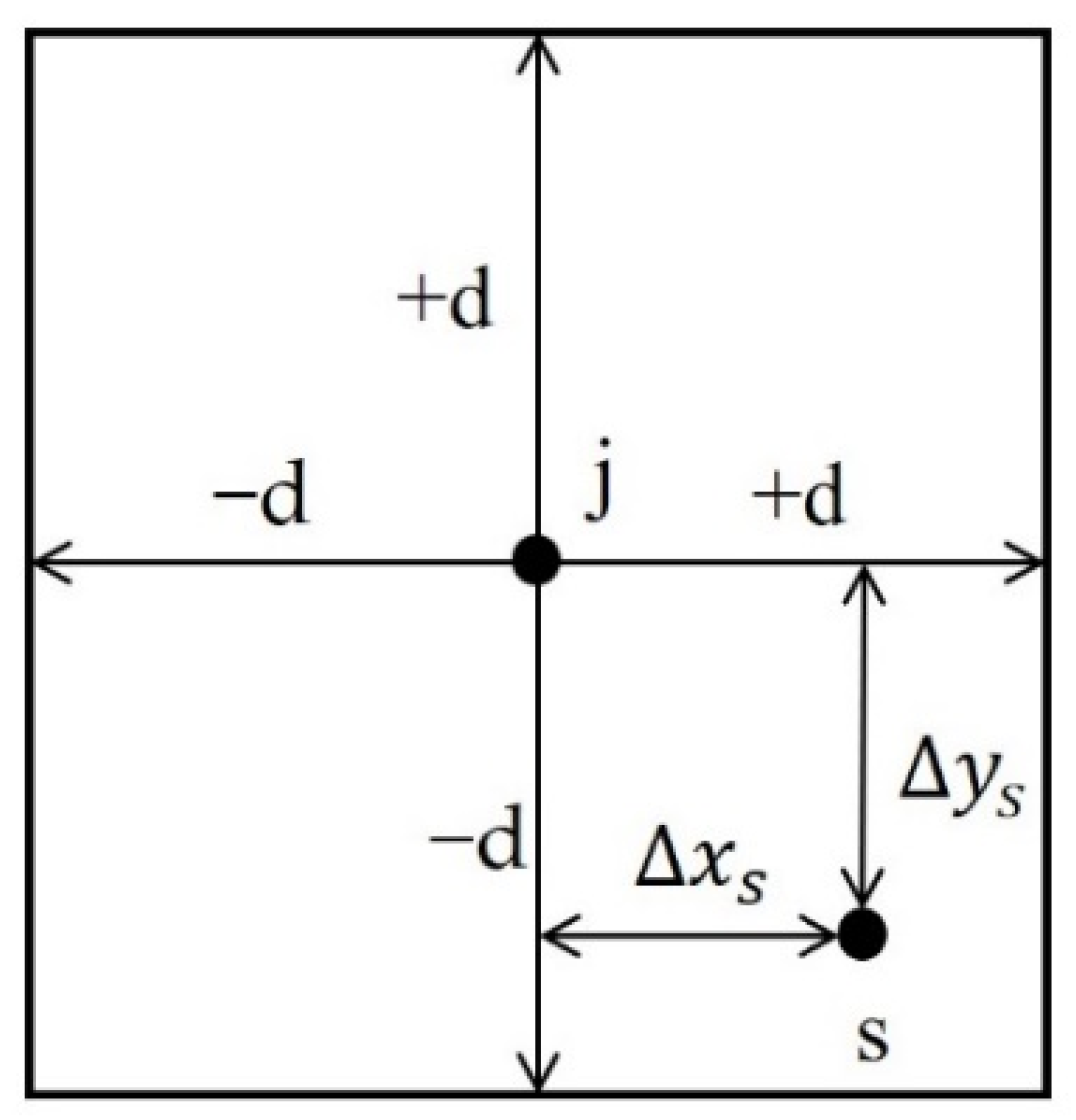
Based on the address of each manufacturing factory in China derived from the Chinese Industrial Enterprises Database, the address resolution method was used to determine the latitude and longitude of each factory. Next, based on the latitude and longitude data of the manufacturing factories, a factory scatter index (FSI) was calculated to measure the extent of the manufacturing factories’ dispersion [20]. The specific calculation method of the FSI is explained as follows: First, as shown in Figure 1, using the geographic location information of each manufacturing enterprise, we took a certain enterprise j as the center and created 4 square grids with side length d around it.

The average distance between one factory and all the factories in surrounding grids is calculated as follows.

$$d_j=\frac{{{\displaystyle \sum }}_{s=1}^{m_j}\sqrt{\Delta x_s^2+\Delta y_s^2}}{m_j}$$

(1)

where $d_j$ is the average distance, j is a factory, $\Delta x_s$ is the distance from factory s to factory j on the latitude, $\Delta y_s$ is the distance on the longitude, and $m_j$ represents the number of factories around factory j that meet the following conditions: $j\in i$ and −6 km ≤ $\Delta x_j$, $\Delta y_j$ ≤ +6 km [20,21].

Next, the FSI value of a research unit is the average $d_j$ of all enterprises in the region:

$$D_i=\frac{{{\displaystyle \sum }}_{j=1}^{t_i}{d}_j}{t_i}$$

(2)

where $D_i$ is the average $d_j$, i.e., FSI, i represents a study unit, and $t_i$ is the number of factories in study unit i.

2.2. Models and Variables

We used the following three models to study the influencing factors of groundwater withdrawal. The first model was ordinary least squares (OLS), which uses all variables to fit a single linear regression. Its expression formula is:

$$ln{y}_i={\beta }_0+{\displaystyle \sum }{\beta }_i{x}_i+{\epsilon }_i$$

(3)

where $ln{y}_i$ is the dependent variable, $x_i$. is the independent variables, ${\beta }_0$ is a constant term, ${\beta }_{\mathrm{i}}$ is the coefficient of the explanatory variables, and ${\epsilon }_i$ is the random error.

It was found that there were areas where groundwater withdrawal was 0 (about 11.2% of all samples). Thus, the Tobit model was used to eliminate the influence of the 0 value. Its expression formula is the same as that of the OLS regression.

To further examine the relationship between independent variables and the dependent variable with consideration of their spatial variations, the geographically weighted regression (GWR) model was also used to integrate the geographic coordinates of each observation into the linear regression model. The expression formula of the GWR model is:

$$ln{y}_i={\beta }_0{}_{\left(u_i,v_i\right) }+{\displaystyle \sum }{\beta }_k{}_{\left(u_i,v_i\right)}{x}_{ik}+{\epsilon }_i$$

(4)

where $ln{y}_i$ is the dependent variable, ${\beta }_0$ is a constant term, $\left(u_i,v_i\right)$ is the spatial position of the sampling point i, ${\beta }_k{}_{\left(u_i,v_i\right)}$ is the correlation coefficient between variables at point $\left(u_i,v_i\right)$, $x_{ik}$ is the independent variable, and ${\epsilon }_i$ is the random error.

In all models, the logarithm of groundwater withdrawal was taken as the dependent variable. Since groundwater withdrawal data at the district and county level was not available, we took 205 provincial-level secondary river basins in China as samples.

We also calculated the FSI value of each basin as our key independent variable. Based on related literature, we considered both natural and social–economic factors as independent variables to examine their influence on groundwater withdrawal.

• Social-economic factors

In China, the main types of water use are agricultural water, industrial water, and residential water. Among them, agriculture is the largest user of groundwater in China [22]. Because the amount of water used in agriculture is closely related to the area irrigated, it is characterized by the area of actual irrigated land. According to the results of a national water conservancy census in 2011, in that year, high-water consumption industries accounted for 3/4 of China’s total industrial water consumption. Therefore, we used the number of high-water consumption plants and the proportion of high-water consumption plants to the total number of factories to represent industrial water usage. Residential water use is closely related to population size and level of urbanization, so we adopted the total population and urbanization rate. At the same time, economic efficiency and water use efficiency can also affect water consumption, so we chose Gross Domestic Product (GDP) per capita and water withdrawal per GDP as indicators.

• Natural factors

For natural factors, we used the average rainfall per year to control for the impact of surface water changes on water consumption and added annual average temperature to express the possible impact of temperature changes on water demand.

Moreover, considering the differences in factors such as hydrology and climate between North China and South China, provinces were divided into northern provinces and southern provinces according to the perspective of economic geography of Sheng et al. (2018) [23]. Precisely, Beijing, Tianjin, Hebei, Shanxi, Shaanxi, Heilongjiang, Jilin, Liaoning, Inner Mongolia, Ningxia, Gansu, Xinjiang, and Qinghai were included in the northern region, and the remaining 18 provinces and cities (excluding Hong Kong, Macao, and Taiwan) were included in the southern region. Based on that, a dummy variable was constructed, namely whether the provincial-level secondary river basin was in South China.

Groundwater withdrawal data, agricultural irrigation data, water use efficiency data and annual average rainfall data were all collected from the Chinese Water Resources Bulletin (2016) and were assigned to provincial-level secondary river basins based on certain rules. Factory locations and the number and proportion of high-water consumption factories were all retrieved from the Chinese Industrial Enterprise Database. Because the Chinese Industrial Enterprise Database stopped updating in 2013, we used the latest 2013 enterprise data. For population and urbanization data, we believe that census data is more comprehensive and accurate than sample data. Therefore, we collected them from the latest China Population Census in 2010. Data on GDP per capita was taken from China’s County and City Economic Statistics Yearbook for 2016. The annual average temperature data was acquired from the Climatic Research Unit Global Climate Dataset (version 4.03).

Table 1. Variable Summary Statistics.

Variable		Observations	Mean	SD	Min	Max
Dependent variable	Groundwater withdrawal (104 m3)	205	5.1560	11.848	0.000	89.220
Social–economic factors	Factory scatter index (FSI) (km)	179	2.2330	1.165	0.000	5.065
	Area of actual irrigated land (104 m2)	205	425.6320	832.676	0.000	6840.100
	Number of high-water consumption plants	175	526.4630	1080.326	1.000	6457.000
	Proportion of high-water consumption plants (%) 1	175	30.7850	17.000	0.000	100.000
	Total population (×104)	205	673.7730	1078.268	0.000	6663.180
	Urbanization rate (%)	190	44.1540	20.668	0.000	95.667
	GDP per capita (104 yuan/person)	190	4.4080	2.985	0.000	17.387
	Water withdrawal per GDP (yuan/m3)	181	0.0129	0.016	0.001	0.123
Natural factors	Rainfall (mm)	204	815.7960	555.906	0.000	2540.349
	Temperature (°C)	204	8.9610	8.023	−20.494	22.798

¹ We used the factories above the designated size in China in the thermal power industry and other high-water consumption industries as high-water consumption factories. Among them, industrial enterprises above a designated size in China refer to the enterprises whose annual revenue of main business is more than 20 million yuan according to the National Bureau of Statistics of China.

shows the summary statistics for all variables. Due to the differences in the units of each variable, we normalized all the original data.

Table A1. Correlation matrix between the independent variables after normalization.

	FSI	Number of High-Water Consumption Plants	Total Population	Area of Actual Irrigated Land	Proportion of High-Water Consumption Plants	Proportion of High-Water Consumption Plants	GDP per Capita	Water Withdrawal per GDP	Rainfall	Temperature
FSI	1
Number of high-water consumption plants	0.3959	1
Total population	0.3575	0.7042	1
Area of irrigated land	0.1643	0.4513	0.7561	1
Proportion of high-water consumption plants	−0.2284	−0.0838	−0.0618	0.0061	1
Proportion of high-water consumption plants	0.4653	0.3629	0.3846	0.2129	−0.2442	1
GDP per capita	0.432	0.4192	0.3261	0.144	−0.0919	0.68	1
Water withdrawal per GDP	−0.2001	−0.209	−0.2066	−0.0636	0.1351	−0.3529	−0.2687	1
Rainfall	0.3312	0.2605	0.2629	0.1477	−0.0783	0.1646	0.2404	0.1175	1
Temperature	0.2712	0.2447	0.2215	0.1446	−0.0361	0.1249	0.2182	0.1836	0.8014	1

reports the correlation coefficients between the independent variables (after normalization). Although there was a high correlation between temperature and rainfall, they did not affect the target variable. Additionally, the calculated variance inflation factor was less than 5. Therefore, there was no serious multicollinearity existing among independent variables.

3. Results

3.1. General Characteristics of the Distribution of Manufacturing Plants in China

In this section, we calculate the number of manufacturing plants and FSIs in the four geographic regions of East China, Central China, West China, and Northeast China, respectively, and subdivide areas in the four regions into districts and counties—which were classified based on the administrative division of China in 2015—in order to compare the differences between urban and non-urban areas.

As shown in

Table 2. The number of manufacturing plants in different regions of China.

	Total
Region	East China	Central China	West China	Northeast China	China
Number of manufacturing plants in 2000	93,972	30,924	23,033	11,356	159,285
Number of manufacturing plants in 2010	303,540	83,690	46,127	23,395	456,752
Change rate (2000–2010) (%)	223.01	170.63	100.26	106.01	186.75
	Counties
Region	East China	Central China	West China	Northeast China	China
Number of manufacturing plants in 2000	37,769	20,226	12,196	4525	74,716
Number of manufacturing plants in 2010	143,361	58,221	24,345	10,318	236,245
Change rate (2000–2010) (%)	279.57	187.85	99.61	128.02	216.19
	Districts
Region	East China	Central China	West China	Northeast China	China
Number of manufacturing plants in 2000	56,203	10,698	10,837	6831	84,569
Number of manufacturing plants in 2010	160,179	25,469	21,782	13,077	220,507
Change rate (2000–2010) (%)	185.00	138.07	101.00	91.44	160.74

, from 2000 to 2010, the number of manufacturing plants in China increased by nearly two times. Among the four regions, East China had the largest number of manufacturing plants and the fastest growth rate of 223%. From the comparison of counties and districts, in East China and North China, the number of manufacturing plants in districts was found to be more than that in counties in both 2000 and 2010; meanwhile, in Central China and West China, the number of manufacturing plants in districts was always less than that in counties. Additionally, in East, Central, and Northeast China, the growth rate of the number of manufacturing plants in counties was higher than that in districts.

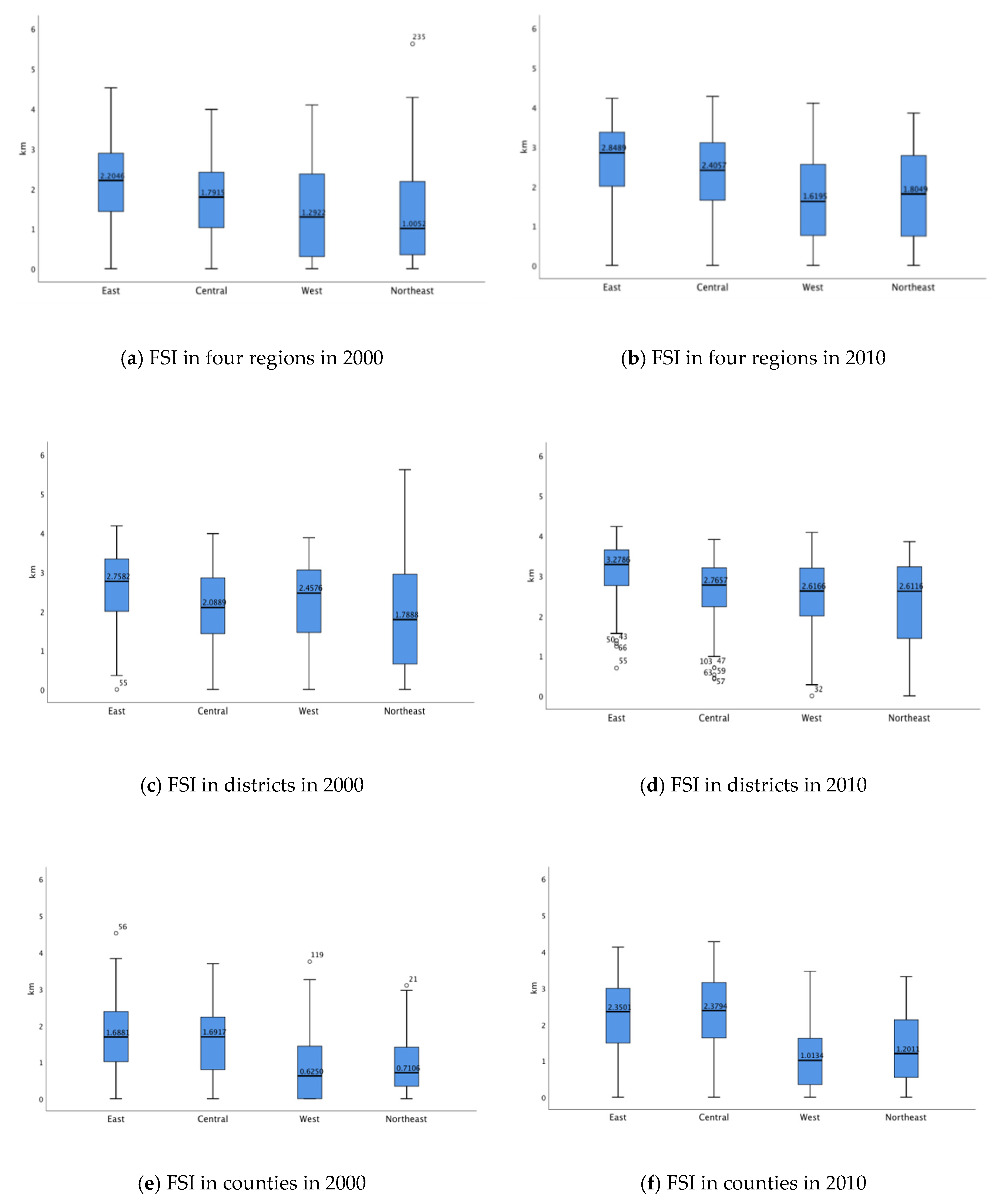
Figure 2 displays the FSIs in different regions of China in 2000 and 2010 and further shows the FSIs by district and county. As can be seen from Figure 2, in each region, the FSIs increased from 2000 to 2010. Among them, the FSIs in East China and Central China had relatively higher average values and shorter box lengths, which indicated that the FSIs in these two regions were concentrated at higher average values. In other words, the distribution of manufacturing plants was more scattered in these two regions than in other regions. In terms of districts and counties, it can be seen that in 2000 and 2010, the FSIs in districts were higher than those in counties, and the average FSIs in districts in different regions of China were similar. Additionally, from 2000 to 2010, the average FSIs in counties increased more than those in districts.

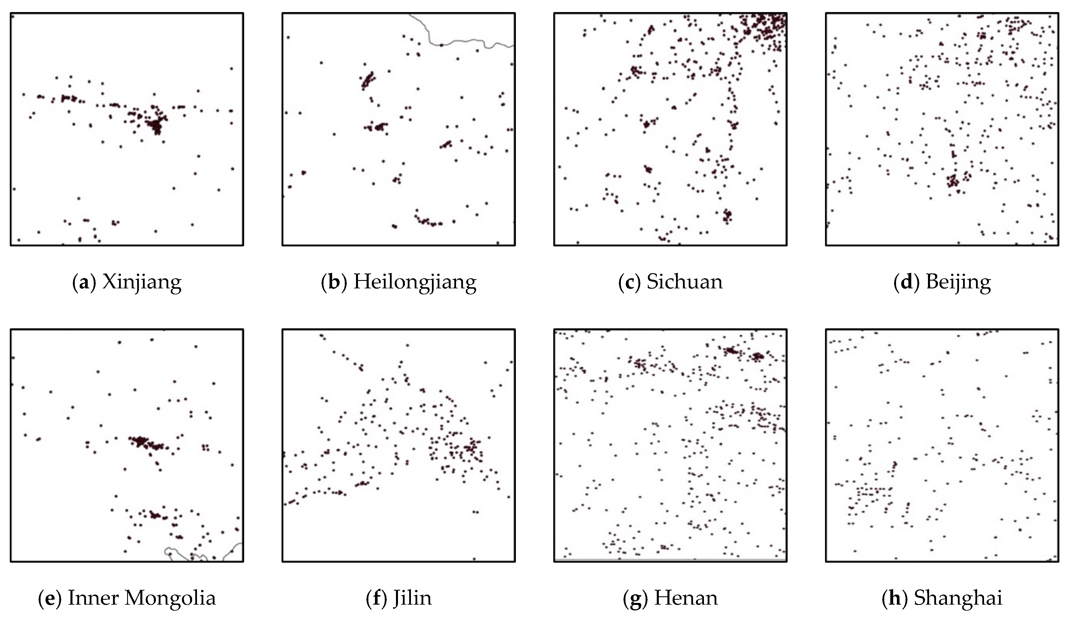
Finally, in order to present the distribution of manufacturing plants in different regions of China with different FSIs more intuitively, we calculated the FSIs by province and displayed the distribution of manufacturing plants in the four provinces with the highest FSIs in 2000 and 2010, respectively, as shown in Figure A1.

3.2. The Evolution of the Spatial Distribution of Manufacturing Plants in China

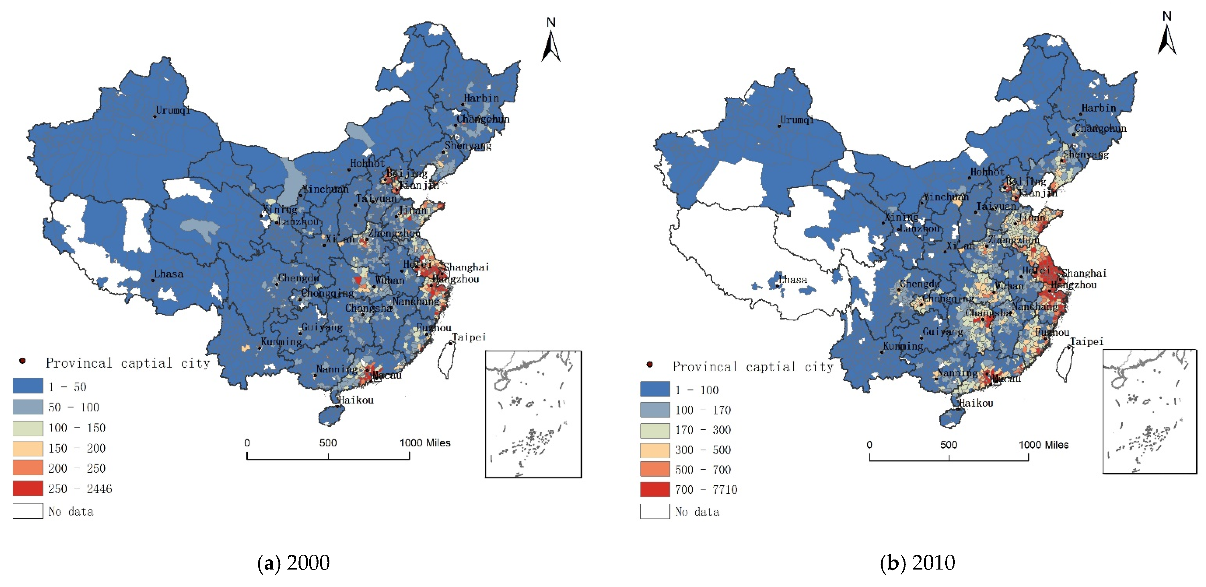
Figure A2 shows the number of manufacturing plants in districts and counties of China in 2000 and 2010. It was found that between 2000 and 2010, the manufacturing industry began to shift to Central and West China while continuing to develop in East China. Specifically, in 2000, a large number of manufacturing plants were concentrated in the Yangtze River Delta, Pearl River Delta, Shandong Peninsula, and other eastern coastal areas (see Figure A2a); meanwhile, by 2010, the number of manufacturing plants in the coastal areas of East China had increased significantly, and some areas in Central and West China such as eastern Hunan, eastern Hubei, Chengdu, and Chongqing had also seen an intense growth in the number of manufacturing plants (see Figure A2b).

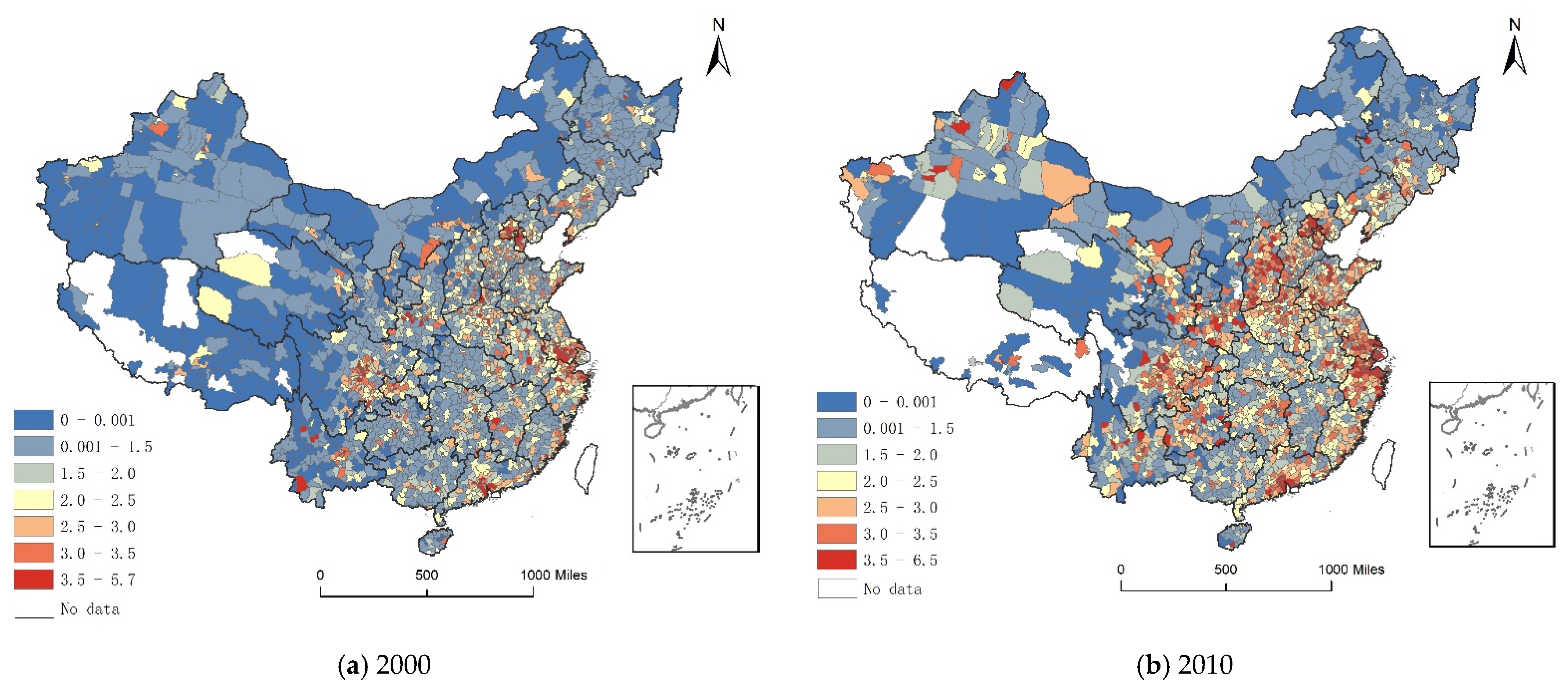
Figure 3 displays the values of the FSIs in districts and counties of China in 2000 and 2010. It was found that the scattering of manufacturing plants was relatively high in China, and that the value of FSIs increased from 2000 to 2010, with the degree of scattering being highest in 2010.

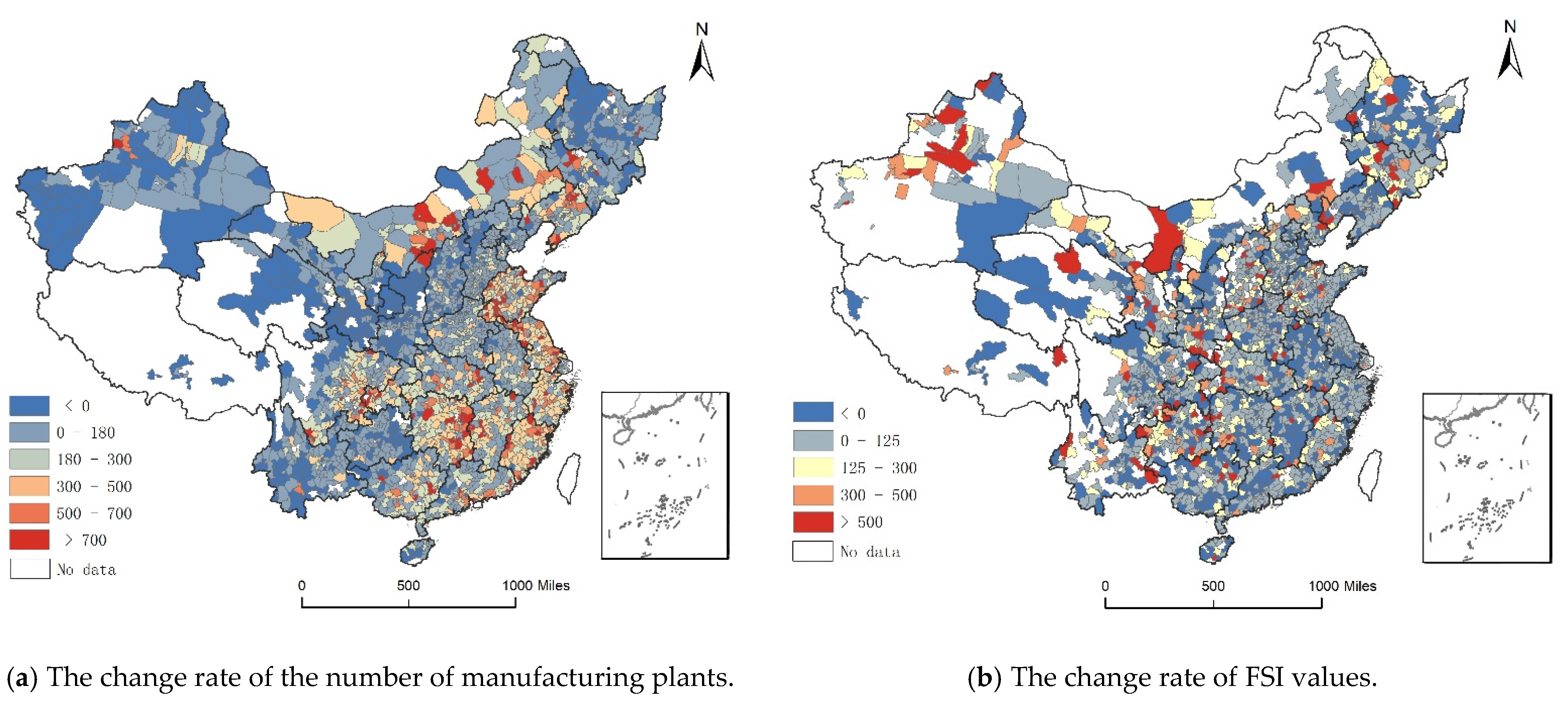
Figure 4 displays the change rate of the number of manufacturing plants and FSIs from 2000 to 2010 in districts and counties of China. It can be seen that the counties or districts with the largest increase in the number of plants were not necessarily those with the largest increase in FSIs. For example, the Jiangsu and Zhejiang Provinces in East China and Jiangxi Province in Central China all had relatively large growth rates of the number of manufacturing plants and relatively lower rates of change of FSIs. Among them, the FSIs of most districts and counties in Jiangxi Province showed a negative growth trend. Additionally, a very prominent feature was that the districts and counties with the largest growth rates of FSIs appeared at the boundary between adjacent provinces.

In order to more clearly compare the degree of scattering of manufacturing plants in various regions, we calculated the change rate of FSIs and the number of manufacturing plants and its change rate in each province of China (

Table 3. The change rate of the number of manufacturing plants and the change rate of FSIs in different provinces from 2000 to 2010.

Province 1	Manufacturing Plants in 2000	Rank	Manufacturing Plants in 2010	Rank	Change Rate of the Number of Manufacturing Plants (%)	Rank	Change Rate of FSIs (%)	Rank
National average	5887	11	17,293	9	147	13	33	12
Jiangsu	16,201	2	74,809	1	361.76	2	9.65	26
Zhengjiang	14,720	3	62,084	3	321.77	3	13.05	25
Beijing	4803	13	6404	18	33.33	22	14.3	24
Fujiang	6010	8	24,533	5	308.2	4	17.88	22
Guangdong	18,697	1	64,486	2	244.9	6	25.8	15
Hebei	7282	7	10,806	14	48.39	19	27.38	14
Shanghai	8771	6	15,102	11	72.18	18	37.51	11
Hainan	505	26	906	26	79.41	17	43.1	8
Tianjing	5313	12	6348	19	19.48	25	46.12	7
Shandong	11,670	4	38,062	4	226.15	8	58.79	3
Jiangxi	3598	17	12,077	13	235.66	7	9.17	27
Anhui	3685	16	8034	16	118.02	14	18.31	21
Henan	9856	5	19,588	7	98.74	15	24.08	17
Hunan	4687	14	21,896	6	367.16	1	37.84	10
Hubei	5919	10	17,618	8	197.65	10	41.66	9
Shanxi	3179	19	4477	20	40.83	21	65.51	2
Chongqing	1955	25	7974	17	307.88	5	17.88	23
Shanxi	2665	22	3366	22	26.3	23	18.38	20
Sichuan	4411	15	13,281	12	201.09	9	23.33	19
Guanxi	3246	18	8690	15	167.71	12	24.62	16
Ningxia	407	27	736	27	80.84	16	29.74	13
Guizhou	1984	24	2240	25	12.9	27	52.61	5
Yunan	2154	23	2694	24	25.07	24	54.96	4
Liaoning	5925	9	16,413	10	177.01	11	23.68	18
Heilongjian	2695	21	3045	23	12.99	26	46.61	6
Jilin	2736	20	3937	21	43.9	20	88.73	1

¹ Due to the incompleteness of the information about the plants in districts and counties of the provinces of Xinjiang, Tibet, Inner Mongolia, Gansu, and Qinghai, these areas are not discussed.

). As shown in Table 3, the national average change rate of FSIs from 2000 to 2010 was 33%. Among the 26 studied provinces, 11 had FSI change rates that were higher than the national average. By comparing the change rate of the number of manufacturing plants and the change rate of FSIs, it was found that the provinces with the largest increase in the number of manufacturing plants were not necessarily those with the largest change rate of FSIs. In other words, the increase in the number of manufacturing plants did not necessarily lead to the spatial scattering of manufacturing plants, which was consistent with the above conclusion.

3.3. Empirical Results

In this section, OLS regression, Tobit regression, and GWR are carried out in turn to examine the relationship between the degree of scattering of manufacturing plants and groundwater withdrawal.

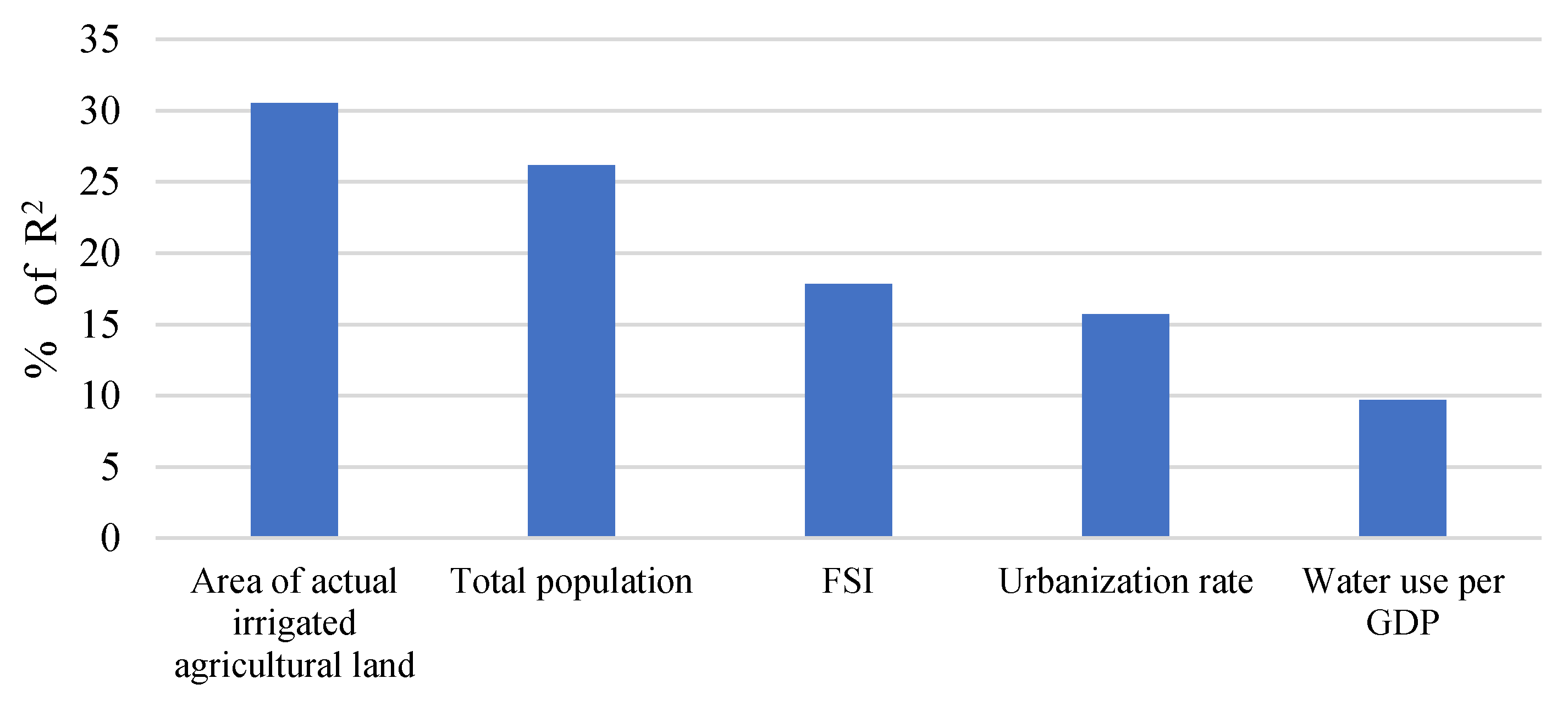
As shown in

Table 4. The results of ordinary least squares (OLS) regression and Tobit regression.

	(1)	(2)	(3)	(4)	(5)	(6)	(7)	(8)
Variable	OLS 1	OLS 2	OLS 3	OLS 4	Tobit 1	Tobit 2	Tobit 3	Tobit 4
FSI	0.471 ***	0.168 **	0.235 **	0.233 **	0.455 ***	0.179 *	0.236 ***	0.234 ***
	(0.078)	(0.0848)	(0.0903)	(0.0904)	(0.0723)	(0.0721)	(0.0764)	(0.0764)
Area of actual irrigated land		0.643 **	0.586 *	0.582 *		0.642 ***	0.573 ***	0.570 ***
		(0.32)	(0.302)	(0.311)		(0.143)	(0.145)	(0.146)
Number of high-water consumption plants		−0.122	−0.123	−0.123		−0.125	−0.121	−0.12
		(0.11)	(0.123)	(0.126)		(0.104)	(0.107)	(0.107)
Proportion of high-water consumption plants		−0.0987	−0.131	−0.14		−0.0864	−0.117	−0.124
		(0.109)	(0.12)	(0.128)		(0.0882)	(0.094)	(0.0951)
Total population		0.318	0.381 *	0.384 *		0.296 **	0.364 **	0.366 **
		(0.202)	(0.207)	(0.208)		(0.14)	(0.141)	(0.141)
Urbanization rate		0.250 ***	0.212 **	0.208 **		0.213 ***	0.184 **	0.181 *
		(0.0852)	(0.0933)	(0.0933)		(0.0741)	(0.0912)	(0.0918)
GDP per capita			0.0207	0.0206			0.00793	0.00715
			(0.0935)	(0.0962)			(0.0999)	(0.1)
Water withdrawal per GDP			0.321 *	0.317 *			0.357 **	0.352 **
			(0.174)	(0.175)			(0.167)	(0.17)
Rainfall				−0.0749				−0.0517
				(0.15)				(0.111)
Temperature				0.0679				0.0518
				(0.127)				(0.113)
Dummy	0.179 ***	0.160 ***	0.174 ***	0.168 ***	0.174 ***	0.150 ***	0.163 ***	0.159 ***
	(0.032)	(0.027)	(0.0276)	(0.0394)	(0.0335)	(0.027)	(0.0274)	(0.0356)
Intercept	0.260 ***	0.254 ***	0.208 ***	0.196 *	0.276 ***	0.278 ***	0.233 ***	0.221 ***
	(0.0408)	(0.0655)	(0.0793)	(0.104)	(0.0419)	(0.0556)	(0.0645)	(0.084)
N	182	160	153	153	182	160	153	153
R2	0.229	0.52	0.521	0.522

Note: Standard errors are in parentheses; * p < 0.1, ** p < 0.05, *** p < 0.01.

, of all the OLS regression results, column (4) performed best, explaining 52.2% of the groundwater withdrawal. Among them, the FSI showed a relatively high importance in the model, accounting for 17.85% of the groundwater withdrawal and ranking third among all the influencing factors (see Figure A3). Generally, the coefficients of the FSI in all models were significantly positive, indicating that the dispersed distribution of manufacturing plants had a significant influence on groundwater withdrawal. Additionally, the coefficient values of the two variables, the total population, and the area of actual irrigated land were also significantly positive in all the models, which was consistent with reality. Furthermore, the urbanization rate was found to be significantly positively correlated with groundwater withdrawal, meaning that the increase in the urbanization rate would aggravate groundwater withdrawal. Finally, there was a positive relationship between groundwater consumption and water withdrawal per GDP, which indicated that the lower the water withdrawal efficiency, the more groundwater was used.

Furthermore, the regression results of the Tobit model were basically consistent with those of the OLS model (see Table 4, column (5)–(8)); therefore, no further explanation of the results of this model were given.

Table 5. The results of geographically weighted regression (GWR).

Variable	Min	Q(1/4)	Q(1/2)	Q(3/4)	Max
FSI	0.104	0.133	0.177	0.218	0.378
Area of irrigated land	0.264	1.088	1.281	1.391	1.532
Number of high-water consumption plants	−0.354	−0.218	−0.178	−0.137	0.097
Proportion of high-water consumption plants	−0.287	−0.247	−0.181	−0.046	0.137
Total population	−0.160	−0.070	−0.004	0.057	0.453
Urbanization rate	0.130	0.187	0.228	0.334	0.597
GDP per capita	−0.143	−0.019	0.065	0.127	0.193
Water withdrawal per GDP	−0.781	−0.585	−0.432	−0.020	0.490
Rainfall	−0.988	−0.398	−0.284	−0.115	0.098
Temperature	−0.307	−0.126	−0.012	0.059	0.611
Intercept	0.089	0.346	0.451	0.539	0.632

shows the results of the GWR. The coefficient of FSI was stable to positive in all results of the GWR with a minimum value of 0.1043 and a maximum value of 0.3782, confirming that the more scattered the spatial distribution of manufacturing plants, the greater the groundwater withdrawal.

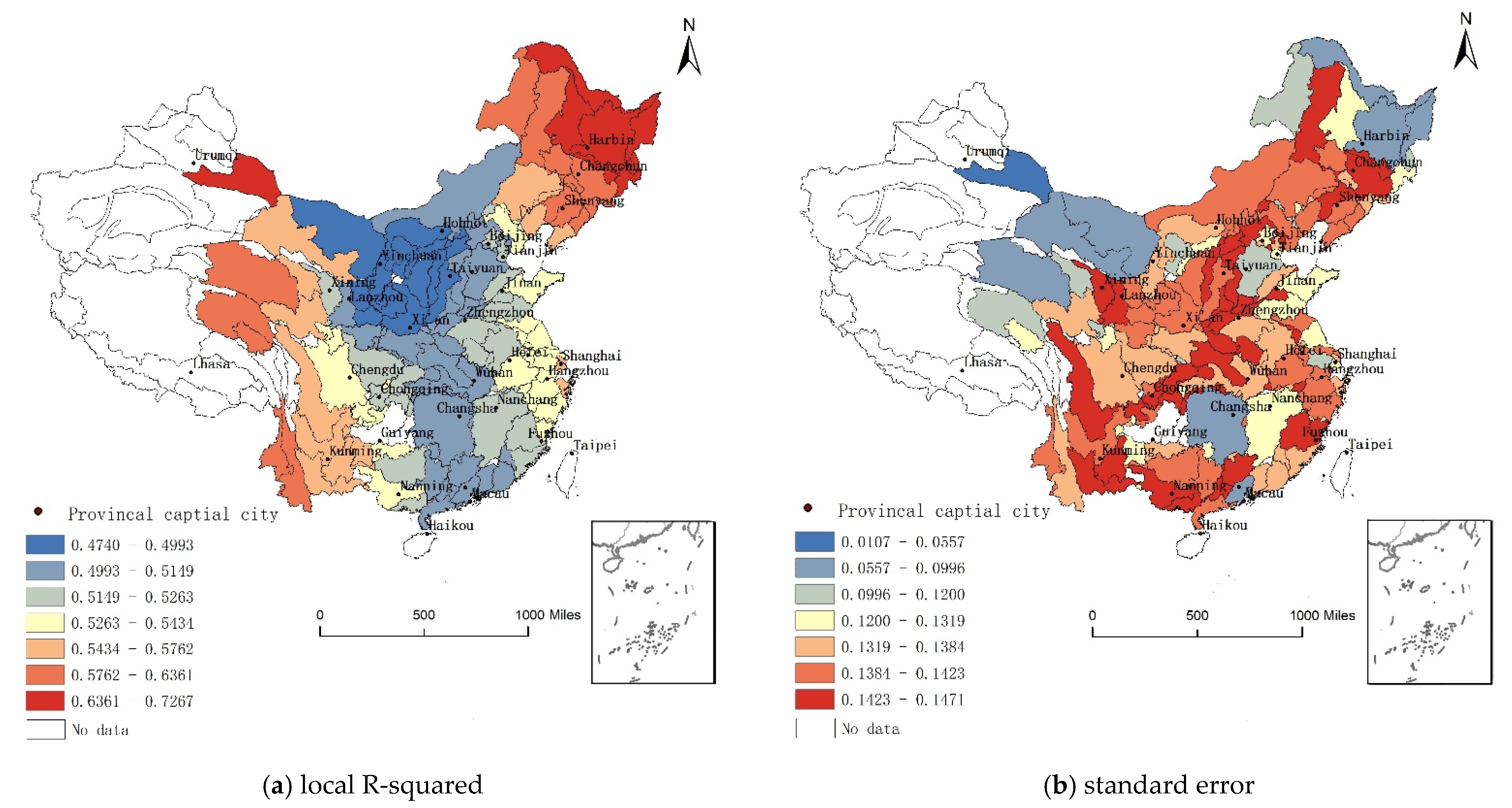
In

Table A2. A comparison of the regression results of the OLS and GWR models.

Model	AIC 1	R2	Adjusted R2
OLS	−94.49802	0.5222	0.4849
GWR	−119.56729	0.6829	0.6045

¹ AIC: Akaike information criterion.

, we compare some of the statistics of the OLS model with those of the GWR model. It can be seen that compared with the OLS model, GWR has a lower Akaike information criterion (AIC) value and a higher R-squared value. Therefore, GWR performed better than OLS. The GWR model explained 60% of the variation in groundwater withdrawal. The important improvement in the performance of the GWR relative to the OLS regression indicated that our spatial data had the characteristics of spatial non-stationarity. Therefore, we further analyzed the spatial differences of the R-squared values, standard errors, and coefficient values of the GWR model. As shown in Figure A4, local R-squared values varied from 0.474 to 0.7267 (Figure A4a), and the standard errors varied from 0.0107 to 0.1471 (Figure A4b). In addition, the GWR coefficients varied significantly between different regions of China. Specifically, the coefficients of the FSI were relatively small in Hebei, Tianjin, Beijing, and Inner Mongolia, while large in West China, which is the most ecologically fragile.

4. Discussion

4.1. Regional Differences in the Degree of Scattering of Manufacturing Plants

In our analysis, we found that FSI values in districts were higher than those in counties, and the average FSIs in districts in different regions of China were similar, suggesting that factories within a district are generally farther apart from each other. High land rents owing to high levels of urban services and infrastructure in the districts often push manufacturing to the fringes where the distances between manufacturing plants are often far apart.

Additionally, from 2000 to 2010, the average FSIs in counties increased more than those in districts. Therefore, recently, it was the counties, with relatively low land prices and weak environmental management regulations, that had taken over most of the manufacturing plants. In China, counties usually have fierce competition in attracting investment. Therefore, local governments, especially those in less developed areas, are more supportive than regulatory to manufacturing plants. For example, when Foxconn moved to Jincheng, Shanxi Province, the local government provided the most favorable policies for land, labor recruitment, water and electricity supply, and tax breaks [24]. As a result, the lack of planning in site selection often leads to a spatially dispersed distribution of regional manufacturing [25].

Some researchers may argue that an increase in the distance between plants (i.e., FSI value) is inevitable, especially when a large number of manufacturing plants enter along with rapid industrial development. However, our results found that the districts or counties with the largest increase in the number of manufacturing plants were not necessarily those with the largest increase in FSI values. In Jiangsu Province, the number of manufacturing plants increased greatly between 2000 and 2010, but the growth rate of the FSI during this period was small, which meant that the average distance between factories did not increase much. It seems that the spatial pattern of plants can be adjusted by local governments’ planning and management [26]. The FSI index can reflect the extent to which local governments’ planning and management play a role in formatting an appropriate spatial structure.

Interestingly, districts or counties with the largest increase in the scattering degree of manufacturing plants appeared at the boundary between neighboring provinces. Plants located there can often easily escape punishment for polluting because their emissions often affect neighboring provinces. Disputes over pollution need to be reported to higher-level government, which makes management more difficult. Therefore, people there often choose to close an eye to them, and local governments tend to implement loose land planning and management in border areas [27]. Therefore, the plants there are often located according to their own requirements, e.g., large areas of single-story plants, which leads to a dispersed distribution of manufacturing plants there.

4.2. Effects of the Scattering of Manufacturing Plants on Groundwater Withdrawal

The results of this study suggest that the dispersed distribution of manufacturing plants has a significant impact on groundwater withdrawal, accounting for 17.85% of the dependent variable in the model; that is, the more scattered the manufacturing plants, the larger the groundwater withdrawal. In China, areas of enterprise clusters (such as industrial parks) are usually equipped with complete municipal waterworks and facilities [28]. Therefore, it is convenient to monitor and charge for the water consumption of manufacturing plants, and it is also easier for local water resources departments to supervise water use in the cluster areas. Since strict management can lead to an increase in costs, manufacturing plants have to reduce their costs by improving resource utilization efficiency such as by saving water or upgrading technology [29]. Therefore, the manufacturing plants in the cluster areas tend to reduce the use of groundwater.

However, scattered distribution of manufacturing plants increases the cost of pipeline laying, making municipal works difficult. In addition, due to advances in water drilling technology, scattered factories usually have chosen to drill on-site, especially when China did not restrict well drilling in previous years (e.g., in 2011, 58 counties in Hebei province drilled more than 10,000 wells, including 6 counties that drilled more than 100,000 wells) [20]. Manufacturers scattered across rural areas may also share wells with villagers. In such cases, the amount of water used by factories cannot be assessed quantitatively, and strict monitoring cannot be performed [30]. The cost of water for scattered factories is relatively low; factories that share wells with villagers usually pay only a small fee to the local village. Therefore, with convenient well drilling and low water costs, manufacturing plants have weak awareness of water conservation, and groundwater over-extraction and waste occur frequently.

Moreover, in the absence of environmental regulation, scattered manufacturing plants, especially polluting ones, usually discharge more heavily [31,32]. The discharge of sewage into local rivers leads to surface water contamination, leaving no available clean surface water, which in turn causes the entire region to rely on groundwater [33]. The discharge of wastewater has an important indirect but non-negligible impact on the increase of groundwater use throughout China.

It is clear that the scattering of manufacturing plants and the corresponding water management play an exceptionally significant role in groundwater withdrawal that deserves much attention.

4.3. Regional Differences in the Effects of the Scattering of Manufacturing Plants on Groundwater Withdrawal

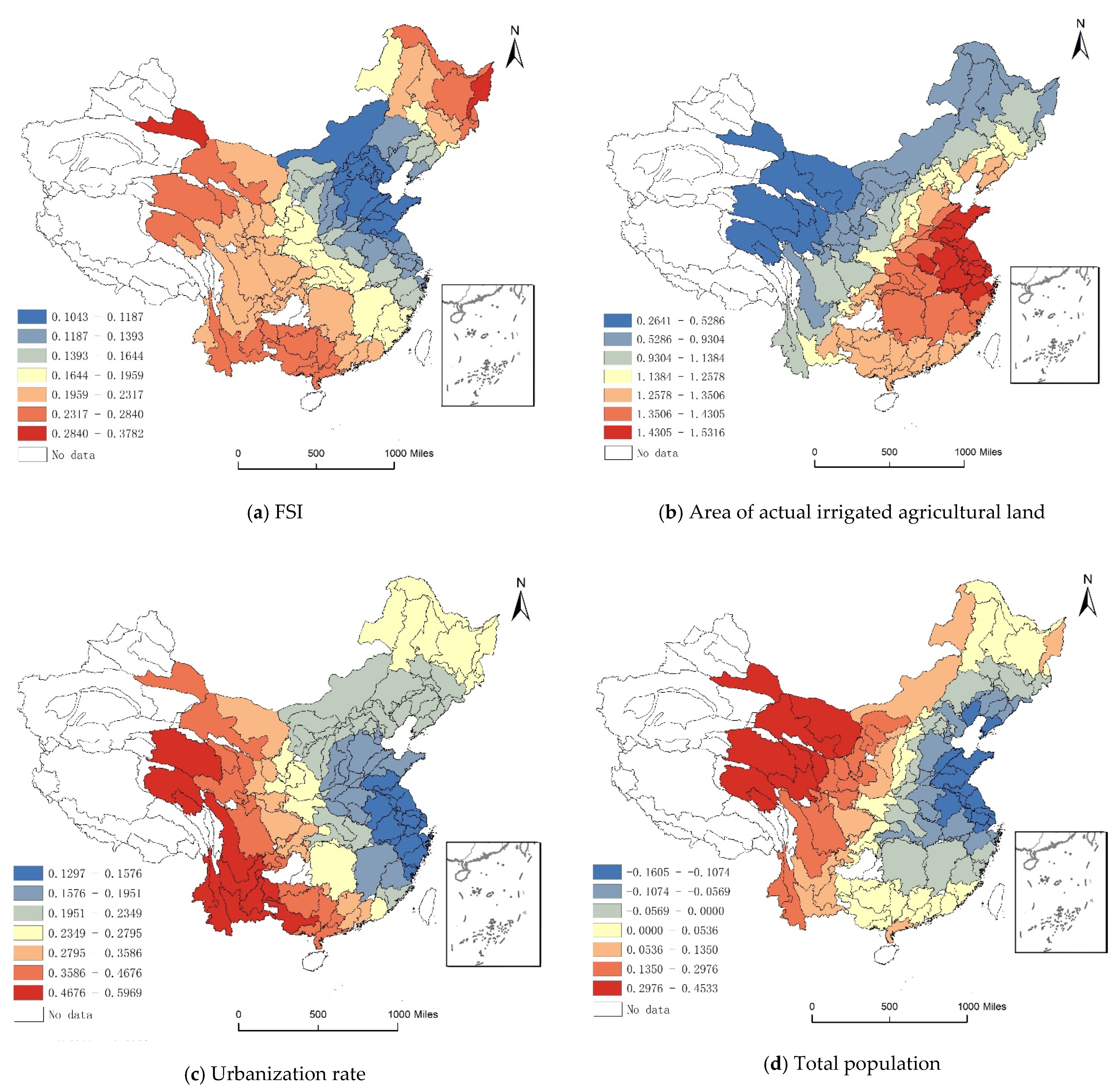
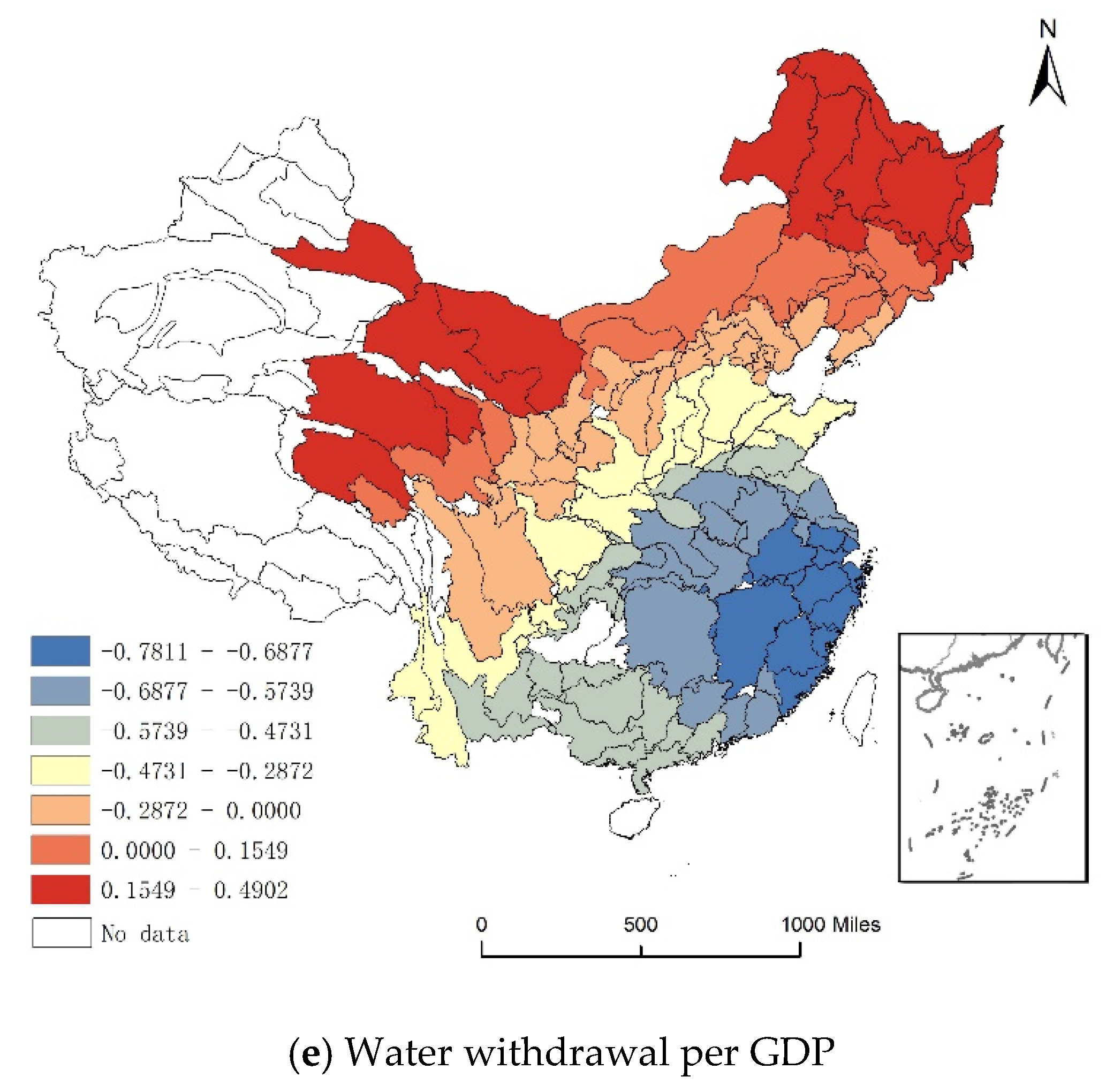
The regression results of the GWR model (Figure 5) show that the impact of the degree of scattering of manufacturing plants on groundwater withdrawal varies in different regions of China. As such, when planning efficient water resource development, it may be more useful to adopt different water conservation strategies in different regions according to spatially varying trends in groundwater withdrawal than to adopt a “one size fits all” strategy.

It is noted that the spatial scattering of manufacturing plants is not the most important factor affecting groundwater withdrawal in North China (Figure 5a). The actual irrigated agricultural area is the main variable affecting groundwater consumption there (Figure 5b). This is consistent with the results of Tian et al. (2016), who found that agricultural irrigation was the main factor affecting groundwater withdrawal in the North China Plain, and the greater the dependence of agricultural irrigation water on groundwater, the more serious the groundwater withdrawal [34].

However, the spatial scattering of manufacturing plants has a great impact on groundwater withdrawal in West China, especially in areas with a fragile ecological-environment (Figure 5a). The reasons for this are as follows: First of all, groundwater is an important source for industrial, agricultural, and domestic usage in West China due to a severe shortage of available surface water [35]. Secondly, compared with East China, West China is geographically vast and sparsely populated, so the cost of tap water transmission caused by the scattered distribution of manufacturing plants is much higher. Additionally, the broad jurisdiction of district and county governments in West China makes it more difficult to regulate the use of water by scattered manufacturing plants. Therefore, in West China, factories often choose to use groundwater, which is more convenient and available, to save costs. Thirdly, due to the lack of unified water withdrawal planning in West China, the structure of water use and industry is irrational, resulting in the low efficiency of water withdrawal [36]. The ecological environment of West China is extremely fragile, and groundwater withdrawal aggravates this vulnerability, thus affecting local sustainable development [37,38].

5. Conclusions

Our empirical research highlights the importance of introducing the distribution of manufacturing plants into the groundwater use analysis framework. We found that the scattered distribution of manufacturing plants played a key role in groundwater withdrawal in China, especially in areas with a fragile ecological environment. The scattered distribution of manufacturing plants raises the cost of tap water transmission, makes monitoring and supervision more difficult, and increases the possibility of surface water pollution, thereby intensifying groundwater withdrawal. This finding may serve as a basis for the reasonable adjustment of the spatial distribution of manufacturing factories to reduce groundwater withdrawal and realize the protection of groundwater, especially in areas with water shortages, a high dependence on groundwater, and fragile ecology. In this way, it can help effectively alleviate the pressure on the regional ecological environment.

At present, China is in the middle stage of industrialization, and the scattering of manufacturing plants is relatively high. Under increasingly severe resource and environmental constraints, exploring the relationship between the spatial pattern of manufacturing development and resource utilization is of great significance for solving problems related to resources and the environment. As seen in this paper, planning and management can play a very important role in the spatial distribution of manufacturing plants. Our conclusions provide an important practical geographical basis for the adjustment of the spatial distribution of manufacturing factories in areas with a fragile ecological environment and a severely scattered distribution of factories.

References

- De Graaf, I.E.M.; Gleeson, T.; Van Beek, L.P.H.; Sutanudjaja, E.H.; Bierkens, M.F.P. Environmental flow limits to global groundwater pumping. Nat. Cell Biol. 2019, 574, 90–94. [Google Scholar] [CrossRef]
- Braadbaart, O.; Braadbaart, F. Policing the urban pumping race: Industrial groundwater overexploitation in Indonesia. World Dev. 1997, 25, 199–210. [Google Scholar] [CrossRef]
- Koncagül, E. Facing the Challenges: Case Studies and Indicators: UNESCO’s Contributions to the United Nations World Water Development Report; UNESCO Publishing: Paris, France, 2015; Volume 2, pp. 4–5. [Google Scholar]
- Klingbeil, R.; Byiringiro, F. Food Security, Water Security, Improved Food Value Chains for a more Sustainable Socio-economic Development. In Sharaka Conference “eu-Gcc Regional Security Cooperation: Lessons Learned & Future Challenges”; CIDOB: Barcelona, Spain, 2013. [Google Scholar]
- Shah, T.; Molden, D.J.; Sakthivadivel, R.; Seckler, D. The Global Groundwater Situation: Overview of Opportunities and Challenges; International Water Management Institute (IWMI): Colombo, Sri Lanka, 2000. [Google Scholar]
- Hamdy, A.; Ragab, R.; Scarascia-Mugnozza, E. Coping with water scarcity: Water saving and increasing water productivity. Irrig. Drain. 2003, 52, 3–20. [Google Scholar] [CrossRef]
- Liu, Y.; Zhang, Z.; Zhang, F. Challenges for Water Security and Sustainable Socio-Economic Development: A Case Study of Industrial, Domestic Water Use and Pollution Management in Shandong, China. Water 2019, 11, 1630. [Google Scholar] [CrossRef] [Green Version]
- Yang, H.; Zhang, X.; Zehnder, A.J. Water scarcity, pricing mechanism and institutional reform in northern China irrigated agriculture. Agric. Water Manag. 2003, 61, 143–161. [Google Scholar] [CrossRef]
- Gilg, A.; Barr, S. Behavioural attitudes towards water saving? Evidence from a study of environmental actions. Ecol. Econ. 2006, 57, 400–414. [Google Scholar] [CrossRef]
- Chang, F.-J.; Huang, C.-W.; Cheng, S.-T.; Chang, L.-C. Conservation of groundwater from over-exploitation—Scientific analyses for groundwater resources management. Sci. Total Environ. 2017, 598, 828–838. [Google Scholar] [CrossRef] [PubMed]
- Gracia-De-Rentería, P.; Barberán, R.; Mur, J. The Groundwater Demand for Industrial Uses in Areas with Access to Drinking Publicly-Supplied Water: A Microdata Analysis. Water 2020, 12, 198. [Google Scholar] [CrossRef] [Green Version]
- Chang, H.; Parandvash, G.H.; Shandas, V. Spatial Variations of Single-Family Residential Water Consumption in Portland, Oregon. Urban Geogr. 2010, 31, 953–972. [Google Scholar] [CrossRef]
- Shandas, V.; Parandvash, G.H. Integrating Urban Form and Demographics in Water-Demand Management: An Empirical Case Study of Portland, Oregon. Environ. Plan. B Plan. Des. 2010, 37, 112–128. [Google Scholar] [CrossRef] [Green Version]
- Sanchez, G.M.; Smith, J.W.; Terando, A.; Sun, G.; Meentemeyer, R.K. Spatial Patterns of Development Drive Water Use. Water Resour. Res. 2018, 54, 1633–1649. [Google Scholar] [CrossRef]
- National Groundwater Pollution Prevention and Control Plan (2011–2020). Available online: http://www.gov.cn/gongbao/content/2012/content_2121713.htm (accessed on 15 November 2011).
- Wang, B.; Wang, X.; Zhang, X. An Empirical Research on Influence Factors of Industrial Water Use. Water 2019, 11, 2267. [Google Scholar] [CrossRef] [Green Version]
- Zhu, J.; Guo, Y. Fragmented Peri-urbanisation Led by Autonomous Village Development under Informal Institution in High-density Regions: The Case of Nanhai, China. Urban Stud. 2014, 51, 1120–1145. [Google Scholar] [CrossRef] [Green Version]
- Zhu, J. Making urbanisation compact and equal: Integrating rural villages into urban communities in Kunshan, China. Urban Stud. 2017, 54, 2268–2284. [Google Scholar] [CrossRef]
- Zhang, L.; Yue, W.; Liu, Y.; Fan, P.; Wei, Y.D. Suburban industrial land development in transitional China: Spatial restructuring and determinants. Cities 2018, 78, 96–107. [Google Scholar] [CrossRef]
- Zheng, Y.; Wang, L.; Chen, H.; Lv, A. Does the Geographic Distribution of Manufacturing Plants Exacerbate Groundwater Withdrawal? A case study of Hebei Province in China. J. Clean. Prod. 2019, 213, 642–649. [Google Scholar] [CrossRef]
- Zhang, G.; Fei, Y.; Wang, H.; Yan, M.; Liu, Z. Impact of farmland production increasing under irrigation water saving on groundwater exploitation in Hebei plain, China. Geol. Bull. China 2009, 28, 645–650. (In Chinese) [Google Scholar] [CrossRef]
- Zhang, G.; Fei, Y.; Liu, C.; Yan, M.; Wang, J. Adaptation between irrigation intensity and groundwater carrying capacity in North China Plain. Trans. Chin. Soc. Agric. Eng. 2013, 29, 1–10. (In Chinese) [Google Scholar]
- Sheng, L.; Zheng, X.; Zhou, P.; Li, T. An analysis of the reasons for the widening gap between the north and the south in China’s economic development. Manag. World 2018, 34, 16–24. (In Chinese) [Google Scholar] [CrossRef]
- Geng, S.; Lin, R. Local governance model and enterprise transformation and upgrading—A case study of Foxconn. Pubilc Gov. Rev. 2014, 1, 13–29. (In Chinese) [Google Scholar]
- Fan, J.; Wang, H.; Tao, A.; Xu, J. Coupling industrial location with urban system distribution: A case study of China’s Luoyang municipality. Acta Geogr. Sin. 2009, 64, 131–141. (In Chinese) [Google Scholar]
- Fan, J.; Taubmann, W. An analysis of the economic features and regional difference of China’s rural industrialization. Acta Geogr. Sin. 1996, 51, 398–407. (In Chinese) [Google Scholar]
- Duvivier, C.; Xiong, H. Transboundary pollution in China: A study of polluting firms’ location choices in Hebei province. Environ. Dev. Econ. 2013, 18, 459–483. [Google Scholar] [CrossRef] [Green Version]
- Zhao, H.; Liu, Y.; Xu, H. Research on the utilization of flood resources in surface water supply projects: A case study of Lixiang industrial cluster in Qianxi county, Hebei province. Haihe Water Resour. 2013, 2, 50–54. (In Chinese) [Google Scholar] [CrossRef]
- Wang, F.; Tian, Y.; Cheng, B. The impact of industrial agglomeration on industrial water use efficiency. Urban Probl. 2018, 12, 80–88. (In Chinese) [Google Scholar] [CrossRef]
- Zhang, J.; Hao, Z.Y.; Pan, W.G.; Zheng, F.D.; Zhao, F. Current situation, problems and countermeasures of water use and management in typical rural areas of Beijing. Beijing Water 2014, 5, 55–56, 60. (In Chinese) [Google Scholar] [CrossRef]
- Schnaiberg, A. Reflections on Resistance to Rural Industrialization: Newcomers’ Culture of Environmentalism. In Differential Social Impacts of Rural Resource Development; Elkind-Savatsky, P., Ed.; Westview Press: Boulder, CO, USA, 1986; pp. 229–258. ISBN 9780429036170. [Google Scholar]
- Cohen, M.J. The spatial distribution of toxic chemical emissions: Implications for nonmetropolitan areas. Soc. Nat. Resour. 1997, 10, 17–41. [Google Scholar] [CrossRef]
- Brown, L.R.; Halweil, B. China’s water shortage could shake world food security. World Watch 1998, 11, 10–16. [Google Scholar] [PubMed]
- Tian, Y.; Zhang, G.; Wang, Q.; Yan, M.; Wang, W.; Wang, J. Groundwater safeguard capacity and dependency degree of agricul-tural irrigation on groundwater in the Huang–Huai–Hai Plain. Acta Geogr. Sin. 2016, 37, 257–265. (In Chinese) [Google Scholar] [CrossRef]
- Wu, C.; Luo, Y.; Xiang, Y.; WU, X. Analysis on driving effect of industrial water consumption and Its spatio-temporal differentia-tion in Western China. J. Lanzhou Univ. Financ. Econ. 2020, 36, 62–72. (In Chinese) [Google Scholar]
- Liu, X.; Yan, L. Research on water resources utilization efficiency and factors in western China based on data envelopment model. Water Resour. Prot. 2016, 32, 32–38. (In Chinese) [Google Scholar]
- Zhou, Y. Study on Fragile Ecological Environment and Sustainable Development in Western China; Xinhua Publishing House: Beijing, China, 2015. (In Chinese) [Google Scholar]
- Wang, G.; Shao, L. Rational allocation and sustainable development of reclaimed water resources in Western China. Energy Sav. Environ. Prot. 2016, 6, 56–58. (In Chinese) [Google Scholar]
Figure 1.
The creation of grids and calculation of distance between manufacturing enterprises (the central factory j and the surrounding factory s).
Figure 2.
(a) Values of the FSI in four regions of China in 2000; (b) Values of the FSI in four regions of China in 2010; (c) Values of the FSI in districts in four regions of China in 2000; (d) Values of the FSI in districts in four regions of China in 2010; (e) Values of the FSI in counties in four regions of China in 2000. (f) Values of the FSI in counties in four regions of China in 2010 (unit: km).
Figure 3.
Values of the FSIs in districts and counties of China in (a) 2000 and (b) 2010.
Figure 4.
The change rate of the number of manufacturing plants (a) and FSI values (b) in districts and counties of China between 2000 and 2010.
Figure 5.
The coefficients of some variables in the GWR model. (Places marked as “no data” are areas that were not included in our sample due to missing data.)