Article

Hydrochemical Zoning and Chemical Evolution of the Deep Upper Jurassic Thermal Groundwater Reservoir Using Water Chemical and Environmental Isotope Data

Chair of Hydrogeology, Department of Civil, Geo and Environmental Engineering, Technical University of Munich, Arcisstr. 21, 80333 Munich, Germany
*
Authors to whom correspondence should be addressed.
Water 2021, 13(9), 1162; https://doi.org/10.3390/w13091162
Submission received: 10 March 2021 / Revised: 15 April 2021 / Accepted: 17 April 2021 / Published: 22 April 2021
(This article belongs to the Section Hydrology)

Abstract

:
A comprehensive hydrogeological understanding of the deep Upper Jurassic carbonate aquifer, which represents an important geothermal reservoir in the South German Molasse Basin (SGMB), is crucial for improved and sustainable groundwater resource management. Water chemical data and environmental isotope analyses of δD, δ 18 O and 87 Sr/ 86 Sr were obtained from groundwater of 24 deep Upper Jurassic geothermal wells and coupled with a few analyses of noble gases ( 3 He/ 4 He, 40 Ar/ 36 Ar) and noble gas infiltration temperatures. Hierarchical cluster analysis revealed three major water types and allowed a hydrochemical zoning of the SGMB, while exploratory factor analyses identified the hydrogeological processes affecting the water chemical composition of the thermal water. Water types 1 and 2 are of Na-[Ca]-HCO 3 -Cl type, lowly mineralised and have been recharged under meteoric cold climate conditions. Both water types show 87 Sr/ 86 Sr signatures, stable water isotopes values and calculated apparent mean residence times, which suggest minor water-rock interaction within a hydraulically active flow system of the Northeastern and Southeastern Central Molasse Basin. This thermal groundwater have been most likely subglacially recharged in the south of the SGMB in close proximity to the Bavarian Alps with a delineated northwards flow direction. Highly mineralised groundwater of water type 3 (Na-Cl-HCO 3 and Na-Cl) occurs in the Eastern Central Molasse Basin. In contrast to water types 1 and 2, this water type shows substantial water-rock interaction with terrestrial sediments and increasing 40 Ar/ 36 Ar ratios, which may also imply a hydraulic exchange with fossil formation waters of overlying Tertiary sediments.

Graphical Abstract

1. Introduction

The deep Upper Jurassic carbonate aquifer in the South German Molasse Basin (SGMB) is one of the most important mid-enthalpy geothermal water resources in Europe [1,2]. More than 20 hydrothermal doublets and triplets are installed in the Upper Jurassic thermal reservoir and several new power plants are planned in the framework of the heat energy transition to a climate-friendly supply (Figure 1). Local heterogeneities in the hydrochemical, petrophysical and hydraulic properties of the hydrothermal reservoir may cause varying productivities of geothermal wells with four technical non-productive geothermal wells due to, among other reasons, very low water availabilities [2,3,4]. Therefore, an improved understanding, especially with regard to a sustainable use of this complex geothermal reservoir, is of considerable practical concern.
The water chemical composition and especially environmental isotope signatures of δD, δ 18 O, 87 Sr/ 86 Sr, 3 He/ 4 He, and 40 Ar/ 36 Ar in the thermal groundwater convey valuable information about the hydrochemical evolution of the groundwater system, water-rock interaction and groundwater recharge conditions, which can be used in the context of sustainable groundwater resource management [5,6,7,8,9,10,11,12,13,14]. In particular, the study and combination of these isotopic chemical parameters on groundwater in other important aquifer systems within deep sedimentary basins, such as the Parisian Basin, e.g., [15,16,17], Pannonian Basin, e.g., [8,18], or Baltic Artesian Basin, e.g., [19], led to the successful distinction between younger meteorically recharged and very old, partly highly saline fossil formation waters. The classification and differentiation of the hydrochemical data are helpful for the detection of hydrogeological processes affecting the chemical groundwater composition and subsequently for the characterisation of recharge areas, mixing processes of young and old groundwater, and for the calibration of groundwater flow models. An unbiased analysis and interpretation of the groundwater composition can be supported by using multivariate statistical techniques of the hydrochemical data, such as exploratory factor (EFA) and hierarchical cluster analysis (HCA), which have been widely used to enhance the understanding of complex hydrogeological systems [20,21,22,23].
The hydrochemical and hydraulic properties of the confined Upper Jurassic aquifer system have been of great interest in various studies since the 1950s [2,24,25,26,27,28,29,30,31,32,33,34,35,36,37,38,39]. Up to now, investigations considering the influences of (fractured) fault zones, rock matrix porosities and permeabilities of surrounding host rocks, karst features and different inflow zones on the productivity of thermal water supplies resulted in a better understanding of the hydraulic situation of the Upper Jurassic reservoir in the SGMB [3,4,37,38,40,41]. However, a conclusive hydrogeological picture of the Upper Jurassic reservoir in the SGMB is still missing. Furthermore, due to the increasing problems of corrosion and scalings in geothermal facilities caused by the chemical composition of the fluids, as well as the occurrence of occasionally high amounts of oil and gas phases at some geothermal wells of the SGMB [38,42,43], an improved understanding of the chemical constituents in the thermal groundwater is necessary for enhanced and sustainable resource management.
The aim of this study is to provide a comprehensive hydrochemical zoning of the deep Upper Jurassic reservoir in the SGMB, which can be further used to complement with hydraulic and petrophysical data to provide a consistent hydrogeological picture of the exploited geothermal reservoir. This was carried out by assessing water chemical data and environmental isotopes (δD, δ 18 O, 87 Sr/ 86 Sr, 3 He/ 4 He, 40 Ar/ 36 Ar) as well as noble gas concentrations, which were used for the determination of the noble gas infiltration temperatures (NGTs) to elucidate the recharge conditions associated with the stable water isotope data. A multivariate factor and cluster analyses (EFA, HCA) of the obtained hydrochemical data were used to identify and characterise hydrogeological processes influencing the hydrochemical composition of the deep Upper Jurassic groundwater and to classify the occurring thermal water into discriminable water types. In addition, terrigenous noble gas fluxes of 4 He and 40 Ar were calculated with recently derived apparent 81 Kr ages [44] to obtain estimates of radiogenic noble gas accumulation times for the different water types and to further support the classification of water types and the identification of hydrogeochemical processes.

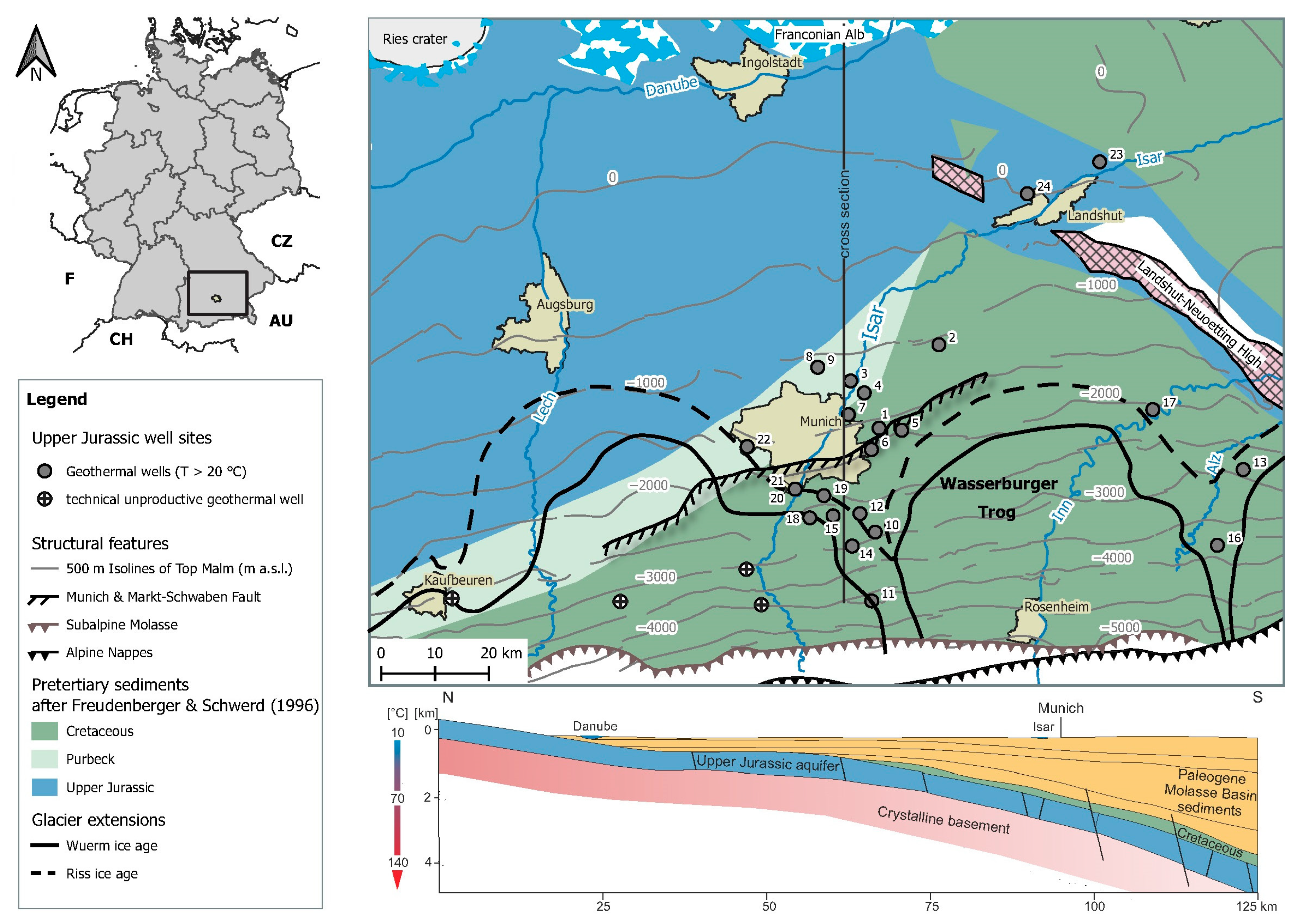
2. Geological and Hydrogeological Setting

The South German Molasse Basin (SGMB) is an alpine foreland basin located between the Alps in the south, the Upper Jurassic Franconian and Swabian Alb in the north and west and the Bohemian Massif in the east. The basin consists of alternating Cenozoic sequences of shallow marine and terrestrial, fluviatile Tertiary sediments such as sand-, clay- and limestones [45,46,47]. During Pleistocene, the Quaternary deposits were dominated by glaciers with great extensions and thicknesses over 1000 m in the southern SGMB (Figure 1) [48].
Figure 1. Study area of the central South German Molasse Basin with sampling points, distribution of the pretertiary sediments overlying the Upper Jurassic sediments [46] and geologic cross section (modified after [48]).
Water 13 01162 g001
The Upper Jurassic rocks are inclined to the south caused by the Alpine orogenesis to a depth about 6 km at the fringe of the Alps (Figure 1) and form an aquifer with a thickness of 400 to 600 m [48]. The Upper Jurassic aquifer is covered by Tertiary or partly Mesozoic sediments of the Purbeck and Cretaceous [45,46] (Figure 1).
In the main prospect areas, the complex karstified and fractured porous Upper Jurassic aquifer is composed of carbonate rocks such as small-pored limestones and fine- to coarse-grained dolostones [40]. Normal faults parallel to the Alps are crossing the Upper Jurassic aquifer [4,49], whereas the Munich and Markt-Schwaben Fault (MSF) represents an important major fault system for the geothermal exploration. Well tests showed partly very good hydraulic and thermal properties with groundwater temperatures up to 155 °C in the southern part of the SGMB [50,51]. Rock matrix porosities range from <1 to 20%, and hydraulic permeabilities vary between 0.01 and 1013 mD [3,4,41,52,53].
The thermal water composition in the Upper Jurassic aquifer changes from recently recharged low mineralised Ca-Mg-HCO 3 waters at the margin of the SGMB to higher mineralised ion-exchange waters of Na-HCO 3 -Cl, Na-Cl-HCO 3 and Na-Cl type after [54] with sodium as the dominant cation in the central basin [34,35,37]. Apparent water ages determined with 81 Kr at three geothermal wells ranged from 60,000 to 135,000 years in the central SGMB [44]. The occurring gas is mainly composed of CH 4 , CO 2 and N 2 , and reaches concentrations of maximum 2 L gas per litre water with gas phase proportions of sour gas (H 2 S) of a maximum of 5 vol% [38,43]. The provenance of hydrocarbons in the SGMB can be found in the overlying Tertiary hydrocarbon reservoirs with various source and mother rocks or particularly in the Upper Jurassic reservoir with a Mesozoic origin [33,55].
Previous work in this study area by several investigators led to different and partially contradicting concepts of groundwater recharge areas and groundwater flow systems of the Upper Jurassic aquifer:
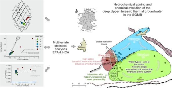
  • It was assumed that the recharge areas of the Upper Jurassic groundwater are located at the north-western boundary of the SGMB in the Swabian Alb. The general flow regime was determined by hydraulic potential analysis to be along the river Danube with a flow direction to the east and in direction to the central SGMB [25,36,37]. Observed higher mineralised ion-exchange waters at the north-eastern margin showed some evidence of groundwater flow from the central basin to the north-east of the SGMB [34,35];
  • The connate Upper Jurassic formation water was washed out of the aquifer. The low mineralised groundwater in the central SGMB was believed to be a mixture of meteoric water and higher mineralised formation or oil field waters, presumably seeping from the overlying Tertiary sediments, which are responsible for the higher and dominating amounts of sodium and chloride [2,24,25,29,31,33,37,38,56]. Subsequently, on the basis of the assumed geochemical evolution of the Upper Jurassic groundwater in the central SGMB, it was assumed that the groundwater flows from west to south-east towards the Alps [37];
  • The concept of subglacial recharge and cross-formational flow in the south-west of the SGMB (lake Constance region) and ion-exchange of paleo-water with an assumed northwards flow direction to the draining river Danube by [32,57] was recently supported by groundwater dating results derived from 81 Kr [44] and 14 C D O C [58]. Based on these results, recharge areas for the Upper Jurassic groundwater in the central SGMB were postulated to be at the northern fringe of the Alps, or south of the Northern Calcareous Alps [26].

3. Materials and Methods

3.1. Groundwater Sampling and Analysis

To conduct a comprehensive classification analysis of the deep thermal water, sampling was conducted at 22 deep geothermal production wells and two deep groundwater research wells, where no recent production takes place, in the central SGMB between January 2017 and June 2020. The geothermal wells are screened in the confined Upper Jurassic aquifer in depths between 1800 and 5000 m total vertical depth (mTVD). The water samples of the geothermal wells were obtained during the continuous operation with operating pressures up to 18 bar. During this study, no gas separation was performed prior to sampling. Because the temperature of the thermal waters ranged between 60 and 150 °C, water samples were cooled below 60 °C with a mobile heat-exchanger using high-temperature and high-pressure steel-teflon tubes and stainless steel fittings. Water samples of the two groundwater research wells with depths of 537 and 796 mTVD were taken after the water volume of the wells had been replaced at least twice and physico-chemical parameters (specific electrical conductivity (EC), pH-value and redox potential) were stabilised [59].
Samples for major anions and cations, trace elements, stable water isotopes (δD, δ 18 O), strontium isotopes ( 87 Sr/ 86 Sr), noble gases (Ne, He, Ar, Kr, Xe), as well as noble gas isotopes of helium ( 3 He/ 4 He) and argon ( 40 Ar/ 36 Ar) were collected and stored prior to analysis. The physico-chemical parameters pH-value, EC, temperature and redox potential were measured on site with a set of WTW Multi 3430 sensors (Xylem Analytics, Weilheim, Germany) directly at the outflow of the wells.

3.1.1. Water Chemical Parameters

Water samples for major ions and trace elements were field-filtered with a 0.22 μm filter, stabilised and stored in HDPE vials prior to analysis. Sub-samples for cations were acidified (HNO 3 (65%) and cooled (4 °C)) and anions were frozen. Major ions were analysed using an ion chromatograph Dionex ICS1100 (Thermo Fisher Scientific, Waltham, MA, USA) with an analytical precision <±5%. The trace element bromide was analysed using an ion chromatograph Dionex IC25 (Thermo Fisher Scientific, Waltham, MA, USA) and lithium, rubidium and strontium using a flame atomic absorption spectrometry (AAS 3300, Perkin Elmer, Waltham, MA, USA) at the Institute of Water Chemistry (IWC, Technical University of Munich). Detection limits were 0.1 mg/L for bromide and 0.01 mg/L for lithium, rubidium and strontium with an analytical precision <±5%. Samples for boron analyses were filled to the brim in 500 mL HDPE bottles and analysed after filtration (0.45 μm) using a spectrophotometer (Double Beam UV-190, Shimadzu, Duisburg, Germany) with a detection limit of <0.25 mg/L.
The DOC samples were field-filtered with a 0.45 μm filter and stored in brown glass vials, acidified to pH 2 with HCl (10%), and cooled (4 °C) prior to analysis with a catalytic high-temperature combustion method (Multi N/C 3100, Analytik Jena, Jena, Germany). The analytical error was <±5%.
The carbonate species HCO 3 and H 2 CO 3 were determined by titration with 0.1 M HCl and NaOH on site, with an approximate analytical error of ±0.1 mmol/L (6.1 mg/L for HCO 3 and 4.4 mg/L for H 2 CO 3 ).

3.1.2. Stable Water Isotopes

Samples for stable water isotope measurements were filled to the brim into 15 mL or 50 mL HDPE vials and an activated charcoal pellet was added to remove hydrocarbons from the water samples. The hydrogen and oxygen isotope ratios were determined after filtration (0.22 μm filter) in the laboratory of the Chair of Hydrogeology at the Technical University of Munich with a stable water analyser IWA-45EP (Los Gatos Research, San Jose, CA, USA) and were expressed in the δ notation (Equation (1)) with respect to the international standard VSMOW (Vienna-Standard Mean Ocean Water):
δ ( ) = R s a m p l e R S t a n d a r d R S t a n d a r d   ×   1000
where R stands for 2 H/ 1 H and 18 O/ 16 O ratios of the sample and standard, respectively. The analytical precision was ±1 ‰ for δD and ±0.1 ‰ for δ 18 O.
The global meteoric water line GMWL (δD = 8 × δ 18 O + 10 ‰) [60] represent the stable water isotope signatures of global precipitation and can be used to determine a meteoric origin of groundwater and temperature dependent effects during recharge or water-rock interaction [61]. The local meteoric water line LMWL (δD = 8 × δ 18 O + 8 ‰) of Garmisch-Partenkirchen [62] is representative for the precipitation in the study area at the foot of the Alps.

3.1.3. Strontium Isotopes

The samples for strontium isotopes were filled in 15 mL LDPE or 50 mL HDPE vials and 87 Sr/ 86 Sr isotope ratios were measured by thermal ionisation mass spectrometry (TIMS) VG Sector 54 (Micromass, Manchester, UK) in the laboratory of IsoAnalysis UG (Berlin). The TIMS raw data were evaluated using the international conventional method [63]. Mass fractionation was corrected using an 86 Sr/ 88 Sr ratio of 0.1194 and the 87 Sr/ 86 Sr data were normalised to a 87 Sr/ 86 Sr ratio of 0.71025 for NIST SRM 987. The accuracy and reproducibility were controlled with the analysis of the seawater standard IAPSO and the 2SD in-run-precision was <1.5 × 10 5 .

3.1.4. Noble Gases, 3 He/ 4 He and 40 Ar/ 36 Ar

Samples for noble gas measurements were collected into copper tubes fixed on aluminium racks [64,65], which were connected with the sampling tubes via special ferrule fittings from Swagelok and closed vacuum-tight with stainless steel clamps.
For 12 samples, analyses of Ne, 4 He and 3 He/ 4 He ratios were conducted at the noble gas laboratory of the Institute of Environmental Physics, University of Bremen, with a high resolution mass spectrometer MAP215-50 (Mass Analyser Products (MAP), UK) [64]. The analytical precision was better than ±1% for Ne and 4 He, and better than ±0.5% for 3 He/ 4 He.
The measurements of noble gas concentrations as well as isotopic ratios of 3 He/ 4 He and 40 Ar/ 36 Ar were performed for six samples with a mass spectrometer MM5400 (GV Instruments, Manchester, UK) at the Institute of Environmental Physics, Heidelberg University. The analytical precision of He and Ne ( 20 Ne) concentrations were ±1.1% and ±0.5%, respectively and for 3 He and thus 3 He/ 4 He ratios between ±3% and ±5%. For noble gas concentrations, the precision was better than ±1% for He and Ar and between ±1% and ±2% for Ne, Kr, and Xe. The argon isotope ratio was calculated directly in the mass spectrometer by alternately determining the signals of 40 Ar and 36 Ar in certain time periods and by using the absolute concentrations of the two isotopes to form the isotope ratio. The values given in Table 1 and Table A2 are the mean values of both methods.
Depending on the analysing institute, the copper tubes contained 5 g, 20 g (University of Heidelberg) or 40 g (University of Bremen) of the sample.

3.2. Calculation of Noble Gas Infiltration Temperatures (NGTs) Using Ne, Kr and Xe

The concentration of dissolved noble gases in groundwater are mainly controlled by the atmospheric input and convey information on physical properties of the water during air-equilibration at the air/water interface during recharge [66,67,68,69]. This information can be used for calculating the noble gas infiltration temperatures (NGTs) during groundwater recharge [68,70,71]. The NGTs were calculated using the program PANGA (Program for the Analysis of Noble GAs data) [72] and the closed system equilibration (CE) model [68] with Ne, Kr and Xe due to radiogenic contribution of He and Ar in the samples (Table 2). The fractionation parameters F were fitted and then subsequently the fractions of entrapped excess-air A were determined with a weighted least squares fitting approach and Monte Carlo simulations (5000 simulation runs) [73]. The used salinities varied according to their TDS and atmospheric pressure was set to 0.948 atm (infiltration at approximately 530 m above sea level) (Table A1).

3.3. Determination of Apparent Mean Residence Times with 4 He and 40 Ar

Helium and argon contents in basin aquifers consist of natural atmospheric background and terrigenous excess components. Both components are easily identifiable and the exchange of 4 He from rocks to fluid can be assumed to be fast [74]. Hypothetically, best estimates of the mean residence time could be determined by the accumulation of noble gas isotopes into groundwater with a uniform and constant rate per unit volume without any chemical reactions or diffusive exchange [75].
In general, the non-atmospheric, terrigenous excess helium fraction, 4 He e x , in a sedimentary basin is composed of the in situ produced 4 He i s by the radioactive α -decay of uranium and thorium in the aquifer rocks, and the external sources of the (deep) crustal 4 He c or mantle fluxes 4 He m [76,77]. These terrigenous as well as atmospheric sources in groundwater, such as air-equilibrated helium ( 4 He e q ) and dissolved air-bubbles ( 4 He a ), can be separated with the 3 He/ 4 He ratios and the Ne content [77]. The atmospheric 3 He/ 4 He ratio is R a 1.38 × 10 6 and is stored in air-saturated water (ASW) depending on salinity and temperature with R A S W 1.36 × 10 6 [78]. 3 He/ 4 He ratios of crustal origin (R c ) typically range between 0.01 R a and 0.1 R a [74,79,80]) and mantle-derived helium has typical values of R m between 5 and 10 R a [81]).
The 40 Ar/ 36 Ar ratios can be used to evaluate terrigenous 40 Ar e x component, which is composed of the radiogenic and in situ produced contribution from 40 K decay, 40 Ar i s , and the crustal fluxes ( 40 Ar c ) [82]. The atmospheric 40 Ar/ 36 Ar ratio R a ranges between 295.5 [83] and 298.5 [84]. Higher ratios point to a radiogenic 40 Ar e x input and accordingly long residence times [76].
The radiogenic excess helium 4 He e x and argon 40 Ar e x contributions can be used for groundwater dating [29,67,82,85,86,87,88]. The amount of excess 4 He e x accumulated in groundwater can be expressed as the non-atmospheric contribution 4 He n o n - a t m , which is calculated using the simplified Equation (2) under the assumptions that the proportion of the terrigenous component is considerably higher than the atmospheric 4 He component and that the difference between both the equilibrium and excess air 4 He components is also very small [89]:
4 H e e x 4 H e n o n - a t m = 4 H e m e a s N e m e a s N e e q   ×   4 H e e q ( c c S T P / g w a t e r )
with the measured 4 He m e a s and Ne m e a s concentrations and the equilibrium concentrations of helium 4 He e q = 4.90 × 10 8 ccSTP/g and neon Ne e q = 2.25 × 10 7 ccSTP/g under infiltration conditions at 0 C [78,90].
The excess 40 Ar e x component is calculated using Equation (3) [89]:
40 A r e x = 40 A r m e a s   ×   R m e a s R a R m e a s ( c c S T P / g w a t e r )
with the measured argon concentration 40 Ar m e a s , the measured and atmospheric 40 Ar/ 36 Ar ratios R m e a s and R a , respectively.
The in situ production rates P i (i = 4 He and 40 Ar) of the aquifer rocks are proportional with the content of the radiogenic elements uranium ([U] in ppm) and thorium ([Th] in ppm) for 4 He (Equation (4)) and potassium ([K] in weight%) for 40 Ar (Equation (5)) in the host rock. Accordingly, the accumulation rates A i , i s of in situ produced 4 He i s and 40 Ar i s can be calculated using Equation (6): [82]:
P 4 H e = 1.19   ×   10 13   ×   [ U ] + 2.88   ×   10 14   ×   [ T h ] ( c c S T P / g r o c k / y r )
P 40 A r = 3.887   ×   10 14   ×   [ K ] ( c c S T P / g r o c k / y r )
A i , i s = λ i   ×   1 ϕ ϕ   ×   ρ r o c k ρ w   ×   P i ( c c S T P / g w a t e r / y r )
with the production rates P i , the helium release factor λ i , the effective porosity ϕ of the rock, as well as the rock and water densities ρ r o c k and ρ w .
The time t e x required to produce the excess contribution C i , e x of 4 He e x and 40 Ar e x depends on the in situ accumulation rate A i , i s and the advective accumulation of crustal flux J i within the aquifer with a thickness z (in cm) and is calculated using Equation (7) [82,91,92]:
t e x = C i , e x A i , i s + J i ϕ   ×   z   ×   ρ w ( y r )
For the calculation of the in situ production rates P i , the accumulation rates A i , i s and the accumulation of crustal fluxes J i using Equation (7), mean values of the Upper Jurassic rock porosity ϕ = 0.1 and rock density ρ r o c k = 2.57 g/cm 3 [3]; uranium (U = 1.0 ppm), thorium (Th = 0.5 ppm) and potassium (K = 0.06 weight%) content [93]; an aquifer thickness of approx. 400 m; and assumed values for the water density ρ w = 1 g/cm 3 and release factors λ H e = λ A r of 1 were used.

3.4. Multivariate Statistical Techniques

Multivariate statistical techniques are very useful for data reduction and interpretation of large multi-constituent data sets [20,21,22,23,94] and have been used to identify distinct water types and unravel hydrogeological processes based on hydrochemical water composition. Clustering is an important tool for unbiased identification of patterns in a data set. Hierarchical cluster analysis (HCA) allows individual observations (objects) to be grouped into an indefinite number of clusters that aggregate together based on similarities [20,95]. Exploratory factor analysis (EFA) provides the basis to uncover the underlying structure of a data set consisting of a large number of inter-related variables and to reduce its dimensionality and complexity. By transforming the data with linear combinations to a new set of variables, the dimension of the data set is reduced to a number of significant factors that are responsible for most of the variation in the data set. A factor is indicated by the common shared variance of a set of variables and represents a process or construct [96,97].
All hydrochemical parameters (m = 17) of the n = 24 samples (Table A1 and Table A2), with the exception of noble gas data, which were not obtained for each well, were considered for HCA and EFA. The pH-values have not been used for the multivariate statistical analyses because they were not representative due to an affection by degassing of CO 2 and H 2 S during sampling. In addition, to reduce the complexity and increase the variance of the data set, the stable water isotope signatures of δD and δ 18 O, representing mainly infiltration conditions, evaporation and water-rock interaction processes, were combined to the SWI-dist parameter, which depicts the orthogonal distance from the GMWL. Thus, the data set was reduced to m = 17 parameters for the statistical analyses.
The HCA and EFA were performed and displayed with the statistical program R [98] using the integrated stats package and the packages psych [99], semTools [100] and ggplot2 [101].

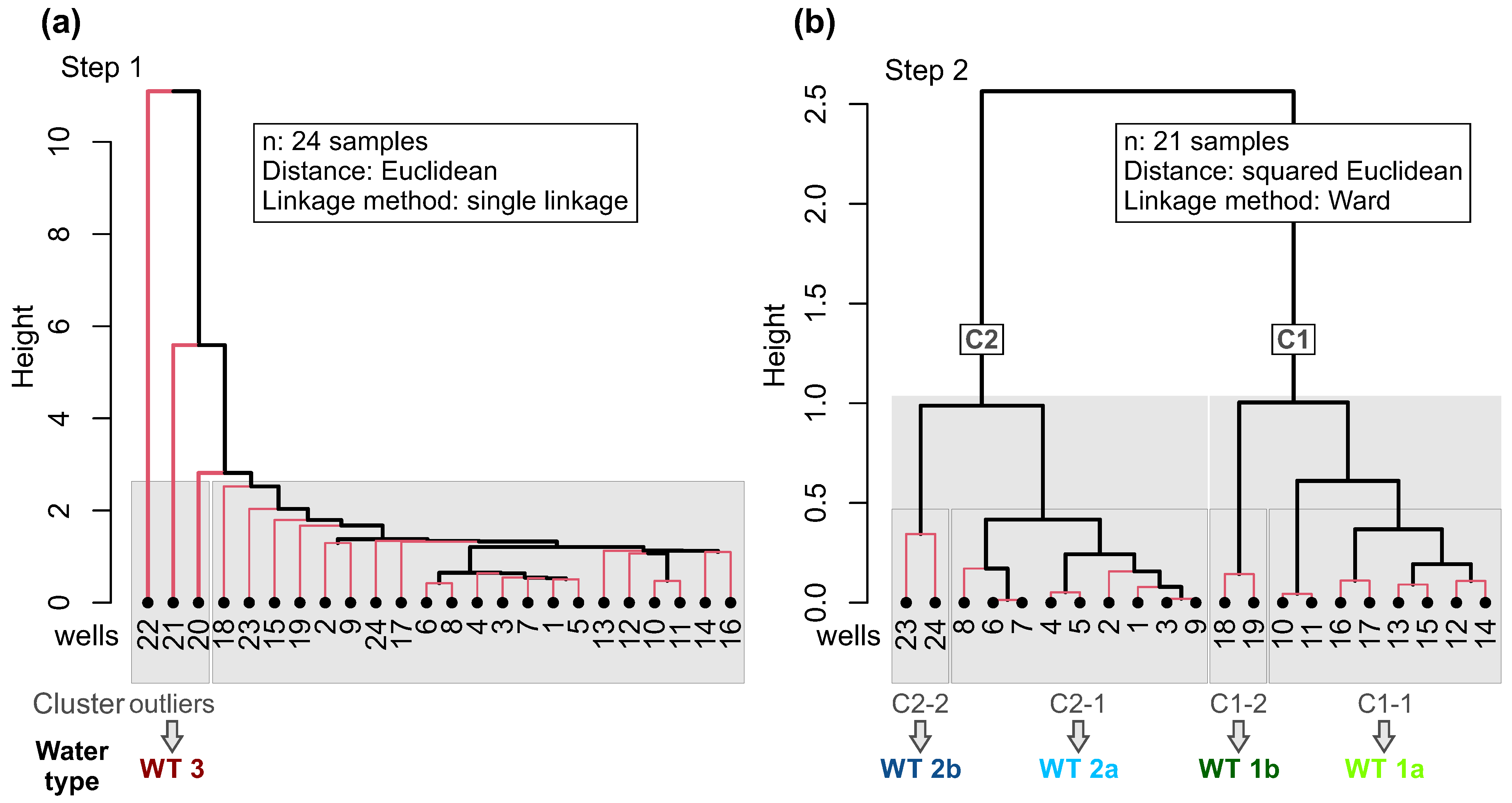
3.4.1. Hierarchical Cluster Analysis HCA

HCA was conducted with the z-standardised data set of m = 17 parameters of n = 24 water samples. The single linkage method (nearest-neighbour method) with Euclidean distance connects two points in a multi dimensional space with the closest distance [96,102,103], where the number of water samples (n) define the dimension. It can be used to detect outliers with the greatest distances to each other in the data set. To reduce the internal heterogeneity within the data set, the outliers were separated from the data set. Subsequently, the Ward’s linkage method using the minimum variance criterion and squared Euclidean distances was applied to find the most distinctive cluster with the lowest variance within the cluster [104]. To determine the optimal number of significant clusters, the “Elbow method”, “Silhouette method” and “Gap statistic” were applied using the packages factoextra [95] as well as NbClust [105] to compute 30 methods at once [95].

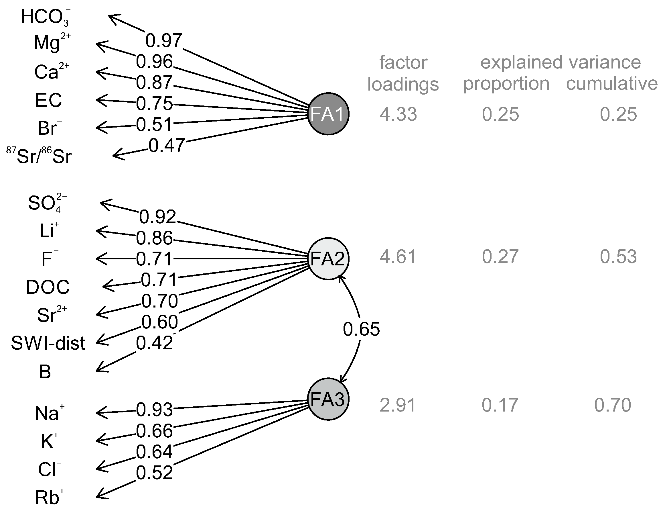
3.4.2. Exploratory Factor Analysis EFA

Prior to EFA, basic requirements were concerned for the same data set used for HCA of m = 17 parameters of n = 24 water samples [96]. The Shapiro-Wilk test of normality showed a non-Gaussian distribution of the z-standardised data set (p-values < 0.05 for every parameter except of F and 87 Sr/ 86 Sr ratio with p-values of 0.17 and 0.11, Table A5). Therefore, the ranked correlation matrix was calculated with Spearman’s ρ coefficient [102] (Appendix A.2, Table A4).
The suitability of the data set was tested prior to analysis (Table A5) with the Kaiser-Meyer-Olkin (KMO) test on the condition of a measure of sampling adequacy (MSA value) >0.5 [96]. The KMO test was statistically significant and showed a “middling” factor adequacy with an overall MSA value of 0.7. Bartlett’s test of sphericity with χ 2 of 371 indicated with a p-value of 1 × 10 23 < 0.05 overall statistically significant correlations within the correlation matrix. Cronbach’s α of 0.9 suggested a high internal consistency and reliability of the data set. The determinant of the correlation matrix was positive (1.7 × 10 10 ) indicating no non-positive definite matrix. Hence, the basic requirements for proceeding with EFA were achieved.
It is essential to determine the correct number of factors and, therefore, parallel analysis [106], Kaiser criterion (eigenvalues > 1) [107], empirical Kaiser criterion [108] and Scree test [109] were applied [110,111].

4. Results and Discussion

The results of all hydrochemical and noble gas analyses are presented in Table A1, Table A2 and Table A3 in Appendix A.1 and summarised in Table 1. All thermal waters were dominated by a mixture of sour gas (H 2 S) and aromatics such as hydrocarbons and some also had a separate oil phase. During sampling, degassing and separate phases of water and gas were observed at a few wells, particularly of samples 20 to 22.
The pH-values of all samples varied between 6.3 and 7.5 indicating slightly acidic to alkaline conditions. The chemical composition of the thermal waters differed between Na-Ca-HCO 3 -Cl, Na-HCO 3 -Cl, Na-Cl-HCO 3 and Na-Cl-type after Furtak and Langguth [54]. The mineralisation ranged from relatively low to highly mineralised groundwater with EC between 587 and 7702 μS/cm and showed a broad range of values for almost every parameter within the data set (Table 1). Therefore, the groundwater samples were clustered into distinctive groups that were deduced by the HCA.

4.1. Results of Multivariate Statistical Analyses HCA and EFA

4.1.1. Classification of Different Water Types of the Upper Jurassic Reservoir in the SGMB Based on HCA

The groundwater of the 24 sampled geothermal wells was clustered with the HCA to identify different groundwater types in the central SGMB [96,103]. The dendrograms in Figure 2 are the main results of the HCA. Based on the HCA of a first step (Figure 2a), three samples (20 to 22) were identified with the greatest single linkage Euclidean distance to the other samples in the data set. Although these three samples also differ among themselves, they may form a distinctive group due to their clear differentiation from the other samples. Therefore, they were separated from the data set.
The optimal number of significant clusters in the remaining data set ranged from two to four, depending on the method used. (Appendix A.3, Figure A1). However, in step 2 (Figure 2b), the remaining samples were clustered using Ward’s method and squared Euclidean distances and led to four different significant clusters, which is in accordance to the determined number of clusters using the “Elbow-method”. Thus, two main clusters could be clearly separated (with a relatively high distance measure): C1 and C2. In these clusters, further significant sub-clusters could also be distinguished, which resulted in four clusters C1-1, C1-2, C2-1 and C2-2. The interpretation of two main clusters and four subclusters is in good accordance to the range of optimal cluster numbers between two and four (Appendix A.3).
Subsequently, the water types were classified based on the results of HCA and the interpretation of the hydrochemical composition. Cluster C1 was defined as water type 1 with the subdivision of subtypes 1a (C1-1) and 1b (C1-2) and cluster C2 as water type 2 with the subdivision of subtypes 2a (C2-1) and 2b (C2-2). The outliers were summarised as water type 3 (Figure 2).

4.1.2. Identification of Factors and Hydrogeological Processes Affecting the Hydrochemical Water Composition

Factor analysis was performed and resulting factor loadings (see Section 3.4.2 and Appendix A.4) were used for detecting dependencies between each parameter and to reveal underlying hydrogeological processes that influence the hydrochemical composition and, thus, the results of HCA of the thermal waters.
EFA using multi-likelihood method and oblique (oblimin) rotation indicates that the system is driven by three statistical significant factors, which explain a variance of 70% in the data set (Figure 3, Appendix A.4). The factor loadings were 4.33 for FA1, 4.61 for FA2 and 2.91 for FA3 (Table A5). With the data set parameters used, the three factors are not capable of explaining the total variance of the entire data set and, therefore, may not cover all hydrogeological processes that influence the hydrochemical composition of thermal groundwater.
The explained variance, communalities h 2 , for the parameters ranged between 0.26 ( 87 Sr/ 86 Sr) and 0.94 (HCO 3 , SO 4 2 ) (Table A5). The not explained variance (u 2 ) for the parameters 87 Sr/ 86 Sr, F , Br , Sr 2 + and B was therefore greater than the explained variance (h 2 ), which accords to the not explained variance of 30% (Table A5). This implies that these parameters either describe or may be influenced by additional hydrogeological processes that are not characterised by the three factors, and that they may have only minor informative value for the processes described by the factors.
The factor FA1 contains six parameters (Figure 3) and may not only be related to one specific process. FA1 is represented by the earth-alkali metals Ca 2 + and Mg 2 + and, corresponding, HCO 3 , which can be linked to the “hardness” or “alkalinity” of the water. The mineralisation, which is expressed by EC, is also mainly a proxy for FA1 and, therefore, may be more influenced by the earth-alkali elemental system rather than the salinity (FA3). Moreover, as Br is a proxy of FA1 and not of FA3 such as Na + and Cl , this may prefigure that the dominant processes on the salinity (NaCl) of the thermal water was not necessarily controlling the bromide content in groundwater. This could indicate different hydrogeological processes affecting the mineralisation and especially the salinity of the thermal waters.
The 87 Sr/ 86 Sr ratio as an indicator for specific water-rock interaction is also a proxy of FA1, but shows only a relatively low factor loading (0.47) compared to the other parameters of FA1. However, the 87 Sr/ 86 Sr ratios are not a proxy for the same factor than Sr 2 + , which is often associated with Ca 2 + in carbonate rocks [112]. As a consequence, this may suggest that the 87 Sr/ 86 Sr ratios of the thermal water may be influenced by different processes or additional sources, as indicated by their high u 2 (Table A5), and that the 87 Sr/ 86 Sr signature may not necessarily linked to the strontium uptake from carbonate rocks.
FA2 links SO 4 2 , Li + , F , DOC, Sr 2 + , SWI-dist and B. Due to the correlation of B and DOC, B is likely controlled by the DOC mobility and, therefore, likely by the petroleum genesis [113]. Therefore, DOC and B together with F and SO 4 2 may describe the influence of hydrocarbons from oilfield waters or methanogenesis induced by thermochemical sulphate-reduction (TSR) [38,114] as main process of FA2. These processes are probably linked to the information of the parameter SWI-dist, which corresponds to the meteoric origin on the one hand and the water-rock interaction of the thermal water on the other hand. Therefore, it can be concluded that a deviation of the stable water isotope signatures from the GMWL can mainly be caused by the influence of oilfield waters and corresponding organic (reduction) processes [61].
FA3 is among others dominated by Na + and Cl , which control the “salinity” (NaCl) of the thermal water. The parameters Na + , K + and Rb + are also proxies for interaction processes with silicate and likely clay minerals [115], which may correspond to “ion-exchange processes” in the thermal water.
The factors FA2 and FA3 correlate with a R 2 of 0.65 indicating a common shared variance. This suggest that a portion of the salinity of the thermal water may also be related to the influence of oilfield waters and water-rock interaction.
Gypsum (CaSO 4 ) dissolution as a possible considerable process on the thermal water composition is not necessarily implied by the EFA. The significant factor loadings of Ca 2 + and SO 4 2 are proxies of different factors, which is in accordance to the lithologic composition of the aquifer rocks [38] (Section 2).
Carbonate dissolution as a dominant reaction that affects the concentration of B may have no or only a little effect [116] as both parameters DOC and B are proxies of FA2 and do not show a relation to the parameters Ca 2 + , Mg 2 + and HCO 3 , which are proxies of FA1.

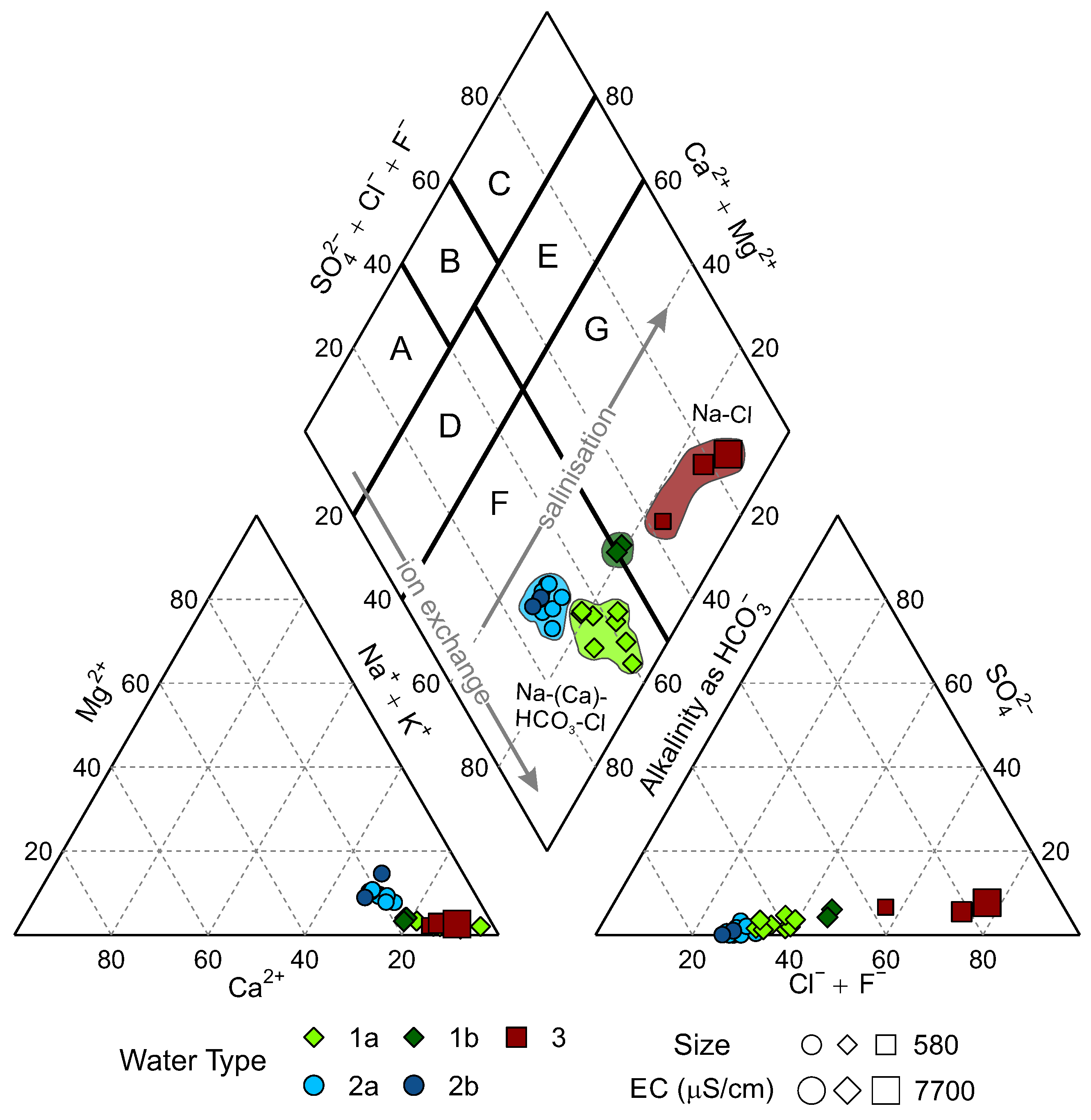
4.2. Chemical Analyses of Grouped Water Types
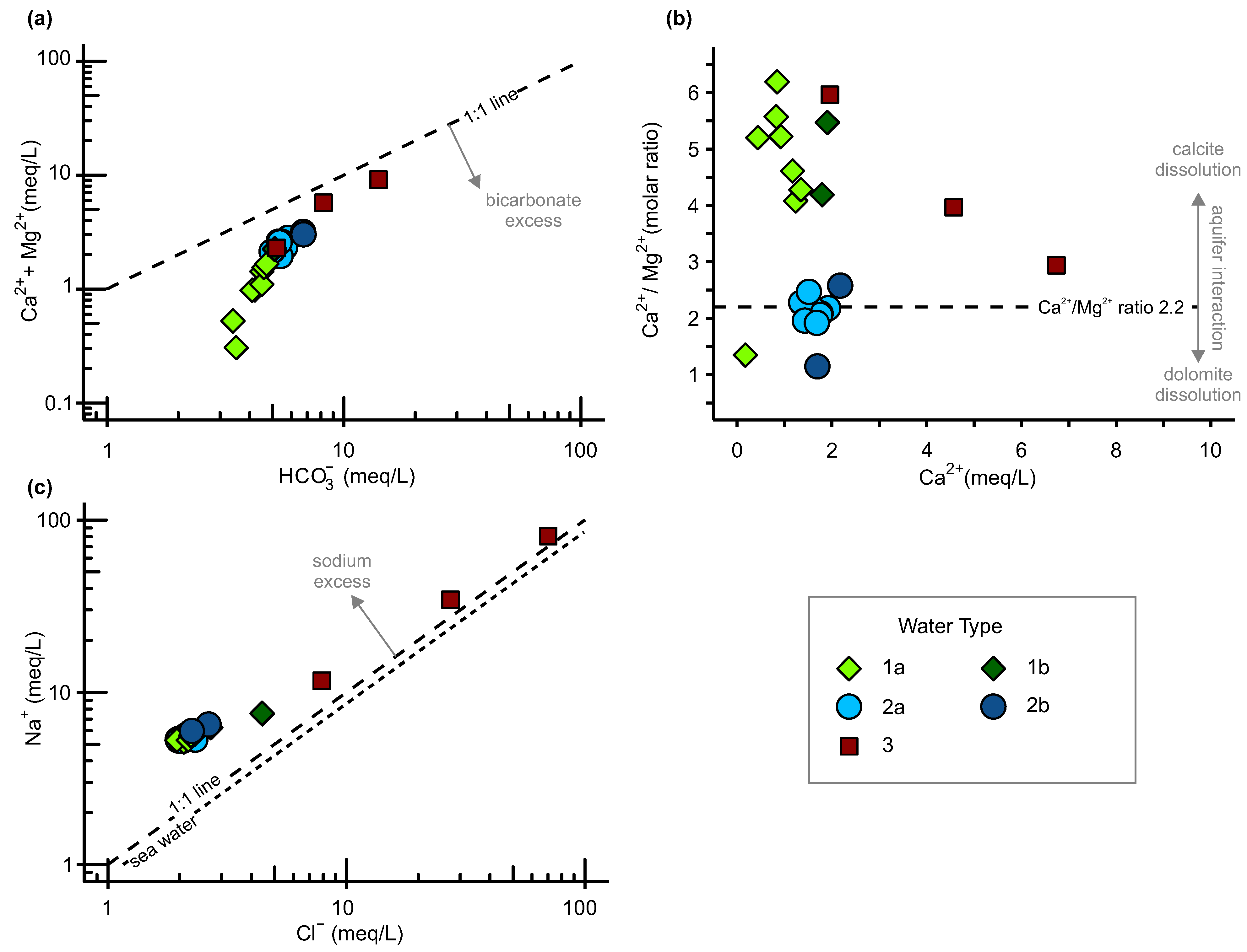
Table 1 summarises the hydrochemical parameters for the complete data set and each clustered water type with minimum, maximum and mean values. The hydrochemical facies after [54] of the water samples is displayed in the Piper plot with the EC as scale for the symbol size (Figure 4).

4.2.1. Water Type 1

The groundwater of water type 1 represent alkaline waters with a bicarbonate and chloride domination (field F and G in Figure 4) and was classified as Na-HCO 3 -Cl water [54]. The water type 1 was separated due to the results of HCA into two subtypes, 1a and 1b (Section 4.1.1).
For water type 1a, the mean concentrations were 5.60 ± 0.36 mmol/L for Na + and 2.23 ± 0.23 mmol/L for Cl (Table 1). The concentrations of Ca 2 + ranged from 0.09 to 0.67 mmol/L (mean value 0.43 ± 0.20 mmol/L), the concentrations of Mg 2 + varied between 0.04 and 0.16 mmol/L (mean value 0.10 ± 0.04 mmol/L) while HCO 3 showed concentrations between 3.4 and 4.7 mmol/L (mean value 4.2 ± 0.5 mmol/L).
Water type 1b samples were more mineralised with an EC between 1029 and 1087 μS/cm compared to the samples of water type 1a (mean value 671 ± 55 μS/cm). The difference in mineralisation between the subtypes 1a and 1b is mainly caused by the considerably elevated salinity as main process of FA2 (mean values: Na + 7.54 ± 0.03 mmol/L; Cl 4.44 ± 0.01 mmol/L) and elevated alkalinity as proxy of FA1 (mean values: Ca 2 + 0.92 ± 0.04 mmol/L; HCO 3 5.1 ± 0.0 mmol/L) for type 1b. The mean Mg 2 + concentration (0.19 ± 0.02 mmol/L) for type 1b was comparable but only slightly elevated to the values of water type 1a (Figure 5a,b, Table 1). For samples of both subtypes 1a and 1b, the concentrations of K + (between 0.40 and 0.82 mmol/L), F (between 0.11 and 0.41 mmol/L) and SO 4 2 (between 0.04 and 0.32 mmol/L) were only subordinately represented.
Overall, both subtypes of water type 1 showed dominant influences of ion-exchange processes between Ca 2 + and Na + (Figure 4 and Figure 5a,c). Although Na + and HCO 3 showed an excess compared to Cl , Ca 2 + and Mg 2 + (Figure 5a,c), a positive trend of increasing HCO 3 with Ca 2 + and Mg 2 + concentrations was observed (Figure 5a). The concentrations of B and DOC, which may indicate influences of oilfield waters as a process of FA2 were relatively low between 0.08 and 0.31 mmol/L for B and 1.48 to 4.20 mg/L for DOC.
It can be concluded that the water chemical composition of water type 1b is comparable to water type 1a, but shows considerably higher levels of mineralisation, alkalinity and salinity, which may indicate hydrogeological processes influencing the hydrochemical evolution of these waters.

4.2.2. Water Type 2

The Na-Ca-HCO 3 -Cl groundwater of water type 2 is very homogeneously distributed in field F of the Piper plot (Figure 4) and represent also alkaline waters with a bicarbonate and chloride domination after [54].
The EC for water type 2 ranged from 697 to 968 μS/cm with mean values for subtype 2a of 723 ± 22 μS/cm and slightly higher for subtype 2b with 893 ± 103 μS/cm. Ca 2 + contents ranged between 0.68 and 1.09 mmol/L (mean values: 0.81 ± 0.09 mmol/L (type 2a); 0.97 ± 0.17 mmol/L (type 2b)) and Mg 2 + concentrations varied from 0.30 to 0.74 mmol/L (mean values: 0.38 ± 0.05 mmol/L (type 2a) and 0.58 ± 0.22 mmol/L (type 2b)). The HCO 3 content of subtype 2b was also considerably elevated with a mean value of 6.7 ± 0.0 mmol/L compared to subtype 2a with 5.4 ± 0.3 mmol/L. The mean concentrations of Na + (5.33 ± 0.13 mmol/L (type 2a); 6.25 ± 0.38 mmol/L (type 2b)) and Cl (2.04 ± 0.12 mmol/L (type 2a); 2.45 ± 0.28 mmol/L (type 2b)) were slightly elevated for samples of subtype 2b compared to subtype 2a (Figure 5c). However, both subtypes showed dominant influences of ion-exchange processes between Ca 2 + and Na + due to the sodium and bicarbonate excess (Figure 4 and Figure 5a,c).
For groundwater of both subtypes 2a and 2b, the concentrations of K + (between 0.19 and 0.41 mmol/L), F (between 0.10 and 0.14 mmol/L) and SO 4 2 (between 0.00 and 0.14 mmol/L) were only subordinately represented and generally lower than for type 1 waters. Oilfield water had probably no or only little effect on groundwater samples of type 2 which is documented by low concentrations of B between 0.05 and 0.23 mmol/L and DOC ranging from 0.50 to 0.23 mg/L.
Overall, the water chemical composition of both subtypes of type 2 were quite similar to each other with slightly higher levels of salinity and alkalinity, especially HCO 3 , for subtype 2b.
A considerable water chemical difference between the two water types 1 and 2 and their subtypes is expressed by their contents of calcium and magnesium, which were main proxies of the factor FA1 (Table A5), and, therefore, their Ca 2 + /Mg 2 + ratios (Figure 5b). A molar Ca 2 + /Mg 2 + ratio of 1 is caused by the dissolution of pure dolomite whereas higher ratios above 2.2 indicate an increasing influence of calcite dissolution in the aquifer [29,38,118,119]. The molar Ca 2 + /Mg 2 + ratios (Table 1) above 2.2 for water type 1 (mean values: 4.6 ± 1.5 for subtype 1a; 4.8 ± 0.9 for subtype 1b) may indicate some influences of calcite dissolution from the rocks within the basin. In contrast, the molar Ca 2 + /Mg 2 + ratios around 2.2 for type 2 water samples (mean values: 2.1 ± 0.2 for subtype 2a; 1.9 ± 1.0 for subtype 1b) clearly indicate some influences of dolomite dissolution from the rocks within the basin.

4.2.3. Water Type 3

Water type 3 showed a broad range of EC from 1596 to 7702 μS/cm with a mean value of 4366 ± 3092 μS/cm (Table 1). The major chemical parameters of the groundwater samples of type 3 plot heterogeneously distributed in field G of the Piper plot (Figure 4), which represent alkaline waters with a chloride predomination (Na-Cl and Na-Cl-HCO 3 type). They plot clearly distinguishable from the other water types and also show great heterogeneity among themselves.
The Ca 2 + concentrations varied from 0.98 to 3.37 mmol/L and Mg 2 + concentrations ranged between 0.16 and 1.19 mmol/L. Contrary to water types 1 and 2, the samples of water type 3 were characterised by a predominant influence of the salinity (Na + and Cl ), which was defined as one main influence of the factor FA3 (Section 4.1.2). The concentrations ranged from 11.70 to 80.64 mmol/L (mean value 42.27 ± 35.13 mmol/L) for Na + and varied between 7.88 and 70.10 mmol/L (mean value 35.10 ± 31.83 mmol/L) for Cl . With increasing concentrations of Na + and Cl , the groundwater samples of water type 3 converge to the 1:1 line in Figure 5c, but showed as well predominant ion-exchange processes between the alkali ion Na + and the earth-alkali ions Ca 2 + and Mg 2 + (Figure 5a,c). The molar Ca 2 + /Mg 2 + ratios ranged from 2.9 and 6.0 indicating distinct interaction between the fluid and calcite minerals. Interestingly, with increasing Ca 2 + concentrations, the Ca 2 + /Mg 2 + ratio decreases indicating a higher influence of dissolved dolomites. Similar results have been found for the Pannonian geothermal aquifer where comparable water evolution trends were observed [18].
The clearly elevated concentrations of B (between 0.81 and 3.24 mmol/L) and DOC (4.43 to 70.49 mg/L) may indicate as proxies of FA2 additionally considerable influences from oilfield waters. The concentrations of major ions K + , F and SO 4 2 were also consecutively elevated and ranged between 0.89 and 2.18 mmol/L for K + , between 0.12 and 0.27 mmol/L for F and between 0.47 an 1.84 mmol/L for SO 4 2 .

4.3. Assessing Recharge Conditions and Water Rock Interaction

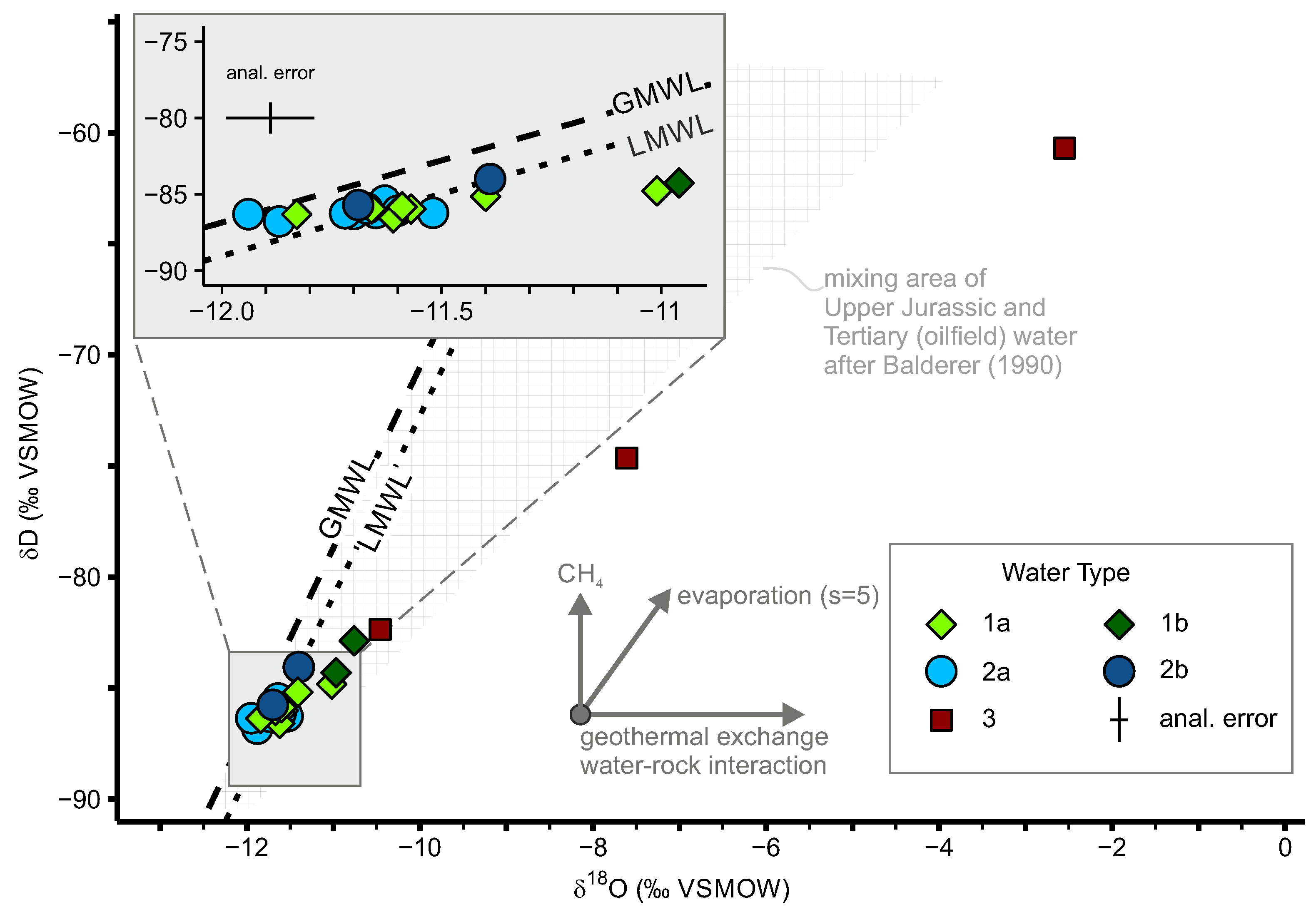
4.3.1. Noble Gas Infiltration Temperatures NGTs and Stable Water Isotopes

The NGTs were calculated to obtain the temperature-driven recharge conditions of representative samples for each water type (Table 2). The calculated entrapped excess-air A ranged for the samples 9 (type 2a), 16, 17 (both type 1a) and 18 (type 1b) between 0.23 and 0.36 ccSTP/g. These values are above the expected values for groundwater [68] and could possibly be explained with equilibration between groundwater and trapped air bubbles [72] or infiltration under overburden pressure. The fractionation parameters F were fitted with the CE-Model [68] and ranged between 0.94 and 0.98 for both subtypes of type 1 and 2a waters. They are within a reasonable range but also indicate most probably degassing of the samples as they were close to 1. However, it was not possible to calculate reasonable NGTs for the two samples of type 3 due to inappropriate noble gas mass balances and negative values for A (Table 2) [72].
The stable water isotopes are capable of storing information regarding the climate conditions during infiltration or (geothermally driven) water-rock interactions in the subsurface [117,120,121]. In addition, the mixing range of stable water isotope signatures from literature data [31,32] for Upper Jurassic and Tertiary Molasse Basin oilfield waters shown in Figure 6 can be used to assess the nature of the water-rock interaction.
The stable water isotope signatures of both water types 1 and 2 are very homogeneously distributed with δD ranging from −86.8 to −82.8 ‰ and δ 18 O values between −12.0 and −11.0 ‰ (Table 1). They scatter in Figure 6 predominantly between the GMWL and LMWL indicating meteoric origin.
Especially the stable water isotope signatures of water type 1a and both subtypes of 2 indicate a meteoric cold climate origin that is typical for Pleistocene waters in that region [122]. This is supported by the results of NGTs between 0.9 ± 0.5 °C and 1.4 ± 0.5 °C for water types 1a and 2a (Table 2). These results are in good accordance to a previously determined NGT (2.8 ± 0.5 °C) of groundwater from a Upper Jurassic geothermal well in this study area [35,123]. Results of noble gases stemming from other deep basins such as the Pannonian Basin also indicate comparable recharge conditions during the Pleistocene glacial period with NGTs below 4 °C [8]. The distances to the GMWL, SWI-dist, ranged between 0.09 and 0.82 with mean values of 0.43 ± 0.18 for type 1a, 0.31 ± 0.11 for type 2a and 0.30 ± 0.06 for type 2b. These values do not imply considerable isotope exchange processes of hydrogen and oxygen during evaporation or with soil or bedrock after recharge.
In contrast, the stable water isotope signatures of two samples of water type 1b with δD values of −84.3 and −82.8 ‰ and δ 18 O values of −11.0 and −10.8 ‰ plot slightly below the LMWL and were more isotopically enriched compared to the remaining samples of water types 1a, 2a and 2b. The observed enrichment of δ 18 O values and, corresponding, the slightly elevated mean value of SWI-dist (0.82 ± 0.02, Table 1) are typical for geothermally driven oxygen exchange due to water-rock interaction with carbonate rocks in sedimentary basins [61,120]. The NGT of the water type 1b sample is elevated with 3.1 ± 0.5 °C compared to the other samples of type 1a and 2, but indicates together with the stable water isotope signatures meteoric Pleistocene cold climate infiltration conditions [122]. Thus, it can be concluded that water type 1b has probably been influenced by geothermal isotope exchange due to water-rock interaction after recharge during the Pleistocene. Mixing processes between Pleistocene water and fossil formation water that led to this additional isotopic shift in δ 18 O could also be a reasonable explanation.
The elevated entrapped excess-air A of both water types 1 and 2 point to an infiltration under overburden pressure, which may indicate a subglacial groundwater recharge [65] (Table 2). This is also in accordance to apparent 81 Kr ages between 60,000 and 135,000 years for some type 1a and 2a water samples [44], which point to a recharge during the Riss (300,000 to 130,000 years) and Wuerm (115,000 to 11,700 years) glaciations. However, this suggests that the altitude effect had most likely no or only little influence on the stable water isotope signatures for type 1 and 2 waters.
For water type 3, the δD values ranged between −82.3 and −60.6 ‰ and δ 18 O values ranged from −10.5 to −2.6 ‰ (Table 1). The stable water isotope signatures plot heterogeneously distributed and clearly below both meteoric water lines (GMWL and LMWL) in Figure 6. The initial recharge conditions of water type 3 can therefore not be delineated. The orthogonal distances to the GMWL (SWI-dist), ranging from 1.07 to 6.23, may indicate extensive water-rock interaction, as already suggested by the water chemical composition (Section 4.2). These stable water isotope signatures are typical for highly mineralised evaporated brines in deep sedimentary basins [61,120] and oil- and gasfield waters in the Molasse basin [31,33,124]. They plot both inside and slightly outside of the mixing area of Upper Jurassic and Tertiary (oilfield) waters (Figure 6), which illustrates the influence of water-rock interaction together with methanogenesis. The inappropriate noble gas mass balances indicate that the samples were most probably affected by the observed separate fluid phases and/or degassing processes during sampling [72]. Thus, this also implies considerable influences of oilfield waters to water type 3.

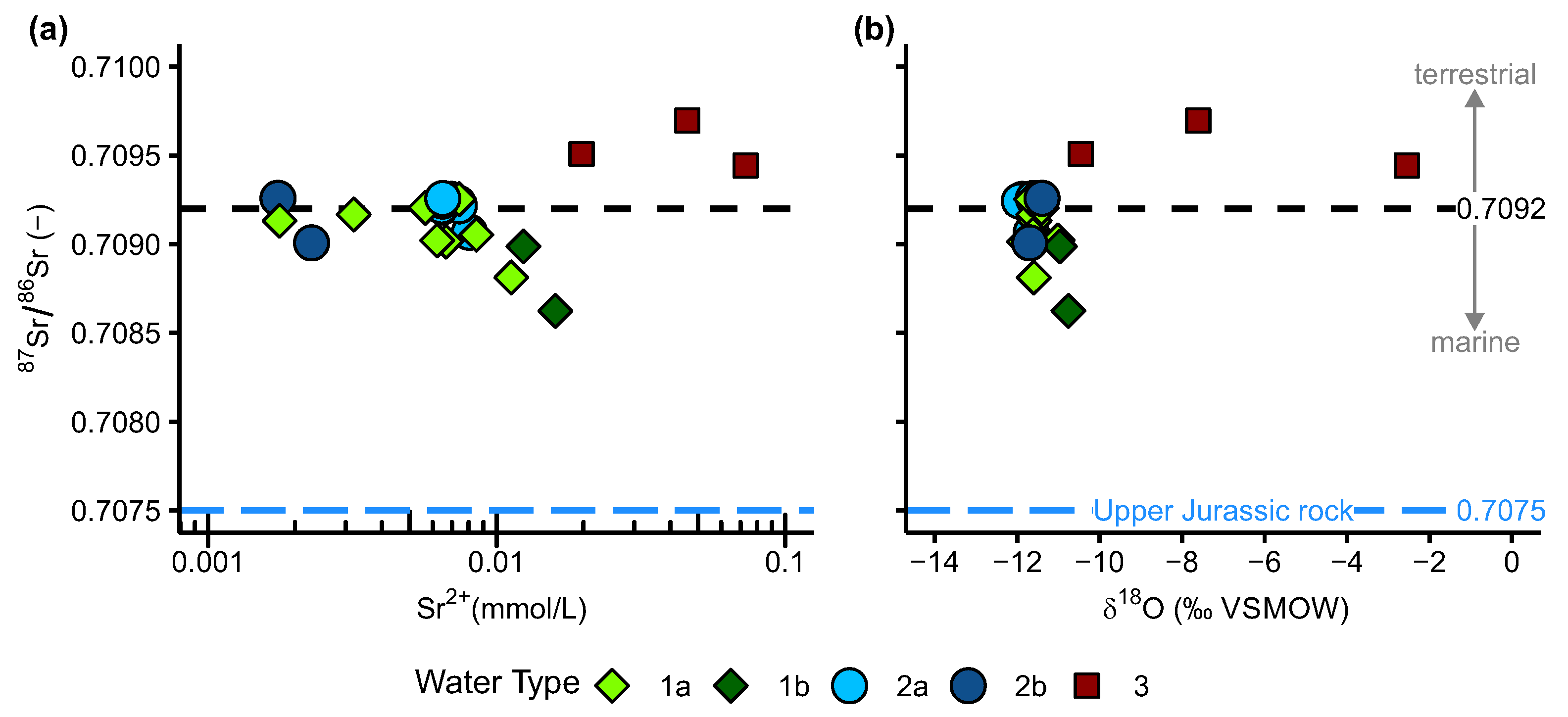
4.3.2. Tracing Water-Rock Interaction with 87 Sr/ 86 Sr Signatures

The 87 Sr/ 86 Sr ratio of groundwater is a very useful tracer to determine the dependency of water-rock interaction and mixing processes influencing the water chemical composition of the different water types [125,126,127]. The 87 Sr/ 86 Sr signature of groundwater depends on the chemical evolution during recharge and infiltration through the unsaturated zone, the aquifer lithology, the rocks alteration level and intensity of water-rock interactions. Infiltrating water receives its 87 Sr/ 86 Sr signature in the soil zone, which is then not fractionated and preserved unless mineral dissolution of the aquifer host rocks occur [128].
The mean 87 Sr/ 86 Sr ratios of water type 1, 0.70908 ± 0.00014 (type 1a) and 0.7088 ± 0.00026 (type 1b), and water type 2, 0.70921 ± 0.00006 (type 2a) and 0.70913 ± 0.00018 (type 2b), were clearly above the characteristic mean values of the Upper Jurassic carbonate rocks of the SGMB, which are around 0.7075 [93]. The radiogenic 87 Sr/ 86 Sr ratios are relatively constant and independent of the strontium content for type 1 and 2 waters with Sr 2 + < 0.008 mmol/L (Figure 7a). This indicates that the strontium isotope chemistry of these waters was not predominantly influenced by the dissolution of Upper Jurassic carbonate rocks after recharge. With increasing Sr 2 + concentrations > 0.008 mmol/L, the type 1a waters show clearly decreasing 87 Sr/ 86 Sr ratios. Moreover, the water type 1b samples with higher Sr 2 + concentrations ranging from 0.012 to 0.016 mmol/L showed also considerably lower 87 Sr/ 86 Sr ratios between 0.70862 and 0.70899. The higher Sr 2 + concentrations corresponding with lower 87 Sr/ 86 Sr ratios of these type 1a and especially type 1b waters may therefore indicate dissolution of calcite carbonates most likely from Upper Jurassic rocks.
Figure 7b shows an inverse relationship between decreasing 87 Sr/ 86 Sr ratios with enriching (less negative) δ 18 O values for samples of both water types 1 and 2. This relationship supports the hypothesis that interaction of groundwater with the Upper Jurassic rocks due to the geothermal exchange with the carbonate minerals [120] or fossil formation waters may have been responsible for the observed isotopic shift in δ 18 O (Figure 6).
The relationship of 87 Sr/ 86 Sr signatures with Sr 2 + concentrations and δ 18 O values of type 3 water samples in Figure 7a,b indicate a different influence on the hydrochemical composition and water-rock interactions compared to both water types 1 and 2. The 87 Sr/ 86 Sr ratios for type 3 waters are tending to more radiogenic signatures clearly above 0.7092 with values between 0.70941 and 0.70970. Subsequently, water type 3 was highly likely not dominated by the fluids in the rock matrix and rock geochemistry of the Upper Jurassic aquifer rock. The increased strontium concentrations between 0.020 and 0.073 mmol/L could therefore not be explained by the dissolution of marine carbonate rocks of the Upper Jurassic reservoir. As a result, the radiogenic 87 Sr/ 86 Sr ratios clearly indicate a strontium input from interactions with non-marine terrestrial rocks, fossil formation waters from terrestrial sediments, and also oilfield waters [130]. It can be suggested that this radiogenic influence on the 87 Sr/ 86 Sr signatures of water type 3 is related to a hydraulic contact to overlying terrestrial Tertiary sediments and Tertiary fossil formation water.

4.3.3. Mixing Processes and Origin of Salinity Using δ 18 O and Cl

Geochemically driven processes influencing the water chemistry and salinisation, such as mixing between fresh and highly saline fossil formation waters, can be differentiated by plotting the relationship of δ 18 O with the conservative ion Cl [9,33]. Based on the results so far, the mixing model was extended and adopted to the origin of salinity for water types 1b and 3 (Figure 8). A hydrogeochemical evolution of type 1a and 2 waters that interact with the Upper Jurassic carbonate rocks of the SGMB is represented by a mixing zone where highest and lowest saline fluid inclusion data stemming from the Upper Jurassic rocks [40] act as end members of the mixing model.
The samples of water type 1b plot along the mixing line of water types 1a and 2 that is characterised by the lower range of fluid inclusion values of Upper Jurassic rocks. This may indicate that the source of Cl in that water may be also related to the isotopic enrichment of δ 18 O (Section 4.3.1), which was assumed to be caused by geothermal exchange processes of type 1a water with the Upper Jurassic reservoir rocks (Section 4.3.2). The associated enrichment of δ 18 O with increasing Cl concentrations of type 1b waters may therefore indicate chloride uptake due to dissolution of the less saline Upper Jurassic carbonate minerals and also suggest an interaction with the fossil Upper Jurassic formation water that is stored in the rock matrix.
In contrast, the samples of water type 3 plot very heterogeneously distributed within the mixing zone of the mean values of type 1a and 2 waters with the upper and lower ranges of the Upper Jurassic rock and fluid inclusion data in Figure 8. The distinct isotopic enrichment of the δ 18 O values of water type 3 is accompanied by much more significant chloride uptake compared to water type 1b. The maximum values of water type 3 form a positive and linear mixing correlation with type 1a and 2 waters, which can be clearly differentiated from the mixing processes with seawater. As the samples of water type 1b do not plot on that linear mixing line, it is assumed that the origin of salinity is likely different compared to water type 3. Together with the results of the strontium isotopes (Section 4.3.2), an influence of higher saline Tertiary formation water leading to an increased salinity (Section 4.2) and stable water isotope signatures that are typical for sedimentary brines (Section 4.3.1) is highly suggested for water type 3.

4.4. Calculation of Apparent Water Ages by Radiogenic Noble Gas Isotopes

The noble gas isotope data were not considered in the multivariate statistical analyses as they were not obtained at every well in this study (Section 3.4), but they also provide useful information about influences of hydrogeological processes as well as apparent mean residence time of the thermal groundwater. Increased apparent groundwater ages would be an indication of the influence of fossil formation waters and could allow conclusions about higher water-rock interaction due to reduced hydraulic permeability.
The noble gas isotope analyses of the thermal water samples from the deep Upper Jurassic reservoir in this study were partially affected by varying high amounts of the dissolved gases (e.g., CH 4 , CO 2 , N 2 , H 2 S), and probably partial degassing during uplift at sampling temperature [71,82,131,132,133,134,135]. Equilibration of noble gases dissolved in water with the non-atmospheric gas phases of CH 4 and H 2 S could have induced undersaturation of the atmospheric signatures [82]. However, it is assumed that the isotope ratios 3 He/ 4 He and 40 Ar/ 36 Ar of the samples were not be considerably affected by these processes.
The 3 He/ 4 He ratios in Figure 9a indicate that all thermal groundwater samples were air saturated water that accumulated radiogenic 4 He e x of crustal origin (R c between 0.01 and 0.1 R a [74,79,80]) with no or only little evidence of mantle-derived 4 He m . The non-atmospheric portion of helium 4 He n o n - a t m for all samples is greater than 99 %. The 3 He/ 4 He ratios < 0.1 R a indicate considerable contributions from radiogenic 4 He e x and thus probably high apparent mean residence times [136].
The water samples of type 1a and 2a, which had overall no or only negligible separate gas phases, displayed relatively homogeneous 4 He concentrations of 2.27 ± 0.34 × 10 5 ccSTP/g and 2.21 ± 0.20 × 10 5 ccSTP/g, respectively (Table 1). The mean 3 He/ 4 He ratios were 1.03 ± 0.09 × 10 7 for water type 1a and 1.12 ± 0.14 × 10 7 for water type 2a, which comprise a very narrow range for both subtype samples. The 40 Ar/ 36 Ar ratios of around 300.1 (between 299.8 and 302.5) for the three samples of type 1a and 2a were close to the ASW signature ( 40 Ar/ 36 Ar 298.5 [84]) (Figure 9b) with subsequently only minor contributions of radiogenic 40 Ar e x between 2.17 and 6.65 × 10 6 ccSTP/g (Table A2).
For water type 1b, the 3 He/ 4 He ratios were lower compared to type 1a and 2a samples and ranged between 6.45 and 7.31 × 10 8 while the 4 He concentrations were higher varying from 4.22 × 10 5 to 1.58 × 10 4 ccSTP/g (Table 1). The considerably elevated 40 Ar/ 36 Ar ratio of 307.6 resulted in a higher 40 Ar e x concentration of 5.76 × 10 5 ccSTP/g (Table 3) compared to water type 1a and 2a. This indicates that the apparent groundwater age of water of type 1b may be higher than for water type 1a and 2a.
However, the determination of apparent residence times based on the radiogenic accumulation of 4 He and 40 Ar is very complex due to the unknown advective vertical crustal fluxes J 4 H e and J 40 A r of the underlying crustal rocks in the SGMB. For two samples of this data set of water type 1a (sample 16) and water type 2a (sample 9), the apparent 81 Kr ages are quite similar with 110,000 and 135,000 years, respectively [44]. Due to the almost identical radiogenic 4 He e x values and comparable 40 Ar e x values of these two samples, the crustal fluxes J 4 H e and J 40 A r were calculated under the assumption of a closed Upper Jurassic aquifer system using Equation 7. The resulting fluxes, J 4 H e 7.87 × 10 7 ccSTP/cm 2 /yr and J 40 A r 1.38 × 10 7 ccSTP/cm 2 /yr (Table 3), are within a comparable range of crustal fluxes from other studies for J 4 H e between 2.1 and 4 × 10 7 ccSTP/cm 2 /yr [87,91] and for J 40 A r between 0.3 and 1.1 × 10 6 ccSTP/cm 2 /y [137,138]. Since the fluxes were determined on only two samples of water type 1a and 2a, it had to be tested whether comparable apparent water ages could also be calculated by the assumed accumulation at the other wells with these water types where helium and argon were also determined. For this purpose, the mean values of the 40 Ar e x and 4 He e x of water types 1a and 2a were calculated and the apparent ages were determined for their minimum, maximum and mean values. Accordingly, with the mean values for all samples of water types 1a and 2a of 4 He e x 2.23 × 10 5 ccSTP/g and 40 Ar e x 4.41 × 10 6 ccSTP/g, apparent mean residence times between 112,000 (t 4 H e ) and 128,000 years (t 40 A r ) could have been calculated. The calculated minimum ages ranged from 63,000 to 84,000 years and the maximum ages ranged from 126,000 to 193,000 years. Interesting, these values, especially the mean values, are in good accordance with the 81 Kr ages between 60,000 and 135,000 years [44], which implies that the calculated crustal fluxes J 4 H e and J 40 A r of the two samples 9 and 16 led to realistic apparent groundwater ages for all samples of water types 1a and 2a.
It can, therefore, be assumed that these crustal fluxes are relatively uniform in the central Molasse Basin and can be used to calculate the groundwater residence times of the water type 1b. With the calculated crustal fluxes for water types 1a and 2a, differences of apparent mean residence times between both water types 1a and 2a and the water type 1b were determined. Accordingly, for water type 1b, considerably higher apparent mean residence times of t 4 H e 335,000 years and t 40 A r 1.67 million years were derived with mean values for 4 He e x 6.70 × 10 5 ccSTP/g and 40 Ar e x 5.76 × 10 5 ccSTP/g (Table 3). The estimated apparent mean residence times with the two applied noble gas isotopes differ clearly. However, the apparent mean residence times of water type 1b are clearly higher compared to both water types 1a and 2a, and are in accordance with the higher 40 Ar/ 36 Ar ratio of the water type 1b sample.
The contradiction of the derived mean residence times for water type 1b between 335,000 (t 4 H e ) and 1.67 million years (t 40 A r ) may be explained by the fundamentally different behaviour of the radiogenic 4 He i s and 40 Ar i s as well as different diffusive fluxes into overlying sediments [15,16]. Moreover, the crustal argon flux J 40 A r can also vary basin-wide [138] and an additional external 40 Ar source cannot be excluded. In-situ produced helium releases easily and almost completely from the rocks into groundwater in time scales of >100,000 years [74,76]. Radiogenically produced 40 Ar i s is retained in minerals much better than 4 He i s and is liberated mainly by diagenetic processes [69,76]. In low permeable rocks with less open (fracture) surfaces, which are required for water-rock interaction, 40 Ar i s can accumulate and may be diffusively released over long time-scales [76]. As the diffusive flux of helium is much stronger than of argon, helium may diffuse in a non-advective dominated system to a higher level than argon [15,16]. Therefore, based on this contradiction between apparent t 40 A r and t 4 H e ages for water type 1b, this may suggest that this groundwater could occur in lower permeability aquifer rocks compared to type 1a and 2a waters.
The very radiogenic 3 He/ 4 He signatures between 6.26 and 8.08 × 10 8 and increased 4 He concentration ranging from 0.54 to 1.00 × 10 4 ccSTP/g of water type 3 samples are typical for Tertiary groundwater in this region [33] and may indicate either higher apparent mean residence times or an origin of more radiogenic source rocks (Table 1, Figure 9). This clearly suggests a hydraulic interaction with overlying Tertiary sediments and influences of infiltrating Tertiary groundwater. The 40 Ar/ 36 Ar ratios between 345.1 and 392.0 are considerably elevated to ASW and apparently higher 40 Ar e x concentrations, which could not be calculated for type 3 samples due to the degassing, also suggest higher mean residence times for this groundwater, or appreciable mixing with very old fossil water components.

4.5. Regional Linking of Water Type Classification and Hydrogeochemical Genesis of the Upper Jurassic Reservoir

Based on water chemistry and environmental isotope data, which have been evaluated in combination with an HCA, different water types within the Upper Jurassic aquifer have been identified. Figure 10 displays the geographical occurrence of the water types, which leads to a conclusive areal distribution with three major hydrochemical zones of the Upper Jurassic thermal reservoir: the Southeastern (water type 1), the Northeastern (water type 2) and the Western (water type 3) Central Molasse Basin. In addition, Stiff diagrams, which are useful to compare the water quality of the three water types, are shown in Figure 10.
The EFA resulted in three factors that described main hydrogeological processes influencing the hydrochemical evolution of the thermal water, which were used for distinguishing the water types. Overall, the hydrochemical composition of water types 1 and 2 was relatively homogeneous compared to water type 3. Both water types 1 and 2 were lowly mineralised, which is not typical for deep sedimentary formation waters [61], and showed a comparable water chemical composition with dominant ion-exchange processes of Na + and Ca 2 + . They have been likely recharged during Pleistocene, as indicated by stable water isotope signatures, NGTs and 81 Kr ages from literature [44]. The radiogenic 87 Sr/ 86 Sr ratios of both water types were considerably elevated to typical values for Upper Jurassic rocks, which indicated only low water-rock interactions of these waters within this aquifer. In contrast, the levels of alkalinity and earth-alkali elements Ca 2 + and Mg 2 + of water types 1 and 2 differed remarkably while the Ca 2 + /Mg 2 + ratios indicated influences of a predominated dissolution of calcite carbonates for water type 1 and a dissolution of dolomite-rich carbonates for water type 2. However, in addition to the main characteristics of water types 1 and 2, their subtypes also showed different influences on their hydrochemical composition.
The wells with water type 1a are located in a large area between the east of Munich south of the MSF and the Landshut-Neuoetting High in the east of the Wasserburger Trog. The hydrochemical zone of the Southeastern Central Molasse Basin was therefore interpolated between these occurrences. Water type 1b was characterised by increased levels of salinity and slight influences of water-rock interaction with the Upper Jurassic reservoir. With increasing Sr 2 + concentration related to calcite dissolution (Ca 2 + /Mg 2 + > 4.2), the 87 Sr/ 86 Sr ratios of water type 1b approximated to lower values closer to the Upper Jurassic host rocks. Together with the increased salinity and a higher apparent mean residence time of water type 1b compared to water types 1a and even 2a, the water type 1b could also be influenced by fossil formation water of the Upper Jurassic aquifer. This influence is likely associated with distinct water-rock interaction within the Upper Jurassic reservoir. Therefore, it seems plausible that the hydrochemically matured water 1b was evolved from water type 1a due to water-rock interaction. This could be caused by a lower permeability of the aquifer rocks in south of the city of Munich, which is in accordance to the tendency of decreasing permeability from north to south of the city of Munich [53] and appearing technical unproductive wells in that area (Figure 10). The occurrence of the geochemically matured water type 1b can therefore be regarded as representative of the probably low permeable Southern transition zone between the Southeastern and Western Central Molasse Basin and the technically unproductive geothermal wells in the south-west.
The hydrochemically homogeneous water type 2 occurs at wells north of the major fault system MSF and forms the hydrochemical zone of the Northeastern Central Molasse Basin (Figure 10). The hydrochemical zone was interpolated between the wells of subtype 2a around the city of Munich and subtype 2b close to the city of Landshut. The groundwater of the two subtypes 2a and 2b differ slightly in higher mineralisation and especially Na + and HCO 3 concentrations of subtype 2b, but a considerably higher salinity or water-rock interaction with the Upper Jurassic aquifer rock was not evident. No considerable and distinct hydrogeological process based on EFA could be detected that would explain the minor differences in the chemical composition of the water type 2b compared to water type 2a. Therefore, due to similar 87 Sr/ 86 Sr ratios between water types 2a and 2b, it is assumed that the samples of subtype 2b could have been evolved from waters of type 2a without any significant hydrogeological process influencing the hydrochemical composition described by the processes of EFA. However, the hydrochemical evolution of type 2b waters from type 2a waters would indicate a flow northwards, which is also in accordance to Weise [35], Prestel [34] and partly Frisch and Huber [36], who postulated an exfiltration of water from the central SGMB into the river Danube at the north-eastern boundary of the SGMB.
Overall, due to the water chemical composition and environmental isotope characteristics of water types 1 and 2, it can be concluded that meteoric waters have flushed away most of the primary fossil formation water in the highly porous and permeable rocks of the Upper Jurassic carbonate aquifer in the Southeastern and Northeastern Central Molasse Basin. These waters seem to form a very active hydraulic flow system in the eastern central SGMB as this freshening process of the aquifer may have occurred repeatedly during the last glaciations as documented by 81 Kr dating [44]. This hypothesis is also supported by an observed freshening process of Upper Jurassic vein calcites and fluid inclusions [40] as well as by an assumed freshening process in Tertiary oil and gas fields in the central SGMB [33]. The data patterns together with the occurrence of water type 1 and 2 within the Northeastern and Southeastern Central Molasse Basin indicate that the existing concept of recharge at the outcropping Swabian Alb located in the west of the SGMB [25,36,37] may fall short. Hence, based on the results of this study, a recharge area with subglacial infiltration and cross-formational flow through the Tertiary sediments in the south of the SGMB in proximity of the Alps, as also postulated by [44], is the most conclusive explanation for the hydrogeochemical evolution of the groundwater of water type 1 and 2.
The occurrence of water type 3 defines the hydrochemical zone of the Western Central Molasse Basin, which is roughly in accordance to the highly saline hydrochemical province described in previous studies [37,38]. The zone is separated from the major hydrochemical zones of the North- and Southeastern Central Molasse Basin by the Northern and Southern transition zones. Water type 3 was highly mineralised and showed clearly water-rock interaction with terrestrial, non-marine sediments, which could be found in overlying Tertiary sediments. The 40 Ar/ 36 Ar ratios indicated considerably higher mean residence times for these waters compared to both water types 1 and 2 and the radiogenic 3 He/ 4 He ratios and 4 He concentrations suggested dominant influences of radiogenic crustal material. It seems plausible due to the increased levels of salinity, B and DOC that the hydrochemical composition of type 3 waters was affected by higher saline fossil formation waters and oil- and gasfield waters, as they showed also high gas loadings [38,43], separate gas and oil phases in the water, and heavy degassing during sampling. Oilfield waters with comparable hydrochemical characteristics are typical for Tertiary hydrocarbon reservoirs in the SGMB [33,55,85,139]. However, caused by the missing covering layers of the Purbeck and Cretaceous in the west of Munich, the geographic distribution of these highly saline waters of type 3 is most likely linked to the direct contact between the Upper Jurassic aquifer with overlying Tertiary sediments and their fluids (Figure 1). Especially the interaction with Tertiary fossil formation waters might also be responsible for the more radiogenic noble gas isotope signatures of type 3 water samples. Subsequently, the occurrence of type 3 waters in the western central SGMB leads to the conclusion that the original formation water of Upper Jurassic and Tertiary origin in that hydrochemical zone was most probably not completely washed out of the aquifer due to a limited connection to the hydraulic active flow system of water type 1.

5. Conclusions

This study demonstrates the potential for coupling large-scale hydrochemical data with multivariate statistical methods and provides water chemical and environmental isotope analyses of the deep Upper Jurassic thermal groundwater. Three water types with different hydrochemical compositions and hydrogeochemical evolution were classified in the central SGMB, resulting in hydrochemical zoning of the Upper Jurassic geothermal reservoir and a new groundwater recharge area south of the SGMB.
These results represent important insights for understanding the local and regional flow regime and provide key information for sustainable resource management of the investigated Upper Jurassic geothermal system.

Author Contributions

All authors designed the workflow of this study and took part in interpreting the results. Conceptualisation, F.H., F.E. and K.Z.; methodology, F.H.; software, F.H.; validation, F.H., F.E. and K.Z.; formal analysis, F.H.; investigation, F.H.; resources, F.H.; data curation, F.H.; writing—original draft preparation, F.H.; writing—review and editing, F.H., F.E. and K.Z.; visualization, F.H.; supervision, F.E. and K.Z.; project administration, F.H., F.E. and K.Z.; funding acquisition, F.E. and K.Z. All authors have read and agreed to the published version of the manuscript.

Funding

This work was performed in the framework of the project IsoMol (grant number FKZ 104-0270-88806/2016, 104-0270-16955/2017) and IsoChem (grant number FKZ 104-0270-35385/2019), which was funded by the Bavarian State Ministry of the Environment and Consumer Protection (StMUV) and the project Geothermal-Alliance Bavaria (GAB), which was funded by the Bavarian Ministry of Science and Art (StMWK). The APC was funded by the Technical University of Munich (TUM) in the framework of the Open Access Publishing Program.

Institutional Review Board Statement

Not applicable.

Informed Consent Statement

Not applicable.

Data Availability Statement

No new data were created or analyzed in this study. Data sharing is not applicable to this article.

Acknowledgments

The authors wish to thank T. Fritzer from the Bavarian Environmental Agency (Bayerisches Landesamt fuer Umwelt, LfU) for supporting and guiding the IsoMol project and J. Schneider (Hydrosion GmbH) for designing and helping out during the sampling campaign. The authors thank Susanne Thiemann who was involved in analysing hydrochemical data and stable water isotopes at the laboratory of TUM, Chair of Hydrogeology. Special thanks goes to all owners of the investigated geothermal wells for having the opportunity to sample and to the three anonymous reviewers for their very constructive and valuable comments.

Conflicts of Interest

The authors declare that they have no known competing financial interests or personal relationships that could have influenced the work reported in this paper.

Appendix A

Appendix A.1. Results of Data Measurements

Table A1. Physico-chemical composition of the groundwater samples. Key: + results from duplicate measurements.
IDpHECCa 2 + Mg 2 + Na + K + Li + Sr 2 + Rb + HCO 3 Cl SO 4 2 F Br DOCB
(-)(µS/cm)(mg/L)
17.171531.89.4121.915.20.120.570.02232970.01.62.40.380.72.3
2 + 6.975638.510.7129.814.50.200.710.03435475.613.45.10.220.80.7
36.872335.310.2120.012.80.110.610.03533372.66.42.81.271.00.6
47.072231.98.9123.87.30.140.650.02334570.42.91.80.431.22.5
57.174035.110.4122.013.80.100.560.03332369.8<1.62.70.270.90.7
67.170027.17.2122.514.80.110.650.03632969.5<1.61.90.390.80.8
76.969728.68.8120.914.30.100.570.03330569.9<1.63.30.430.50.8
86.970030.47.5122.314.70.120.570.03630282.51.42.20.391.72.1
9 + 7.275233.710.7120.014.10.160.570.02232672.07.86.60.420.92.2
106.55873.51.6130.117.20.100.160.05321474.04.13.00.331.61.1
116.36008.81.0118.515.90.120.280.05920773.85.33.60.402.60.8
126.565316.91.7121.619.80.140.750.06325669.14.82.00.191.7<0.3
136.769923.43.1131.021.20.160.590.05927581.78.24.2<0.12.02.2
146.368916.61.8134.722.90.170.500.06725082.215.85.1<0.11.52.1
156.474618.52.1143.520.60.190.550.06627595.813.97.90.552.3<0.3
16 + 6.768124.83.7121.615.80.130.650.04328177.14.34.6<0.11.62.2
17 + 6.571327.03.8129.118.90.150.990.05328879.012.52.70.331.92.2
18 + 6.4108735.95.2172.632.10.241.400.118311157.630.97.70.843.83.3
196.4102938.24.2174.031.30.271.090.094311157.120.64.50.554.23.0
206.9159639.34.0269.034.90.381.730.057317279.345.02.20.624.48.8
21 + 6.6380091.613.9792.151.80.924.020.015500968.9100.65.13.1921.115.8
22 + 6.67703135.029.01854.085.21.916.400.1508542485.0337.04.69.9270.535.0
237.596534.017.9149.815.40.130.150.04141093.74.6 0.530.80.9
247.082043.610.2137.415.90.100.200.03941279.70.32.70.400.50.7
Table A2. Isotope measurements and noble gas concentration results. Key: + results from duplicate measurements of stable water isotopes.
IDδ 18 OδD 87 Sr/ 86 Sr 4 He 3 He/ 4 He 4 Herad 40 Ar 40 Ar/ 36 Ar 40 Arrad
(‰ VSMOW)(-)(ccSTP/g)(-)(ccSTP/g)(-)(ccSTP/g)
1−11.7−86.30.70921
2 + −11.7−86.20.709072.30   ×   10 5 9.89   ×   10 8 2.29   ×   10 5
3−11.9−86.80.709252.22   ×   10 5 1.01   ×   10 7 2.21   ×   10 5
4−11.6−85.40.70923
5−11.7−85.90.709221.80   ×   10 5 1.12   ×   10 7 1.79   ×   10 5
6−11.7−86.20.709222.30   ×   10 5 1.36   ×   10 7 2.29   ×   10 5
7−11.5−86.20.709222.32   ×   10 5 1.06   ×   10 7 2.31   ×   10 5
8−12.0−86.30.70924
9 + −11.6−86.10.709262.31   ×   10 5 1.20   ×   10 7 2.30   ×   10 5 5.03   ×   10 4 302.56.65   ×   10 6
10−11.6−86.00.70913
11−11.6−86.10.70917
12−11.6−86.50.709052.29   ×   10 5 1.03   ×   10 7 2.28   ×   10 5
13−11.8−86.30.709012.42   ×   10 5 9.79   ×   10 8 2.41   ×   10 5
14−11.4−85.10.70920
15−11.0−84.80.709021.68   ×   10 5 9.07   ×   10 8 1.67   ×   10 5
16 + −11.7−86.00.709252.53   ×   10 5 1.13   ×   10 7 2.52   ×   10 5 5.04   ×   10 4 299.82.17   ×   10 6
17 + −11.6−85.80.708812.42   ×   10 5 1.10   ×   10 7 2.42   ×   10 5 4.95   ×   10 4 301.24.39   ×   10 6
18 + −10.8−82.80.708629.20   ×   10 5 7.31   ×   10 8 9.19   ×   10 5 1.65   ×   10 3 307.65.76   ×   10 5
19−11.0−84.30.708994.22   ×   10 5 6.45   ×   10 8 4.21   ×   10 5
20−10.5−82.30.709515.44   ×   10 5 7.31   ×   10 8 5.43   ×   10 5
21 + −7.6−74.60.709701.15   ×   10 4 6.26   ×   10 8 1.15   ×   10 4 1.98   ×   10 4 345.1
22 + −2.6−60.60.709441.00   ×   10 4 8.08   ×   10 8 1.00   ×   10 4 9.39   ×   10 5 392
23−11.4−84.00.70926
24−11.7−85.70.70901
Table A3. Results of noble gas concentrations.
IDHeΔHeNeΔNeArΔArKrΔKrXeΔXe
(ccSTP/g)
1
2 3.08   ×   10 7
3 4.63   ×   10 7
4
5 4.26   ×   10 7
6 4.49   ×   10 7
7 4.27   ×   10 7
8
92.31   ×   10 5 9.78   ×   10 8 2.20   ×   10 7 2.64   ×   10 9 5.05   ×   10 4 1.96   ×   10 6 1.20   ×   10 7 1.58   ×   10 9 1.75   ×   10 8 2.64   ×   10 10
10
11
12 4.21   ×   10 7
13 4.14   ×   10 7
14
15 3.80   ×   10 7
162.53   ×   10 5 1.05   ×   10 7 2.12   ×   10 7 1.83   ×   10 9 5.07   ×   10 4 2.64   ×   10 6 1.20   ×   10 7 1.62   ×   10 9 1.73   ×   10 8 2.72   ×   10 10
172.31   ×   10 5 9.78   ×   10 8 2.20   ×   10 7 2.64   ×   10 9 5.05   ×   10 4 1.96   ×   10 6 1.20   ×   10 7 1.58   ×   10 9 1.75   ×   10 8 2.64   ×   10 10
182.87   ×   10 4 1.15   ×   10 6 8.24   ×   10 7 1.31   ×   10 8 3.03   ×   10 3 6.28   ×   10 6 5.27   ×   10 7 8.54   ×   10 9 7.53   ×   10 8 1.04   ×   10 9
19 4.37   ×   10 7
20 3.04   ×   10 7
211.15   ×   10 4 4.74   ×   10 7 5.10   ×   10 8 5.99   ×   10 10 1.99   ×   10 4 7.36   ×   10 7 4.48   ×   10 8 6.56   ×   10 10 7.70   ×   10 9 1.11   ×   10 10
221.00   ×   10 4 4.20   ×   10 7 2.52   ×   10 8 3.20   ×   10 10 9.42   ×   10 5 3.91   ×   10 7 2.08   ×   10 8 3.25   ×   10 10 4.14   ×   10 9 6.59   ×   10 11
23
24

Appendix A.2. Correlation Matrix

Table A4. Ranked correlation matrix with Spearman’s ρ coefficient.
F Rb + Na + Cl SWILi + SO 4 2 K + DOCSr 2 + B 87 Sr/ 86 SrBr Mg 2 + HCO 3 ECCa 2 +
F 1
Rb + 0.271
Na + 0.200.431
Cl 0.400.480.831
SWI0.480.410.490.481
Li + 0.480.380.640.690.621
SO 4 2 0.590.510.620.750.680.901
K + 0.360.700.750.740.680.660.741
DOC0.330.600.500.670.590.690.780.761
Sr 2 + 0.140.150.350.320.390.680.570.430.551
B0.150.110.490.550.370.590.510.490.540.561
87 Sr/ 86 Sr−0.21−0.43−0.020.090.050.080.01−0.170.020.110.291
Br 0.110.030.410.490.460.350.410.230.370.320.320.331
Mg 2 + −0.05−0.530.180.11−0.070.13−0.01−0.28−0.290.180.150.510.441
HCO 3 −0.14−0.450.320.16−0.060.180.05−0.15−0.230.290.210.450.520.931
EC0.200.000.670.620.370.610.530.320.270.460.410.240.710.690.751
Ca 2 + 0.06−0.200.490.430.180.400.320.120.080.490.360.320.620.800.860.911

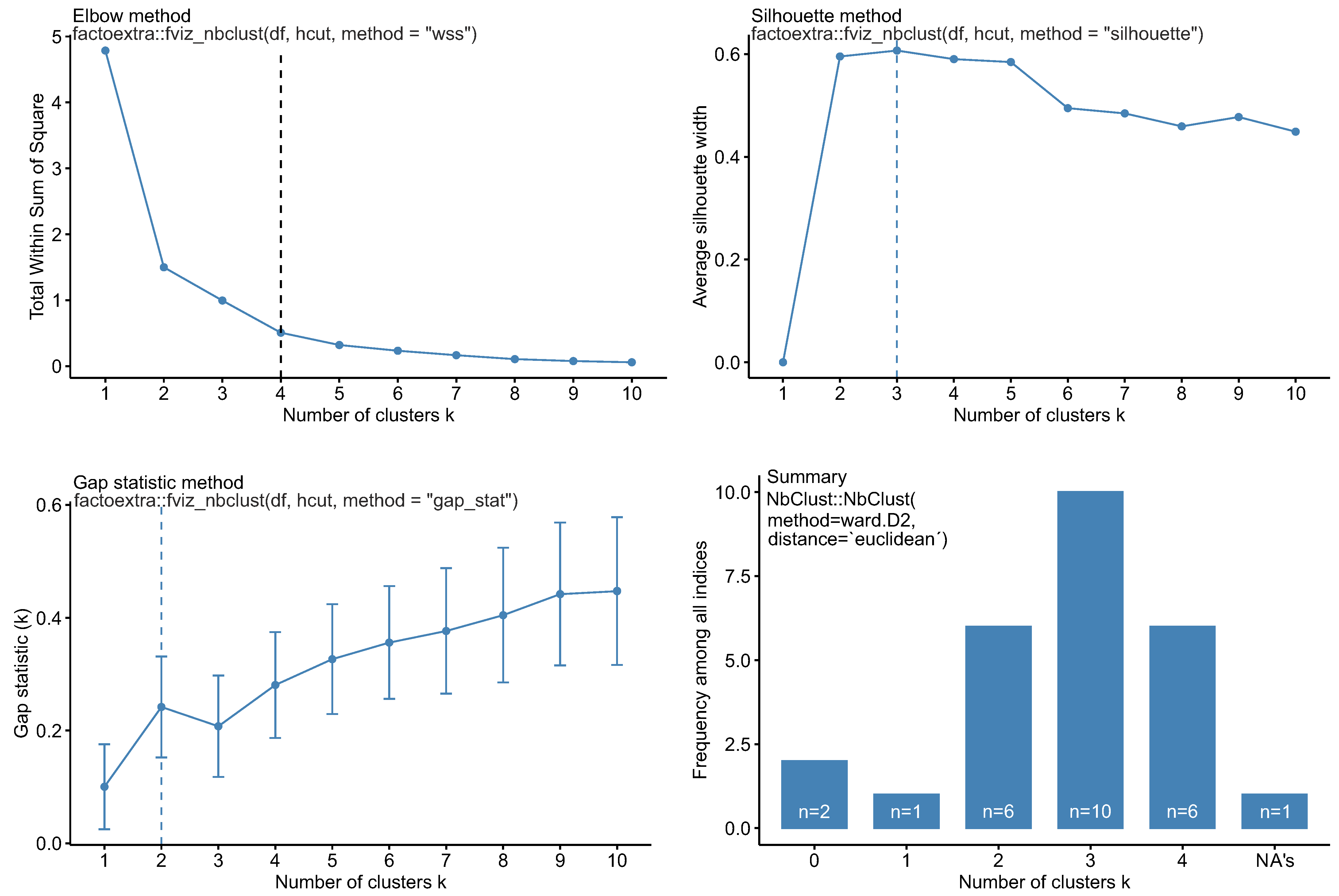
Appendix A.3. Optimal Cluster Number for HCA

Figure A1. Optimal cluster numbers applied with the “Elbow method”, “Silhouette method” and “Gap statistic” using the package factoextra [95] and computing 30 methods using NbClust [105].
Water 13 01162 g0a1
The optimal number of significant cluster for HCA is depending on the applied method and is suggested to be four (Elbow method), three (Silhouette method) or two (Gap statistic method) (Figure A1). The summary of the cumulative analysis of 30 statistical methods suggests an optimal cluster number of 3 (n = 10 methods). However, based on these results, the number of statistical significant cluster ranges from 2 (n = 6) to 4 (n = 6).

Appendix A.4. Exploratory Factor Analysis (EFA)

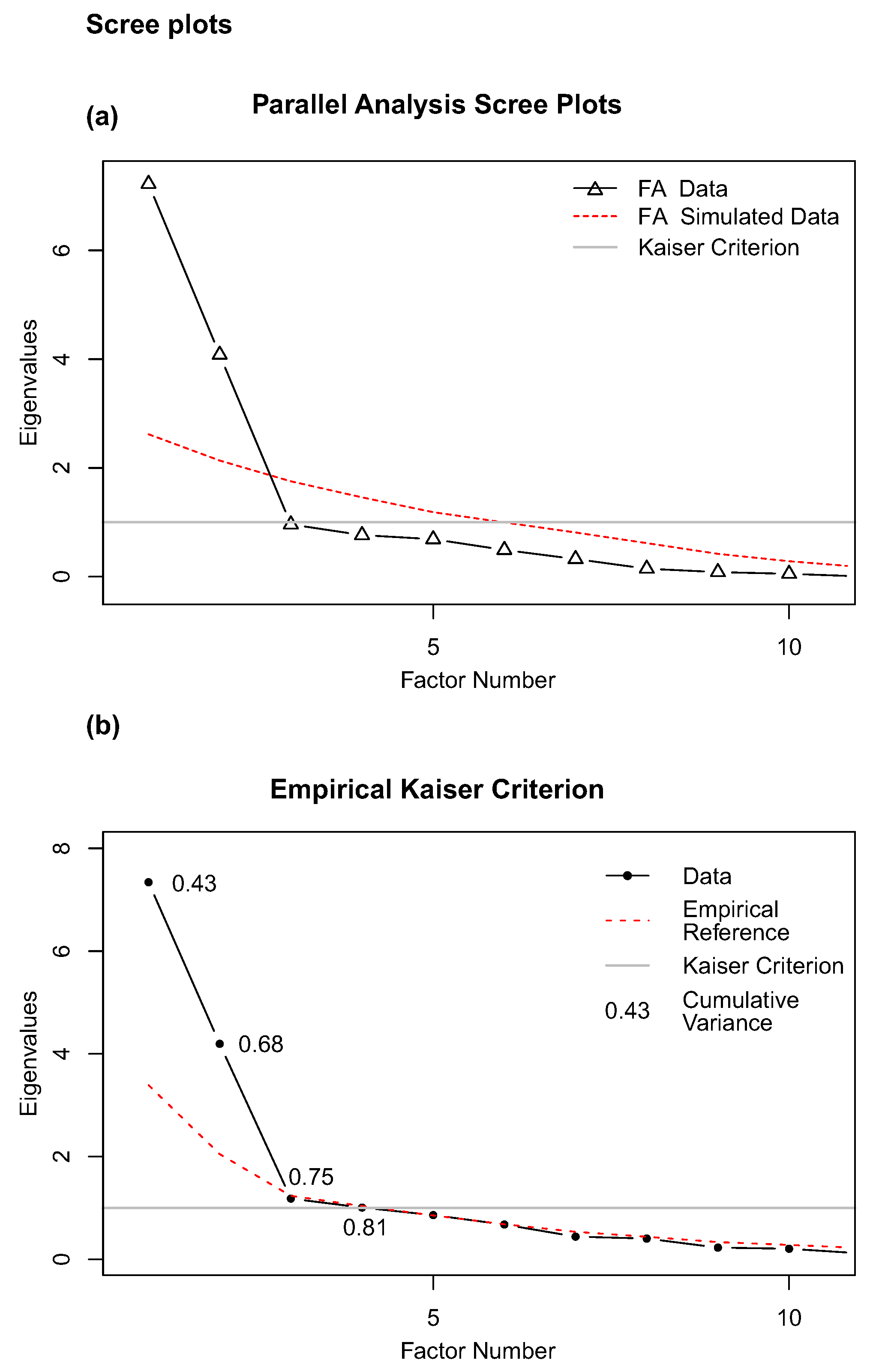
Appendix A.4.1. Determination of the Factor Number

The interpretation of parallel analysis, empirical Kaiser criterion, and Scree test resulted in a two-factor solution (Figure A2). In contrast, the Kaiser criterion (eigenvalues > 1) suggested a four-factor solution. Therefore, to increase the cumulative explained variance, a three-factor solution seems most reasonable.
The factoring method was multi-likelihood and an oblique (oblimin) rotation was performed as the variable factor loadings were not unique [96]. The loadings of the rotated three-factor solution were 4.33 for FA1, 4.61 for FA2, and 2.91 for FA3 (Table A5). The explained variance of 70 % in the data set indicates that the three factors of the 17 used variables were not capable of covering all the hydrogeological processes affecting the hydrochemical composition of the thermal groundwater in this study.
A four-factor solution indicated by the Kaiser criterion resulted in (ultra-)Heywood-cases (communalities h 2 1, an impossible outcome [111]), and was therefore declined.
Figure A2. Scree plots of (a) parallel analysis and (b) empirical Kaiser criterion with cumulative variance of the eigenvalues. Parallel analysis and empirical Kaiser criterion suggest a 2-factor solution of the EFA and Kaiser criterion suggests a 4-factor solution.
Water 13 01162 g0a2

Appendix A.4.2. Factor Loadings and Pre-Assessed Tests for Statistical Basic Requirements

Table A5. Factor loadings (>0.4) of the three-factor solution with the multi likelihood method and oblique (oblimin) rotation with communalities (h 2 ) and uniqueness (u 2 ) for each parameter as well as factor loadings and explained variance for each factor.
FA1FA2FA3h 2 u 2 MSAC- α p (SWT)
HCO 3 0.97 0.940.060.50.904.9   ×   10 6
Mg 2 + 0.96 0.920.080.70.911.3   ×   10 3
Ca 2 + 0.87 0.880.120.70.903.4   ×   10 6
EC0.75 0.910.090.70.897.0   ×   10 9
Br 0.51 0.450.550.50.906.1   ×   10 9
87 Sr/ 86 Sr0.47 0.260.740.60.911.1   ×   10 1
SO 4 2 0.92 0.940.060.90.895.0   ×   10 9
Li + 0.86 0.860.140.70.891.4   ×   10 8
F 0.71 0.360.640.70.901.7   ×   10 1
DOC 0.71 0.750.250.80.901.6   ×   10 9
SWI-dist 0.60 0.520.480.50.902.2   ×   10 8
B 0.42 0.360.640.90.903.0   ×   10 8
Sr 2 + 0.70 0.470.530.70.901.9   ×   10 7
Na + 0.930.920.080.70.892.5   ×   10 9
K + 0.660.860.140.80.895.3   ×   10 6
Cl 0.640.800.200.70.892.7   ×   10 9
Rb + −0.52 0.520.650.350.90.911.1   ×   10 3
Loadings4.334.612.91
Proportion Variance0.250.270.17
Cumulative Variance0.250.530.70
Overall KMO and C- α 0.70.90

References

  1. Goldscheider, N.; Mádl-Szőnyi, J.; Erőss, A.; Schill, E. Review: Thermal water resources in carbonate rock aquifers. Hydrogeol. J. 2010, 18, 1303–1318. [Google Scholar] [CrossRef] [Green Version]
  2. Stober, I. Hydrochemical properties of deep carbonate aquifers in the SW German Molasse basin. Geotherm. Energy 2014, 2, 13. [Google Scholar] [CrossRef] [Green Version]
  3. Bohnsack, D.; Potten, M.; Pfrang, D.; Wolpert, P.; Zosseder, K. Porosity–permeability relationship derived from Upper Jurassic carbonate rock cores to assess the regional hydraulic matrix properties of the Malm reservoir in the South German Molasse Basin. Geotherm. Energy 2020, 8, 12. [Google Scholar] [CrossRef]
  4. Konrad, F.; Savvatis, A.; Wellmann, F.; Zosseder, K. Hydraulic behavior of fault zones in pump tests of geothermal wells: A parametric analysis using numerical simulations for the Upper Jurassic aquifer of the North Alpine Foreland Basin. Geotherm. Energy 2019, 7, 25. [Google Scholar] [CrossRef]
  5. Barbieri, M.; Boschetti, T.; Petitta, M.; Tallini, M. Stable isotope (2H, 18O and 87Sr/86Sr) and hydrochemistry monitoring for groundwater hydrodynamics analysis in a karst aquifer (Gran Sasso, Central Italy). Appl. Geochem. 2005, 20, 2063–2081. [Google Scholar] [CrossRef]
  6. Zhu, G.; Li, Z.; Su, Y.; Ma, J.; Zhang, Y. Hydrogeochemical and isotope evidence of groundwater evolution and recharge in Minqin Basin, Northwest China. J. Hydrol. 2007, 333, 239–251. [Google Scholar] [CrossRef]
  7. Bouchaou, L.; Michelot, J.; Vengosh, A.; Hsissou, Y.; Qurtobi, M.; Gaye, C.; Bullen, T.; Zuppi, G. Application of multiple isotopic and geochemical tracers for investigation of recharge, salinization, and residence time of water in the Souss–Massa aquifer, southwest of Morocco. J. Hydrol. 2008, 352, 267–287. [Google Scholar] [CrossRef]
  8. Varsányi, I.; Palcsu, L.; Kovács, L.Ó. Groundwater flow system as an archive of palaeotemperature: Noble gas, radiocarbon, stable isotope and geochemical study in the Pannonian Basin, Hungary. Appl. Geochem. 2011, 26, 91–104. [Google Scholar] [CrossRef]
  9. Ettayfi, N.; Bouchaou, L.; Michelot, J.; Tagma, T.; Warner, N.; Boutaleb, S.; Massault, M.; Lgourna, Z.; Vengosh, A. Geochemical and isotopic (oxygen, hydrogen, carbon, strontium) constraints for the origin, salinity, and residence time of groundwater from a carbonate aquifer in the Western Anti-Atlas Mountains, Morocco. J. Hydrol. 2012, 438–439, 97–111. [Google Scholar] [CrossRef]
  10. Mayer, A.; Sültenfuß, J.; Travi, Y.; Rebeix, R.; Purtschert, R.; Claude, C.; Le Gal La Salle, C.; Miche, H.; Conchetto, E. A multi-tracer study of groundwater origin and transit-time in the aquifers of the Venice region (Italy). Appl. Geochem. 2014, 50, 177–198. [Google Scholar] [CrossRef]
  11. Batlle-Aguilar, J.; Banks, E.W.; Batelaan, O.; Kipfer, R.; Brennwald, M.S.; Cook, P.G. Groundwater residence time and aquifer recharge in multilayered, semi-confined and faulted aquifer systems using environmental tracers. J. Hydrol. 2017, 546, 150–165. [Google Scholar] [CrossRef]
  12. Barbieri, M. Isotopes in Hydrology and Hydrogeology. Water 2019, 11, 291. [Google Scholar] [CrossRef] [Green Version]
  13. McKay, J.; Lenczewski, M.; Leal-Bautista, R.M. Characterization of Flowpath Using Geochemistry and 87Sr/86Sr Isotope Ratios in the Yalahau Region, Yucatan Peninsula, Mexico. Water 2020, 12, 2587. [Google Scholar] [CrossRef]
  14. Wu, C.; Wu, X.; Mu, W.; Zhu, G. Using Isotopes (H, O, and Sr) and Major Ions to Identify Hydrogeochemical Characteristics of Groundwater in the Hongjiannao Lake Basin, Northwest China. Water 2020, 12, 1467. [Google Scholar] [CrossRef]
  15. Castro, M.C.; Jambon, A.; de Marsily, G.; Schlosser, P. Noble gases as natural tracers of water circulation in the Paris Basin: 1. Measurements and discussion of their origin and mechanisms of vertical transport in the basin. Water Resour. Res. 1998, 34, 2443–2466. [Google Scholar] [CrossRef]
  16. Castro, M.C.; Goblet, P.; Ledoux, E.; Violette, S.; de Marsily, G. Noble gases as natural tracers of water circulation in the Paris Basin: 2. Calibration of a groundwater flow model using noble gas isotope data. Water Resour. Res. 1998, 34, 2467–2483. [Google Scholar] [CrossRef]
  17. Millot, R.; Guerrot, C.; Innocent, C.; Négrel, P.; Sanjuan, B. Chemical, multi-isotopic (Li–B–Sr–U–H–O) and thermal characterization of Triassic formation waters from the Paris Basin. Chem. Geol. 2011, 283, 226–241. [Google Scholar] [CrossRef] [Green Version]
  18. Szocs, T.; Rman, N.; Süveges, M.; Palcsu, L.; Tóth, G.; Lapanje, A. The application of isotope and chemical analyses in managing transboundary groundwater resources. Appl. Geochem. 2013, 32, 95–107. [Google Scholar] [CrossRef]
  19. Gerber, C.; Vaikmäe, R.; Aeschbach, W.; Babre, A.; Jiang, W.; Leuenberger, M.; Lu, Z.T.; Mokrik, R.; Müller, P.; Raidla, V.; et al. Using 81Kr and noble gases to characterize and date groundwater and brines in the Baltic Artesian Basin on the one-million-year timescale. Geochim. Cosmochim. Acta 2017, 205, 187–210. [Google Scholar] [CrossRef] [Green Version]
  20. Panda, U.C.; Sundaray, S.K.; Rath, P.; Nayak, B.B.; Bhatta, D. Application of factor and cluster analysis for characterization of river and estuarine water systems—A case study: Mahanadi River (India). J. Hydrol. 2006, 331, 434–445. [Google Scholar] [CrossRef]
  21. Cloutier, V.; Lefebvre, R.; Therrien, R.; Savard, M.M. Multivariate statistical analysis of geochemical data as indicative of the hydrogeochemical evolution of groundwater in a sedimentary rock aquifer system. J. Hydrol. 2008, 353, 294–313. [Google Scholar] [CrossRef]
  22. Menció, A.; Folch, A.; Mas-Pla, J. Identifying key parameters to differentiate groundwater flow systems using multifactorial analysis. J. Hydrol. 2012, 472–473, 301–313. [Google Scholar] [CrossRef]
  23. Matiatos, I.; Alexopoulos, A.; Godelitsas, A. Multivariate statistical analysis of the hydrogeochemical and isotopic composition of the groundwater resources in northeastern Peloponnesus (Greece). Sci. Total Environ. 2014, 476–477, 577–590. [Google Scholar] [CrossRef]
  24. Lemcke, K.; Tunn, W. Tiefenwasser in der süddeutschen Molasse und ihrer verkarsteten Malmunterlage. Bull. Ver. Schweiz Pet. Geol. Ingenieure 1956, 23, 35–56. [Google Scholar]
  25. Lemcke, K. Übertiefe Grundwässer im süddeutschen Alpenvorland. Bull. Ver. Schweiz Pet. Geol. Ingenieure 1976, 42, 9–18. [Google Scholar]
  26. Udluft, P. Das tiefere Grundwasser zwischen Vindelicischem Rücken und Alpenrand. [The deeper groundwater between the Vindelician ridge and the margin of the Alps]. Geol. Jahrb. 1975, C11, 3–29. [Google Scholar]
  27. Villinger, E. Über Potentialverteilung und Strömungssysteme im Karstwasser der Schwäbischen Alb (Oberer Jura, SW-Deutschland). [On Potential Distribution and Flow Systems of the Karstwater of the Swabian Alb (Upper Jurassic, South-West-Germany)]. Geol. Jahrb. 1977, C18, 3–93. [Google Scholar]
  28. Andres, G.; Frisch, H. Hydrogeologie und Hydraulik im Malmkarst des Molassebeckens und der angrenzenden Fränkisch-Schwäbischen Alb. In Die Thermal- und Schwefelwasservorkommen von Bad Gögging; Andres, G., Wirth, H., Eds.; Schriftenreihe Bayerisches Landesamt für Wasserwirtschaft: München, Germany, 1981; Volume 15, Chapter 11; pp. 108–117. [Google Scholar]
  29. Stichler, W.; Rauert, W.; Weise, S.; Wolf, M.; Koschel, G.; Stier, P.; Prestel, R.; Hedin, K.; Bertleff, B. Isotopenhydrologische und hydrochemische Untersuchungen zur Erkundung des Fließsystems im Malmkarstaquifer des süddeutschen Alpenvorlandes. [Isotope-hydrological and Hydrochemical Investigations of the Flow System of the Malmkarst Aquifer in the Pre-Alpine Region of South Germany]. Zeitschrift der Deutschen Geologischen Gesellschaft 1987, 138, 387–398. [Google Scholar]
  30. Villinger, E. Bemerkungen zur Verkarstung des Malms unter dem westlichen süddeutschen Molassebecken. [Comments on the karstification of the Malm under the western molasse basin in South Germany]. Bull. Ver. Schweiz Pet. Geol. Ingenieure 1988, 54, 41–59. [Google Scholar] [CrossRef]
  31. Balderer, W. Hydrogeologische Charakterisierung der Grundwasservorkommen innerhalb der Molasse der Nordostschweiz aufgrund von hydrochemischen und Isotopenuntersuchungen. [Hydrogeological Characterization of the Groundwater Reservoirs in the Molasse of the North-East of Switzerland on the Basis of Hydrochemical Investigations and Isotope Methods]. Steirische BeiträGe Hydrogeol. 1990, 41, 35–104. [Google Scholar]
  32. Bertleff, B.; Ellwanger, D.; Szenkler, C.; Eichinger, L.; Trimborn, P.; Wolfendale, N. Interpretation of hydrochemical and hydroisotopical measurements on palaeogroundwaters in Oberschwaben, South German Alpine foreland, with focus on quaternary geology. In International Symposium on Applications of Isotope Techniques in Studying Past and Current Environmental Changes in the Hydrosphere and the Atmosphere; International Atomic Energy Agency (IAEA): Vienna, Austria, 1993; Volume IAEA-SM-329/66, pp. 337–357. [Google Scholar]
  33. Stichler, W. Isotopengehalte in Tiefengrundwässern aus Erdöl- und Erdgasbohrungen im süddeutschen Molassebecken. [Isotope contents of deep groundwater from oil and gas wells located in the South German Molasse basin]. Beiträge Hydrogeol. 1997, 48, 81–88. [Google Scholar]
  34. Prestel, R. Hydrochemische Untersuchungen im süddeutschen Molassebecken. In Schlussbericht Forschungsvorhaben 03 E 6240 A/B: Hydrogeothermische Energiebilanz und Grundwasserhaushalt des Malmkarstes im süddeutschen Molassebecken, 1991; Frisch, H., Werner, J., Eds.; Bayerisches Landesamt für Wasserwirtschaft, Geologisches Landesamt Baden-Württemberg: München, Freiburg i. Br., Germany, 1988; Chapter 4; p. 64. [Google Scholar]
  35. Weise, S.; Wolf, M.; Fritz, P.; Rauert, W.; Stichler, W.; Prestel, R.; Bertleff, B.; Stute, M. Isotopenhydrologische Untersuchungen im Süddeutschen Molassebecken. In Schlussbericht Forschungsvorhaben 03 E 6240 A/B: Hydrogeothermische Energiebilanz und Grundwasserhaushalt des Malmkarstes im süddeutschen Molassebecken, 1991; Frisch, H., Werner, J., Eds.; Bayerisches Landesamt für Wasserwirtschaft, Geologisches Landesamt Baden-Württemberg: München, Freiburg i. Br., Germany, 1991; Chapter 5; p. 106. [Google Scholar]
  36. Frisch, H.; Huber, B. Ein hydrogeologisches Modell und der Versuch einer Bilanzierung des Thermalwasservorkommens im Malmkarst des süddeutschen Molassebeckens. [A Hydrogeological Model and the Attempt of a Balance of the Thermal Water for the Malmkarst in the Southgerman and the Neighbouring Upper Austrian Molasse Basin]. Hydrogeol. Umw. 2000, 20, 25–43. [Google Scholar]
  37. Birner, J.; Mayr, C.; Thomas, L.; Schneider, M.; Baumann, T.; Winkler, A. Hydrochemie und Genese der tiefen Grundwässer des Malmaquifers im bayerischen Teil des süddeutschen Molassebeckens. [Hydrochemistry and evolution of deep groundwaters in the Malm aquifer in the bavarian part of the South German Molasse Basin]. Z. Geol. Wiss. 2011, 39, 291–308. [Google Scholar]
  38. Mayrhofer, C.; Niessner, R.; Baumann, T. Hydrochemistry and hydrogen sulfide generating processes in the Malm aquifer, Bavarian Molasse Basin, Germany. Hydrogeol. J. 2014, 22, 151–162. [Google Scholar] [CrossRef]
  39. Savvatis, A.; Steiner, U.; Huber, B.; Fritzer, T.; Schneider, M. Limitierungen bei der Ermittlung der Grundwasserfließrichtung in tiefen Aquiferen am Beispiel des Malms im Süddeutschen Molassebecken. [Limitations in the identification of the groundwater flow direction in deep aquifers using the example of the Malm in the Southern German Molasse Basin]. Grundwasser 2015, 20, 271–280. [Google Scholar] [CrossRef]
  40. Mraz, E.; Wolfgramm, M.; Moeck, I.; Thuro, K. Detailed Fluid Inclusion and Stable Isotope Analysis on Deep Carbonates from the North Alpine Foreland Basin to Constrain Paleofluid Evolution. Geofluids 2019, 2019, 1–23. [Google Scholar] [CrossRef] [Green Version]
  41. Birner, J.; Fritzer, T.; Jodocy, M.; Savvatis, A.; Schneider, M.; Stober, I. Hydraulische Eigenschaften des Malmaquifers im Süddeutschen Molassebecken und ihre Bedeutung für die geothermische Erschließung. [Hydraulic characterisation of the Malm aquifer in the South German Molasse basin and its impact on geothermal exploitations]. Z. Geol. Wiss. 2012, 40, 133–156. [Google Scholar]
  42. Wanner, C.; Eichinger, F.; Jahrfeld, T.; Diamond, L.W. Unraveling the Formation of Large Amounts of Calcite Scaling in Geothermal Wells in the Bavarian Molasse Basin: A Reactive Transport Modeling Approach. Procedia Earth Planet. Sci. 2017, 17, 344–347. [Google Scholar] [CrossRef] [Green Version]
  43. Köhl, B.; Grundy, J.; Baumann, T. Rippled scales in a geothermal facility in the Bavarian Molasse Basin: A key to understand the calcite scaling process. Geotherm. Energy 2020, 8, 23. [Google Scholar] [CrossRef]
  44. Heidinger, M.; Eichinger, F.; Purtschert, R.; Mueller, P.; Zappala, J.; Wirsing, G.; Geyer, T.; Fritzer, T.; Groß, D. Altersbestimmung an thermalen Tiefenwässern im Oberjura des Molassebeckens mittels Krypton-Isotopen. [81Kr/85Kr-Dating of thermal groundwaters in the Upper Jurassic (Molasse Basin)]. Grundwasser 2019, 24, 287–294. [Google Scholar] [CrossRef] [Green Version]
  45. Bachmann, G.; Müller, M.; Weggen, K. Evolution of the Molasse Basin (Germany, Switzerland). Tectonophysics 1987, 137, 77–92. [Google Scholar] [CrossRef]
  46. Freudenberger, W.; Schwerd, K. Erläuterungen zur Geologischen Karte von Bayern 1:500000, 4th ed.; Bayerisches Geologisches Landesamt: Munich, Germany, 1996; p. 329. [Google Scholar]
  47. Doppler, G.; Heissig, K.; Reichenbacher, B. Die Gliederung des Tertiars im sueddeutschen Molassebecken. Newsl. Stratigr. 2006, 41, 359–375. [Google Scholar] [CrossRef]
  48. Lemcke, K. Geologie von Bayern I.-Das bayerische Alpenvorland vor der Eiszeit-Erdgeschichte-Bau-Bodenschätze; Schweizerbart: Stuttgart, Germany, 1988; p. 175. [Google Scholar]
  49. Drews, M.C.; Seithel, R.; Savvatis, A.; Kohl, T.; Stollhofen, H. A normal-faulting stress regime in the Bavarian Foreland Molasse Basin? New evidence from detailed analysis of leak-off and formation integrity tests in the greater Munich area, SE-Germany. Tectonophysics 2019, 755, 1–9. [Google Scholar] [CrossRef]
  50. Agemar, T.; Alten, J.A.; Ganz, B.; Kuder, J.; Kühne, K.; Schumacher, S.; Schulz, R. The Geothermal Information System for Germany—GeotIS. Z. der Dtsch. Ges. für Geowiss. 2014, 165, 129–144. [Google Scholar] [CrossRef]
  51. Agemar, T.; Weber, J.; Schulz, R. Deep Geothermal Energy Production in Germany. Energies 2014, 7, 4397–4416. [Google Scholar] [CrossRef]
  52. Böhm, F.; Savvatis, A.; Steiner, U.; Schneider, M.; Koch, R. Lithofazielle Reservoircharakterisierung zur geothermischen Nutzung des Malm im Großraum München. [Lithofacies and characterization of the geothermal Malm reservoir in the greater area of Munich]. Grundwasser 2013, 18, 3–13. [Google Scholar] [CrossRef]
  53. Konrad, F.; Savvatis, A.; Degen, D.; Wellmann, F.; Einsiedl, F.; Zosseder, K. Productivity enhancement of geothermal wells through fault zones: Efficient numerical evaluation of a parameter space for the Upper Jurassic aquifer of the North Alpine Foreland Basin. Geothermics 2021. (accepted). [Google Scholar]
  54. Furtak, H.; Langguth, H. Zur hydrochemischen Kennzeichnung von Grundwässern und Grundwassertypen mittels Kennzahlen. Mem. IAH-Congr. 1967, VII, 86–96. [Google Scholar]
  55. Hahn-Weihnheimer, P.; Hirner, A.; Lemcke, K. Zur Herkunft süddeutscher Erdöle—Geochemische Ergebnisse und Versuch einer geologischen Interpretation. [On the origin of crude oils from Southern Germany—Geochemical results and a tentative geological interpretation]. Bull. Der Ver. Schweiz Pet. Geol. Ingenieure 1979, 45, 35–46. [Google Scholar] [CrossRef]
  56. Stober, I.; Wolfgramm, M.; Birner, J. Hydrochemie der Tiefenwässer in Deutschland. [Hydrochemistry of deep waters in Germany]. Z. Geol. Wiss. 2014, 41/42, 339–380. [Google Scholar]
  57. Bertleff, B.; Watzel, R. Tiefe Aquifersysteme im südwestdeutschen Molassebecken. Eine umfassende hydrogeologische Analyse als Grundlage eines zukünftigen Quantitäts- und Qualitätsmanagements. [Deep Aquifer Systems in the Southwest German Molasse basin. An extensive hydro-geological analysis as the basis for future quantitative and qualitative groundwater management]. Abh. Geol. Landesamt Baden Württemberg 2002, 15, 75–90. [Google Scholar]
  58. Heine, F.; Einsiedl, F. Groundwater dating with dissolved organic radiocarbon: A promising approach in carbonate aquifers. Appl. Geochem. 2021, 125. [Google Scholar] [CrossRef]
  59. Dehnert, J.; Nestler, W.; Freyer, K.; Treutler, H.; Neitzel, P.L.; Walther, W. Bestimmung der notwendigen Abpumpzeiten von Grundwasserbeobachtungsrohren mit Hilfe der natürlichen Radonaktivitätskonzentration. In Grundwasser und Rohstoffgewinnung. GeoCongress 2; Merkel, B., Dietrich, P.G., Struckmeier, W., Löhnert, E.P., Eds.; 1996; pp. 40–45. Available online: https://www.researchgate.net/publication/313730398_Bestimmung_der_notwendigen_Abpumpzeiten_von_Grundwasserbeobachtungsrohren_mit_Hilfe_der_naturlichen_Radonaktivitatskonzentration (accessed on 20 April 2021).
  60. Craig, H. Isotopic Variations in Meteoric Waters. Science 1961, 133, 1702–1703. [Google Scholar] [CrossRef] [PubMed]
  61. Kharaka, Y.; Hanor, J. Deep Fluids in Sedimentary Basins. In Treatise on Geochemistry; Holland, H., Turekian, K., Eds.; Elsevier Science: Amsterdam, The Netherlands, 2014; Volume 7, pp. 471–515. [Google Scholar] [CrossRef]
  62. Stumpp, C.; Klaus, J.; Stichler, W. Analysis of long-term stable isotopic composition in German precipitation. J. Hydrol. 2014, 517, 351–361. [Google Scholar] [CrossRef]
  63. Rosner, M. Geochemical and instrumental fundamentals for accurate and precise strontium isotope data of food samples: Comment on “Determination of the strontium isotope ratio by ICP-MS ginseng as a tracer of regional origin” (Choi et al., 2008). Food Chem. 2010, 121, 918–921. [Google Scholar] [CrossRef]
  64. Sültenfuß, J.; Roether, W.; Rhein, M. The Bremen mass spectrometric facility for the measurement of helium isotopes, neon, and tritium in water. Isot. Environ. Health Stud. 2009, 45, 83–95. [Google Scholar] [CrossRef] [PubMed]
  65. Aeschbach-Hertig, W.; Solomon, D.K. Noble Gas Thermometry in Groundwater Hydrology. In The Noble Gases as Geochemical Tracers; Burnard, P., Ed.; Advances in Isotope Geochemistry; Springer: Berlin/Heidelberg, Germany, 2013; pp. 81–122. [Google Scholar] [CrossRef]
  66. Andrews, J.N.; Lee, D.J. Inert gases in groundwater from the Bunter Sandstone of England as indicators of age and palaeoclimatic trends. J. Hydrol. 1979, 41, 233–252. [Google Scholar] [CrossRef]
  67. Andrews, J.; Goldbrunner, J.; Darling, W.; Hooker, P.; Wilson, G.; Youngman, M.; Eichinger, L.; Rauert, W.; Stichler, W. A radiochemical, hydrochemical and dissolved gas study of groundwaters in the Molasse basin of Upper Austria. Earth Planet. Sci. Lett. 1985, 73, 317–332. [Google Scholar] [CrossRef]
  68. Aeschbach-Hertig, W.; Peeters, F.; Beyerle, U.; Kipfer, R. Palaeotemperature reconstruction from noble gases in ground water taking into account equilibration with entrapped air. Nature 2000, 405, 1040–1044. [Google Scholar] [CrossRef] [Green Version]
  69. Kipfer, R.; Aeschbach-Hertig, W.; Peeters, F.; Stute, M. Noble Gases in Lakes and Ground Waters. In Noble Gases; Porcelli, D.P., Ballentine, C.J., Wieler, R., Eds.; De Gruyter: Berlin, Germany; Boston, MA, USA, 2002; Volume 47, Chapter 14; pp. 615–700. [Google Scholar] [CrossRef] [Green Version]
  70. Stute, M.; Schlosser, P. Principles and Applications of the Noble Gas Paleothermometer. In Climate Change in Continental Isotopic Records; Swart, P., Lohmann, K.C., McKenzie, J., Savin, S., Eds.; AGU: Washington, DC, USA, 1993; pp. 89–100. [Google Scholar] [CrossRef]
  71. Wilson, G.; McNeill, G. Noble gas recharge temperatures and the excess air component. Appl. Geochem. 1997, 12, 747–762. [Google Scholar] [CrossRef]
  72. Jung, M.; Aeschbach, W. A new software tool for the analysis of noble gas data sets from (ground)water. Environ. Model. Softw. 2018, 103, 120–130. [Google Scholar] [CrossRef]
  73. Jung, M.; Wieser, M.; von Oehsen, A.; Aeschbach-Hertig, W. Properties of the closed-system equilibration model for dissolved noble gases in groundwater. Chem. Geol. 2013, 339, 291–300. [Google Scholar] [CrossRef]
  74. Kulongoski, J.; Hilton, D. Applications of Groundwater Helium. In Handbook of Environmental Isotope Geochemistry; Advances in Isotope Geochemistry; Baskaran, M., Ed.; Springer: Berlin/Heidelberg, Germany, 2012; Chapter 15; pp. 285–304. [Google Scholar] [CrossRef]
  75. Bethke, C.M.; Johnson, T.M. Paradox of groundwater age. Geology 2002, 30, 107–110. [Google Scholar] [CrossRef]
  76. Tolstikhin, I.; Lehmann, B.; Loosli, H.; Gautschi, A. Helium and argon isotopes in rocks, minerals, and related ground waters: A case study in northern Switzerland. Geochim. Cosmochim. Acta 1996, 60, 1497–1514. [Google Scholar] [CrossRef]
  77. Kulongoski, J.T.; Hilton, D.R.; Izbicki, J.A. Helium isotope studies in the Mojave Desert, California: Implications for groundwater chronology and regional seismicity. Chem. Geol. 2003, 202, 95–113. [Google Scholar] [CrossRef]
  78. Clarke, W.; Jenkins, W.; Top, Z. Determination of tritium by mass spectrometric measurement of 3He. Int. J. Appl. Radiat. Isot. 1976, 27, 515–522. [Google Scholar] [CrossRef]
  79. Ballentine, C.J.; Burnard, P.G. Production, Release and Transport of Noble Gases in the Continental Crust. Rev. Mineral. Geochem. 2002, 47, 481–538. [Google Scholar] [CrossRef]
  80. Phillips, F.; Castro, M. Groundwater Dating and Residence-Time Measurements. In Treatise on Geochemistry; Holland, H., Turekian, K., Eds.; Elsevier Science: Amsterdam, The Netherlands, 2014; Volume 7, pp. 361–400. [Google Scholar] [CrossRef]
  81. Graham, D.W. Noble Gas Isotope Geochemistry of Mid-Ocean Ridge and Ocean Island Basalts: Characterization of Mantle Source Reservoirs. Rev. Mineral. Geochem. 2002, 47, 247–317. [Google Scholar] [CrossRef]
  82. Lippmann, J.; Stute, M.; Torgersen, T.; Moser, D.; Hall, J.; Lin, L.; Borcsik, M.; Bellamy, R.; Onstott, T. Dating ultra-deep mine waters with noble gases and 36Cl, Witwatersrand Basin, South Africa. Geochim. Cosmochim. Acta 2003, 67, 4597–4619. [Google Scholar] [CrossRef]
  83. Ozima, M.; Podosek, F.A. Noble Gas Geochemistry; Cambridge University Press: Cambridge, UK, 2002; p. 286. [Google Scholar]
  84. Lee, J.Y.; Marti, K.; Severinghaus, J.P.; Kawamura, K.; Yoo, H.S.; Lee, J.B.; Kim, J.S. A redetermination of the isotopic abundances of atmospheric Ar. Geochim. Cosmochim. Acta 2006, 70, 4507–4512. [Google Scholar] [CrossRef]
  85. Andrews, J.N.; Youngman, M.J.; Goldbrunner, J.E.; Darling, W.G. The geochemistry of formation waters in the molasse basin of upper Austria. Environ. Geol. Water Sci. 1987, 10, 43–57. [Google Scholar] [CrossRef]
  86. Weise, S.; Moser, H. Groundwater dating with helium isotopes. In International Symposium on the Use of Isotope Techniques in Water Resources Development, 1987; International Atomic Energy Agency (IAEA): Vienna, Austria, 1987; Volume IAEA-SM-299/44, pp. 105–126. [Google Scholar]
  87. Osenbrück, K.; Lippmann, J.; Sonntag, C. Dating very old pore waters in impermeable rocks by noble gas isotopes. Geochim. Cosmochim. Acta 1998, 62, 3041–3045. [Google Scholar] [CrossRef]
  88. Torgersen, T.; Stute, M. Helium (and other noble gases) as a tool for understanding long time-scale groundwater transport. In Isotope Methods for Dating Old Groundwater; International Atomic Energy Agency (IAEA): Vienna, Austria, 2013; Chapter 8; pp. 179–244. [Google Scholar]
  89. Petersen, J.; Deschamps, P.; Hamelin, B.; Fourré, E.; Gonçalvès, J.; Zouari, K.; Guendouz, A.; Michelot, J.L.; Massault, M.; Dapoigny, A.; et al. Groundwater flowpaths and residence times inferred by 14C, 36Cl and 4He isotopes in the Continental Intercalaire aquifer (North-Western Africa). J. Hydrol. 2018, 560, 11–23. [Google Scholar] [CrossRef]
  90. Weiss, R.F. Solubility of helium and neon in water and seawater. J. Chem. Eng. Data 1971, 16, 235–241. [Google Scholar] [CrossRef]
  91. Stute, M.; Sonntag, C.; Deák, J.; Schlosser, P. Helium in deep circulating groundwater in the Great Hungarian Plain: Flow dynamics and crustal and mantle helium fluxes. Geochim. Cosmochim. Acta 1992, 56, 2051–2067. [Google Scholar] [CrossRef]
  92. Torgersen, T.; Clarke, W.B. Helium accumulation in groundwater, I: An evaluation of sources and the continental flux of crustal 4He in the Great Artesian Basin, Australia. Geochim. Cosmochim. Acta 1985, 49, 1211–1218. [Google Scholar] [CrossRef]
  93. Thuro, K.; Zosseder, K.; Bohnsack, D.; Heine, F.; Konrad, F.; Mraz, E.; Stockinger, G. Dolomitkluft: Erschließung, Test und Analyse des ersten kluftdominierten Dolomitaquifers im tiefen Malm des Molassebeckens zur Erhöhung der Erfolgsaussichten; Technical Report; Technical University of Munich: Munich, Germany, 2019. [Google Scholar]
  94. Belkhiri, L.; Boudoukha, A.; Mouni, L.; Baouz, T. Application of multivariate statistical methods and inverse geochemical modeling for characterization of groundwater—A case study: Ain Azel plain (Algeria). Geoderma 2010, 159, 390–398. [Google Scholar] [CrossRef]
  95. Kassambara, A. Practical Guide to Cluster Analysis in R, 1st ed.; 2017; p. 187. Available online: https://www.datanovia.com/en/product/practical-guide-to-cluster-analysis-in-r/ (accessed on 21 April 2021).
  96. Schumacker, R.E. Using R with Multivariate Statistics; SAGE Publications: Los Angeles, CA, USA, 2016; p. 408. [Google Scholar]
  97. Tabachnik, B.G.; Fidell, L.S. Using Multivariate Statistics, 6th ed.; Pearson: New York, NY, USA, 2013; p. 983. [Google Scholar]
  98. R Core Team. R: A Language and Environment for Statistical Computing; R Foundation for Statistical Computing: Vienna, Austria, 2020. [Google Scholar]
  99. Revelle, W. psych: Procedures for Psychological, Psychometric, and Personality Research; Northwestern University: Evanston, IL, USA, 2019. [Google Scholar]
  100. Jorgensen, T.D.; Pornprasertmanit, S.; Schoemann, A.M.; Rosseel, Y. semTools: Useful Tools for Structural Equation Modeling; 2000. Available online: https://CRAN.R-project.org/package=semTools (accessed on 21 April 2021).
  101. Wickham, H. Elegant Graphics for Data Analysis: Ggplot2; Springer: New York, NY, USA, 2008; pp. 21–54. [Google Scholar] [CrossRef]
  102. Backhaus, K.; Erichson, B.; Plinke, W.; Weiber, R. Multivariate Analysemethoden; Springer: Berlin/Heidelberg, Germany, 2016; Volume 14, p. 854. [Google Scholar] [CrossRef]
  103. DiStefano, C.; Zhu, M.; Mîndrilă, D. Understanding and Using Factor Scores: Considerations for the Applied Researcher. Pract. Assess. Res. Eval. 2009, 14, 1–11. [Google Scholar] [CrossRef]
  104. Ward, J.H. Hierarchical Grouping to Optimize an Objective Function. J. Am. Stat. Assoc. 1963, 58, 236–244. [Google Scholar] [CrossRef]
  105. Charrad, M.; Ghazzali, N.; Boiteau, V.; Niknafs, A. NbClust: An R Package for Determining the Relevant Number of Clusters in a Data Set. J. Stat. Softw. 2014, 61. [Google Scholar] [CrossRef] [Green Version]
  106. Horn, J.L. A rationale and test for the number of factors in factor analysis. Psychometrika 1965, 30, 179–185. [Google Scholar] [CrossRef]
  107. Kaiser, H.F. The Application of Electronic Computers to Factor Analysis. Educ. Psychol. Meas. 1960, 20, 141–151. [Google Scholar] [CrossRef]
  108. Braeken, J.; van Assen, M.A.L.M. An empirical Kaiser criterion. Psychol. Methods 2017, 22, 450–466. [Google Scholar] [CrossRef] [Green Version]
  109. Cattell, R.B. The Scree Test for the Number of Factors. Multivar. Behav. Res. 1966, 1, 245–276. [Google Scholar] [CrossRef]
  110. Zwick, W.R.; Velicer, W.F. Factors Influencing Four Rules for Determining the Number of Components to Retain. Psychol. Bull. 1986, 99, 432–442. [Google Scholar] [CrossRef]
  111. Costello, A.B.; Osborne, J.W. Best practices in exploratory factor analysis: Four recommendations for getting the most from your analysis. Pract. Assess. Res. Eval. 2005, 10, 9. [Google Scholar]
  112. Faure, G.; Powell, J.L. Strontium Isotope Geology. In Minerals, Rocks and Inorganic Materials; Von Engelhardt, W., Hahn, T., Roy, R., Wyllie, P., Eds.; Springer: Berlin/Heidelberg, Germany; New York, NY, USA, 1972; Chapter 5; p. 188. [Google Scholar] [CrossRef]
  113. Whittemore, D.O. Geochemical differentiation of oil and gas brine from other saltwalter sources contaminating water resources: Case studies from Kansas and Oklahoma. Environ. Geosci. 1995, 2, 15–31. [Google Scholar]
  114. Collins, A.G. Geochemistry of Oilfield Waters, 1st ed.; Elsevier: Amsterdam, The Netherlands; Oxford, UK; New York, NY, USA, 1975; p. 496. [Google Scholar]
  115. Stober, I.; Bucher, K. Herkunft der Salinität in Tiefenwässern des Grundgebirges—Unter besonderer Berücksichtigung der Kristallinwässer des Schwarzwaldes. Grundwasser 2000, 3, 125–140. [Google Scholar] [CrossRef]
  116. Gemici, Ü.; Tarcan, G. Distribution of boron in thermal waters of western Anatolia, Turkey, and examples of their environmental impacts. Environ. Geol. 2002, 43, 87–98. [Google Scholar] [CrossRef]
  117. Clark, I. Groundwater Geochemistry and Isotopes; CRC Press Taylore & Francis Group: Boca Raton, FL, USA; London, UK; New York, NY, USA, 2015; p. 421. [Google Scholar]
  118. Langmuir, D. The geochemistry of some carbonate ground waters in central Pennsylvania. Geochim. Cosmochim. Acta 1971, 35, 1023–1045. [Google Scholar] [CrossRef]
  119. Mayo, A.L.; Loucks, M.D. Solute and isotopic geochemistry and ground water flow in the central Wasatch Range, Utah. J. Hydrol. 1995, 172, 31–59. [Google Scholar] [CrossRef]
  120. Clayton, R.N.; Friedman, I.; Graf, D.L.; Mayeda, T.K.; Meents, W.F.; Shimp, N.F. The origin of saline formation waters: 1. Isotopic composition. J. Geophys. Res. 1966, 71, 3869–3882. [Google Scholar] [CrossRef]
  121. Bottomley, D.J.; Conrad Gregoire, D.; Raven, K.G. Saline ground waters and brines in the Canadian Shield: Geochemical and isotopic evidence for a residual evaporite brine component. Geochim. Cosmochim. Acta 1994, 58, 1483–1498. [Google Scholar] [CrossRef]
  122. Van Geldern, R.; Baier, A.; Subert, H.L.; Kowol, S.; Balk, L.; Barth, J.A. Pleistocene paleo-groundwater as a pristine fresh water resource in southern Germany—Evidence from stable and radiogenic isotopes. Sci. Total Environ. 2014, 496, 107–115. [Google Scholar] [CrossRef] [PubMed]
  123. Weise, S.; Stichler, W. Edelgasisotopen-Methoden als Werkzeug zur Untersuchung tiefreichender Grundwasser-Fließsysteme am Beispiel des süddeutschen Molassebeckens. [Noble gas isotope methods as a tool for investigations of deep circulating groundwater flowsystems in the South German Molasse basin]. Beitr. Hydrogeol. 1997, 48, 69–80. [Google Scholar]
  124. Goldbrunner, J.E. Zum Stand der geothermischen und balneologischen Tiefengrundwassernutzung im Oststeirischen Becken und im Oberösterreichischen Molassebecken. [The Status of Geothermic and Balneologic Utilization of Deep Groundwater in the East Styrian Basin and the Upper Austrian Molasse Basin]. Z. Dtsch. Geol. Ges. 1987, 138, 513–526. [Google Scholar]
  125. Capo, R.C.; Stewart, B.W.; Chadwick, O.A. Strontium isotopes as tracers of ecosystem processes: Theory and methods. Geoderma 1998, 82, 197–225. [Google Scholar] [CrossRef]
  126. Probst, A.; El Gh’mari, A.; Aubert, D.; Fritz, B.; McNutt, R. Strontium as a tracer of weathering processes in a silicate catchment polluted by acid atmospheric inputs, Strengbach, France. Chem. Geol. 2000, 170, 203–219. [Google Scholar] [CrossRef] [Green Version]
  127. Shand, P.; Darbyshire, D.; Love, A.; Edmunds, W. Sr isotopes in natural waters: Applications to source characterisation and water–rock interaction in contrasting landscapes. Appl. Geochem. 2009, 24, 574–586. [Google Scholar] [CrossRef]
  128. Baublys, K.A.; Hamilton, S.K.; Hofmann, H.; Golding, S.D. A strontium (87Sr/86Sr) isotopic study on the chemical evolution and migration of groundwaters in a low-rank coal seam gas reservoir (Surat Basin, Australia). Appl. Geochem. 2019, 101, 1–18. [Google Scholar] [CrossRef]
  129. Veizer, J.; Ala, D.; Azmy, K.; Bruckschen, P.; Buhl, D.; Bruhn, F.; Carden, G.; Diener, A.; Ebneth, S.; Godderis, Y.; et al. 87Sr/86Sr, 13C and 18O evolution of Phanerozoic seawater. Chem. Geol. 1999, 161, 59–88. [Google Scholar] [CrossRef] [Green Version]
  130. Chaudhuri, S.; Broedel, V.; Clauer, N. Strontium isotopic evolution of oil-field waters from carbonate reservoir rocks in Bindley field, central Kansas, U.S.A. Geochim. Cosmochim. Acta 1987, 51, 45–53. [Google Scholar] [CrossRef]
  131. Heaton, T.; Vogel, J. “Excess air” in groundwater. J. Hydrol. 1981, 50, 201–216. [Google Scholar] [CrossRef]
  132. Peeters, F.; Beyerle, U.; Aeschbach-Hertig, W.; Holocher, J.; Brennwald, M.S.; Kipfer, R. Improving noble gas based paleoclimate reconstruction and groundwater dating using 20Ne/22Ne ratios. Geochim. Cosmochim. Acta 2003, 67, 587–600. [Google Scholar] [CrossRef] [Green Version]
  133. Blaser, P.; Coetsiers, M.; Aeschbach-Hertig, W.; Kipfer, R.; Van Camp, M.; Loosli, H.; Walraevens, K. A new groundwater radiocarbon correction approach accounting for palaeoclimate conditions during recharge and hydrochemical evolution: The Ledo-Paniselian Aquifer, Belgium. Appl. Geochem. 2010, 25, 437–455. [Google Scholar] [CrossRef]
  134. Lippmann, J.; Erzinger, J.; Zimmer, M.; Schloemer, S.; Eichinger, L.; Faber, E. On the geochemistry of gases and noble gas isotopes (including 222Rn) in deep crustal fluids: The 4000 m KTB-pilot hole fluid production test 2002-03. Geofluids 2005, 5, 52–66. [Google Scholar] [CrossRef]
  135. Nakata, K.; Hasegawa, T.; Solomon, D.; Miyakawa, K.; Tomioka, Y.; Ohta, T.; Matsumoto, T.; Hama, K.; Iwatsuki, T.; Ono, M.; et al. Degassing behavior of noble gases from groundwater during groundwater sampling. Appl. Geochem. 2019, 104, 60–70. [Google Scholar] [CrossRef]
  136. Sano, Y.; Fischer, T.P. The Analysis and Interpretation of Noble Gases in Modern Hydrothermal Systems. In The Noble Gases as Geochemical Tracers; Burnard, P., Ed.; Advances in Isotope Geochemistry; Springer: Berlin/Heidelberg, Germany, 2013; pp. 249–317. [Google Scholar] [CrossRef]
  137. Wasserburg, G.; Mazor, E.; Zartman, R. Isotopic and chemical composition of some terrestrial natural gases. In Earth Science and Meteorites; Geiss, J., Goldberg, E., Eds.; North-Holland Pub. Co.: Amsterdam, NL, USA, 1963; pp. 219–240. [Google Scholar]
  138. Torgersen, T.; Kennedy, B.; Hiyagon, H.; Chiou, K.; Reynolds, J.; Clarke, W. Argon accumulation and the crustal degassing flux of40Ar in the Great Artesian Basin, Australia. Earth Planet. Sci. Lett. 1989, 92, 43–56. [Google Scholar] [CrossRef]
  139. Goldbrunner, J. Hydrogeology of Deep Groundwaters in Austria. Mitteilungen Osterreichischen Geol. Ges. 1999, 92, 281–294. [Google Scholar]
Figure 2. Dendrogram plots of hierarchical cluster analysis (HCA) (n = 24, m = 17) in two steps resulting in four clusters (C1-1 to C2-1) and outliers. (a) step 1 using single linkage method for outlier detection of observations with the greatest distance in the data set. (b) Step 2 using Ward’s method to find clusters C1-1 to C2-1.
Water 13 01162 g002
Figure 3. Factor loadings (>0.4) for the exploratory factor analysis (EFA) with the multi-likelihood method and oblique (oblimin) rotation and explained variance of each factor.
Water 13 01162 g003
Figure 4. Piper plot and characterisation of the hydrochemical facies after [54] for thermal water samples classified as water types 1-3 based on HCA. The symbol size scale is in order to the EC.
Water 13 01162 g004
Figure 5. Distribution plots of water chemical parameters: (a) Ca 2 + + Mg 2 + vs. HCO 3 ; (b) Ca 2 + / Mg 2 + ratio vs. Ca 2 + ; (c) Na + vs. Cl with typical values for seawater [117].
Water 13 01162 g005
Figure 6. Plot of stable water isotope signatures for samples of water types 1 to 3 with global (GMWL) and local (LMWL) meteoric water lines [60,62], main processes on the isotope chemistry [117] and the mixing area of Upper Jurassic and Tertiary (oilfield) waters after [31].
Water 13 01162 g006
Figure 7. 87 Sr/ 86 Sr ratios of the thermal water in dependency of (a) the Sr 2 + concentration and (b) the stable water isotope δ 18 O. 87 Sr/ 86 Sr value of 0.7075 represents the mean signature for Upper Jurassic carbonate rocks in the SGMB [93] and 0.7092 the threshold between marine and terrestrial rocks [129].
Water 13 01162 g007
Figure 8. Cl concentrations and δ 18 O values of the thermal waters. The dotted line is the mixing line between two end-members: the mean value of water types 1a and 2 with sample 22 of type 3. The mixing zone (grey with dashed lines) comprises the area starting from the mean value of water types 1a and 2 with the extreme values of fluid inclusion and rock data from Upper Jurassic rocks based on the data of [40].
Water 13 01162 g008
Figure 9. Results of noble gas isotope measurements. (a) Ratios of atmospheric and measured helium-4 ( 4 He a / 4 He) and 3 He/ 4 He ratios (R/R a ). The two curves represent binary mixing between the atmospheric end-member and a crustal end-member. (b) Noble gas isotope ratios of argon ( 40 Ar/ 36 Ar) and helium ( 3 He/ 4 He) and calculated noble gas infiltration temperatures (NGTs). Air saturated water (ASW): helium R A S W 1.36 × 10 6 and 4 He a 4.90 × 10 8 (at 0 °C) [78,90]; argon 40 Ar/ 36 Ar 298.5 [84].
Water 13 01162 g009
Figure 10. Areal distribution of the water types and hydrochemical zoning of the Upper Jurassic aquifer with Stiff diagrams.
Water 13 01162 g010
Table 1. Minimum (min), maximum (max) and mean values (mean) and standard deviation (SD) of the hydrochemical parameters for all water samples (summary) and for water type 1 to 3.
Summary of all SamplesWater Type 1aWater Type 1b
Parameterminmax minmaxmean ± SDminmaxmean ± SD
pH-value (-)6.37.5 6.36.76.5 ± 0.26.46.46.4 ± 0.0
EC (µS/cm)5877702 587746671 ± 55102910871058 ± 41
Ca 2 + (mmol/L)0.093.37 0.090.670.43 ± 0.200.900.950.92 ± 0.04
Mg 2 + (mmol/L)0.041.19 0.040.160.10 ± 0.040.170.210.19 ± 0.03
Ca 2 + /Mg 2 + (-)1.26.2 1.46.24.6 ± 1.54.25.54.8 ± 0.9
Na + (mmol/L)5.1580.64 5.156.245.60 ± 0.367.517.577.54 ± 0.04
K + (mmol/L)0.192.18 0.400.590.49 ± 0.070.800.820.81 ± 0.01
Li + (mmol/L)0.0140.275 0.0140.0270.021 ± 0.0040.0340.0380.036 ± 0.003
Sr 2 + (mmol/L)0.0020.073 0.0020.0110.013 ± 0.0060.0120.0160.014 ± 0.003
Rb + (µmol/l)0.171.76 0.500.780.67 ± 0.091.091.371.23 ± 0.20
HCO 3 (mmol/L)3.414.0 3.44.74.2 ± 0.55.15.15.1 ± 0.0
Cl (mmol/L)1.9570.10 1.952.702.23 ± 0.234.434.454.44 ± 0.01
SO 4 2 (mmol/L)0.003.51 0.040.160.09 ± 0.050.210.320.27 ± 0.08
F (mmol/L)0.100.42 0.110.420.22 ± 0.100.240.410.32 ± 0.12
Br (mmol/L)0.0020.124 0.0020.0070.005 ± 0.0020.0070.0110.009 ± 0.003
Boron (mmol/L)0.053.24 0.080.210.16 ± 0.060.270.310.29 ± 0.02
DOC (mg/L)0.5070.49 1.482.611.90 ± 0.403.804.204.00 ± 0.28
18 O (‰ VSMOW)−12.0−2.6 −11.8−11.0−11.5 ± 0.2−11.0−10.8−10.9 ± 0.1
D (‰ VSMOW)−86.8−60.6 −86.5-84.8−85.8 ± 0.6−84.3−82.8−83.5 ± 1.0
SWI-dist (-)0.096.23 0.200.820.43 ± 0.180.810.840.82 ± 0.02
87 Sr/ 86 Sr (-)0.708620.70970 0.708810.709250.70908 ± 0.000140.708620.708990.70881 ± 0.00026
4 He (ccSTP/g)1.68   ×   10 5 1.15   ×   10 4 1.68   ×   10 5 2.53   ×   10 5 2.27 ± 0.34   ×   10 5 4.22   ×   10 5 1.58   ×   10 4 1.00 ± 0.82   ×   10 4
3 He/ 4 He (-)6.26   ×   10 8 1.63   ×   10 7 9.07   ×   10 8 1.13   ×   10 7 1.03 ± 0.09   ×   10 7 6.45   ×   10 8 7.31   ×   10 8 6.88 ± 0.61   ×   10 8
40 Ar (ccSTP/g)9.39   ×   10 5 3.02   ×   10 3 4.95   ×   10 4 5.05   ×   10 4 5.00 ± 0.07   ×   10 6 3.02   ×   10 3
40 Ar/ 36 Ar (-)296.2392.0 296.2301.2298.7 ± 3.5307.6
Water Type 2aWater Type 2bWater Type 3
Parameterminmaxmean ± SDminmaxmean ± SDminmaxmean ± SD
pH-value (-)6.87.27.0 ± 0.17.07.57.2 ± 0.36.66.96.7 ± 0.2
EC (µS/cm)697756723 ± 22820965893 ± 103159677024366 ± 3092
Ca 2 + (mmol/L)0.680.960.81 ± 0.090.851.090.97 ± 0.170.983.372.21 ± 1.20
Mg 2 + (mmol/L)0.300.440.38 ± 0.050.420.740.58 ± 0.220.161.190.64 ± 0.52
Ca 2 + /Mg 2 + (-)1.92.52.1 ± 0.21.22.61.9 ± 1.02.96.04.3 ± 1.5
Na + (mmol/L)5.225.655.33 ± 0.135.986.526.25 ± 0.3811.7080.6442.27 ± 35.13
K + (mmol/L)0.190.390.35 ± 0.060.390.410.40 ± 0.010.892.181.46 ± 0.66
Li + (mmol/L)0.0140.0280.018 ± 0.0050.0140.0190.017 ± 0.0030.0550.2750.154 ± 0.112
Sr 2 + (mmol/L)0.0060.0080.007 ± 0.0010.0020.0020.002 ± 0.0000.0200.0730.046 ± 0.027
Rb + (µmol/l)0.250.420.35 ± 0.070.460.480.47 ± 0.020.171.760.86 ± 0.81
HCO 3 (mmol/L)4.95.85.4 ± 0.36.76.86.7 ± 0.05.214.09.1 ± 4.5
Cl (mmol/L)1.962.332.04 ± 0.122.252.642.45 ± 0.287.8870.1035.10 ± 31.83
SO 4 2 (mmol/L)0.010.140.06 ± 0.050.000.050.03 ± 0.030.473.511.67 ± 1.61
F (mmol/L)0.100.350.17 ± 0.090.140.120.270.21 ± 0.08
Br (mmol/L)0.0030.0160.006 ± 0.0040.0050.0070.006 ± 0.0010.0080.1240.057 ± 0.060
Boron (mmol/L)0.050.230.13 ± 0.080.060.080.07 ± 0.020.813.241.84 ± 1.26
DOC (mg/L)0.541.670.95 ± 0.330.500.840.67 ± 0.244.4370.4931.99 ± 34.36
18 O (‰ VSMOW)−12.0−11.5−11.7 ± 0.1−11.7−11.4−11.6 ± 0.2−10.5−2.6−6.9 ± 4.0
D (‰ VSMOW)−86.8−85.4−86.2 ± 0.4−85.7−84.0−84.9 ± 1.2−82.3−60.6−72.5 ± 11.0
SWI-dist (-)0.090.490.31 ± 0.110.260.350.30 ± 0.061.076.233.41 ± 2.61
87 Sr/ 86 Sr (-)0.709070.709260.70921 ± 0.000060.709010.709260.70913 ± 0.000180.709440.709700.70955 ± 0.00013
4 He (ccSTP/g)1.80   ×   10 5 2.32   ×   10 5 2.21 ± 0.20   ×   10 5 5.44   ×   10 5 1.00   ×   10 4 8.98 ± 3.16   ×   10 5
3 He/ 4 He (-)9.89   ×   10 8 1.36   ×   10 7 1.12 ± 0.14   ×   10 7 6.26   ×   10 8 8.08   ×   10 8 7.22 ± 0.91   ×   10 8
40 Ar (ccSTP/g)5.03   ×   10 4 9.39   ×   10 5 1.98   ×   10 4 1.46 ± 0.74   ×   10 4
40 Ar/ 36 Ar (-)302.5 345.1392.0368.6 ± 33.2
Table 2. Noble gas temperatures (NGTs) with PANGA [72] using the CE model [68] and Ne, Kr and Xe (Table A3). Keys: fit—linear fitting model; MC—Monte Carlo simulations (5000 runs).
IDWater TypeAMCFfitTfitTfit_errTMCTMC_err
(ccSTP/g)(-)(°C)
92a0.320.941.40.41.40.5
161a0.260.970.90.50.90.4
171a0.230.981.40.41.40.4
181b0.360.453.20.53.10.5
213−1.26-----
223−0.02-----
Table 3. Determination of crustal fluxes J 4 H e and J 40 A r with apparent 81 Kr groundwater ages (t 81 K r ) for two samples [44] to calibrate the helium (t 4 H e ) and argon (t 40 A r ) age calculation for type 1b waters.
ID 4 Heex 40 Arext 81 KrJ 4 HeJ 40 Art 4 Het 40 Ar
(ccSTP/g)(ka)(ccSTP/cm 2 /yr 1 ) (ka)
9 (Type 2a)2.30   ×   10 5 6.65   ×   10 6 1353.35   ×   10 7 9.85   ×   10 8 --
16 (Type 1a)2.52   ×   10 5 2.17   ×   10 6 1104.52   ×   10 7 3.94   ×   10 8 --
Types 1a and 2a m e a n 2.23   ×   10 5 4.41   ×   10 6 7.87   ×   10 7 1.38   ×   10 7 112128
Types 1a and 2a m i n 1.67   ×   10 5 2.17   ×   10 6 8463
Types 1a and 2a m a x 2.52   ×   10 5 6.65   ×   10 6 126193
Type 1bmean m e a n 6.70   ×   10 5 5.76   ×   10 5 3351668
Publisher’s Note: MDPI stays neutral with regard to jurisdictional claims in published maps and institutional affiliations.

