Framework for the Integrated Sustainability Assessment of Irrigation with Marginal Water

Abstract

The use of marginal water, such as reclaimed wastewater or effluent, for irrigation can reduce the pressure on existing freshwater resources. However, this can cause contaminants to accumulate in compartments such as the soil, crop, air, surface- and groundwater, which may harm the public health and the environment. Environmental quality standards for these compartments are generally considered separately. However, the compartments are related to each other by the fluxes between them, and the concept of sustainability should hold for all compartments simultaneously. An integrated approach is therefore required for the sustainability assessment of irrigation with marginal water. Since such an approach has not been provided yet, we develop an integrated framework in this study. We provide sustainability indicators by comparing the long-term contaminant concentration and fluxes with quality standards for each environmental compartment. These indicators give comprehensible information on which contaminants will cause problems, which environmental compartments are threatened, and on what timescale this will occur. This allows for the prioritization of mitigation and preventive measures for better sustainability management. We illustrate the use of the framework by means of a case study.

1. Introduction

Freshwater scarcity is a growing global problem due to population growth, urbanization, and climate change [1,2]. The population in water-stressed regions was estimated at 700 million in 2006, and growing [3]. Alternative water resources are needed to reduce the pressure on existing freshwater resources. Using reclaimed wastewater or effluent for irrigation is such an alternative. As a comprehensive general term, we will use ‘marginal water’ in this study to denote water resources that have quality issues, such as domestic and industrial effluent, or return flows. Since agriculture is responsible for 70% of freshwater use [4], irrigating with marginal water significantly reduces the pressure on freshwater sources. Besides agriculture, marginal water is also re-used for irrigating urban greens as parks and sport fields [5]. Irrigation with marginal water is common practice in arid and semi-arid areas around the world where freshwater is scarce, including the Middle East, Australia, Mexico, and southern Europe [5]. However, wastewater irrigation has recently also received increased attention in temperate climates to mitigate future water stress due to climate change [6].

While freshwater scarcity is the main driving force for irrigation with marginal water, there are additional benefits. Firstly, irrigation with marginal water may prevent pollution of coastal and riverine systems, as marginal water is otherwise often discharged directly into surface waters [5,7]. Secondly, the presence of nutrients and organic matter in marginal water is reported to improve crop yields [8], which is particularly a benefit in developing countries where fertilizers are not always an economically feasible option [5].

However, marginal water poses a risk to human health and the environment due to the contaminants it contains. The composition of marginal water depends on its source and treatment before re-use, and therefore varies from case to case. Current treatment technologies are not designed to remove contaminants of emerging concern (CECs) [9]. The removal efficiency of wastewater treatment systems therefore strongly depends on the contaminant, ranging from 2 to 99% for different contaminants [10,11]. Additionally, wastewater is applied directly without treatment in some regions. Commonly found contaminants in marginal water include heavy metals [12,13,14], alkali and earth alkali salts [15,16,17], nutrients [18,19,20], organic chemicals [21,22,23], and pathogens [7]. The presence of these contaminants makes it unclear whether long-term irrigation with marginal water is sustainable. In this paper, we consider a practice sustainable if it will not lead to violation of appropriately defined quality standards for the environment (e.g., for soil, crop, water). Quality standards for irrigation water are required for this purpose.

Quality standards for irrigation with marginal water have already been developed for some contaminants such as heavy metals, nutrients, and microbes, as well as chemo-physical properties such as the electric conductivity and pH. The most commonly used standards are those proposed by the Word Health Organization [24], the United States Environmental Protection Agency [25], and the European Union [26], which are used in many countries. However, regulations for many chemical hazards, including CECs, are still missing [27].

Regulations for contaminants in marginal water should be based on all potential risks to human health and the environment. In an attempt to devise irrigation water quality standards, risk assessment methodologies were proposed for chemical hazards in the context of irrigation with marginal water [28,29]. However, these studies neglected several exposure pathways, such as pollution of the groundwater. This highlights the issue that quality standards for the various environmental compartments (e.g., soil, crop, groundwater) are generally considered independently from each other. However, the contaminant fluxes between the different compartments obviously coupled. Thus, neglecting one or more compartments might lead to erroneous predictions of the contaminant concentration, fluxes, and potential problems. Furthermore, the concept of sustainability should hold for all compartments simultaneously: that the quality standard of one compartment may not be exceeded, does not ascertain that the quality standards of other compartments will not be exceeded. Therefore, there is need of a tool that considers all threatened environmental compartments in an integrated manner.

Current frameworks to assess the sustainability of wastewater irrigation are lacking, as not all environmental pathways and contaminants are considered. We will therefore develop such a framework which can account for all threatened environmental compartments and potential risks to the public health on the farm level in an integrated manner. To our knowledge, a framework which integrates these pathways has not yet been provided. We develop sustainability indicators to translate the complex processes that occur in the soil into comprehensible and manageable information. The framework is applied to a case study in the Netherlands for illustration.

2. Materials and Methods

2.1. Contaminant Balance

Marginal water often contains a large number of contaminants which show great diversity in behaviour, adverse effects, and fate in the environment [5]. To assess if such water can be used for irrigation on longer time scales requires an approach that is valid for a large range of contaminants. For our integrated approach, we need to identify how humans and the environment are exposed to contaminants, in this case focused on contaminants introduced by irrigation water. Contaminants can threaten the soil quality [30,31,32,33,34], crop quality [35,36,37], groundwater quality [20,38,39], surface water quality [40], and air quality [28,41]. The most important environmental compartments and contaminant pathways are summarized in Figure 1.

As Figure 1 illustrates, many processes and pathways of contaminants complicate the soil system. To provide an integrated tool for assessment of the sustainability of using marginal water for irrigation, we make the assumption that this irrigation water is the sole source of contaminant. In that case, the contaminant mass balance for soil is given by the difference of input by irrigation water and removal via other processes given in Figure 1, or

$$\frac{dM}{dt}=A-L-D-B-G-V$$

(1)

where M is the total contaminant mass in the root zone [µg/cm${}^2$], A is contaminant mass input [µg/cm${}^2$/y], L is loss by leaching to the groundwater [µg/cm${}^2$/y], D is loss by degradation [µg/cm${}^2$/y], B is loss by plant uptake [µg/cm${}^2$/y], G is loss by soil erosion [µg/cm${}^2$/y], and V is loss by volatilization [µg/cm${}^2$/y]. The contaminant input A is a combination of various contaminant sources. Naturally, this includes poor quality irrigation water, but this may not be the only source of contaminants. For example, in regions with shallow groundwater tables and poor groundwater quality, capillary rise may also transport contaminants from the groundwater towards the root zone. However, in this paper we will consider irrigation as the only contaminant source. This also includes surface runoff that infiltrates into the soil. Note that interception does not introduce contaminants to the soil, and is therefore not included in this mass balance. The contaminant input A thus denotes only the soil input, not the total input.

This mass balance can be considered in various levels of detail, and we focus on longer time and non-acute contamination. For acute contamination problems, sustainability is less an issue, as those situations are often recognized immediately to involve unacceptable risks. Instead, we consider situations where contaminants may pose environmental risks, but which risks are of real concern and at which time scales is not apparent. For contamination problems of our interest, we may regard the top soil as a perfectly mixed reservoir, in view of regular soil tillage [42], by which high frequency (daily, weekly) variation of boundary conditions (rainfall, irrigation water quality) will be filtered out [43].

Many CECs in marginal water exhibit linear adsorption to the solid phase [44,45]. We therefore consider only linear adsorption within this framework, although other adsorption expressions are feasible as well [43,46]. In our case, all removal processes are first-order rates with respect to concentration in solution, and Equation (1) can be written as

$$\underset{\mathrm{accumulation}}{\underbrace{\theta ZR\frac{dC}{dt}}}=\underset{\mathrm{input}}{\underbrace{I{C}_i}}-\underset{\mathrm{leaching}}{\underbrace{qC}}-\underset{\mathrm{degradation}}{\underbrace{\lambda \theta ZRC}}-\underset{\mathrm{plant}\mathrm{uptake}}{\underbrace{\alpha TC}}-\underset{\mathrm{soil}\mathrm{erosion}}{\underbrace{EkC}}-\underset{\mathrm{volatilization}}{\underbrace{\beta \theta ZC}}$$

(2)

where $R=1+\left({\rho }_{b}k\right)/\theta$ is the retardation factor [-], with ${\rho }_b$ being the soil dry bulk density [g/cm${}^3$], k the adsorption coefficient [cm${}^3$/g], $\theta$ is the soil water content [-], C is the contaminant concentration in the pore water [µg/cm${}^3$], I is the effective irrigation rate [cm/y], Z is the root zone depth [cm], $C_i$ is the contaminant concentration in the irrigation water [µg/cm${}^3$], q is the drainage rate [cm/y], $\lambda$ is the degradation rate constant [1/y], $\alpha$ is the plant uptake coefficient [-], T is the evapotranspiration rate [cm/y], E is the soil erosion rate [g/cm${}^2$/y], and $\beta$ is the first-order removal coefficient for volatilization [1/y]. The first term on the right-hand side describes input through irrigation, the second term describes leaching to the groundwater, the third is removal by (bio)degradation, the fourth is plant uptake, the fifth is removal by soil erosion, and the last term is loss by volatilization and all right-hand side terms are proportional with C. Therefore, making the substitutions

$$a=\frac{I{C}_i}{\theta Z}$$

(3a)

$$b=\frac{q+\alpha T+Ek}{\theta Z}+\lambda R+\beta$$

(3b)

the contaminant mass balance equation can be simplified to

$$R\frac{dC}{dt}=a-bC$$

(4)

This equation is linear in C, which enables a systems analysis approach. Integration yields for the contaminant concentration as a function of time

$$C\left(t\right)=\frac{a}{b}+\left(C_0-\frac{a}{b}\right)exp\left(-\frac{bt}{R}\right)$$

(5)

where $C_0$ is the initial concentration. If the irrigation regime and water quality are known, the most severe violation of environmental quality standards (if any) occurs at steady state, i.e., if this regime is continued for a long time. The steady state concentration is obtained by taking the limit of time to infinity in Equation (5), or by setting the time-derivative term equal to zero in Equation (2), yielding

$$C_{ss}=\frac{a}{b}$$

(6)

where $C_{ss}$ is the contaminant concentration at steady state [µg/cm${}^3$]. The different contaminant fluxes can also be calculated at steady state, by using Equation (6) and the expressions from Equation (2).

2.2. Sustainability Indices

Quality standards have been developed in many countries to constrain concentrations of contaminants in various environmental compartments (e.g., air, soil, water, crop) or serve as a reference for perceived risks [47]. These standards may or may not be based on e.g., (eco)toxicological risk assessments, as the proper functioning of the ecosystem apart from toxic effects is also of concern; an example is soil structure deterioration in case of soil sodicity [48]. Seldomly, standards have been developed from the perspective of internal consistency for all environmental compartments. In fact, for many substances, standards may be lacking, despite being suspect as is the case for CECs. If standards are lacking for some of the environmental compartments, application of our framework is biased. As we show later, this may in some cases be a lesser bias, but in some cases be profound, for instance if the pathway without quality standards is of great concern.

A systems analysis approach, based on Equations (2)–(6) enables us to assess the sustainability in an integrated way. For this purpose, we modify the sustainability indices as proposed earlier by Moolenaar et al. [46]. Their framework was derived for the accumulation of heavy metals in agro-ecosystems, and was was founded on the work of Boekhold and Van Der Zee [49]. The behaviour of heavy metals in soils is characterized by strong adsorption and persistence, which allows for certain simplifications in the mass balance equations, which may not be valid for all contaminants present in marginal water. In this paper, we generalize their analysis, by deriving expressions which are not limited to strongly adsorbing contaminants, and by including additional contaminant pathways or removal rates, namely biodegradation, volatilization, and runoff to surface water. These indices are designed to give comprehensible information for a particular irrigation regime and irrigation water quality concerning whether or not existing quality standards will be exceeded, on what timescale this occurs, and which environmental compartments are at risk.

2.2.1. Critical Sustainability Factor

Our system’s analysis approach enables us to address several important issues of contamination. Besides recognizing which contaminants will cause violation of environmental standards and which of these will do so the most, we can also straightforwardly identify which environmental compartments are at risk. For this purpose, we compare the quality standards of each of the environmental compartments with the ‘steady state’ predicted contaminant concentrations and fluxes. We divide the predicted contaminant fluxes by the maximum allowed contaminant flux for each compartment. In the case of the soil quality, we divide the contaminant mass in the root zone by the maximum allowed contaminant mass in the soil. Within this first approach, we only look at the total crop uptake. We disregard where in the crop the contaminant accumulates (i.e., within edible or non-edible parts of the crop), although in a second-tier assessment this may be necessary. This results in (coupled) sustainability factors for soil ($F_s$), crop ($F_p$), groundwater ($F_{gw}$), surface water ($F_{sw}$), and air quality ($F_a$). The environmental compartment that is threatened the most will have the largest sustainability factor, and for this reason, we define the critical sustainability factor $F_c$ as the largest sustainability factor of all considered environmental compartments

$$F_c=max\left(F_s,F_p,F_{gw},F_{sw},F_a\right)=max\left(\frac{M_{ss}}{M_c},\frac{B_{ss}}{B_c},\frac{L_{ss}}{L_c},\frac{G_{ss}}{G_c},\frac{V_{ss}}{V_c}\right)$$

(7)

where the subscript $ss$ denotes the anticipated steady state value of the respective contaminant fluxes and the subscript c denotes the critical value of the contaminant flux as defined by the quality standards. The other symbols have already been defined in the contaminant mass balance (Equation (1)). Note that the term $B_{ss}$ here only considers contaminant accumulation in the internal parts of the crop. Contaminant accumulation on the external surfaces of crops may be included by considering the intercepted water volume. We would then have $F_p=\frac{B_{ss}+W{C}_i}{B_c}$, where W is annual intercepted water depth [cm/y]. The critical sustainability factor is thus an integrated index which tells us for which environmental compartment the quality standards are exceeded and actually ranks how severe the five risks are. The critical sustainability factor may be different for each contaminant, as it is strongly influenced by the transport and persistence properties of the contaminant. It is possible that not all transport parameters or even the quality standards are well available or defined. In that case, some fluxes or factors cannot be calculated. Since all fluxes are coupled, this implies a bias in predictions of the sustainability. However, the error in the mass balance itself will be small provided the unknown fluxes are much smaller than the others.

2.2.2. Critical Sustainability Time

As illustrative calculations by Boekhold and Van Der Zee [49] revealed, time scales for heavy metals can be quite large (i.e., hundreds of years). This implies ample time to recognize that some standards may become violated and for mitigation measures to be developed. However, this may not be the case for the contaminant groups that we consider in the present framework. For these contaminants, standards may be violated within short time periods, yet not so short to qualify as acute problems (i.e., months, years). In such situations, it is more urgent to recognize when quality standards are exceeded to develop mitigation or adaptation strategies. The timescale at which the quality standards are exceeded is therefore relevant. We can estimate how much time it takes to exceed the quality standards for each environmental compartment, if exceeded at all. By rearranging Equation (5), we obtain the following expression for the time it takes to exceed the soil quality standard

$$t_s=\frac{R}{b}ln\left(\frac{C_0-\frac{a}{b}}{\frac{M_c}{\theta ZR}-\frac{a}{b}}\right)$$

(8)

The term $\frac{M_c}{\theta ZR}$ in Equation (8) needs to be replaced by $\frac{B_c}{\alpha T}$, $\frac{L_c}{q}$, $\frac{G_c}{Ek}$, and $\frac{V_c}{\beta \theta ZC}$ for the sustainability times for the crop, groundwater, surface water, and air compartments, respectively. The critical sustainability time $t_c$ is then defined as the smallest value of all considered environmental compartments:

$$t_c=min\left(t_s,t_p,t_{gw},t_{sw},t_a\right)$$

(9)

where $t_s$, $t_p$, $t_{gw}$, $t_{sw}$, $t_a$ are the times it takes to exceed the quality standards for soil, crop, ground- and surface water, and air, respectively [y]. This factor tells us both which quality standard is exceeded first and how long this takes. Since we only consider linear adsorption and therefore have a linear systems analysis situation, the environmental compartment with the largest sustainability factor will also have the smallest sustainability time. For nonlinearly adsorbing solutes, however, this is not necessarily the case [46].

2.2.3. Discrepancy Factor

A third sustainability index was proposed by Moolenaar et al. [46], namely the discrepancy factor. At steady state, the input rate of contaminants via irrigation water equals the removal rate by definition. The input of contaminant can be compared with the removal that would be in agreement with the existing quality standards, and this we call the discrepancy factor

$$F_d=\frac{A-D}{B_c+L_c+E_c+V_c}$$

(10)

Equation (10) is modified from the expression given by Moolenaar et al. [46], who disregarded biodegradation, erosion, and volatilization. When the discrepancy factor exceeds 1, one or several of the quality standards will be exceeded. Otherwise, no standard violation will occur, and there is no ‘discrepancy’.

In the work of Moolenaar et al. [46], this discrepancy factor served as a preliminary assessment of potential problems, stating that mitigation measures could be prioritized by comparing the discrepancy factors of different contaminants. However, here we argue that rather the discrepancy factor is a coarse indicator of potential problems. There are situations imaginable where the discrepancy factor is smaller than the critical threshold of 1, despite one or more quality standards being exceeded. This may occur when the quality standard of one compartment is exceeded slightly, but other compartments are not threatened. When the maximum output rate for one compartment is small compared to the maximum output rates of the other compartments, this is more likely to occur. Thus, the discrepancy factor only indicates when one or more quality standards are severely exceeded, especially for compartments whose maximum output rates are relatively large. Furthermore, the soil quality standard is not included in the discrepancy factor, as it is based on fluxes, while the soil quality standard is based on the concentration. These shortcomings are highlighted in the case study. Since its usefulness is limited, we disregard this index in our framework.

3. Example: The Sustainability of Onion Farming in the Netherlands Using Irrigation with Marginal Water

We illustrate the application of the sustainability indices through an example. We assess the sustainability of irrigation with marginal water for onion farming in the Netherlands. The change of the contaminant concentration and fluxes in the subsurface over time are calculated using Equations (2) and (5). For such an assessment, we require site-specific information, like the soil properties and average annual water fluxes. Additionally, we require information on the irrigation water quality, including which contaminants are present in the irrigation water, in what quantities they are present, their transport properties, and their environmental quality standards.

As this case study only serves to illustrate the sustainability framework, we only consider a few contaminants. We recognize that marginal water such as treated sewage effluent may contain many contaminants and that water composition may differ from case to case [50]. For actual assessments, a larger selection of contaminants may therefore have to be considered.

3.1. Input Parameters

The soil and water parameters are listed in

Table 1. Average annual water and sediment fluxes and soil parameters typical of the study area.

Parameter	Symbol	Value
Field area [cm${}^2$]	$A_f$	10${}^8$
Irrigation [cm/y]	I	26.5 [54]
Crop evapotranspiration [cm/y]	T	60.1 [55]
Drainage [cm/y]	q	7.95
Soil erosion [g/cm${}^2$/y]	E	0.2031 [56]
Root zone depth [cm]	Z	45 [51]
Soil porosity [-]	$\varphi$	0.367 [52]
Soil moisture content [-]	$\theta$	0.18
Soil dry bulk density [g/cm${}^3$]	${\rho }_b$	1.3

. The average root zone depth for onions was obtained from the Food and Agricultural Organization of the United Nations [51]. The porosity was estimated using Neurotheta pedotransfer functions for a sandy clay loam soil [52]. The average soil moisture content follows from an average soil saturation of 50%. The dry bulk density of the soil was chosen such that the density is ideal for plant growth [53]. Information on the annual water fluxes depends on the local climate and irrigation management. For this example, the average irrigation rate was derived from annual irrigation data in the Netherlands [54]. The drainage flux was based on a leaching fraction of 30% of the irrigated quantity. We averaged the reference crop evapotranspiration estimated at De Bilt, The Netherlands [55] over the period 2010–2019 to obtain the average annual evapotranspiration rate. The reference crop evapotranspiration is also realistic for the evapotranspiration rate of onions [51]. A subsurface irrigation system is considered, such that interception is negligible. We use yearly averaged fluxes and a homogeneous root zone for the present illustration. We thus neglect temporal fluctuations in water fluxes and contaminant input, for example due to erratic weather or seasonality. Cornelissen et al. [43] found that the long-term average concentration could be predicted well with such relatively simple models for a large number of parameter values. However, the agreement between analytical and more complex models decreases when temporal variation in the water fluxes increases, for example in strongly seasonal climates. Also, sporadic events such as contaminant leaching were overestimated with analytical models. Since we are interested in the long-term sustainability of irrigation with marginal water, short-term fluctuations and aspects such as the irrigation frequency and vegetation growth period, are of lesser importance. This framework then serves as a first indicator of potential problems, which helps prioritize contaminants which should be analysed further in more detail.

We consider eight different contaminants from the list of priority contaminants of the European Union [47] to illustrate the sustainability framework. These are the pesticides diuron and isoproturon, the polycyclic aromatic hydrocarbon naphthalene, the nutrient phosphate, the heavy metals cadmium and lead, and the pharmaceuticals diclofenac and metoprolol. The contaminant parameters are summarized in Table 2. The concentration in the irrigation water of each contaminant is taken from typical concentrations in effluent [57]. The Henry constant $K_H$ is used to calculate the first-order rate constant for volatilization losses according to the European Commission [58] (their Equation 57). The octanol-water partition coefficient $K_{ow}$ is used to estimate the plant uptake coefficient $\alpha$ using the empirical relationship found by Briggs et al. [59]. Both the Henry constant and the octanol-water partition coefficient can be obtained from public databases [60]. We assume that initially these contaminants are not present in the environmental compartments, although this is not a requirement for the framework. This assumption does not affect whether quality standards will be exceeded, but it does affect the time it takes to exceed quality standards.

The environmental quality standards are obtained from the Dutch National Institute for Public Health and the Environment [61], or from the European Commission [62]. For some environmental compartments, such as ground- and surface water, constraints have been formulated as maximum concentrations instead of fluxes. In that case, fluxes that correspond with quality standards are calculated from the flux-concentration relationships in Equation (2). Inherent to this choice is the assumption that the effect of dilution in the surface- and groundwater is negligible, which is justified since we are interested in the long-term effects of persistent irrigation water applications. The maximum plant uptake rate was calculated by multiplying the average onion yield per hectare [63] with the maximum allowed concentrations in onions [64]. Since the naphthalene air emission standard in the Netherlands is prescribed as total emission per company or farm, we assumed a certain field area of one hectare to convert the standard to flux per area. It should be noted that almost no quality standards exist for the emerging contaminants (the pharmaceuticals), while standards are available for most environmental compartments for the more traditional contaminants (e.g., pesticides, heavy metals). Crop quality standards were not available for naphthalene, diclofenac, and metoprolol, and therefore we assumed the same values as for diuron and isoproturon. The negative effect of excess nutrients on crop growth is already included in the soil quality standard, and therefore no crop quality standard is stated here. No soil quality standards are currently available for the pharmaceuticals considered here. Therefore, we used the standard for permethrin, one of the few pharmaceuticals for which a soil quality standard is available in the Netherlands. Quality standards may also not exist if accumulation in that particular compartment is assumed to be of negligible concern for the public health and the environment. For example, an air quality standard is only available for naphthalene, which is a rather volatile contaminant in our example, as indicated by its relatively large Henry coefficient.

Table 2. Properties of the contaminants considered in this example: the contaminant concentration in the irrigation water $C_i$, the soil quality standard $M_c$, the groundwater quality standard $L_c$, the surface water quality standard $G_c$, the air quality standard $V_c$, the crop quality standard $B_c$, the soil adsorption coefficient k, the degradation rate constant $\lambda$, the Henry’s constant $K_H$, and the octanol-water partition coefficient $K_{ow}$. Data marked with an asterisk (*) denote that no crop quality standard was available for this contaminant, and thus the values of diuron are used instead as a rough estimate.

Parameter	Diuron	Isoproturon	Naphthalene	Phosphate
$C_i$ [µg/cm${}^3$]	$4.00\times {10}^{-4}$ [57]	$3.20\times {10}^{-4}$ [57]	$1.00\times {10}^{-4}$ [57]	$2.2$ [19]
$M_c$ [µg/cm${}^3$]	$1.04\times {10}^{-4}$ [61]	$6.5\times {10}^{-5}$ [61]	$1.3\times {10}^{-6}$ [61]	10 [65]
$L_c$ [µg/cm${}^2$/y]	$3.20\times {10}^{-5}$ [61]	$2.40\times {10}^{-5}$ [61]	$8.00\times {10}^{-5}$ [61]	$15.9$ [61]
$G_c$ [µg/cm${}^2$/y]	$1.34\times {10}^{-3}$ [61]	$3.00\times {10}^{-4}$ [61]	$2.56\times {10}^{-2}$ [61]	$1.53\times {10}^{-1}$ [62]
$V_c$ [µg/cm${}^2$/y]	-	-	$1.00\times {10}^{-6}$ [61]	-
$B_c$ [µg/cm${}^2$/y]	$5.96\times {10}^{-3}$ [64]	$5.96\times {10}^{-3}$ [64]	$5.96\times {10}^{-3}$ *	-
k [cm${}^3$/g]	33 [66]	5 [44]	$62.9$ [67]	$5.01$ [68]
$\lambda$ [1/y]	$6.84$ [69]	$8.38$ [70]	$4.44$ [71]	0
$K_H$ [-]	$2.0\times {10}^{-8}$ [72]	$5.0\times {10}^{-9}$ [72]	$0.019$ [72]	0
$log{K}_{ow}$ [-]	2.68 [60]	2.87 [60]	3.30 [60]	-
Parameter	Cadmium	Lead	Diclofenac	Metoprolol
$C_i$ [µg/cm${}^3$]	$1.75\times {10}^{-4}$ [57]	$7.55\times {10}^{-3}$ [57]	$6.80\times {10}^{-4}$ [57]	$8.00\times {10}^{-5}$ [57]
$M_c$ [µg/cm${}^3$]	$16.9$ [61]	65 [61]	$1.17\times {10}^{-5}$ [61]	$1.17\times {10}^{-5}$ [61]
$L_c$ [µg/cm${}^2$/y]	$2.78\times {10}^{-3}$ [61]	$5.88\times {10}^{-2}$ [61]	$5.96\times {10}^{-2}$ [61]	$7.79\times {10}^{-2}$ [61]
$G_c$ [µg/cm${}^2$/y]	$1.32\times {10}^{-2}$ [61]	$5.61\times {10}^{-2}$ [61]	$2.10\times {10}^{-5}$ [62]	$2.17\times {10}^{-1}$ [61]
$V_c$ [µg/cm${}^2$/y]	-	-	-	-
$B_c$ [µg/cm${}^2$/y]	$5.96\times {10}^{-2}$ [73]	$1.79\times {10}^{-1}$ [73]	$5.96\times {10}^{-3}$ *	$5.96\times {10}^{-3}$ *
k [cm${}^3$/g]	810 [74]	230 [75]	1.03 [76]	17.2 [45]
$\lambda$ [1/y]	0	0	$82.40$ [76]	$3.19$ [77]
$K_H$ [-]	0	0	$1.93\times {10}^{-10}$ [60]	$8.6\times {10}^{-10}$ [72]
$log{K}_{ow}$ [-]	−0.07 [78]	−0.57 [78]	4.51 [60]	1.88 [60]

Table 2. Properties of the contaminants considered in this example: the contaminant concentration in the irrigation water $C_i$, the soil quality standard $M_c$, the groundwater quality standard $L_c$, the surface water quality standard $G_c$, the air quality standard $V_c$, the crop quality standard $B_c$, the soil adsorption coefficient k, the degradation rate constant $\lambda$, the Henry’s constant $K_H$, and the octanol-water partition coefficient $K_{ow}$. Data marked with an asterisk (*) denote that no crop quality standard was available for this contaminant, and thus the values of diuron are used instead as a rough estimate.

Parameter	Diuron	Isoproturon	Naphthalene	Phosphate
$C_i$ [µg/cm${}^3$]	$4.00\times {10}^{-4}$ [57]	$3.20\times {10}^{-4}$ [57]	$1.00\times {10}^{-4}$ [57]	$2.2$ [19]
$M_c$ [µg/cm${}^3$]	$1.04\times {10}^{-4}$ [61]	$6.5\times {10}^{-5}$ [61]	$1.3\times {10}^{-6}$ [61]	10 [65]
$L_c$ [µg/cm${}^2$/y]	$3.20\times {10}^{-5}$ [61]	$2.40\times {10}^{-5}$ [61]	$8.00\times {10}^{-5}$ [61]	$15.9$ [61]
$G_c$ [µg/cm${}^2$/y]	$1.34\times {10}^{-3}$ [61]	$3.00\times {10}^{-4}$ [61]	$2.56\times {10}^{-2}$ [61]	$1.53\times {10}^{-1}$ [62]
$V_c$ [µg/cm${}^2$/y]	-	-	$1.00\times {10}^{-6}$ [61]	-
$B_c$ [µg/cm${}^2$/y]	$5.96\times {10}^{-3}$ [64]	$5.96\times {10}^{-3}$ [64]	$5.96\times {10}^{-3}$ *	-
k [cm${}^3$/g]	33 [66]	5 [44]	$62.9$ [67]	$5.01$ [68]
$\lambda$ [1/y]	$6.84$ [69]	$8.38$ [70]	$4.44$ [71]	0
$K_H$ [-]	$2.0\times {10}^{-8}$ [72]	$5.0\times {10}^{-9}$ [72]	$0.019$ [72]	0
$log{K}_{ow}$ [-]	2.68 [60]	2.87 [60]	3.30 [60]	-
Parameter	Cadmium	Lead	Diclofenac	Metoprolol
$C_i$ [µg/cm${}^3$]	$1.75\times {10}^{-4}$ [57]	$7.55\times {10}^{-3}$ [57]	$6.80\times {10}^{-4}$ [57]	$8.00\times {10}^{-5}$ [57]
$M_c$ [µg/cm${}^3$]	$16.9$ [61]	65 [61]	$1.17\times {10}^{-5}$ [61]	$1.17\times {10}^{-5}$ [61]
$L_c$ [µg/cm${}^2$/y]	$2.78\times {10}^{-3}$ [61]	$5.88\times {10}^{-2}$ [61]	$5.96\times {10}^{-2}$ [61]	$7.79\times {10}^{-2}$ [61]
$G_c$ [µg/cm${}^2$/y]	$1.32\times {10}^{-2}$ [61]	$5.61\times {10}^{-2}$ [61]	$2.10\times {10}^{-5}$ [62]	$2.17\times {10}^{-1}$ [61]
$V_c$ [µg/cm${}^2$/y]	-	-	-	-
$B_c$ [µg/cm${}^2$/y]	$5.96\times {10}^{-2}$ [73]	$1.79\times {10}^{-1}$ [73]	$5.96\times {10}^{-3}$ *	$5.96\times {10}^{-3}$ *
k [cm${}^3$/g]	810 [74]	230 [75]	1.03 [76]	17.2 [45]
$\lambda$ [1/y]	0	0	$82.40$ [76]	$3.19$ [77]
$K_H$ [-]	0	0	$1.93\times {10}^{-10}$ [60]	$8.6\times {10}^{-10}$ [72]
$log{K}_{ow}$ [-]	−0.07 [78]	−0.57 [78]	4.51 [60]	1.88 [60]

There may be significant uncertainty in some of the input parameters, such as the adsorption coefficient and degradation rate constant. Therefore, it is appropriate to investigate the sensitivity for these parameters to assess their influence on the sustainability indices. We use the values stated in Table 1 and Table 2 as a reference scenario. To assess the sensitivity, we alter selected input parameters by a relative amount (e.g., an increase or decrease of 10% compared to the reference scenario) and recalculate the sustainability indices. These are then compared to the output of the reference scenario.

3.2. Results

3.2.1. Sustainability Indices

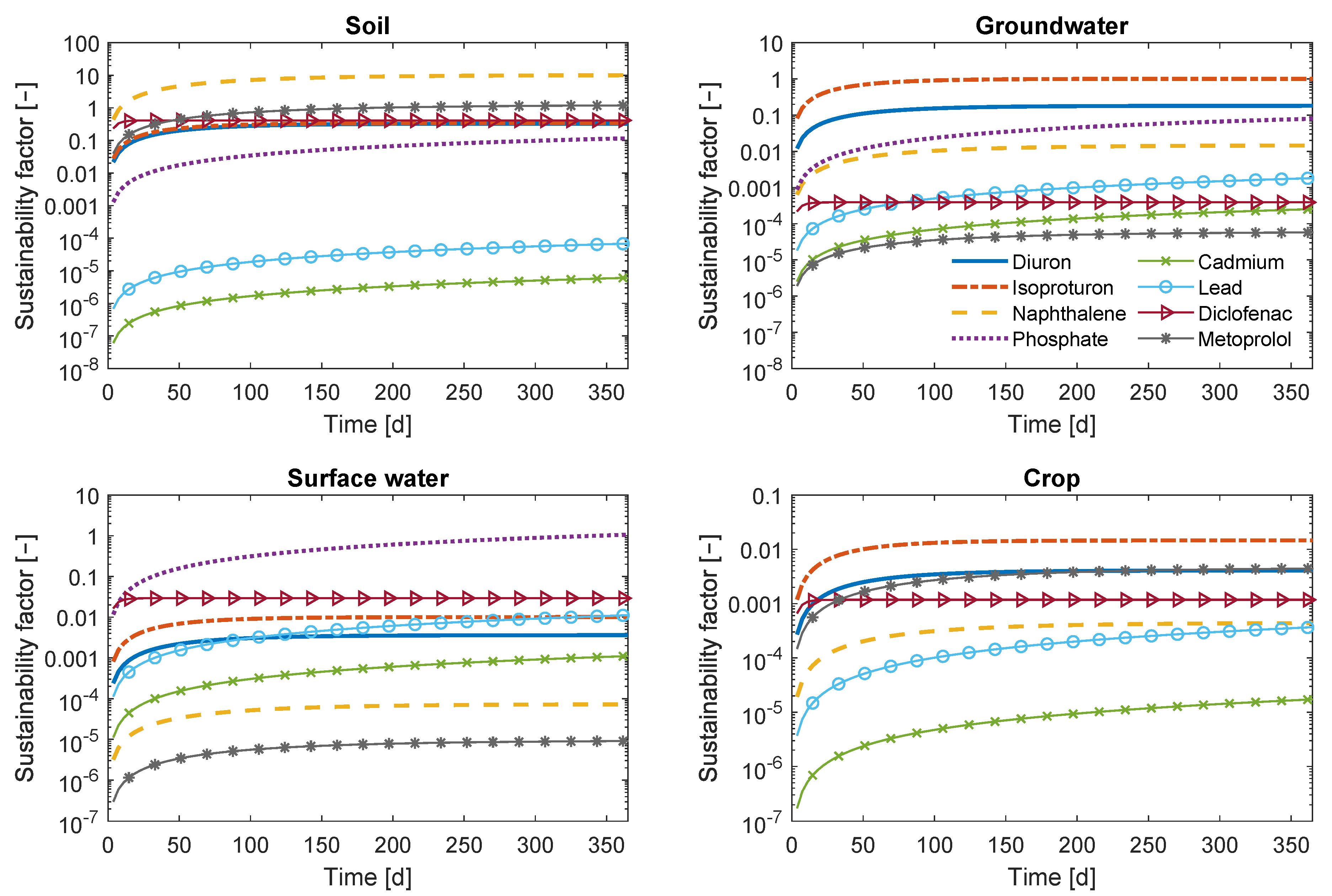
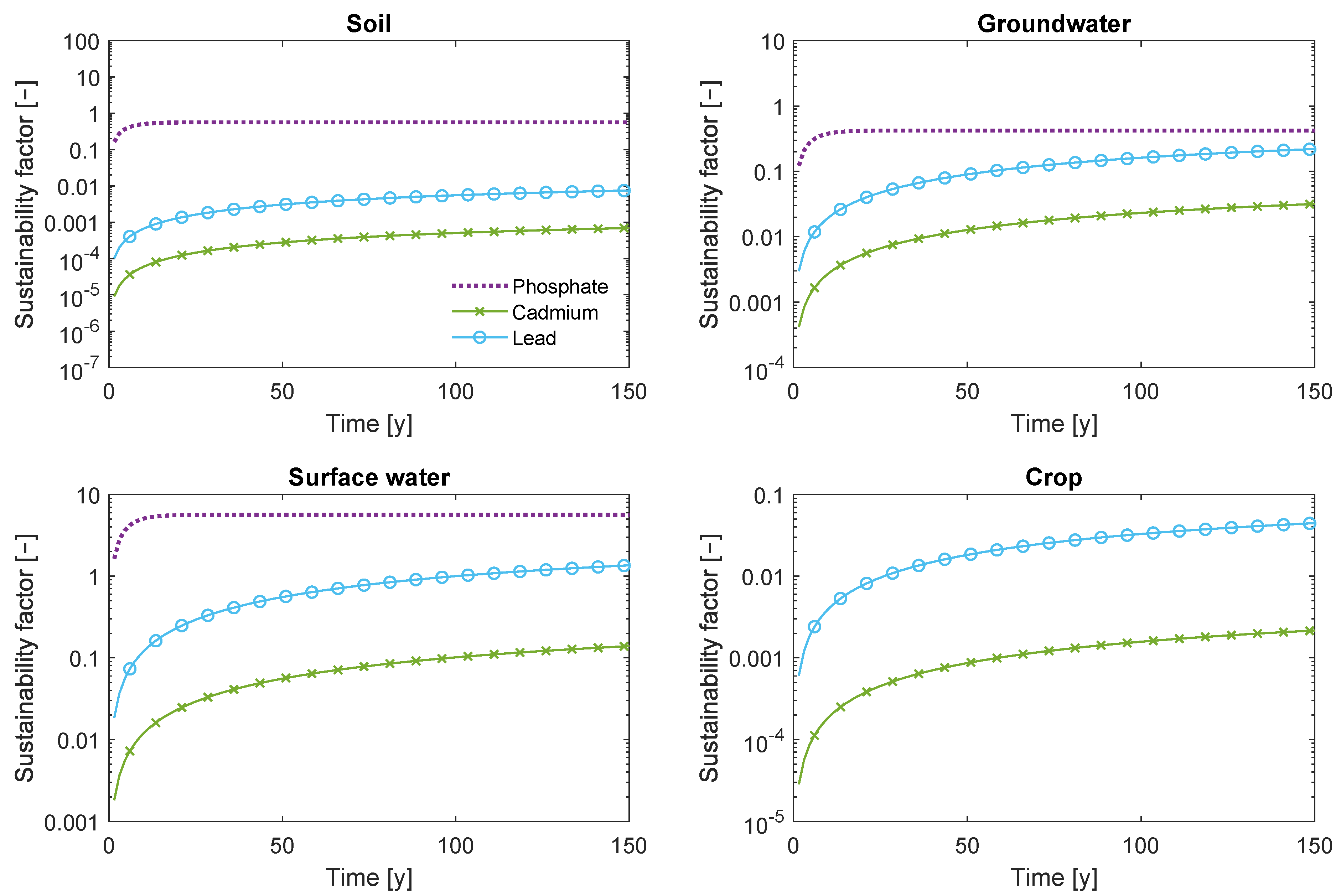
First, we consider the individual sustainability factors of each environmental compartment. There is a large difference in the time it takes to reach the concentration plateau (i.e., the steady state situation). Figure 2 shows the change in sustainability factors on the short term (i.e., one year). It can be observed that the plateau, is reached within a year for most contaminants. This means that if any violation of quality standards will occur for these contaminants, this will happen within a year. However, it takes over 20 years to reach the steady state situation for phosphate, since phosphate removal in the root zone is slow. The heavy metals cadmium and lead adsorb very strongly to the soil. For these contaminants, it takes centuries to reach the steady state situation, as can be seen from Figure 3, which shows the change of the sustainability factors over 150 years.

The soil quality standard is exceeded severely for naphthalene, and less severe for metoprolol. Both of these contaminants tend to accumulate in the soil, because of their relatively large adsorption coefficient (the largest of all the contaminants considered here) in combination with a relatively large half-life. The soil quality standard for naphthalene is exceeded within several days, while it takes over 150 days to that quality standard for metoprolol.

Only the groundwater quality standard of isoproturon is exceeded, which takes about 100 days. This contaminant has a relatively low adsorption coefficient, and is therefore very mobile and prone to leaching. Additionally, the groundwater quality standard for isoproturon is relatively small compared to the quality standards of the other contaminants considered here. Diclofenac has an even lower adsorption coefficient, but its half-life is much shorter, and thus most of it is removed by biodegradation instead of leaching.

From Figure 2, the exceedance of the surface water quality standard is not apparent for lead, and may not seem severe when looking at the short timescale of Figure 2, since the steady state situation is not yet reached within this timeframe. However, from Figure 3, we observe that the surface water quality standards are exceeded severely for lead and phosphate by a factor of 2.8 and 5.6, respectively.

Quality standards for crop and air are not exceeded by any of the contaminants. The air compartment is omitted from Figure 2, since the air quality standard is only defined for naphthalene. Naphthalene does not pose a risk to the air quality, as the sustainability factor for air equals $1.92\times {10}^{-5}$ at steady state.

The information of each sustainability factor is integrated into the sustainability indices, which are shown in

Table 3. The sustainability indices for each contaminant, showing the discrepancy factor $F_d$, the critical sustainability factor $F_c$, and the critical sustainability time $t_c$. The latter is only defined for contaminants whose quality standards are exceeded.

	${\mathit{F}}_{\mathit{d}}$ [-]	${\mathit{F}}_{\mathit{c}}$ [-]	${\mathit{t}}_{\mathit{c}}$ [d]
Diuron	$5.24\times {10}^{-3}$	0.33	n/a
Isoproturon	$1.99\times {10}^{-2}$	1.10	101
Naphthalene	$1.55\times {10}^{-4}$	10.17	8
Phosphate	3.63	5.63	312
Cadmium	$6.13\times {10}^{-2}$	0.31	n/a
Lead	0.68	2.79	36,556
Diclofenac	$5.12\times {10}^{-2}$	0.41	n/a
Metoprolol	$1.25\times {10}^{-4}$	1.24	185

for all the contaminants. The critical sustainability factors of isoproturon, naphthalene, phosphate, lead, and metoprolol are all larger than 1, ranging from 1.10 to 10.17. This indicates that quality standards are exceeded for these contaminants. In contrast, the critical sustainability factors of the other contaminants are smaller than 1, which indicates that no problems are expected to occur for these contaminants. The time it takes to exceed the quality standards depends on factors such as the input and output rates, the quality standard, and adsorption. Therefore, the critical sustainability time differs greatly between the different contaminants. For naphthalene, the soil quality standard is already exceeded within 9 days, while it takes several months to up to one year to exceed quality standards for isoproturon, metoprolol, and phosphate. However, for lead, which adsorbs strongly to the soil and does not degrade, the critical sustainability time exceeds 100 years. These differences are indicative of the differences in urgency regarding mitigation interventions.

Aside from phosphate, the discrepancy factor is smaller than 1 for all contaminants, which would indicate that no problems are expected to occur. However, the critical sustainability factors of both isoproturon and naphthalene exceed 1, which indicates that at least one quality standard of these contaminants is exceeded. As we mentioned earlier, the discrepancy factor identifies mostly if quality standards are exceeded severely; it is not a good indicator if such standards are violated slightly, such as for isoproturon in this example. Hence, a discrepancy factor larger than 1 indicates that problems will definitely occur, but a value lower than 1 does not mean the opposite. Additionally, the definition of the discrepancy factor does not consider accumulation in the soil. The potential risks of contaminants, such as the strongly adsorbing contaminants naphthalene and metoprolol in our example, are therefore not recognized. For these reasons, we do not recommend the use of the discrepancy factor as the only indicator of sustainability.

In this case study, the quality of the irrigation water is thus insufficient for long-term irrigation. Either further treatment of the wastewater used for irrigation or an alternative irrigation regime is required. The sustainability indices comprehensibly indicate which contaminants harm the public health and the environment based on the irrigation water quality and site-specific parameters. This allows for the identification of problematic contaminants, such that these specific contaminants can be prioritized during wastewater treatment.

3.2.2. Sensitivity Analysis

We show the sensitivity of the sustainability indices to the input parameters in

Table 4. The response of the critical sustainability factor $F_c$ and critical sustainability time $t_c$ in response to decreases and increases of 10% of the adsorption coefficient k, the degradation rate constant $\lambda$, the drainage rate q, and the evapotranspiration rate T. The critical sustainability time is only shown for contaminants whose standards are violated, as this parameter is otherwise undefined.

	k		$\mathit{\lambda }$		q		T		I
$F_c$	−10%	+10%	−10%	+10%	−10%	+10%	−10%	+10%	−10%	+10%
Diuron	0.33	0.33	0.37	0.30	0.33	0.33	0.33	0.33	0.30	0.36
Isoproturon	1.22	1.01	1.23	1.01	1.10	1.10	1.11	1.10	0.99	1.22
Naphthalene	10.17	10.18	11.30	9.25	10.17	10.17	10.18	10.17	9.16	11.19
Phosphate	5.64	5.63	5.64	5.64	5.70	5.57	6.17	5.18	5.07	6.20
Cadmium	0.35	0.29	0.31	0.31	0.32	0.31	0.32	0.31	0.28	0.35
Lead	3.03	2.59	2.80	2.80	2.83	2.76	2.82	2.77	2.52	3.08
Diclofenac	0.41	0.41	0.46	0.38	0.41	0.41	0.41	0.41	0.37	0.46
Metoprolol	1.24	1.24	1.38	1.13	1.24	1.24	1.24	1.24	1.12	1.36
$t_c$	−10%	+10%	−10%	+10%	−10%	+10%	−10%	+10%	−10%	+10%
Isoproturon	73	208	81	204	101	101	101	102	n/a	74
Naphthalene	8	8	8	9	8	8	8	8	9	8
Phosphate	281	342	312	312	311	312	309	315	350	281
Lead	32,255	41,046	36,556	36,556	36,431	36,682	36,479	36,633	41,830	32,478
Metoprolol	185	184	162	222	185	185	184	185	254	149

. The input parameters which are expected to have the most uncertainty are the adsorption coefficient and the degradation rate constant [79,80]. Additionally, there may also be significant uncertainty in the drainage, evapotranspiration, and irrigation rates [79,81].

The sensitivity of the sustainability indices to the input parameters differs for each contaminant, as it depends on factors such as the dominant transport process, the value of the critical sustainability factor, and which environmental compartment controls the critical sustainability factor.

For most cases, the dominant transport process is the main factor that drives the sensitivity of the sustainability indices to the input parameters. For all contaminants that degrade, degradation is the dominant removal process. Therefore, all degrading contaminants are greatly sensitive to errors in the degradation rate constant. None of the contaminants in this case study are sensitive to the drainage rate, since leaching is a minor removal process compared to the other removal processes. Only phosphate is sensitive to the evapotranspiration, as this is the only contaminant where plant uptake is an important removal process. Removal by soil erosion is the dominant transport process for cadmium and lead, while degradation in the adsorbed phase for isoproturon. The sustainability indices of these contaminants are therefore sensitive to the adsorption coefficient.

However, not everything can be explained by the dominant transport processes when we look at the adsorption coefficient. For example, degradation in the adsorbed phase is the dominant removal process for diuron, naphthalene, diclofenac, and metoprolol. Nevertheless, these contaminants are not sensitive to the adsorption coefficient. The critical sustainability factors of these contaminants are all determined by the soil quality standard. On the one hand, adsorption enhances contaminant accumulation in the soil, and on the other hand there is increased removal by degradation in the adsorbed phase and soil erosion. These two opposing effects nearly cancel each other out.

Within our framework, irrigation water is the only source of contaminant input. The contaminant concentration in the root zone at steady state is therefore a linear function of the irrigation rate, as can be derived from Equation (6). Naturally, the sustainability indices are therefore very sensitive to the irrigation rate. However, the annual irrigation rate may be estimated with more certainty than the other parameters considered in the sensitivity analysis. While not shown here, the sensitivity of the sustainability indices to the input concentration (i.e., the concentration of contaminants in the irrigation water) is equal to its sensitivity to the irrigation rate.

Additionally, the value of the critical sustainability factor also plays a role for the sensitivity of the critical sustainability time to input parameters. When the critical sustainability factor is close to one, the critical sustainability time becomes more sensitive.

Keeping these mechanisms in mind, it becomes possible to identify what the key parameters are for each contaminant. These key parameters can then be prioritized to be determined with great precision. Even when there are errors in the input parameters, the key parameters can still be identified, as long as the erroneous input parameters are still on the same order of magnitude as the correct values.

4. Discussion and Conclusions

In this study, we proposed a framework for the integrated sustainability assessment of irrigation with marginal water based on the work of Moolenaar et al. [46]. At this point, it is worthwhile to mention that the overall framework would also be applicable to other situations, such as the application of (bio)sludges or bulk waste materials at the soil surface. However, in those cases, the processes involving changes to those sludges and materials such as the mineralization of organic matter and subsequent changes in soil bulk density, soil hydraulic properties and related effects, need to be accounted for also. Since these are modifications of the root zone, this complicates the framework, but do not alter its essence.

Currently, quality standards for the various environmental compartments have been developed and are often applied separately. However, the contaminant fluxes to each compartment are coupled. Therefore, the benefit of the developed framework is that we comprehensively integrate the quality standards of different environmental compartments. This framework is made operational by two sustainability indices, that give information on which contaminants will violate quality standards, which environmental compartments are at risk, and on what timescale standards will be exceeded.

The results of the case study show that the time scales at which problems occur varies tremendously between different contaminants. The different time scales to reach the maximum values illustrate that reactivity plays a central role in how fast deterioration occurs, and that exceedance of quality standards differs for different environmental compartments. This is of direct importance for the urgency to take measures for better sustainability management.

The uncertainty in the input parameters, especially the adsorption coefficient and degradation rate constant, can potentially significantly affect the results of the sustainability assessment. However, the sensitivity of the sustainability indices to these parameters differs per contaminant species, and mostly depends on the dominant transport process for the contaminant. It is therefore valuable to determine the dominant transport process beforehand. This can be estimated from the transport parameters, for example with the use of Damköhler numbers [43].

The current framework is an extension to the work of Moolenaar et al. [46], which focused on and illustrated the benefit of integrating compartments for heavy metals. By adding transport processes such as biodegradation, erosion, and volatilization, the framework is applicable to a much broader range of contaminants. Another difference with the work of Moolenaar et al. [46] is that we de-valued the discrepancy factor. The discrepancy factor was originally meant to be a first indicator of potential problems, which could be estimated with relatively few assumptions and simple calculations. However, we have shown here that the discrepancy factor is an indicator that is appropriate for severe violations of environmental standards, but mild violations of quality standards may be masked.

The core of the framework consists of comparing contaminant fluxes to quality standards of the relevant environmental compartments. However, in many countries, quality standards for the environmental compartments have not been defined, or have been defined despite recognized flaws. Moreover, quality standards are lacking at all for many CECs, as awareness of these contaminants is recent and quantification of their pathways in the environment is still limited [82]. The framework cannot be applied in such cases, but these shortcomings do not invalidate its concept. Rather, a limited application to those compartments where constraints have been defined emphasizes where additional environmental quality standards are needed. In the example application, soil quality standards were not available for diclofenac and metoprolol. Therefore, we used the soil quality standard of permethrin instead, which is also a pharmaceutical. However, diclofenac is a non-steroidal anti-inflammatory drug, and metoprolol is a beta-blocker, while permethrin is an insecticide. Therefore, quality standards for diclofenac and metoprolol may be expected to be less toxic, and thus the quality standards in this example may be too strict. The same applies to the crop quality standard, for which no information was available for naphthalene, diclofenac, and metoprolol. Instead, we used the same quality standards as for the pesticides diuron and isoproturon, which might be more strict than necessary for the pharmaceuticals considered here. Naturally, with disputable quality standards as in our example, the framework will give a disputable outcome, but may help to identify gaps and weaknesses and give a rational basis for improvement.

Though our work aims to indicate how different standards of different environmental compartments as soil, crop, and groundwater may be used to assess sustainability of soil and water management in an integrated fashion, we already mentioned that this requires that such standards are available. The development of such standards and their foundation (whether (eco)toxicological or otherwise) is, of course, an active field of research [83]. For instance, synergistic and antagonistic effects of contaminant mixtures on biota may affect the associated hazards [84]. Particularly for treated waste water, this may reflect on how quality standards for compartments such as soil or water should be adjusted to appropriately account for those hazards. Though relevant for this investigation, the development of environmental standards as such is not the aim of this paper. Rather, if appropriate standards have been agreed upon, we show how to harmonize them for different compartments. As we showed, also uncertainty of other model parameters affects the outcome. The involved uncertainty in our framework’s results, as in other environmental assessments, remains a persistent and hard to tackle issue in environmental management. As current environmental standards reveal, management cannot wait until such issues are satisfactorily resolved.

Recognizing that absent or flawed environmental standards and uncertainty or bias in parameters affect the value of our integrated sustainability framework, as indeed environmental assessments in general, the framework has several benefits. It gives an integrated perspective to appreciate environmental contamination of different compartments and inspires where mitigating interventions might be most effective and have the highest priority. Where appropriate standards are missing or flawed, it may help to recognize how important that is, compared with the impacts on other compartments which can be quantified to satisfaction. Even so, the integrated framework is no panacea, but a useful ingredient to assessment of our management choices.

References

- Sarhadi, A.; Burn, D.H.; Johnson, F.; Mehrotra, R.; Sharma, A. Water resources climate change projections using supervised nonlinear and multivariate soft computing techniques. J. Hydrol. 2016, 536, 119–132. [Google Scholar] [CrossRef] [Green Version]
- Ali, A.M.; Shafiee, M.E.; Berglund, E.Z. Agent-based modeling to simulate the dynamics of urban water supply: Climate, population growth, and water shortages. Sustain. Cities Soc. 2017, 28, 420–434. [Google Scholar]
- United Nations Development Programme (UNDP). Beyond Scarcity: Power, Poverty and the Global Water Crisis; Human Development Report; Palgrave Macmillan: New York, NY, USA, 2006; Available online: https://www.undp.org/content/undp/en/home/librarypage/hdr/human-development-report-2006.html (accessed on 22 April 2021).
- UNESCO-WWAP. 1st UN World Water Development Report: Water for People, Water for Life; UNESCO and Berghahn Books: New York, NY, USA, 2003. [Google Scholar]
- Hamilton, A.J.; Stagnitti, F.; Xiong, X.; Kreidl, S.L.; Benke, K.K.; Maher, P. Wastewater Irrigation: The State of Play. Vadose Zone J. 2007, 6, 823–840. [Google Scholar] [CrossRef] [Green Version]
- Bixio, D.; Thoeye, C.; De Koning, J.; Joksimovic, D.; Savic, D.; Wintgens, T.; Melin, T. Wastewater reuse in Europe. Desalination 2006, 187, 89–101. [Google Scholar] [CrossRef]
- Toze, S. Reuse of effluent water—benefits and risks. Agric. Water Manag. 2006, 80, 147–159. [Google Scholar] [CrossRef] [Green Version]
- Al-Nakshabandi, G.; Saqqar, M.; Shatanawi, M.; Fayyad, M.; Al-Horani, H. Some environmental problems associated with the use of treated wastewater for irrigation in Jordan. Agric. Water Manag. 1997, 34, 81–94. [Google Scholar] [CrossRef]
- Metcalf, L.; Harrison, P.E.; Tchobanoglous, G. Wastewater Engineering: Treatment, Disposal, and Reuse; McGraw-Hill: New York, NY, USA, 2004; Volume 4. [Google Scholar]
- Petrović, M.; Gonzalez, S.; Barceló, D. Analysis and removal of emerging contaminants in wastewater and drinking water. Trends Anal. Chem. 2003, 22, 685–696. [Google Scholar] [CrossRef] [Green Version]
- Kim, S.; Chu, K.H.; Al-Hamadani, Y.A.; Park, C.M.; Jang, M.; Kim, D.H.; Yu, M.; Heo, J.; Yoon, Y. Removal of contaminants of emerging concern by membranes in water and wastewater: A review. Chem. Eng. J. 2018, 335, 896–914. [Google Scholar] [CrossRef]
- Mapanda, F.; Mangwayana, E.; Nyamangara, J.; Giller, K. The effect of long-term irrigation using wastewater on heavy metal contents of soils under vegetables in Harare, Zimbabwe. Agric. Ecosyst. Environ. 2005, 107, 151–165. [Google Scholar] [CrossRef]
- Rezapour, S.; Samadi, A.; Khodaverdiloo, H. An Investigation of the Soil Property Changes and Heavy Metal Accumulation in Relation to Long-term Wastewater Irrigation in the Semi-arid Region of Iran. Soil Sediment Contam. 2011, 20, 841–856. [Google Scholar] [CrossRef]
- Farahat, E.; Linderholm, H.W. The effect of long-term wastewater irrigation on accumulation and transfer of heavy metals in Cupressus sempervirens leaves and adjacent soils. Sci. Total Environ. 2015, 512–513, 1–7. [Google Scholar] [CrossRef] [PubMed]
- Jalali, M.; Merikhpour, H.; Kaledhonkar, M.; Van Der Zee, S.E.A.T.M. Effects of wastewater irrigation on soil sodicity and nutrient leaching in calcareous soils. Agric. Water Manag. 2008, 95, 143–153. [Google Scholar] [CrossRef]
- Muyen, Z.; Moore, G.A.; Wrigley, R.J. Soil salinity and sodicity effects of wastewater irrigation in South East Australia. Agric. Water Manag. 2011, 99, 33–41. [Google Scholar] [CrossRef]
- Tunc, T.; Sahin, U. The changes in the physical and hydraulic properties of a loamy soil under irrigation with simpler-reclaimed wastewaters. Agric. Water Manag. 2015, 158, 213–224. [Google Scholar] [CrossRef]
- Tang, C.; Chen, J.; Shindo, S.; Sakura, Y.; Zhang, W.; Shen, Y. Assessment of groundwater contamination by nitrates associated with wastewater irrigation: A case study in Shijiazhuang region, China. Hydrol. Process. 2004, 18, 2303–2312. [Google Scholar] [CrossRef]
- Pereira, B.F.F.; He, Z.; Stoffella, P.J.; Montes, C.R.; Melfi, A.J.; Baligar, V.C. Nutrients and Nonessential Elements in Soil after 11 Years of Wastewater Irrigation. J. Environ. Qual. 2012, 41, 920–927. [Google Scholar] [CrossRef] [Green Version]
- Paruch, A.M. The impact of wastewater irrigation on the chemical quality of groundwater. Water Environ. J. 2014, 28, 502–508. [Google Scholar] [CrossRef]
- Chen, C.; Li, J.; Chen, P.; Ding, R.; Zhang, P.; Li, X. Occurrence of antibiotics and antibiotic resistances in soils from wastewater irrigation areas in Beijing and Tianjin, China. Environ. Pollut. 2014, 193, 94–101. [Google Scholar] [CrossRef]
- Woodward, E.E.; Andrews, D.M.; Williams, C.F.; Watson, J.E. Vadose Zone Transport of Natural and Synthetic Estrogen Hormones at Penn State’s “Living Filter” Wastewater Irrigation Site. J. Environ. Qual. 2014, 43, 1933–1941. [Google Scholar] [CrossRef]
- Wang, S.; Wu, W.; Liu, F.; Yin, S.; Bao, Z.; Liu, H. Spatial distribution and migration of nonylphenol in groundwater following long-term wastewater irrigation. J. Contam. Hydrol. 2015, 177–178, 85–92. [Google Scholar] [CrossRef]
- World Health Organization (WHO). Guidelines for the Safe Use of Wastewater, Excreta and Greywater; Technical Report; World Health Organization: Geneva, Switzerland, 2006; Volume 4, Available online: https://www.who.int/water_sanitation_health/publications/gsuweg4/en/ (accessed on 22 April 2021).
- United States Environmental Protection Agency (US EPA). Guidelines for Water Reuse; Technical Report EPA/600/R-12/618; United States Environmental Protection Agency: Washington, DC, USA, 2012.
- European Council. Regulation of the European Parliament and of the Council on Minimum Requirements for Water Reuse. 2019. Available online: https://www.consilium.europa.eu/en/press/press-releases/2020/04/07/water-reuse-for-agricultural-irrigation-council-adopts-new-rules/ (accessed on 22 April 2021).
- Rizzo, L.; Krätke, R.; Linders, J.; Scott, M.; Vighi, M.; de Voogt, P. Proposed EU minimum quality requirements for water reuse in agricultural irrigation and aquifer recharge: SCHEER scientific advice. Curr. Opin. Environ. Sci. Health 2018, 2, 7–11. [Google Scholar] [CrossRef]
- Weber, S.; Khan, S.; Hollender, J. Human risk assessment of organic contaminants in reclaimed wastewater used for irrigation. Desalination 2006, 187, 53–64. [Google Scholar] [CrossRef] [Green Version]
- Troldborg, M.; Duckett, D.; Allan, R.; Hastings, E.; Hough, R.L. A risk-based approach for developing standards for irrigation with reclaimed water. Water Res. 2017, 126, 372–384. [Google Scholar] [CrossRef]
- Qian, Y.L.; Mecham, B. Long-Term Effects of Recycled Wastewater Irrigation on Soil Chemical Properties on Golf Course Fairways. Agron. J. 2005, 97, 717–721. [Google Scholar] [CrossRef]
- Virto, I.; Bescansa, P.; Imaz, M.; Enrique, A. Soil quality under food-processing wastewater irrigation in semi-arid land, northern Spain: Aggregation and organic matter fractions. J. Soil Water Conserv. 2006, 61, 398–407. [Google Scholar]
- Xu, J.; Wu, L.; Chang, A.C.; Zhang, Y. Impact of long-term reclaimed wastewater irrigation on agricultural soils: A preliminary assessment. J. Hazard. Mater. 2010, 183, 780–786. [Google Scholar] [CrossRef]
- Rezapour, S.; Samadi, A. Soil quality response to long-term wastewater irrigation in Inceptisols from a semi-arid environment. Nutr. Cycl. Agroecosyst. 2011, 91, 269–280. [Google Scholar] [CrossRef]
- Razzaghi, S.; Khodaverdiloo, H.; Dashtaki, S.G. Effects of long-term wastewater irrigation on soil physical properties and performance of selected infiltration models in a semi-arid region. Hydrol. Sci. J. 2016, 61, 1778–1790. [Google Scholar] [CrossRef]
- Chiou, C.T.; Sheng, G.; Manes, M. A Partition-Limited Model for the Plant Uptake of Organic Contaminants from Soil and Water. Environ. Sci. Technol. 2001, 35, 1437–1444. [Google Scholar] [CrossRef]
- Jjemba, P.K. The effect of chloroquine, quinacrine, and metronidazole on both soybean plants and soil microbiota. Chemosphere 2002, 46, 1019–1025. [Google Scholar] [CrossRef]
- Pedrero, F.; Alarcón, J.J. Effects of treated wastewater irrigation on lemon trees. Desalination 2009, 246, 631–639. [Google Scholar] [CrossRef]
- Gallegos, E.; Warren, A.; Robles, E.; Campoy, E.; Calderon, A.; Sainz, M.G.; Bonilla, P.; Escolero, O. The effects of wastewater irrigation on groundwater quality in Mexico. Water Sci. Technol. 1999, 40, 45–52. [Google Scholar] [CrossRef]
- Candela, L.; Fabregat, S.; Josa, A.; Suriol, J.; Vigués, N.; Mas, J. Assessment of soil and groundwater impacts by treated urban wastewater reuse. A case study: Application in a golf course (Girona, Spain). Sci. Total Environ. 2007, 374, 26–35. [Google Scholar] [CrossRef] [PubMed]
- Pedersen, J.A.; Soliman, M.; Suffet, I.H.M. Human Pharmaceuticals, Hormones, and Personal Care Product Ingredients in Runoff from Agricultural Fields Irrigated with Treated Wastewater. J. Agric. Food Chem. 2005, 53, 1625–1632. [Google Scholar] [CrossRef] [PubMed]
- Jury, W.A.; Russo, D.; Streile, G.; El Abd, H. Evaluation of volatilization by organic chemicals residing below the soil surface. Water Resour. Res. 1990, 26, 13–20. [Google Scholar] [CrossRef]
- Wildenschild, D.; Jensen, K.H. Numerical modeling of observed effective flow behavior in unsaturated heterogeneous sands. Water Resour. Res. 1999, 35, 29–42. [Google Scholar] [CrossRef]
- Cornelissen, P.; Van der Zee, S.E.A.T.M.; Leijnse, A. Role of degradation concepts for adsorbing contaminants in context of wastewater irrigation. Vadose Zone J. 2020, 19, e20064. [Google Scholar] [CrossRef]
- Boivin, A.; Cherrier, R.; Schiavon, M. A comparison of five pesticides adsorption and desorption processes in thirteen contrasting field soils. Chemosphere 2005, 61, 668–676. [Google Scholar] [CrossRef] [PubMed]
- Kodešová, R.; Grabic, R.; Kočárek, M.; Klement, A.; Golovko, O.; Fér, M.; Nikodem, A.; Jakšík, O. Pharmaceuticals’ sorptions relative to properties of thirteen different soils. Sci. Total Environ. 2015, 511, 435–443. [Google Scholar] [CrossRef] [PubMed]
- Moolenaar, S.W.; Van Der Zee, S.E.A.T.M.; Lexmond, T.M. Indicators of the sustainability of heavy-metal management in agro-ecosystems. Sci. Total Environ. 1997, 201, 155–169. [Google Scholar] [CrossRef]
- European Council. Regulation (EC) No 1907/2006 of the European Parliament and of the Council. 2006. Available online: https://eur-lex.europa.eu/legal-content/EN/TXT/?uri=CELEX%3A02006R1907-20140410 (accessed on 22 April 2021).
- Van De Craats, D.; Van Der Zee, S.E.A.T.M.; Sui, C.; Van Asten, P.J.A.; Cornelissen, P.; Leijnse, A. Soil sodicity originating from marginal groundwater. Vadose Zone J. 2020, 19, e20010. [Google Scholar] [CrossRef]
- Boekhold, A.E.; Van Der Zee, S.E.A.T.M. Long-term effects of soil heterogeneity on cadmium behaviour in soil. J. Contam. Hydrol. 1991, 7, 371–390. [Google Scholar] [CrossRef]
- Jaramillo, M.F.; Restrepo, I. Wastewater reuse in agriculture: A review about its limitations and benefits. Sustainability 2017, 9, 1734. [Google Scholar] [CrossRef] [Green Version]
- Allen, R.G.; Pereira, L.S.; Raes, D.; Smith, M. Crop evapotranspiration—Guidelines for computing crop water requirements. FAO Irr. Drain. Pap. 1998, 56, 110. [Google Scholar]
- Minasny, B.; McBratney, A.B. The efficiency of various approaches to obtaining estimates of soil hydraulic properties. Geoderma 2002, 107, 55–70. [Google Scholar] [CrossRef]
- United States Department of Agriculture, Natural Resources Conservation Service (USDA NRCS). 2014; Soil Bulk Density/Moisture/Aeration. Available online: https://www.nrcs.usda.gov/Internet/FSE_DOCUMENTS/nrcs142p2_053260.pdf (accessed on 22 April 2021).
- Van Der Meer, R.W. Watergebruik in de Land- en Tuinbouw 2017 en 2018; Technical Report Nota 2020-030, Wageningen Economic Research; Wageningen: Gelderland, The Netherlands, 2020. [Google Scholar]
- Royal Dutch Meteorological Institute (KNMI). Overzicht van de Neerslag en Verdamping in Nederland. 2020. Available online: https://www.knmi.nl/nederland-nu/klimatologie/gegevens/monv (accessed on 22 April 2021).
- Kwaad, F.J.P.M. Summer and winter regimes of runoff generation and soil erosion on cultivated loess soils (The Netherlands). Earth Surf. Process. Landf. 1991, 16, 653–662. [Google Scholar] [CrossRef]
- Muñoz, I.; Gómez-Ramos, M.J.; Agüera, A.; Fernández-Alba, A.R.; García-Reyes, J.F.; Molina-Díaz, A. Chemical evaluation of contaminants in wastewater effluents and the environmental risk of reusing effluents in agriculture. Trends Anal. Chem. 2009, 28, 676–694. [Google Scholar] [CrossRef]
- European Commission. Technical Guidance Document on Risk Assessment, Part II; Report EUR 20418 EN/2; European Chemicals Bureau, Institute for Health and Consumer Protection: Ispra, Italy, 2003. [Google Scholar]
- Briggs, G.G.; Bromilow, R.H.; Evans, A.A. Relationships between lipophilicity and root uptake and translocation of non-ionised chemicals by barley. Pestic. Sci. 1982, 13, 495–504. [Google Scholar] [CrossRef]
- Kim, S.; Chen, J.; Cheng, T.; Gindulyte, A.; He, J.; He, S.; Li, Q. and Shoemaker, B.A.; Thiessen, P.A.; Yu, B.; Zaslavsky, L.; Zhang, J.; Bolton, E.E. PubChem 2019 update: Improved access to chemical data. Nucleic Acids Res. 2019, 47, D1102–D1109. [Google Scholar] [CrossRef] [PubMed] [Green Version]
- National Institute for Public Health and the Environment (RIVM). Zoeksysteem Risico’s van Stoffen. Available online: https://rvszoeksysteem.rivm.nl/stoffen (accessed on 22 April 2021).
- European Commission. Proposal for a Directive of the European Parliament and of the Council amending Directives 2000/60/EC and 2008/105/EC as Regards Priority Substances in the Field of Water Policy. 2011. Available online: https://op.europa.eu/en/publication-detail/-/publication/859825c3-d7c7-424b-96dd-84eb700ef0bf (accessed on 22 April 2021).
- Verenigde Telers Akkerbouw (VTA). Opbrengst uien. 2019. Available online: https://www.vtanederland.nl/opbrengst-uien-ongeveer-op-langjarig-gemiddelde (accessed on 22 April 2021).
- European Council. On Maximum Residue Levels of Pesticides in or on Food and Feed of Plant and Animal Origin and Amending Council Directive 91/414/EEC. 2005. Available online: https://eur-lex.europa.eu/legal-content/EN/ALL/?uri=CELEX%3A32005R0396 (accessed on 22 April 2021).
- Bouwer, H.; Idelovitch, E. Quality requirements for irrigation with sewage water. J. Irrig. Drain. Eng. 1987, 113, 516–535. [Google Scholar] [CrossRef]
- Liu, Y.; Xu, Z.; Wu, X.; Gui, W.; Zhu, G. Adsorption and desorption behavior of herbicide diuron on various Chinese cultivated soils. J. Hazard. Mater. 2010, 178, 462–468. [Google Scholar] [CrossRef] [PubMed]
- Carmo, A.M.; Hundal, L.S.; Thompson, M.L. Sorption of Hydrophobic Organic Compounds by Soil Materials: Application of Unit Equivalent Freundlich Coefficients. Environ. Sci. Technol. 2000, 34, 4363–4369. [Google Scholar] [CrossRef]
- Debicka, M.; Kocowicz, A.; Weber, J.; Jamroz, E. Organic matter effects on phosphorus sorption in sandy soils. Arch. Agron. Soil Sci. 2016, 62, 840–855. [Google Scholar] [CrossRef]
- Rouchaud, J.; Neus, O.; Bulcke, R.; Cools, K.; Eelen, H.; Dekkers, T. Soil Dissipation of Diuron, Chlorotoluron, Simazine, Propyzamide, and Diflufenican Herbicides After Repeated Applications in Fruit Tree Orchards. Arch. Environ. Contam. Toxicol. 2000, 39, 60–65. [Google Scholar] [CrossRef]
- Walker, A.; Jurado-Exposito, M.; Bending, G.; Smith, V. Spatial variability in the degradation rate of isoproturon in soil. Environ. Pollut. 2001, 111, 407–415. [Google Scholar] [CrossRef]
- Thiele-Bruhn, S.; Brümmer, G.W. Kinetics of Polycyclic Aromatic Hydrocarbon (PAH) Degradation in Long-term Polluted Soils during Bioremediation. Plant Soil 2005, 275, 31–42. [Google Scholar] [CrossRef]
- Sander, R. Compilation of Henry’s law constants (version 4.0) for water as solvent. Atmos. Chem. Phys. 2015, 15, 4399–4981. [Google Scholar] [CrossRef] [Green Version]
- Dutch Ministry of Health, Welfare and Sport. Warenwetregeling Verontreinigingen in levensmiddelen. Staatscourant 1999, 30, 11. Available online: https://zoek.officielebekendmakingen.nl/stcrt-1998-61-p8-SC13207.pdf (accessed on 22 April 2021).
- Lee, S.Z.; Allen, H.E.; Huang, C.P.; Sparks, D.L.; Sanders, P.F.; Peijnenburg, W.J.G.M. Predicting soil-water partition coefficients for cadmium. Environ. Sci. Technol. 1996, 30, 3418–3424. [Google Scholar] [CrossRef]
- Lee, S.Z.; Chang, L.; Yang, H.H.; Chen, C.M.; Liu, M.C. Adsorption characteristics of lead onto soils. J. Hazard. Mater. 1998, 63, 37–49. [Google Scholar] [CrossRef]
- Xu, J.; Wu, L.; Chang, A.C. Degradation and adsorption of selected pharmaceuticals and personal care products (PPCPs) in agricultural soils. Chemosphere 2009, 77, 1299–1305. [Google Scholar] [CrossRef] [PubMed]
- Kodešová, R.; Kočárek, M.; Klement, A.; Golovko, O.; Koba, O.; Fér, M.; Nikodem, A.; Vondráčková, L.; Jakšík, O.; Grabic, R. An analysis of the dissipation of pharmaceuticals under thirteen different soil conditions. Sci. Total Environ. 2016, 544, 369–381. [Google Scholar] [CrossRef] [PubMed]
- United States Environmental Protection Agency. Technical Appendix B, Physico-chemical Properties for TRI Chemicals and Chemical Categories. 2014. Available online: https://www.epa.gov/sites/production/files/2014-03/documents/tech_app_b_v215.pdf (accessed on 22 April 2021).
- Dubus, I.G.; Brown, C.D.; Beulke, S. Sensitivity analyses for four pesticide leaching models. Pest. Manag. Sci. 2003, 59, 962–982. [Google Scholar] [CrossRef] [PubMed]
- Lammoglia, S.K.; Brun, F.; Quemar, T.; Moeys, J.; Barriuso, E.; Gabrielle, B.; Mamy, L. Modelling pesticides leaching in cropping systems: Effect of uncertainties in climate, agricultural practices, soil and pesticide properties. Environ. Model. Softw. 2018, 109, 342–352. [Google Scholar] [CrossRef]
- Long, D.; Longuevergne, L.; Scanlon, B.R. Uncertainty in evapotranspiration from land surface modeling, remote sensing, and GRACE satellites. Water Resour. Res. 2014, 50, 1131–1151. [Google Scholar] [CrossRef] [Green Version]
- Lapworth, D.; Baran, N.; Stuart, M.; Ward, R. Emerging organic contaminants in groundwater: A review of sources, fate and occurrence. Environ. Pollut. 2012, 163, 287–303. [Google Scholar] [CrossRef] [Green Version]
- Lapworth, D.J.; Lopez, B.; Laabs, V.; Kozel, R.; Wolter, R.; Ward, R.; Amelin, E.V.; Besien, T.; Claessens, J.; Delloy, F. Developing a groundwater watch list for substances of emerging concern. Environ. Res. Lett. 2019, 14, 035004. [Google Scholar] [CrossRef] [Green Version]
- Barber, L.B.; Keefe, S.H.; Brown, G.K.; Furlong, E.T.; Gray, J.L.; Kolpin, D.W.; Meyer, M.T.; Sandstrom, M.W.; Zaugg, S.D. Persistence and potential effects of complex organic contaminant mixtures in wastewater-impacted streams. Environ. Sci. Technol. 2013, 47, 2177–2188. [Google Scholar] [CrossRef]
Figure 1.
A schematic representation of various environmental compartments relevant to irrigation with marginal water, indicating the possible contaminant pathways between compartments. Accumulation of contaminants in each end compartment can cause risks for public health and the environment.
Figure 2.
The short-term change of the sustainability factors over time, plotted for each contaminant and environmental compartment. Note the logarithmic scale of the y-axis.
Figure 3.
The long-term change of the sustainability factors over time in each environmental compartment, plotted for the persistent contaminants phosphate, cadmium, and lead. Note the logarithmic scale of the y-axis.