
Spatiotemporal Effects and Driving Factors of Water Pollutants Discharge in Beijing–Tianjin–Hebei Region


1
School of Urban and Environmental Science, Huaiyin Normal University, Huai’an 223300, China
2
College of Resources Environment and Tourism, Capital Normal University, Beijing 100048, China
*
Author to whom correspondence should be addressed.
Water 2021, 13(9), 1174; https://doi.org/10.3390/w13091174
Submission received: 24 March 2021
/
Revised: 19 April 2021
/
Accepted: 22 April 2021
/
Published: 24 April 2021
(This article belongs to the Special Issue Management and Monitoring of Urban and Rural Ecological Water Resources)
Abstract
:The problem of water pollution is a social issue in China requiring immediate and urgent solutions. In the Beijing–Tianjin–Hebei region, the contradiction between preserving the ecological environment and facilitating sustainable economic development is particularly acute. This study analyzed the spatiotemporal evolution of water pollutants and their factors of influence using statistics on the discharge of two water pollutants, namely chemical oxygen demand (COD) and NH3-N (ammonia nitrogen), in 154 counties in both 2012 and 2016 as research units in the region. The study employed Exploratory Spatial-Time Data Analysis (ESTDA), Standard Deviational Ellipse (SDE), and the Geographically Weighted Regression (GWR) models, as well as ArcGIS and GeoDa software, obtaining the following conclusions: (1) From 2012 to 2016, pollutant discharge dropped significantly, with COD and NH3-N emissions decreasing 65.9% and 47.2%, respectively; the pollutant emissions possessed the spatial feature of gradual gradient descent from the central districts to the periphery. (2) The water pollutants discharge displayed significant and positive spatial correlations. The spatiotemporal cohesion of the spatiotemporal evolution of the pollutants was higher than their spatiotemporal fluidity, representing strong spatial locking. (3) The level of economic development, the level of urbanization, and the intensity of agricultural production input significantly and positively drove pollutant discharge; the environmental regulations had a significant effect on reducing the emission of pollutants. In particular, the effect for NH3-N emissions reduction was stronger; the driving effect of the industrial structure and the distance decay was not significant.
1. Introduction
Since 1978, China’s Gross Regional Product (GDP) has grown at an average rate of 9.5% per year, considerably higher than the 2.9% growth rate of the world economy for the same period. Environmental pollution was the price for rapid economic growth, and the total discharge of pollutants in water environments remains high. For example, in 2016, the wastewater discharge in the country amounted to 71.11 billion tons; the emission of chemical oxygen demand (COD) in wastewater amounted to 10.465 million tons, and that of ammonia nitrogen (NH3-N) amounted to 1.418 million tons (data from China Statistical Yearbook,2017). Economic losses due to water pollution amounted to as much as RMB 240 billion [1]. Especially in urbanized areas with larger populations and economic agglomerations, the pressure exerted on the environmental system is substantial. According to the Report on the State of the Ecology and Environment in China, the proportion of water “inferior than Grade V” in the Haihe River Basin was 41.0% of the entire basin. Water pollution has severely restricted the improvement of human living environments and threatened the physical and mental health of residents [2,3]. Due to water pollution, severe water scarcity was observed in approximately 400 cities in China [4]. Thus, water pollution is a social issue urgently requiring immediate solutions [5].
COD is a key indicator of the degree of organic pollution in a waterbody. It has been widely applied in evaluating water pollution levels [6,7]. NH3 and NH4 (NH3-N) mainly originate from nitrogenous organic matter in domestic sewage and are decomposed into nitrite nitrogen in the waterbody through the action of microorganisms. Long-term consumption of water containing high nitrite nitrogen levels is harmful to human health. A crucial aspect of water pollution prevention is control of total pollutant discharge. In the eleventh Five-Year Plan in China, COD was officially included as a binding indicator for the control of the total pollutants countrywide. In the twelfth Five-Year Plan, NH3-N was included as a binding indicator for the control of the total pollutants countrywide; this had a considerable effect in alleviating water pollution. Meanwhile, academics approached water pollution by using measures including the spatial patterns of water pollutions [8], pollutant emission measurement [9], factors of influence for water pollutants [10], sources of pollutants [11], pollution emission reduction [12], and pollution control model optimization [13]; and they investigated water pollution and its prevention. Research has revealed that water pollution was the main cause of the lack of water resources in southern China [14]; the pollutant discharge in China’s water environment has had a substantial spatial agglomeration effect, and the sources of pollution were mainly manifested as three types, namely agricultural source-based, urban life source-based, and mixed urban life and agricultural source-based. The pollutant emission intensity in regions with agricultural source-based pollution was the highest [15]. COD emission was less sensitive to changes in industrial production; the expansion of manufacturing was the main reason for the increase of the quantity of COD in industrial wastewater, and technological progress has helped reduce its emission [16]. Research on regions has revealed that, in the Fujian Bay region, Meizhou Bay had the largest COD emissions, and agricultural pollution was predominant over industrial pollution [17].
The water pollutants discharge in Jiangsu Province exhibited a significant spatial correlation, and such a correlation in southern Jiangsu is higher than that in northern Jiangsu [18]. The spatial agglomeration characteristic of the environmental pollution in Jilin Province was significant; the spatial change represented more stable path locking [8] and the spatial correlations of water pollutants distribution in Wuxi City with textile, petrochemical, and metallurgical industries was higher [19]. There was a significant and positive coupling effect between pollution levels in water environment and degree of industrial enterprise agglomeration in Zhangjiakou City [20]. Regarding water pollution, studies have been conducted in river and lake basins, including the Taihu Lake Basin [21], Yangtze River Basin [22], Yellow River Basin [23], Zhuhe River Basin [24], Liaohe River Basin [25], Haihe River Basin [26], and Songhua River Basin [27] in China as well as in the Biñan River Basin in the Philippines [28]. The results have indicated that although water pollution prevention efforts had been made, the phenomenon of water pollution remained; in particular, the Haihe River Basin remain in the category of “heavy pollution,” and local water quality improvement has progressed slowly. Similar to pollutant discharge in China, water pollution in river basins has also had a large spatial agglomeration effect, and pollution emission reduction has also had a spatial effect. Increases in local pollution emissions were adverse to emission reduction in neighboring basins; the phenomenon of cross-border water pollution was severe, and strengthening the collaborative governance mechanism for regional pollution was a key to water pollution prevention.
In China, areas of urban agglomeration represent the main form of urbanization and are the crucial spatial vehicle for regional economic growth [29]. In 19 areas of urban agglomeration in China, 75.3% of China’s population and 88.1% of the country’s GDP are concentrated in 25% of the country’s land area. The highly concentrated population, economy, and industry have created acute problems for the ecological environment. The Beijing–Tianjin–Hebei area of urban agglomeration is the region with the most acute contradiction between protection of the ecological environment and sustainable economic development in China [30], and the basin with the highest level of water resources development and the most severe water pollution is the Haihe River Basin. Regional population size, industrial agglomeration, and economic development all have strong and positive effects on driving the discharge of water pollutants [31]. Beijing–Tianjin–Hebei, with 2.25% of the country’s land area, produces 5.75% of COD emissions and 5.83% of NH3-N emissions in the country; water pollution prevention there requires immediate attention. However, most research on water pollution in China has been on the national scale or the basin scale. Although studies have been conducted on the Bohai Rim region, they were generally conducted at the city scale, and research at the microscopic scale of the county remains to be pursued. In addition, most existing research on the driving factors of the discharge of water pollutants have adopted general linear models and ignored the spatial heterogeneity of factors. Thus, this study took the Beijing–Tianjin–Hebei regional counties as the space units (the basic research objects) and comprehensively used exploratory spatial-time data analysis (ESTDA), the Least Square Method (OLS), and the geographically weighted regression (GWR) model to analyze the spatiotemporal evolution of and driving factors for water pollutants discharge in the Beijing–Tianjin–Hebei counties of urban agglomerations. The study aimed to thoroughly explore and examine the status quo and the features of water pollution in these counties, and to provide a reference for prevention and control of regional pollution as well as suggestions of countermeasures for the reduction of pollutant emissions.
2. Materials and Methods
2.1. Research Methods
2.1.1. Exploratory Spatial-Time Data Analysis (ESTDA)
Rey and Janikas [32] proposed ESTDA on the basis of exploratory spatial data analysis; the analysis uses methods such as Global Moran’s I, Local Moran’s I, the time path, and the spatiotemporal transition of LISA (Local Indicators of Spatial Association) to explore the spatiotemporal dynamic change of the research object.
(1) Global Spatial Autocorrelation Index
The Global Spatial Autocorrelation index describes a geographical factor’s spatial characteristic in the entire area; it is used to measure its spatial correlation in the entire area. The formula is as follows [33]:
where n is the sample size (n = 154); xi and xj are the respective quantities of water pollutant discharge in the ith county unit and in the jth county unit; is the average quantity of the emission; S2 is the variance of the emission; and Wij is the corresponding factor of spatial weight matrix. In general, Moran’s I value ranges from −1 to 1; a value greater than 0 designates a positive spatial correlation with an agglomerating trend; a value less than 0 designates a negative spatial correlation with a dispersing trend; and a value equal to 0 designates a random spatial correlation (no correlation).
(2) Local Spatial Autocorrelation Index
The Local Spatial Autocorrelation index is mainly used to reveal the similarity or difference of elements of attributes between spatial reference units and neighboring space units. Local Moran’s I is used to measure the autocorrelation of local space. The formula is as follows:
where are all the neighboring units of the th county unit. Ij is the indicator for the spatial heterogeneity of pollutant discharge among space units; a value greater than 0 designates a spatial agglomerating tendency of similar values of partial space; and a value less than 0 designates the tendency to disperse [15].
(3) LISA Spatiotemporal Transition Analysis
Spatiotemporal transition was proposed by Rey [34] according to transitions in the quadrants of the research units in Moran I scatter plots in different time periods. The transitions are divided into four types according to modes. In Type A, transitions occurred in the zone, but its surrounding area did not change; examples include HH→LH (high-high→low-high) and LL→HL. In Type B, transitions did not occur in the zone but occurred in its surrounding area, including as HH→HL and LL→LH. In Type C, transitions occurred in both the zone and its surrounding area, including as HH→LL and LH→HL. In Type D, transitions did not occur in either the zone or its surrounding area, that is, HH→HH, LL→LL, LH→LH, or HL→HL. The spatial stability is expressed as:
where STt is the number of zones where a Type D transition occurs in the time period t; n is the number of all the zones where a transition might occur (n = 154). The value ranges from 0 to 1; greater values represent greater spatial stability.
2.1.2. Standard Deviational Ellipse
The center of gravity, a long axis (Y), and a short axis (X) are the basic parameters of analysis in a standard deviational ellipse, a spatial statistical method quantitatively describing the research object’s spatiotemporal change process [35]. The scope of the space represents the core zone of the spatial distribution of geographic factors; the long axis and the short axis designate the factor’s degree of dispersion in the directions of the main trend and the subtrend; the center of gravity is the factor’s relative position in the spatial distribution; and the trajectory and the distance of the center of gravity’s transition reflect the geographic factor’s path change and the difference in the spatial distribution.
2.1.3. Geographical Weighted Regression Model
The classical general OLS (Ordinary Least Squares) ignores the characteristics of spatial nonstationarity. Thus, this study adopted the GWR model to explore the spatial heterogeneity of driving factors (Fotheringham et al. 1998). An OLS regression model was first used to test the significance of the driving factors. The basic formula is
The GWR model embeds geolocation data in the regression parameters and allows spatial heterogeneity among the regression coefficients. It is an effective method for investigating spatial nonstationarity. The basic model is as follows [36]:
where (ui,vi) are the geographic coordinates of the county i in Beijing–Tianjin–Hebei; βk(ui,vi) is the regression parameter of the kth explanatory variable of county i; β0(ui,vi) is the constant term; m is the number of the explanatory variable; and εi is the random error. βk(ui,vi), the regression coefficient of the GWR model, is expressed as
where X is the matrix of the explanatory variable; XT is the transpose matrix; and W(ui,vi) is the spatial weight matrix of observation point i.
2.2. Research Materials
2.2.1. Regional Overview
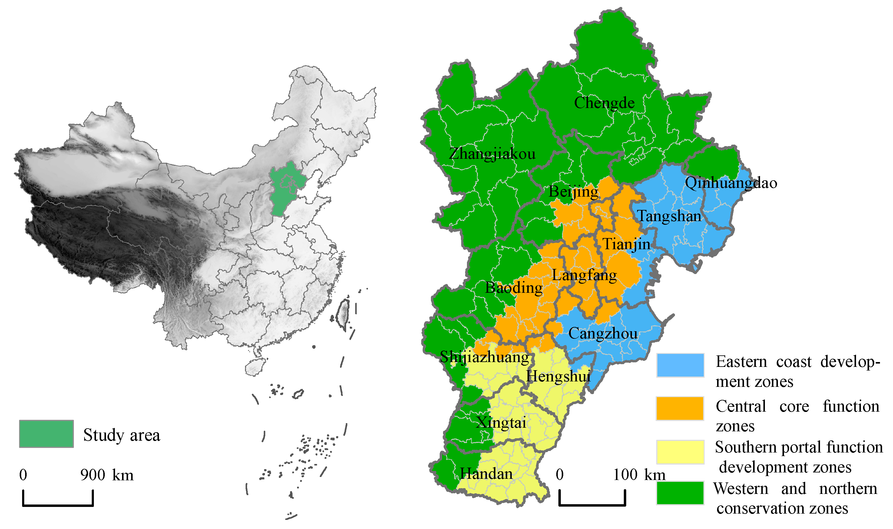
The Beijing–Tianjin–Hebei region includes two cities, namely Beijing and Tianjin, and a province, Hebei, which contain a total of 11 cities and 200 county-level administrative units. In 2015, the Chinese government issued the “Beijing–Tianjin–Hebei coordinated development planning outline”, which proposes to form four functional areas in combination with the natural and geographical environment, industrial development characteristics and relieving Beijing’s noncapital functions (Figure 1). Among them, the central core function zone is the core area leading the development of Beijing–Tianjin–Hebei, with a high degree of land development. The eastern coastal development zone focuses on the development of strategic emerging industries, and forms an industrial cluster coordinated with the ecological environment. The southern functional development zone mainly supplies agricultural and sideline products and controls the construction scale of cities and towns. The western and northern conservation zone is an area restricting industrialization and urbanization, which focuses on ecological protection, water conservation, and other functions.
The land area of this region is approximately 216,000 km², accounting for 2.3% of the area of the country. In 2016, the region had 110 million permanent residents, accounting for 8.1% of the population of the country; the GDP was 75.6 trillion, accounting for 10.2% of country’s GDP; the urbanization levels of the three zones were 86.5%, 82.9%, and 53.3%, respectively; and the densities of permanent population were 1324.1 people/km², 1328.5 people/km², and 398.0 people/km². The populations of both Beijing and Tianjin are thus highly concentrated. The deteriorating trend in the ecological environment in the region was manifested following the rapid development of the economy and rapid urbanization. The percentage of “Grade V” surface water and surface water deemed “inferior than Grade V” in the Beijing–Tianjin–Hebei region has reached 43% [37]; the percentage of water deemed “inferior than Grade V” is the highest among the major basins countrywide, and the pollution is the most severe. Along with the continuous advancement of a coordinated development strategy in the region, problems in the local ecological environment have caused widespread concern; the scarcity of water resources and serious water pollution have become a major bottleneck hindering regional green sustainable development.
2.2.2. Data Sources
COD and NH3-N are important indicators of water pollutions discharge, therefore, the spatial distribution of both will be studied here. Prior studies have explored the factors driving water pollution from different aspects such as level of urbanization, economic conditions, industrial structure, and technical level [8,38]. On the basis of prior research and the availability and representativeness of county-level administrative district data, a GWR model was built from the socioeconomic perspective. Table 1 presents the indicators selected.
The statistics for pollutants discharge of COD and NH3-N, and the social and economic data in both 2012 and 2016, all originated from Beijing Regional Statistical Yearbook, Tianjin Statistical Yearbook, Hebei Economic Yearbook, and statistical yearbooks of prefecture-level cities in Hebei published in 2013 and 2017. Due to administrative division adjustments, some county-level administrative units of the Beijing–Tianjin–Hebei region were merged during processing to unify the caliber of the data. Finally, 154 counties were obtained as research units. The data on administrative boundaries used in this study were obtained from the National Geomatics Center of China.
3. Results
3.1. Spatiotemporal Characteristics of the Discharge of Water Pollutants in the Beijing–Tianjin–Hebei Region
3.1.1. Emission Characteristics
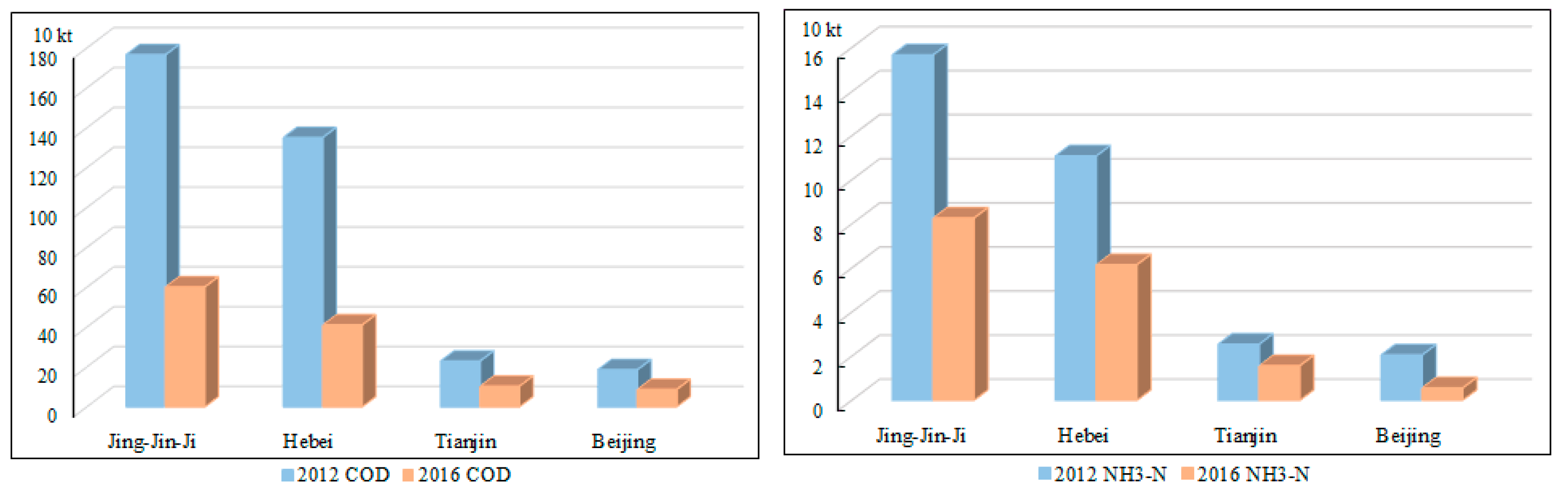
From 2012 to 2016, the quantity of pollutants discharged in the water environment of the Beijing–Tianjin–Hebei region exhibited a significant decreasing trend; the quantities of COD and NH3-N emissions dropped 65.9% and 47.2%, respectively. In 2012, the quantities of COD emissions in Beijing City, Tianjin City, and Hebei accounted for 10.6%, 13.0%, and 76.5% of COD emissions. In 2016, the share occupied by Hebei dropped to 68.4%, and for Beijing and Tianjin the share increased to 14.5% and 17.2%, respectively. Regarding COD, the emission reduction rate in Hebei was greatest (69.6%). The quantities of the emission of NH3-N changed from 13.1%, 16.2%, and 70.7% to 6.7%, 18.9%, and 74.3%, respectively. The emission reduction rate in Beijing was highest, reaching 72.8% (Figure 2).
3.1.2. Characteristics of Water Pollutants Discharge in Counties
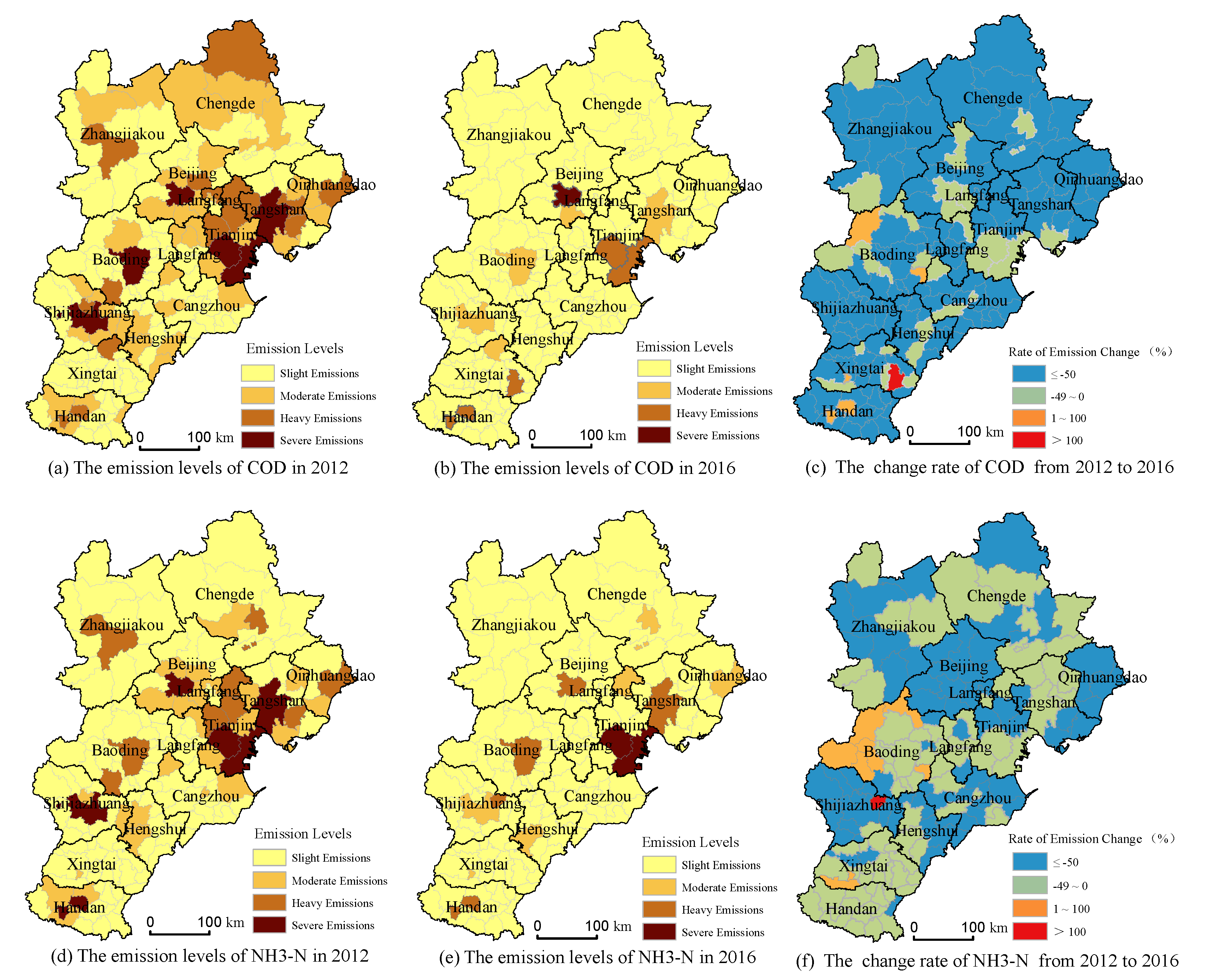
COD emissions in the Beijing–Tianjin–Hebei region in 2012 were characterized by concentrations in urban districts and their surrounding counties; a high emission zone of a wider scope was formed in the Bohai Rim region. The zones of harmful COD emissions were mainly city districts in Beijing, Tianjin, and Shijiazhuang and their surrounding counties, totaling 21 county units that jointly bore 41.6% of COD emission in the greater region. Low emission zones were scattered and distributed in the north of the Beijing–Tianjin–Hebei region as well as central and southern Hebei, accounting for 61% of the region’s total (Figure 3a). In 2016, more than 93% of Beijing–Tianjin–Hebei districts and counties were low emission zones. COD emissions in the counties had reduced substantially; only five districts and counties were deemed zones of high or extremely high COD emissions: a city district in each of Beijing, Tianjin, and Handan, Binhai New Area, and Wei County; the emissions were most concentrated in the city centers (Figure 3b). Notably, the quantities of emissions in Wei County, in city districts of Handan and Xingtai, and in Laiyuan County and Gaoyang County exhibited a rising trend (Figure 3c); in Wei County, emissions almost doubled.
In 2012, the zones of high or extremely high NH3-N emissions included city districts of Beijing, Tianjin, and Shijiazhuang and their surrounding districts and counties, which carried 40.2% of the quantity of NH3-N emissions in the Beijing–Tianjin–Hebei region. The low emission zones were mainly counties of Hebei Province, accounting for 74% of Beijing–Tianjin–Hebei counties (Figure 3d). In 2016, the NH3-N emissions in Beijing–Tianjin–Hebei counties dropped markedly; 91.6% of the counties were low emission zones, whereas only seven zones (including districts of Tianjin, Beijing, Tangshan, Baoding, and Handan) had high or extremely high emissions; and the scope was further narrowed to central urban areas (Figure 3e). From 2012 to 2016, the quantity of NH3-N emissions increased in nine counties, including Wuji County and Gaoyang County; the average increase exceeded 13.5%, and the increase of Wuji County exceeded 150% (Figure 3f).
3.2. Characteristics of the Spatiotemporal Evolution of Water Pollutants Discharge in the Beijing–Tianjin–Hebei Region
3.2.1. Spatial Correlation Analysis
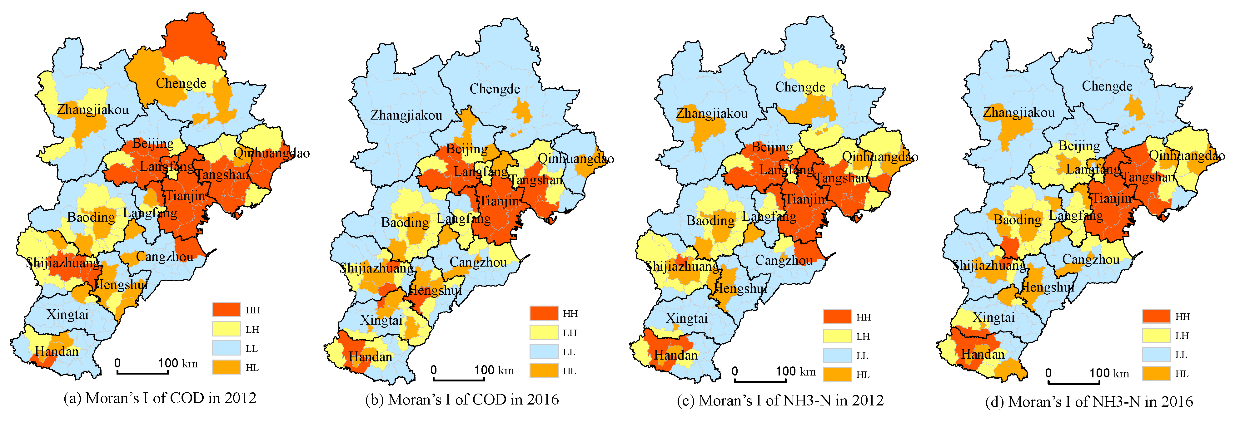
The Moran’s I values of the quantities of COD and NH3-N emissions were significantly positive (Table 2), indicating a significant and positive spatial correlation with the discharge of water pollutants in Beijing–Tianjin–Hebei counties, which was spatially manifested as the agglomeration and distribution of zones of high-value or low-value pollutant discharges. The Moran’s I value of the COD emissions of 2016 dropped from that of 2012, indicating that the spatial correlation of COD emissions decreased during the study period, and the trend of concentrated pollutant emissions became weaker. The Moran’s I value of NH3-N emissions in 2016 increased obviously, indicating that the spatial correlation became stronger and the trend of concentrated pollutant emissions was enhanced.
Figure 4 is a two-dimensional visualization of a Moran scatter plot. The counties whose COD emissions of 2012 and 2016 were in the first and third quadrants (HH and LL) accounted for 66.9% and 59.1% of all counties; the positive correlation in COD emissions was significant. The HH agglomeration zones were mainly situated in the Bohai Rim region, but the distribution area was narrowed; agglomeration zones with high emissions in southern Hebei showed an expanding trend; the LL agglomeration zones were mainly distributed in Zhangjiakou, Chengde, Baoding, Cangzhou and Xingtai regions; and the overall number remained unchanged, and the spatial distribution was more concentrated (Figure 4a,b). The percentages of counties whose NH3-N emissions of 2012 and 2016 were in the first and the third quadrants (HH and LL) were 65.6% and 61.7%; the counties of HH agglomerations were distributed mainly in the Beijing–Tianjin–Tangshan region. The number dropped, and expansion was seen in southern Hebei. The LL agglomeration zones were distributed mainly in the Zhangjiakou, Chengde, and Xingtai regions, and the scope of the distribution was wider (Figure 4c,d).
3.2.2. Spatiotemporal Transition Analysis
From 2012 to 2016, the most pervasive type of transitions of COD and NH3-N in Beijing–Tianjin–Hebei counties was Type D (no transition occurred in the counties and the surrounding areas; Figure 4); this type of COD transition existed in 59.1% of counties, and this type of NH3-N transition existed in 74.7% of counties (i.e., the spatial stability of each was 0.591 and 0.747); and the spatial distribution of water pollutants in Beijing–Tianjin–Hebei counties was characterized by high stability. Both Type A and Type B COD transitions occurred in 27 counties; a Type C transition occurred in 9 counties. Both Type A and Type B NH3-N transitions occurred in 19 counties; a Type C transition occurred in only 1 county. The probability of a transition occurring in neighboring regions was higher than that in the counties; the spatiotemporal cohesion of the water pollutants in Beijing–Tianjin–Hebei counties was higher than the spatiotemporal fluidity, indicating strong spatial locking.
3.2.3. Spatial Pattern Analysis
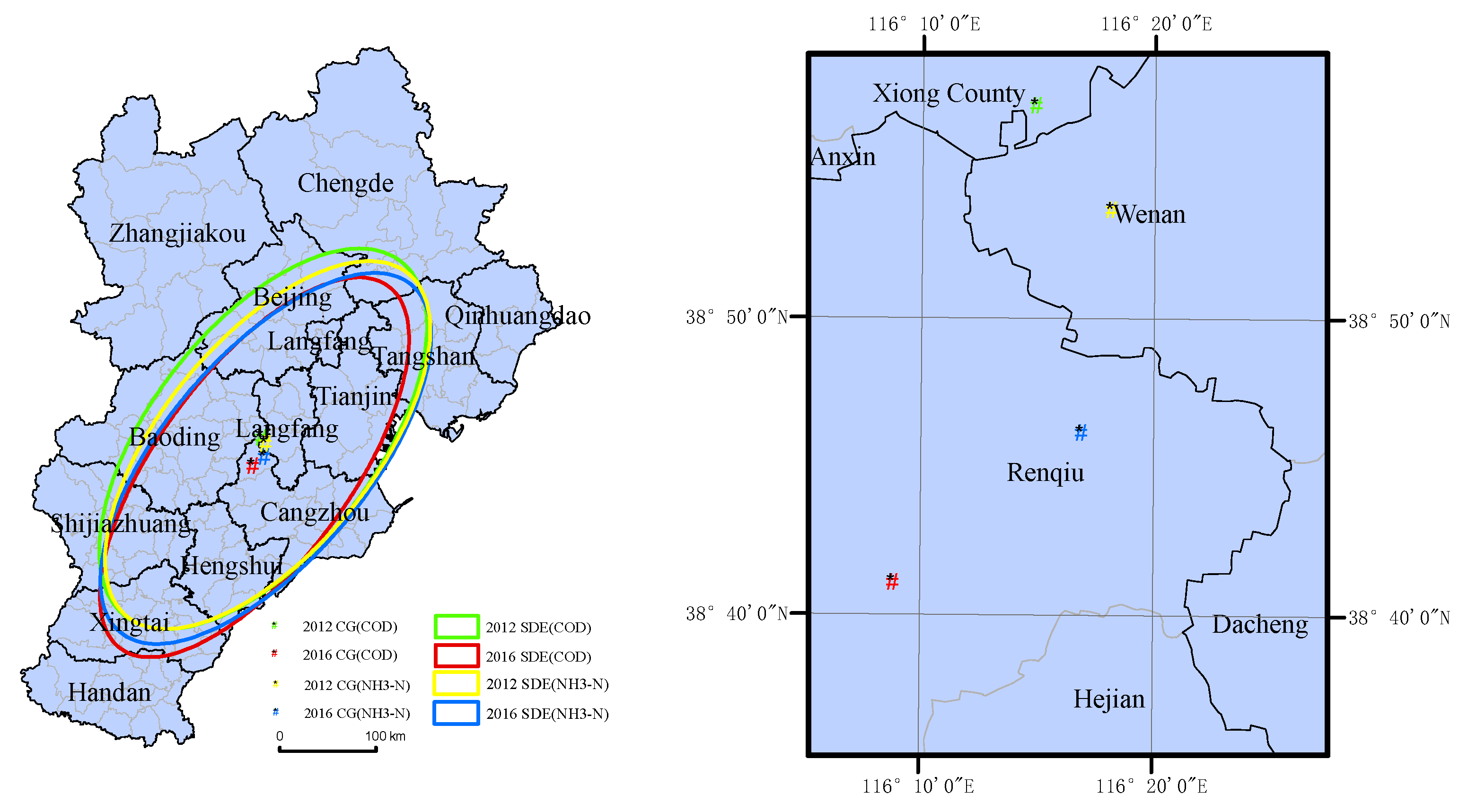
From 2012 to 2016, the centers of gravity of the discharge of water pollutants in the Beijing–Tianjin–Hebei region were distributed at 38°41′–38°57′ N and 116°9′–116°18′ E, the intersection of the cities of Baoding, Langfang, and Cangzhou; the center of gravity tended to move south. Additionally, from 2012 to 2016, the centers of gravity of COD and NH3-N both moved in the northeast–southwest direction; the center of gravity of COD moved from Xiong County to inside Renqiu City over a distance of 31,000 m, and the distance of deflection was longer. The center of gravity of NH3-N moved from Wen’an County to Renqiu City over a distance of 14,000 m; the distance of deflection was shorter. The spatial distribution of water pollutants discharge in Beijing–Tianjin–Hebei remained in the pattern of a northeast–southwest distribution. Regarding the COD standard deviational ellipse, the standard deviation of the short axis decreased from 116.5 km to 99.6 km, and the standard deviation of the long axis increased from 233.2 km to 233.9 km. Regarding NH3-N, the standard deviation of the short axis decreased from 109.2 km to 105.6 km; the standard deviation of the long axis increased from 230.2 km to 235.4 km, indicating a notable converging tendency of water pollutants discharge in the northwest to southeast direction and a dispersing tendency in the northeast to southwest direction (Figure 5).
3.3. Analysis of the Factors Driving the Discharge of Water Pollutants in Beijing–Tianjin–Hebei Counties
In 2016, the center of gravity of water pollution in the Beijing–Tianjin–Hebei region obviously moved south. The discharge of water pollutants and the resultant phenomenon of water pollution in the region and particularly in Hebei counties remained acute; it was imperative to determine the crucial factors of influence for the discharge of water pollutants and to react proactively.
3.3.1. Estimation Results of OLS Model
Examination results of the OLS regression (Table 3) revealed that the regression variance of the two water pollutant models involved no redundancy or multicollinearity (VIF < 7.5). Jarque–Bera and Koenker (BP) tests both rejected the null hypothesis; the coefficients of determination R2 reflected the weaker explanatory power (approximately 45% and 54%) of OLS model regression, and the introduction of the GWR model was required to examine the spatial heterogeneity of the driving factors. The results of GWR model testing proved that the model’s AICc value was significantly less than that of the OLS model; calibrated R2 values increased by 12.2% and 15.5% from those of the OLS model.
The values of the factors’ regression coefficients indicated that PGDP, UR, and IPA had significant and positive effects on driving water pollutants discharge in Beijing–Tianjin–Hebei counties. Increases in the three indicators would significantly increase the amount of water pollutants discharge in these counties. The PGDP indicator’s driving coefficient exceeded 0.5. The ER factors had a significant effect on reducing pollutant emissions; increasing the intensity of ER had greater effect on reducing NH3-N emission reduction. The regression coefficients of the IS and DC indicators were negative, but their significance levels were less strong; the directions of action of both in relation to the water pollutants in Beijing–Tianjin–Hebei counties remained uncertain.
3.3.2. Analysis of the Spatial Heterogeneity of the Driving Factors
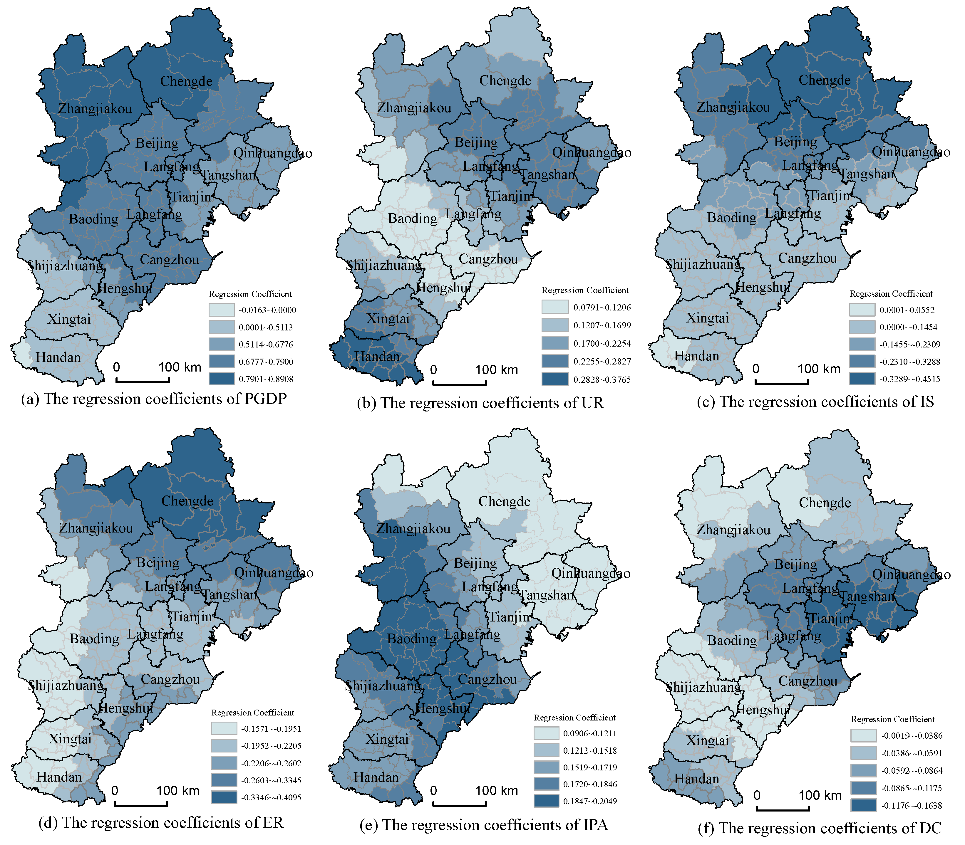
Spatial distribution graphs of the regression coefficients of the GWR models of COD and NH3-N (Figure 6 and Figure 7) were generated to facilitate the analysis of the spatial heterogeneity of the driving factors. In terms of COD emission, the direction of action of the PGDP and IS factors involved spatial heterogeneity; the directions of action of other factors in the Beijing–Tianjin–Hebei region were uniform. The regression coefficient of the PGDP was positive in all counties except She County in the southwestern part of the region; the effect intensity exhibited a gradually decreasing trend from the northwest to the southeast. The regression coefficient of IS in a few counties in southwestern Beijing–Tianjin–Hebei was positive, and those in other counties were negative. The effect intensity gradually decreased from north to south. The regression coefficients of UR and IPA in the total area were positive, but the effect intensity was exactly the opposite. The effect intensity of UR gradually decreased from the northeastern and southwestern areas toward the central Beijing–Tianjin–Hebei region, whereas IPA’s effect intensity gradually decreased from the vast central Beijing–Tianjin–Hebei area outward. The regression coefficients of the ER and DC factors for the entire area were negative. The effect intensity of ER gradually decreased from the north to the west of Beijing–Tianjin–Hebei; ER’s effect on reducing emissions from the discharge of water pollutants in northern Beijing–Tianjin–Hebei was the most significant. The effect intensity of DC was greatest in the Bohai Rim region, and COD emissions in the region represented a clearer core-edge structure (Figure 6).
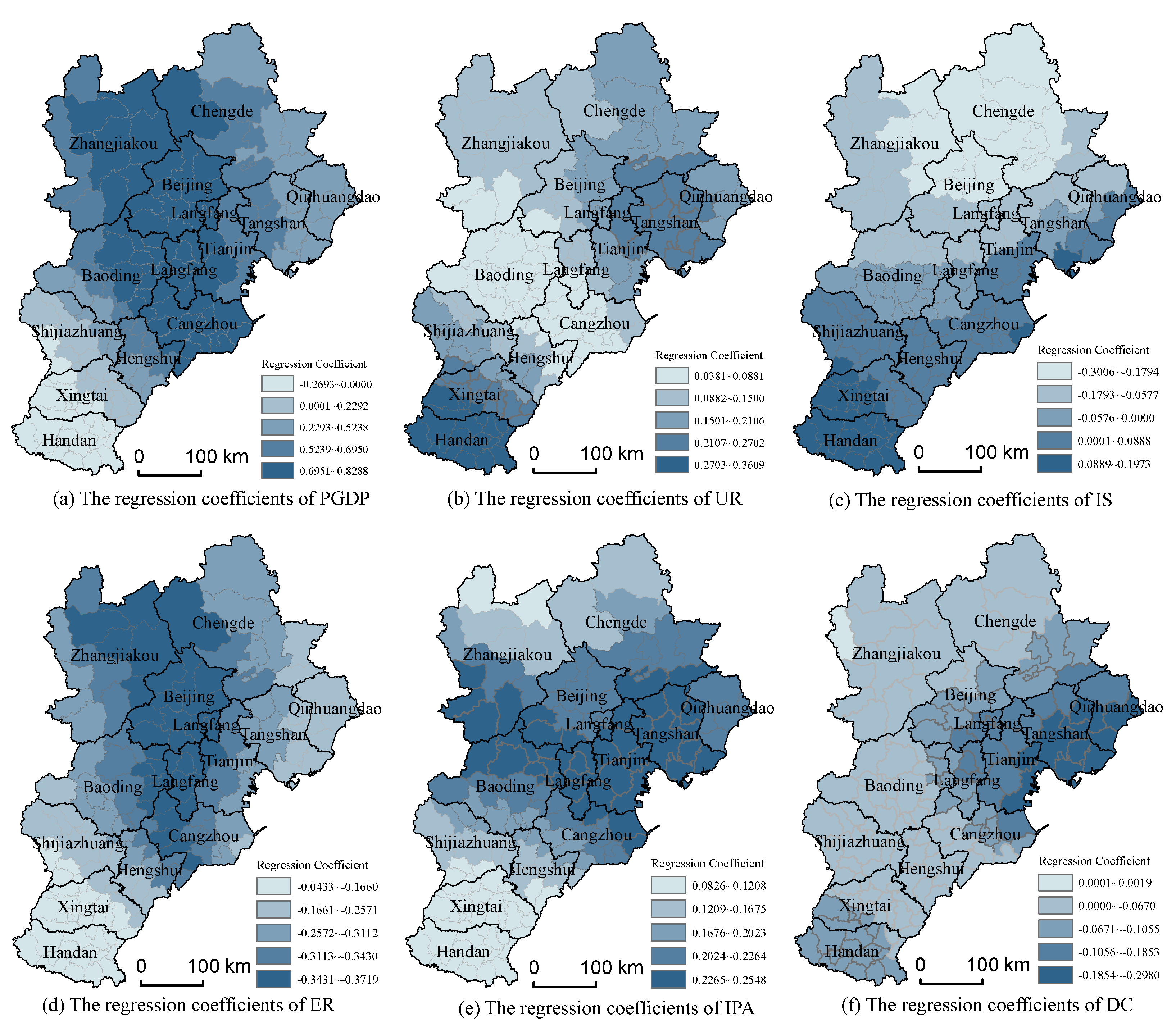
Regarding NH3-N emissions, the directions of action of the PGDP, IS, and DC factors involved spatial heterogeneity; the directions of action of other factors in the Beijing–Tianjin–Hebei Region were uniform. Except in the southern Beijing–Tianjin–Hebei counties, the regression coefficients of the PGDP factor were positive. The effect intensity gradually decreased starting from around the cities of Zhangjiakou, Beijing, Langfang, and Cangzhou to the other two sides. With the northern part of Baoding as the boundary, in the region to its north, IS indicated negative driving; in the region to its south, IS indicated positive driving and the effect intensity gradually decreased from the boundary toward both sides. The regression coefficient of DC in Shangyi County in the Beijing–Tianjin–Hebei region was positive; it represented the phenomenon of “refuge from pollution” in the region. The regression coefficients of the DC factors in other Beijing–Tianjin–Hebei counties were positive; similar to the case of COD, the effect intensities in the northeastern Beijing–Tianjin–Hebei counties were higher. The regression coefficients of the UR and IPA factors in the total area were positive, but the effect intensities differed more greatly. UR’s effect intensity gradually decreased from the northeast and the southern Beijing–Tianjin–Hebei regions toward the central area; IPA’s effect intensity gradually decreased from around Tangshan, Tianjin, Langfang, and Baoding toward both sides; and the effect intensity in southern Beijing–Tianjin–Hebei was weakest. ER’s regression coefficient for the entire area was negative; the effect intensity gradually decreased from around Zhangjiakou, Beijing, Langfang, and Cangzhou toward both sides; and the effect for emission reduction in Beijing and its surrounding area was the most significant.
4. Conclusions and Policy Suggestions
From 2012 to 2016, the pollutant discharge in the water environment of the Beijing–Tianjin–Hebei region dropped significantly; the quantities of COD and NH3–N emissions dropped 65.9% and 47.2%, respectively; and the acute situation of water pollution was alleviated. The reduction of COD emissions was largest in Hebei Province; the reduction of NH3-N emissions was largest in Beijing. In 2016, the number of high water pollution zones dropped significantly and over 91% of the counties in the region were ranked as low-emission. However, the intersections of administrative boundaries continued to face the pressure of considerable pollutant emissions, which is consistent with the authors’ previous research results [39].
The results showed that, the water pollutants discharge in the Beijing–Tianjin–Hebei region had a significant and positive spatial correlation, this conclusion is consistent with that of Gao [19]. The HH agglomeration zones were mainly distributed in the Bohai Rim region and exhibited a decreasing trend, but the scope of the HH agglomeration zones in southern Hebei was expanded. The LL agglomeration zones were mainly distributed in the Zhangjiakou, Chengde, and XingTai regions. During the study period, the center of gravity of water pollutants in Beijing–Tianjin–Hebei deflected southwest, representing a stronger converging trend in the northwest–southeast direction and a dispersing trend in the northeast–southwest direction. The spatiotemporal cohesion of water pollutants was greater than their spatiotemporal fluidity, with strong spatial locking.
PGDP, UR, and IPA were the significant and positive driving factors for the discharge of water pollutants in the Beijing–Tianjin–Hebei counties. Increases in these three indicators would aggravate the regional water pollutants discharge. ER had a significant effect in reducing the emission of pollutants and its effect on reducing NH3-N emissions was greater. The driving effects of IS and DC were probably not significant. Both the direction of action and the effect intensity of PGDP, IS, and DC in relation to the discharge of water pollutants in Beijing–Tianjin–Hebei counties represented significant spatial heterogeneity; the effect intensity of UR, ER, and IPA exhibited spatial heterogeneity.
The spatial heterogeneity of the driving factors identified in the study along with the spatial development pattern of the Beijing–Tianjin–Hebei region allow the following policy suggestions.
First, the effect intensity of factors in the coastal development zone in the east was more balanced, and the driving intensities of UR and DC were greater. Governments should focus on the high-intensity industrial development in the zone and the coastal location characteristics, constrain the development of heavy chemical industries, adequately relieve demographic and economic factors in the urban center, optimize the layout of urban and industrial spaces, and prevent over-concentrations of demographic and economic factors.
Second, strong multi-factor (PGDP, UR, and IPA) effects were manifested in the central core functional zone. The key was controlling both urban life sources and agricultural sources; the government should approach through regulating the speed and intensity of economic development, strengthening the classification management of waste originated in urban life and control of the totality of pollution, enhancing the supervision of agricultural production (particularly suburban agriculture), and encouraging green agricultural production through tax subsidies to gradually reduce the discharge of pollutants originated from agricultural sources.
Third, the strong driving of two factors (UR and IPA) was manifested in the functional development zone in the south. The zone is a crucial site undertaking the “relief of noncapital functions” of Beijing and a major area of agricultural product supply in the Beijing–Tianjin–Hebei region; emphasis should be placed on expanding infrastructure in the regional environmental, building robust agricultural wastewater treatment plants, enhancing the supervision of the environments of urban border regions, and adequately undertaking population and industries by improving the comprehensive carrying capacity of the region.
Last, strong driving of multi-factors (PGDP, IS, ER, IPA, and UR) was manifested in the ecological conservation zone in the northwest. This zone is a vital water source area in the Beijing–Tianjin–Hebei region; the government should limit large-scale, high-intensity construction for urbanization and industrialization in the region and, on the basis of implementing the boundaries and intensity of urban development, appropriately tighten the development and construction policies for this type of region to maximize the effect of environmental regulations and cleaner production on emission reductions.
5. Study limitations and Future Prospects
Although major results were obtained in the study, the following crucial challenges remain to be resolved by future research:
- Since legal and financial conditions stand in the way, change is not always possible or proceeds at an insufficient pace, the implementation effect of the policy will be obvious in a long time. If we can use longer or more periods of data, we will get better results. Due to the limitation of statistics of county units, unfortunately, this study only analyzed the data of 2012 and 2016. It is expected that more years of data will be used to analyze this phenomenon in the future.
- This paper analyzed the influencing factors of water pollution discharge from social and economic perspectives. In fact, climate and hydrological conditions are also important factors affecting the pattern of water pollution discharge. Therefore, the follow-up research should fully consider the climate and hydrological conditions. In addition, according to the current research [20], the differences in policy intensity of different pollutant discharge in industrial sectors and main functional zones also have an important impact on pollutants discharge, so both of them should be considered as the influencing factors of analysis when the data can be collected.
Author Contributions
Conceptualization, H.L.; Investigation, Q.R.; Methodology, H.L.; Software, Q.R.; Supervision, H.L.; Writing—review and editing, Q.R. All authors have read and agreed to the published version of the manuscript.
Funding
The work in this study was supported by the Social Science foundation of Jiangsu, China (20EYC010).
Institutional Review Board Statement
Not applicable.
Informed Consent Statement
Not applicable.
Data Availability Statement
The data presented in this study are available on request from the corresponding author.
Acknowledgments
Authors thank the editor and anonymous reviewers for their insightful comments on an earlier version of the manuscript.
Conflicts of Interest
The authors declare no conflict of interest.
References
- Finance Sina. Environmental Governance Becomes a Hot Topic of the National People’s Congress and the Chinese Political Consultative Conference (NPC & CPPCC): Green Water and Green Mountains are Necessary. 2015. Available online: http://finance.sina.com.cn/china/20150304/014221637280.shtml (accessed on 4 March 2015).
- Hu, Y.; Cheng, H. Water pollution during China’s industrial transition. Environ. Dev. 2013, 8, 57–73. [Google Scholar] [CrossRef]
- Ji, X.; Zhang, W.; Jiang, M.; He, J.; Zheng, Z. Black-odor water analysis and heavy metal distribution of Yitong River in Northeast China. Water Sci. Technol. 2017, 76, 2051–2064. [Google Scholar] [CrossRef]
- Larsen, T.A.; Hoffmann, S.; Lüthi, C.; Truffer, B.; Maurer, M. Emerging solutions to the water challenges of an urbanizing world. Science 2016, 352, 928–933. [Google Scholar] [CrossRef] [PubMed]
- Ilyas, M.; Ahmad, W.; Khan, H.; Yousaf, S.; Yasir, M.; Khan, A. Environmental and health impacts of industrial wastewater effluents in Pakistan: A review. Rev. Environ. Health 2019, 34, 171–186. [Google Scholar] [CrossRef] [PubMed]
- Noguerol-Arias, J.; Rodríguez-Abalde, A.; Romero-Merino, E.; Flotats, X. Determination of chemical oxygen demand in heterogeneous solid or semisolid samples using a novel method combining solid dilutions as a preparation step followed by optimized closed reflux and colorimetric measurement. Anal. Chem. 2012, 84, 5548–5555. [Google Scholar] [CrossRef]
- Wang, H.; Zhong, S.; He, Y.; Song, G. Molecular sieve 4A–TiO2–K2Cr2O7 coexisted system as sensor for chemical oxygen demand. Sens. Actuators B. 2011, 160, 189–195. [Google Scholar] [CrossRef]
- Li, L.G.; Zhang, P.Y.; Liu, W.X.; Li, J.; Wang, L.F. Spatial-temporal evolution characteristics and influencing factors of county-scale environmental pollution in Jilin Province, Northeast China. Chin. J. Appl. Ecol. 2019, 30, 2361–2370. [Google Scholar]
- Canals, A.; Del Remedio Hernandez, M. Ultrasound-assisted method for determination of chemical oxygen demand. Anal. Bioanal. Chem. 2002, 374, 1132–1140. [Google Scholar] [CrossRef]
- Zhang, P.; Yang, D.; Zhang, Y.; Li, Y.; Liu, Y.; Cen, Y.; Zhang, W.; Geng, W.; Rong, T.; Liu, Y. Re-examining the drive forces of China’s industrial wastewater pollution based on GWR model at provincial level. J. Clean. Prod. 2020, 262, 1–14. [Google Scholar] [CrossRef]
- Wang, H.; Luan, W.; Kang, M. COD pollution load of social and economic activities in liaohe river basin, China. Geog. Res. 2013, 32, 1802–1813. [Google Scholar]
- Zhao, X.W.; Shen, Z.L.; Zhang, H.Z.; Feng, H.B.; Liu, G.H.; Xu, J.J.; Zhao, N. Study on the COD Emission Trends and the Reduction Measures in Hebei Province. South North Water Transf. Water Sci. Technol. 2010, 8, 65–67. [Google Scholar]
- Maringanti, C.; Chaubey, I.; Popp, J. Development of a multiobjective optimization tool for the selection and placement of best management practices for nonpoint source pollution control. Water Resour. Res. 2009, 45, 1–15. [Google Scholar] [CrossRef] [Green Version]
- Cai, J.J.; Varis, O.; Yin, H. China’s water resources vulnerability: A spatio-temporal analysis during 2003–2013. J. Clean. Prod. 2017, 142, 2901–2910. [Google Scholar] [CrossRef]
- Zhou, K.; Fan, J. Regional disparity of environmental pollution source and its socio-economic influencing factors: Based on the cross-section data of 339 cities at prefecture level or above in China. Acta Geog. Sin. 2016, 71, 1911–1925. [Google Scholar]
- Lu, Y.; Wu, S.; Zhu, J.H.; Jia, J.L. Analysis on effect decomposition of industrial COD emission. Procedia Environ. Sci. 2012, 13, 2197–2209. [Google Scholar] [CrossRef] [Green Version]
- Wang, C.; Sun, Q.; Jiang, S.; Wang, J.K. Evaluation of Pollution Source of the Bays in Fujian Province. Procedia Environ. Sci. 2011, 10, 685–690. [Google Scholar]
- Zhao, X.F.; Huang, X.J.; Zhang, X.Y.; Zhu, D.M.; Lai, L.; Zhong, T.Y. Application of spatial autocorrelation analysis to the COD, SO2 and TSP emission in Jiangsu Province. Environ. Sci. 2009, 30, 1580–1587. [Google Scholar]
- Gao, S.; Wei, Y.H.; Chen, W.; Zhao, H.X. Study on spacial-correlation between water pollution and industrial agglomeration in the developed region of China: A case study of Wuxi City. Geog. Res. 2011, 30, 902–912. [Google Scholar]
- Yu, H.; Zhong, J.; Liu, S.Q.; Yang, D.W. The coupling characteristics between polluting industrial agglomeration and water pollution discharge in Zhangjiakou. J. Nat. Resour. 2020, 35, 1416–1424. [Google Scholar]
- Ma, H.L.; Nie, X.; Li, D. Study on Water Pollution Governance Effect of Taihu Basin: Based on Pollution Index Analysis. Ecol. Econ. 2014, 30, 183–189. [Google Scholar]
- Zhou, K.; Wu, J.X.; Qian, Z.D.; Fan, J.; Wang, Q. Spatial effects on emission reduction of water pollutants and its driving forces in Yangtze River Economic Belt. China Environ. Sci. 2020, 40, 885–895. [Google Scholar]
- Bai, L.; Sun, Y.Y.; Zhao, X.T.; Qiao, Q.; Li, X.Y.; Zhou, X.Y. Discharge Characteristics and Pollution Aggregation Pattern of Water Pollution in Yellow River Basin. Res. Environ. Sci. 2020, 33, 2683–2694. [Google Scholar]
- He, L.P.; Zhang, X.; Chen, S. An Analysis of Water Pollution Situation and Its Main Causes in Pearl River Basin. Environ. Sci. Surv. 2012, 31, 24–28. [Google Scholar]
- Wen, Q.; Chen, X.; Shi, Y.; Ma, J.; Zhao, Q. Analysis on Composition and Pattern of Agricultural Nonpoint Source Pollution in Liaohe River Basin, China. Procedia Environ. Sci. 2011, 8, 26–33. [Google Scholar] [CrossRef] [Green Version]
- Liu, X.; Li, G.; Liu, Z.; Guo, W.; Gao, N. Water pollution characteristics and assessment of lower reaches in Haihe River Basin. Procedia Environ. Sci. 2010, 2, 199–206. [Google Scholar] [CrossRef] [Green Version]
- Yue, Y.; Cheng, H.G.; Yang, S.T.; Hao, F.H. Integrated assessment of non-point source pollution in Songhuajiang river basin. Sci. Geog. 2007, 27, 231–236. [Google Scholar]
- Amaya, F.L.; Gonzales, T.A.; Hernandez, E.C.; Luzano, E.V.; Mercado, N.P. Estimating Point and Non-Point Sources of Pollution in Biñan River Basin, the Philippines. Apcbee Procedia 2012, 1, 233–238. [Google Scholar] [CrossRef] [Green Version]
- Fang, C.L. Progress and the future direction of research into urban agglomeration in China. Acta Geog. Sin. 2014, 69, 1130–1144. [Google Scholar]
- Wang, Z.B.; Li, J.X.; Liang, L.W. Spatio-temporal evolution of ozone pollution and its influencing factors in the Beijing-Tianjin-Hebei Urban Agglomeration. Environ. Pollut. 2020, 256, 113419.1–113419.11. [Google Scholar] [CrossRef] [PubMed]
- Ren, W.; Zhong, Y.; Meligrana, J.; Anderson, B.; Watt, W.E.; Chen, J.; Leung, H.L. Urbanization, land use, and water quality in Shanghai: 1947–1996. Environ. Int. 2003, 29, 649–659. [Google Scholar] [CrossRef]
- Rey, S.J.; Janikas, M.V. Space-Time Analysis of Regional Systems. Geog. Anal. 2006, 38, 67–86. [Google Scholar] [CrossRef]
- Getis, A.; Ord, J.K. The Analysis of Spatial Association by Use of Distance Statistics. Geog. Anal. 2010, 24, 189–206. [Google Scholar] [CrossRef]
- Rey, S.J. Spatial Empirics for Economic Growth and Convergence. Geog. Anal. 2010, 33, 195–214. [Google Scholar] [CrossRef]
- Lefever, D.W. Measuring Geographic Concentration by Means of the Standard Deviational Ellipse. Am. J. Sociol. 1926, 32, 88–94. [Google Scholar] [CrossRef]
- Fotheringham, A.S.; Charlton, M.E.; Brunsdon, C. Geographically Weighted Regression: A Natural Evolution of the Expansion Method for Spatial Data Analysis. Environ. Plann. A 1998, 30, 1905–1927. [Google Scholar] [CrossRef]
- Wang, K. Coordinated development of The Beijing-Tianjin-Hebei Region under the new Normal. Small Cities Towns. 2015, 31–34. [Google Scholar]
- Jin, W.; Zhang, H.Q.; Liu, S.S.; Zhang, H.B. Technological innovation, environmental regulation, and green total factor efficiency of industrial water resources. J. Clean. Prod. 2019, 211, 61–69. [Google Scholar] [CrossRef]
- Zhou, K.; Li, H.; Shen, Y. Spatiotemporal patterns and driving factors of environmental stress in Beijing-Tianjin-Hebei region: A county-level analysis. Acta Geog. Sin. 2020, 75, 1934–1947. [Google Scholar]
Figure 1.
Overview map of the Beijing–Tianjin–Hebei region.

Figure 2.
Schematic of water pollutant discharge in Beijing City, Tianjin City, and Hebei Province in 2012 and 2016.
Figure 2.
Schematic of water pollutant discharge in Beijing City, Tianjin City, and Hebei Province in 2012 and 2016.

Figure 3.
Characteristics of spatiotemporal emissions and water pollutants change in Beijing–Tianjin–Hebei counties from 2012 to 2016.
Figure 3.
Characteristics of spatiotemporal emissions and water pollutants change in Beijing–Tianjin–Hebei counties from 2012 to 2016.

Figure 4.
Moran’s I scatter plot of the discharge of water pollutants in the Beijing–Tianjin–Hebei Region.
Figure 4.
Moran’s I scatter plot of the discharge of water pollutants in the Beijing–Tianjin–Hebei Region.

Figure 5.
Center of gravity (CG) of water pollutants discharge in the Beijing–Tianjin–Hebei region and standard deviational ellipse (SDE).
Figure 5.
Center of gravity (CG) of water pollutants discharge in the Beijing–Tianjin–Hebei region and standard deviational ellipse (SDE).

Figure 6.
Spatial distribution graph of the regression coefficients of driving factors for COD.

Figure 7.
Spatial distribution graph of the regression coefficients of driving factors for NH3-N.


Table 1.
Model indicators and definitions.
| Indicator | Code | Definition of Variable |
|---|---|---|
| Dependent variable | COD | Quantity of COD emissions (10,000 tons) |
| NH3-N | Quantity of NH3-N emissions (10,000 tons) | |
| Level of economic development | PGDP | GRP per capita (yuan) |
| Level of urbanization | UR | Proportion of urban population in total population (%) |
| Industrial structure | IS | Proportion of the added value of secondary industry in GDP (%) |
| Environmental regulations | ER | Proportion of governance costs for water pollutants in GDP (%) |
| Agricultural production input | IPA | Fertilizer consumption (purity) (tons) |
| Distance attenuation effect | DC | Distance between the county center and the city center (1000 m) |
Table 2.
Expected Moran’s I values of water pollutants in the Beijing–Tianjin–Hebei region.
| 2012 | 2016 | |||
|---|---|---|---|---|
| COD | NH3-N | COD | NH3-N | |
| Moran’s I | 0.1666 | 0.1592 | 0.1309 | 0.1933 |
| z-score | 3.6114 | 3.6328 | 2.9777 | 4.4142 |
| p-value | 0.0003 | 0.0003 | 0.0029 | 0.0000 |
Table 3.
Results of OLS model for the factors driving water pollutants discharge in Beijing–Tianjin–Hebei counties.
Table 3.
Results of OLS model for the factors driving water pollutants discharge in Beijing–Tianjin–Hebei counties.
| Driving Factors | COD | NH3-N | ||||||
|---|---|---|---|---|---|---|---|---|
| Coefficient | StdError | T-Statistic | VIF | Coefficient | StdError | T-Statistic | VIF | |
| Intercept | 0.036 | 0.046 | 0.777 | — | −0.001 | 0.035 | −0.02 | — |
| PGDP | 0.566 *** | 0.102 | 5.534 | 2.062 | 0.550 *** | 0.081 | 6.795 | 2.219 |
| UR | 0.200 *** | 0.062 | 3.203 | 2.016 | 0.152 *** | 0.047 | 3.218 | 1.977 |
| IS | −0.129 * | 0.066 | −1.971 | 1.205 | −0.037 | 0.021 | −0.73 | 1.231 |
| ER | −0.198 *** | 0.066 | −3.022 | 1.171 | −0.265 *** | 0.059 | −4.482 | 1.286 |
| IPA | 0.152 *** | 0.052 | 2.943 | 1.036 | 0.165 *** | 0.040 | 4.170 | 1.042 |
| DC | −0.066 | 0.052 | −1.268 | 1.339 | −0.069 * | 0.039 | −1.761 | 1.317 |
| Model | Adjusted R² | AICc | Koenker (BP) | Jarque–Bera | Adjusted R² | AICc | Koenker (BP) | Jarque–Bera |
| Diagnosis | 0.453 | −237.29 | 38.439 ** | 1092.948 ** | 0.542 | −320.299 | 83.947 ** | 434.023 ** |
Note: *** p < 0.01, ** p < 0.05, * p < 0.1.
Publisher’s Note: MDPI stays neutral with regard to jurisdictional claims in published maps and institutional affiliations. |
© 2021 by the authors. Licensee MDPI, Basel, Switzerland. This article is an open access article distributed under the terms and conditions of the Creative Commons Attribution (CC BY) license (https://creativecommons.org/licenses/by/4.0/).
Share and Cite
MDPI and ACS Style
Ren, Q.; Li, H. Spatiotemporal Effects and Driving Factors of Water Pollutants Discharge in Beijing–Tianjin–Hebei Region. Water 2021, 13, 1174. https://doi.org/10.3390/w13091174
AMA Style
Ren Q, Li H. Spatiotemporal Effects and Driving Factors of Water Pollutants Discharge in Beijing–Tianjin–Hebei Region. Water. 2021; 13(9):1174. https://doi.org/10.3390/w13091174
Chicago/Turabian StyleRen, Qilong, and Hui Li. 2021. "Spatiotemporal Effects and Driving Factors of Water Pollutants Discharge in Beijing–Tianjin–Hebei Region" Water 13, no. 9: 1174. https://doi.org/10.3390/w13091174
Note that from the first issue of 2016, this journal uses article numbers instead of page numbers. See further details here.