
Machine Learning Modeling of Climate Variability Impact on River Runoff


1
Institute for Agricultural and Forest Environment, Polish Academy of Sciences, 60-809 Poznan, Poland
2
Institute of Computing Science, Poznań University of Technology, 60-965 Poznan, Poland
3
Center for Artificial Intelligence and Machine Learning (CAMIL), 60-965 Poznan, Poland
*
Author to whom correspondence should be addressed.
Water 2021, 13(9), 1177; https://doi.org/10.3390/w13091177
Submission received: 12 February 2021
/
Revised: 21 April 2021
/
Accepted: 22 April 2021
/
Published: 24 April 2021
(This article belongs to the Section Hydrology)
Abstract
:The hypothesis of this study was one of existence of spatially organized links between the time series of river runoff and climate variability indices, describing the oscillations in the atmosphere–ocean system: ENSO (El Niño–Southern Oscillation), PDO (Pacific Decadal Oscillation), AMO (Atlantic Multidecadal Oscillation), and NAO (North Atlantic Oscillation). The global river flow reconstructions (ERA-20-CM-R) for 18 study areas on six continents and climate variability indices for the period 1901–2010 were used. The split-sample approach was applied, with the period 1901–2000 used for training and 2001–2010 used for testing. The quality measures used in this paper were mean absolute error, dynamic time warping, and top extreme events error. We demonstrated that a machine learning approach (convolution neural network, CNN) trained on climate variability indices can model the river runoff better than the long-term monthly mean baseline, both in univariate (per-cell) and multivariate (multi-cell, regionalized) settings. We compared the models to the baseline in the form of heatmaps and presented results of ablation experiments (test time ablation, i.e., jackknifing, and training time ablation), which suggested that ENSO is the primary determinant among the considered indices.
1. Introduction
Destructive floods kill, on average, thousands of people worldwide per year, and cause material loss of the order of tens of billions to hundreds of billions of USD [1]. There have been many reports on dramatic deluges, particularly in less developed countries. Very high flood risk, in terms of both percentage of national population and national GDP affected, has been found to exist in Southeast Asia (Vietnam, Cambodia, Bangladesh) [2]. However, large floods have been also reported in recent years in large countries of Asia—China, India, and Pakistan, as well as in Africa, the Americas, and Australia. Moreover, in Europe, many destructive floods have been recorded in recent decades, with the costliest one, in August 2002, affecting Germany, Austria, and the Czech Republic in particular. Despite all the progress made in monitoring, forecasting, and safeguarding, there is no place on earth where this challenge has been definitely solved [3].
It is well known that flood risk has been increasing with time in virtually all spatial scales [1,2], mainly due to increasing exposure and vulnerability of people and property. However, there are huge gaps in understanding of changes in flood hazard and flood risk. Increase of frequency and amplitude of intense precipitation is expected in warmer climates. However, no general, ubiquitous, and statistically significant trend in the observed maximum river flows has been found yet, and model-based projections of changes in flood hazard are highly uncertain [4]. Clearly, there are several non-climatic factors influencing flood risk of terrestrial/hydrological, as well as social/economic nature, e.g., changes in catchments and rivers as well as changes in flood damage potential [5].
In this study, we considered climate variability as one of the prime drivers inducing high river discharges. Freshwater transport in the drainage basins shows pronounced inter-annual and multi-decadal oscillations and trends. Perhaps part of this variability is random or chaotic, but there are serious hints that climate variability can play an important role. In the “Interpretation of Change in Flood-related Indices based on Climate Variability” (FloVar) project, we examined the variability related to high river runoff and floods and sought relationships between it and the indices of climate variability. The present study was focused on the climate variability track that is likely to play a dominant role in the interpretation of the variability of river runoff globally. The research hypothesis was one of existence of such spatially organized links between recorded time series of river runoff and climate variability indices. In this study, we considered the following indices of climate variability describing the oscillations in the atmosphere–ocean system: three indices of ENSO (El Niño–Southern Oscillation), and one each of PDO (Pacific Decadal Oscillation), AMO (Atlantic Multidecadal Oscillation), and NAO (North Atlantic Oscillation).
Emerton et al. [6] demonstrated that ENSO climate variability influences river flow and flooding at the global scale. Examining the ERA-20CM-R river flow reconstruction for the 20th century, they showed that the likelihood of increased or decreased flood hazard differs for El Niño and La Niña events. In this study, we extended the use of the ERA-20CM-R dataset for multiple indices of ocean–atmosphere oscillation.
The aim of the present study was to analyze the linkages between selected climatic indices and river runoff by means of machine learning models. Six climate variability indices were assumed to be independent variables, while the deviations from the monthly averages of the river runoff values arranged in a spatio-temporal grid were treated as dependent variables. While it is possible to train a model with only a single time series for a specific output cell (univariate setting), we focused on models that handle multiple cells in a region simultaneously (multivariate, regionalized setting). The working hypothesis was that grid cells in close proximity may share regional characteristics, and thus models that collect data from regions (groups of neighboring cells) rather than single cells may model runoff more accurately. The empirical analysis summarized in Section 3 and Section 4 confirmed this hypothesis, showing that the multivariate approach offered better accuracy of models and improved significantly upon the baseline.
2. Related Work
There have been many studies on the link between climate variability and river flow (often with special emphasis on high flows and floods), at a range of scales, also global and multi-continental [7,8,9,10,11]. A plethora of publications have been devoted to particular continents, in their entirety, or to specific regions. There have been numerous source items referring to Asia [12,13,14,15,16,17,18,19,20,21,22], North America [23,24,25,26,27,28,29,30,31,32,33,34,35,36,37,38,39,40,41,42,43], and Europe [44,45,46,47,48,49,50,51]. References on Australia [52,53,54,55,56], South America [57,58,59,60], and Africa [61,62,63,64] are also abundant. In [65], a more general inventory and meta-analysis of literature on climate variability indices vs. intense precipitation and floods on the global scale is provided, while [66] contains a literature review on linking climate variability drivers (in particular ENSO and PDO oscillations) to water abundance in China. This source also provided new insights into interpretation of large flood events in that area in terms of climate variability.
A number of studies engaged machine learning (ML) in water sciences, thus complementing numerous other works that provide more analytic and often more domain- and knowledge-driven perspectives (in contrast to the predominantly data-driven stance adopted in the mainstream ML). This applies in particular to neural networks (NN), which have been covered in dedicated books (e.g., [67]) already 20 years ago. In [68], it was noted that viewing forced climate patterns through an AI lens demonstrates the potential power of ML. This approach augurs well for studying climate and water interfaces. However, to our knowledge, there have been relatively few attempts that use ML for determination of a link between climate variability and river runoff. In one of the relevant studies of that type [69], a recurrent NN (hardly used in ML nowadays) was trained to model low-frequency climatic variability and regional annual runoff in Quebec and Labrador. The authors attempted to link the runoff to selected climatic indices (ENSO, NAO, Pacific–North American (PNA), Baffin Island–West Atlantic (BWA), and sea-level pressure (SLP) at Iceland), and concluded that using BWA, PNA, and ENSO improved the quality of forecasts more than SLP or NAO.
Among numerous types of NNs used in water science, the convolution neural networks (CNN) architectures have become increasingly popular in recent years, perhaps due to their impressive record of achievements in image analysis, then corroborated for various types of time series (e.g., speech recognition and synthesis), and due to the quickly growing repertoire of extensions (e.g., batch normalization, dropout, modern self-tuning training algorithms) and software libraries that made them effective at larger scales (more complex, deeper models, and efficient learning from large data volumes) and deployable on highly efficient hardware architectures (GPUs and dedicated platforms). Only within the last two years have CNNs been used for estimation of discharge for an ungauged watershed [70]; for estimation of pollutant loads (biochemical oxygen demand and total phosphorus) in ungauged watersheds [71]; for statistical downscaling of precipitation from multi-model ensembles [72]; and, in combination with the popular variant of recurrent NN, long short-term memory (LSTM), to simulate water quality (including total nitrogen, total phosphorus, and total organic carbon) in Korea [73]. This list is by no means exhaustive. It merely serves as a small set of examples.
Given the overwhelming capability of NNs to model complex dependencies (and their theoretically shown capability of universal approximation), they are nowadays the primary tool of choice in water sciences. One should, however, not neglect many valuable contributions that have examined other ML techniques, which can be consider more appropriate in certain contexts by being, e.g., easier to interpret or less time-consuming to train or query. One of them, still in extensive use nowadays, are support vector machines (SVMs), which map the learning task to a high-dimensional space and approach it as an optimization problem. A review of many such contributions in hydrology, published in 2014 [74], shows the breadth of research efforts conducted for just one type of ML model.
While this and many other studies engage ML to analyze and model the hydrological phenomena at the global scale, many contributions focus on specific regions and/or smaller time scale where more detailed and multi-aspect data can be available. For instance, an analysis for a small watershed in British Columbia, comparing Bayesian NN, support vector regression (a variant of SVMs capable of handling regression tasks), and Gaussian processes was provided in [75]. All these methods outperformed the baseline in terms of accuracy of models, while the NN slightly outperformed the other methods. Their analysis took into account the Pacific–North American teleconnection (PNA), the Arctic Oscillation (AO), and the North Atlantic Oscillation (NAO), and were able to show that their combination with local observations worked best for longer lead times.
The class of NN models used in this study are widely considered as non-interpretable for humans, or at least not easily interpretable given the number of model parameters. Many research projects have aimed to address this limitation and understand the pros and cons of various types of ML models. In [76], there was a focus on the tension between the interpretable and non-interpretable ML models by examining the predictive capabilities of three models of the former type (linear regression, random forest (RF; ensembles of decision trees), and extreme gradient boosting) and three models of the latter type (SVM and two NN architectures: a LSTM and a dense, fully-connected neural network, also known as perceptron). The hydro-climatological problem they tackled concerned modeling of crop evapotranspiration. The conducted empirical evaluation indicated that the interpretable models (RFs in particular) do not yield significantly to more complex, hard-to-interpret models.
Last but not least, there was a large number of studies that, rather than proposing overarching models that link conceptually distant concepts, investigate specific focused aspects of water-related phenomena and attempt to link them to the large-scale circulation of water using, among others, ML techniques. For instance, SVMs were used [77] to model the crop coefficient evapotranspiration in sub-tropical environment. Interestingly, the authors found the SVM to be superior in this particular setting to artificial neural networks. In a more recent study [78], the authors coupled a base flow separation method to three machine learning models and showed that separating streamflow into base flow and surface flow improves the quality of forecasts for a range of ML models (SVR, NN, and RF) for four rivers in the United States. This last study is an interesting example how combining the domain knowledge (on flow separation in this case) with contemporary, domain-agnostic ML models can prove beneficial for the quality of modeling.
Studies on applications of ML in water science should be seen as a part of the research agenda of using ML in climate sciences in general. This includes, among others, works on earth system models on various time scales. As an example of those efforts, a range of state-of-the-art NNs was applied [79] to model the dynamics of the non-seasonal changes in the data collected in the Community Earth System Model (CESM2) that covers records on monthly air temperature evolution in the 1200 years of the pre-industrial era. The authors compared a range of multi-layer perceptrons and instances of LSTMs combined with principal component analysis and convolutions. Of the compared models, the one combining LSTM with convolutions fared the best in terms of the prediction error for a broad range of prediction lead times. In terms of spatial distribution of errors, that model offered best predictive capability at low latitudes and over oceans.
In summary, the related works clearly suggest the usefulness of ML for modeling of phenomena studied in water science, and in particular the usefulness of NNs as a “model substrate”, the importance of global climatic indices for the modeling, and the capability of modeling of river runoff. In this context, our submission remains original, among others, by involving an NN-based multivariate, regionalized approach.
3. Data and Methods
3.1. Data
The data used in this study embrace a long time series of climate variability indices and globally gridded river runoff records, with a monthly resolution.
The sources of climate variability indices used in this study are listed in Table 1. Three indices in the top rows of Table 1, i.e., Nino 3.4, EMI Modoki, and SOI, belong to the group of ENSO (El Niño–Southern Oscillation) indices. Nino 3.4 is defined as sea surface temperature (SST) anomaly averaged over the area extending from 5° S to 5° N and from 170° W to 120° W. This is indeed a primary index used for analysis of El Niño phenomena. The ENSO Modoki Index (EMI), also called EMI Modoki, is a more complex index defined as a combination of sea surface temperature anomalies from 3 different regions: Region1 extending from 165° E to 140° W and from 10° S to 10° N, Region2 from 110° W to 70° W and from 15° S to 5° N, and Region3 from 125° E to 145° E and from 10° S to 20° N. The value of the index is a combination of temperature anomalies (TA) as follows: TA_Index = TA(Region1) − 0:5 × TA(Region2) − 0:5 × TA(Region3). The notion of SOI (Southern Oscillation Index) used in this study is a standardized difference of mean sea level pressure (SLP) anomalies between 2 stations: Tahiti and Darwin. The PDO (Pacific Decadal Oscillation) is defined as a first principal component of the North Pacific SST anomaly field (from 20° N to 70° N), with subtracted global mean. The AMO (Atlantic Multi-decadal Oscillation) is a 10-year running mean of mean de-trended SST anomalies in the Atlantic region (from the equator to 70° N). The version of NAO (North Atlantic Oscillation) used in this study is the first principal component of the mean SLP anomalies in the area from 20° N to 70° N and from 90° W to 40° E. More extensive discussion of various climate variability indices (including those used in the present study and listed in Table 1) can be found in [80].
Global runoff data used in this project (ERA-20CM-R) forms a grid of variables representing the estimated runoff, covering the period 1901–2010, with daily temporal resolution and spatial resolution of 0.5° × 0.5°. The data were made available to scientists collaborating in this study by Dr Rebecca Emerton and co-workers who prepared this dataset [6]. The data were produced by the Global Flood Awareness System (GloFAS). Each estimated daily river runoff in a cell is originally represented by 10 values that reconstruct the past river runoff, each produced by 1 model of 10-member ensemble. While Emerton et al. [6] used these data to assess the variance for each cell in order to estimate the uncertainty, in the present study, we aggregated them with arithmetic mean into a single time series per grid cell. While we acknowledge the fact that the global river runoff data used in this paper are model results themselves, we still claim that this is probably the best global-scale runoff data collection available for the scientific community at the time of writing.
To sum up, while our time series of indices of climate variability formed one-dimensional time-ordered sequences, river runoff records formed a 3D array, with the first 2 dimensions indexed by longitude and latitude of grid cells, and the third dimension indexed by time.
In order to match the monthly time resolution of climate indices, we integrated the daily runoff data values into monthly buckets for each cell independently.
3.2. Modelling
Our ultimate goal was to model the impact of global climate variability indices (6 independent input variables) on river runoff for each grid cell of selected areas. The target value is the deviation from the monthly mean of river runoff, where the latter is calculated by averaging values of river flow by time for each month separately. Therefore, we trained the model to learn to calculate an adjustment for an expected value for a particular month.
In the basic variant, we designed univariate models that directly matched this problem statement, i.e., a dedicated local model was trained for each grid cell. Concerning time alignment, a model has access to independent variables in a time horizon [t − k + 1, t], where t is the “current” time period (month) and k represents the length of the accessible time window. On the basis of the 6 input variables observed in this window, we would expect a model to produce the hindcast of river runoff in time period t + 1 for a given cell. Therefore, our univariate models have the mathematical signature ℝ6⨉k → ℝ.
As signaled in the Introduction, we hypothesized that taking into account the spatial nature of the runoff data may bring us some benefits. Runoff in neighboring cells may share some similarities, reacting to similar fluctuations in the climate system, and may be thus affected in a similar way. This observation justifies our striving to propose a family of multivariate models, which could be employed to learn simultaneously from multiple cells in a selected region. For a region comprising n grid cells, this translates into building multivariate models of the mathematical form ℝ6⨉k → ℝn. In other words, the target value is a vector of the deviation from monthly means for each cell in a region. It is worth mentioning here that multivariate models do not perceive those cells as a sequence, but they treat them as a collection, without concern for the spatial neighboring relationship.
Our expectation is that multivariate models will tend to learn/form internal representations (features) that may capture regional patterns of dependency and thus facilitate more accurate modeling. A multivariate model, by observing all n variables in the training process, will also obtain more statistical evidence for estimation of its parameters, and should in principle be less likely to overfit to the training data. It is important to emphasize that a multivariate model is here far more than a mere collection of univariate models—all models considered here are implemented as neural networks, and thus parts of a multivariate model are explicitly shared between the predicted variables (corresponding here to cells).
Another advantage of multivariate models is that training n univariate models can be computationally costly, especially for large n. We show in the following sections that our multivariate models are only slightly more complex than univariate ones, and therefore training a multivariate model for an n-cell region is approximately n times less costly in terms of computational overhead. Similarly, querying such a model produces hindcasts for all cells in a region, thus bringing similar computational savings.
As signaled earlier, we implement our models as deep neural networks. This choice is motivated by the recent deluge of successful applications of neural models in a broad range of areas involving time series processing, including speech synthesis; natural language processing; interpretation of video sequences; and, last but not least, meteorology, climatology, and hydrology. In preliminary experiments, we considered 2 major deep-learning neural network architectures, namely, recurrent neural networks (RNNs) and convolution neural networks (CNNs). As CNNs turned out to provide better accuracy of models, and are also conceptually simpler, we decided to limit the following presentation to this category of models.
Convolution Neural Networks (CNNs)
Convolution neural network (CNN) is a class of artificial neural networks that use the concept of convolution as its foundation. The essence of processing is convolving the input data with a suite of kernel functions and repeating this process at multiple levels of temporal resolution, with the levels separated with nonlinear processing (activation functions).
The technical implementation of convolution in CNNs is by necessity discrete (due to discrete time) and controlled by a number of hyperparameters: receptive field size (the width of the kernel on the time axis), depth (the number of kernels applied in parallel to the same input data), stride (the ratio at which the kernel samples the input signal), and padding (the way one deals with the border cases when the kernel extends beyond the available data). For more details on these aspects, see, e.g., [81]. Crucial, however, is the fact that kernels are trainable (in contrast to classical signal processing, where they are typically assumed to be given, e.g., derived from first principles). In a discrete realization, a kernel is simply a vector of m real numbers, where m is kernel width. These parameters are initialized at random, and then optimized with a variant of stochastic gradient descent (SGD) to minimize a task-specific loss function that expresses the discrepancy between the actual output of the model and the target values.
Convolutions prove universally useful in various domains because they can model local patterns and interdependencies. While traversing through the input signal, a kernel is interacting with a small number of elements that form a neighborhood, which for the models considered here is a time window of predefined length.
The number of concrete neural architectures that can be composed from convolutional building blocks is combinatorially vast, and the rich literature on this topic has been sampling this design space intensely in the past decade. The CNN architecture we propose is inspired by the work by Van den Oord et al. [82], where it proved very effective for speech synthesis. The main idea was to use many one-dimensional convolutional layers with the receptive field’s size of 2, stacked on top each other, and the stride parameter (shift in the axis of the kernel’s movement) set to 2 (see Figure 1). As a result, each convolutional layer doubles the effective receptive field (window) compared to the previous layer, i.e., the temporal extent of observed input data it depends on, and thus that one element is visited only once in a single convolution (but is actually visited by each filter). As each kernel has the size of 2, the first element of this kernel always perceives the former observation, while the second one sees the later one. This allows this architecture to access a long range of input data (exponentially long in the function of the number of layers) while maintaining a low total number of parameters. This latter aspect is particularly important, as overparameterized models are in general more likely to overfit and thus fail to generalize well.
Importantly, the successive convolutional layers feature an increasing number of kernels, each of them giving rise to a separate channel. Complexity of the model (number of filters) grows linearly on each layer. Therefore, for the model trained on the records for 8 months (as can be seen in Figure 1), with the complexity hyperparameter set as 30, the first layer (the closest to raw features) will perform the convolution with 10 filters, next layer on 20, and the last one will make use of 30 filters. This allows the model to form a rich repertoire of diversified features, which in turn facilitate making more accurate hindcasts.
The stack of convolution is followed by a fully connected layer (also known as the dense layer). Contrary to the convolution, it considers signals as a set, disregarding their relative positions. The responsibility of the dense layer is to weigh those values making a mixture of signals, which will result in the final value returned by the model.
All neural models are trained to minimize the loss measured as the mean absolute error (MAE) with respect to the target value. We used the RMSProp variant of SGD, which improves SGD algorithm with the mechanism of the guided gradient. During the consecutive training steps, the gradient is not immediately applied for the model improvement (setting new weights) but is added to accumulator values, which act as an exponentially weighted moving average over the past gradients. This accumulator is used to set a new direction for the gradients considering the previous training steps.
3.3. Training and Testing Regime
The goal of a good machine learning solution is to fit unseen data. A trained model has to perform well on both data available in the training stage and data available in the future. These future data have to be simulated in some way. A usual practice is to follow a split-sample approach, where a larger subset of the existing records is used for learning and a smaller subset for testing (in the hindcast mode). These are usually called training and test sets, respectively.
In this project, 2 ways of dividing data into training and testing sets were used. In order to find good hyperparameters for the model, we tested different values in the process of cross-validation. This technique was used to assess performance of the model on the whole dataset. As the first step, data were divided into small subsets. Next, in the iterative process, each subset was used as a test set, while all other subsets were used to train the model. This approach was used for the analysis of the models. By performing analysis on the whole dataset, we gained a better approximation of the relations present in the data compared to analysis performed on a smaller period. The other way of dividing is simply to decide which period is interesting in the research and using data from this period as a test set. In our case, it was the last decade of the available data, i.e., the years 2000–2010. Both mentioned techniques were burdened with the additional constraint—the climate data used in the training set could not be used in the test set, as this could be seen as a data leak. For this reason, there was always some data that were not used in the process.
3.4. Evaluation and Metrics
We assess the quality of models with 3 measures used for this task. Those are as follows: mean absolute error (MAE), dynamic time warping (DTW), and top extreme events error (TEEE).
Mean absolute error (MAE) is measured in the same way as the loss function used to train the models. This measure has the advantage of better interpretability, compared to, among others, mean square error.
Dynamic time warping (DTW) is a technique for finding the best alignment between elements of the 2 time series. In contrast to classical measures that compare only the observations from the same time period, DTW is able to match points in sequences that reside at different positions. Because of this, DTW is more capable of detecting similarities between time series with some shift in their pattern, compared to methods that accumulate errors element-wise (e.g., MAE). A more detailed description can be found in [83]. In this project, we used a tool developed by Gorgino [84].
The last measure, top extreme events error (TEEE) indicates the fraction of erroneously located top values in a series. It was developed in order to measure how bad a model is in predicting extreme/high runoff events. The TEEEn(x1, x2) is defined as follows: first, the set S1 of locations of top n extreme values in x1 is calculated, and analogously S2 for x2. Then, the accordance of these sets is calculated as the size of the intersection of S1 and S2, divided by n. Finally, TEEE is defined as 1 minus accordance. In this study, we used n = 20, and thus TEEE considers roughly 17% of 120 months that form the training set (2001–2010) as extreme events.
To sum up, MAE is a commonly used metric for measuring model performance in regression tasks. The DTW indicates how much of the target signal characteristic is present in the predicted sequence, even if patterns are shifted or stretched in time. The TEEE has a complementary characteristic as it penalizes predicting extreme values at wrong locations in time while not caring at all about the actual magnitude of values. As an illustration, a model that makes perfect hindcasts but lags them by only 1 time step will obtain DTW of 1 and TEEE of 0 (the last assuming that all values in actual and predicted sequence are unique, and therefore there are no ties when determining the n most extreme events).
The above measures are absolute, and their values can be biased by the actual difficulty of the modeling task, which may significantly vary depending on the geographical region, time period, and other characteristics. In order to assess how much a model is able to learn about the characteristic of the observed phenomenon, in the following, we focus on reporting relative improvements on those metrics compared to a baseline. We express this using percentage error reduction defined as
where M is one of the absolute measures (MAE, DTW, TEEE), Mbaseline is the cumulative error of the baseline model with respect to true values, and Mmodel is the cumulative error of a model with respect to true values. Both Mbaseline and Mmodel are measured with M. Error accumulation consists of summing the error over the selected part of available data, e.g., across time period or space (e.g., a region). It is worth noting that PER(M) can be negative, indicating that the model fares worse than the baseline.
PER(M) = 100 × (Mbaseline − Mmodel)/Mbaseline
3.5. Baseline Models
Our baseline-naïve model is a strictly periodic, stationary model with no trend. For each of 12 months, the respective mean value is calculated from the training set. When asked for a prediction for a given month, the model returns the respective mean value, disregarding any other features. The predictions of this model are thus identical for all years (for a given training period). Notice that this is the only model considered in this study that uses the historical values of river runoff to determine the value of the dependent variable—all remaining methods use the climate indices only.
3.6. Software
The software framework for this study was implemented in Python with the help of general-purpose libraries (NumPy, Pandas, Scikit-learn, Matplotlib), a popular deep learning framework TensorFlow, and domain-specific tools: Ncview (a NetCDF file visualizer) and GeoPandas (a map visualization library). While TensorFlow makes it possible to delegate computation to GPUs, this option was not exploited in this study due to the nature of the used computer infrastructure.
The river flow information, as used by Dr Rebecca Emerton [6], was received from the European Centre for Medium-Range Weather Forecasts (ECMWF). It came in the NetCDF format (Network Common Data Form), which is a part of a broad framework of software libraries and machine-independent data formats that support the creation, access, and sharing of array-oriented scientific data.
In order to provide our models with access to river flow data, we developed an independent software layer. This involved solving several technical challenges, part of them stemming from the sheer volume of data, which was too large to fit to the RAM (raw data have the size of roughly 416 GB).
4. Results
4.1. Comparison to the Baseline
We compared the performance of two deep-learning models across 18 different regions, as shown in Figure 2. The four leftmost columns of Table 2 present the ranges of latitude and longitude and the number of valid cells for each studied region, where a cell is considered valid if data are available for it. The regions were defined so as to provide a representative sample of various climatic environments and locations on the planet, scattered on six continents: Europe, Asia, North America, South America, Africa, and Australia.
For each region independently, we first ran a series of preliminary fivefold cross-validation experiments to tune the number of convolutional filters used by the neural models (this hyperparameter was found to have the strongest impact on the accuracy of models). The obtained numbers of filters were subsequently used in the experiments that follow. All models took as input the six climate indices presented in Section 3.1, observing them in an 8-month period (window size k = 8, cf. Section 3.2) preceding the predicted/modeled time moment (month).
Training of a neural network starts with random initialization of its parameters. To accommodate this stochastic element, the main experiment consisted in repeating the training process five times. In what follows, we report the averages of the metrics achieved by those models in a hindcasting regime when trained on the first 100 years of data (1901–2000) and evaluated on the last decade of the studied data (2001–2010). Therefore, the prevailing part of the original data was used to fit the model, and the last decade served exclusively its scoring, and therefore the metrics reported in the following reflect the generalization capability of models, not the goodness of fit.
The six rightmost columns of Table 2 present the quality of models assessed using the three relative metrics defined in Section 3.4, i.e., PER (MAE), PER (DTW), and PER (TEEE), averaged over each region. Recall that, for the multivariate models, the averages report the quality of five independent training and testing rounds mentioned earlier (cf. Section 3.2). However, for the univariate models, the averages are taken over those five rounds and over the models trained for individual (valid) cells; for instance, 5 × 140 = 700 models for region #1.
For multivariate models, there are three regions (#1 in North America, and #12 as well as #15 in Asia) with PER (MAE) exceeding 10 percent points. For three regions (#1 in North America, #15 in Asia, and #18 in Australia), PER (DTW) exceeded 10 pp, and four regions (#1 in North America, #12 and #15 in Asia, as well as #17 in Australia) had PER (TEEE) exceeding 10 pp. There were two regions (#1 in North America and # 15 in Asia) for which all three metrics exceeded this threshold.
For univariate models, the 10 pp mark was achieved in #1, #12, and #15 for PER (MAE); in #1, #15, and #18 for PER (DTW); and in #1, #8, #15, and #18 for PER (TEEE). There were two regions (#1 and # 15) for which all three metrics exceeded this threshold. Interpretation of PER (TEEE) requires special care, as it is a discrete metric based on only n top (extreme) events in a time series. Here, we used n = 20, and therefore roughly 17% of 120 test-set months (2001–2010) were treated as extreme events. As argued in Section 3.4, TEEE can achieve the exact value of zero when all of the n most extreme hindcasts of the model coincide in time with the actual extreme events. This causes division by zero in the PER(M) formula, which we prevented by adding an epsilon value to the denominator. Nevertheless, the result of division can still be very high. This happened for region #5, and hence we replaced the largely meaningless overflow value obtained there with a dash.
As the metrics reported in Table 2 are averages over five randomly initialized models, we may thus confidently claim that the majority of models managed to outperform the baseline on a regular basis.
The pattern of scores over regions was clearly very similar for multivariate and univariate models; indeed, the Pearson correlations between the observed values were 0.975, 0.982, and 0.971 for MAE, DTW, and TEEE, respectively. Nevertheless, the multivariate models were systematically better, as evidenced by the averages in the last row of the table. Out of 18 regions, the univariate approach was better only in 5, 6, and 8 of them, for MAE, DTW, and TEEE, respectively. According to the conservative Wilcoxon signed-rank test, the differences were significant at 0.1 level for MAE and DTW (p-values of 0.064 and 0.09, respectively). This corroborates our rationale expressed in Section 3.2, i.e., that multivariate neural models can capture the inter-cell patterns and thus offer better quality of hindcasting. Therefore, in the following, we focus exclusively on multivariate models.
In some regions, some metrics dropped below zero, which indicated a failure—the learning process could not model the dependency better than the baseline model. In other words, taking the long-term mean as the runoff value in the next month was more advantageous at such locations than hindcasts of the machine learning model. One possible interpretation is that there are regions where the influence of selected six climate variability indices was very weak or virtually non-existent. However, such cases were relatively rare in the multivariate variant: three regions for PER (MAE), two for PER (DTW), and two for PER (TEEE). Only one region (#11) experienced all three metrics as negative.
Figure 3 illustrates the time series dynamics for the cell in region #15 (Celebes Sea) that scored high on all three metrics. Three time series were plotted: the actual, true value; the baseline (monthly mean of long-term record); and the hindcast of the multivariate model. It can be observed that model’s hindcasts closely matched the true values and reflected quite accurately the quasi-periodic characteristic of the phenomenon. The alignment of predicted local extremes with their actual counterparts was also quite good, in contrast to the baseline. We found this closeness remarkable, given that the model had no access to the historic values of the river runoff—all variability it produced was based solely on the six input variables (climate variability indices) observed in the 8-month long period, directly preceding the hindcast time period.
Figure 4 presents the heatmaps that visualize the spatial, per-cell distribution of PER (MAE). We focused on MAE because of its good interpretability, and for brevity present a representative sample of eight regions, in North America (Figure 4a; region #1, including Georgia, USA); Europe (Figure 4b–d; region #6, including Germany; #7, including Croatia; and #8 including Poland), Asia (Figure 4e,f; region #12, including Singapore, and #15, around the Celebes Sea), and Australia (Figure 4g,h; region #17, including Darwin, Northern Territory, and #18, including Brisbane, Queensland). The shades of red represent the degree of improvement of the neural model with respect to the baseline, and the shades of blue indicate the signal deterioration. The heatmaps suggest that, at least for some regions, there seems to be a meaningful link between independent variables and the river runoff. A particularly strong signal model was synthesized for region #15 (Figure 4f), where the average value of PER (MAE) was 22.5, the largest among the considered regions (Table 2). We hypothesized that this may have stemmed from this region being located in the zone of potential strong influence of ENSO.
4.2. Ablation Experiments
With the proposed models surpassing the baseline by substantial margins in most cases, it becomes interesting to ask about the underlying causes of this capability. Artificial neural networks are notorious for inherent inability to explain their hindcasts. Nevertheless, in the usage scenario we adhered to in this study, some degree of insight can be still achieved by ablation experiments, i.e., studying reduced data sources and/or models and comparing them to the original models that have full access to available data. We considered two types of such approaches here. In both of them, the starting point was the original model M, which had been fit to the training data on all available input variables. We performed this analysis for multivariate models only, for the reasons outlined in Section 4.1.
In the test time ablation (a.k.a. jackknifing), we kept the original model M and replaced the value of a chosen input variable (a climate index) with a fixed estimate; here, that estimate was the variable’s average over the entire training set. We then queried M on the test data using that average and the true values of all remaining variables, and then assessed its performance. Apart from being computationally cheap, this technique has the advantage of using the same model M in the reduced setting, which warrants direct comparison. On the other hand, however, replacing a variable with its expected value tends to seriously disrupt the distribution of data observed at the test time (compared to the distribution observed at training/fitting time), and may thus impact the hindcast substantially.
In the training time ablation, we also hid one of the input variables, but did that already at the time of training/fitting. Thus, both training and testing were conducted on the reduced dataset. The advantage of this technique is that the absence of the concealed variable is known to the model already at the stage of training, and therefore it attempts to produce accurate hindcasts using the remaining variables, trying to maximize the “information yield” that can be extracted from them. The downside of this approach (apart from being computationally more expensive than jackknifing) is that it is hard to juxtapose the reduced model M’ with the original M. This is particularly true for neural models, in which each change of the input (here, reduction of the number of input variables) requires architectural changes to the model (technically reducing the number of input units). As M and M’ vary in architecture and start their learning with a different, random set of parameters (weights), their final forms cannot be directly juxtaposed, other than by simply comparing their hindcasts.
Given the mutually complementary advantages of these ablation techniques, we conducted both of them. In Figure 5a,b, we present the results for the eight selected regions of interest for test time and training time ablations, respectively. Both figures present the PER (MAE) metric for the original, non-ablated model M in the leftmost column (All), and for the ablated configurations in the successful columns (All–NAO, All–PDO, etc.). Each cell in these heatmaps summarizes the test-set PER (MAE) of 11 models in an 11-fold cross validation experiment conducted on 110 years of available data partitioned into 11 decades, as described in Section 3.3.
For most input variables, their removal has s limited effect for the accuracy of the models, i.e., the values remain roughly consistent across rows. Nevertheless, most ablations are detrimental. For the test time ablation (Figure 5a), out of the 48 considered configurations (6 variables × 8 regions), we observed deterioration in 31 cases (65%) and improvements in 17 cases (35%), the latter specifically for NAO: in five out of eight regions, PDO: four, AMO: three, EMI: two, SOI: three, and Nino: zero. For training time ablations (Figure 5b), the analogous figures were NAO: six, PDO: six, AMO: three, EMI: four, SOI: two, and Nino: zero, which totalled to 21 improvements (44%) and 27 deteriorations (56%). The negative effect of variable hiding in the training time scenario was thus smaller, which was expected; the absence of the ablated variable was in part compensated in training by eliciting useful information (e.g., partial correlates) from the remaining variables.
The Nino index clearly stood out in this analysis: its absence never improved PER (MAE), and the incurred loss in comparison to all-variables scenario (All) was typically substantial. This suggests that Nino was an essential determinant for prediction of river runoff for all eight regions of interest spread across the globe.
The above observations should be taken with a grain of salt, as the averages in Figure 5a,b were estimated from an 11-fold cross validation experiment, and were thus burdened by substantial variance. To address this aspect, we proceed now with a more in-depth analysis for individual regions. For brevity of presentation, however, we focused on two regions, Celebes Sea Region (#15) and Georgia (#8), and show the detailed results for them in Figure 6, Figure 7, Figure 8 and Figure 9. The analogous plots for the remaining regions can be found in the Appendix A, Figure A1, Figure A2, Figure A3, Figure A4, Figure A5, Figure A6, Figure A7, Figure A8, Figure A9, Figure A10, Figure A11 and Figure A12.
In Figure 6 and Figure 7, we present the results of this process for the Celebes Sea Region (region #15), for test time and training time ablations, respectively. In analogy to Figure 5a,b, both figures had the same form and presented the PER (MAE) metric for the original, non-ablated model M on the entire region as the leftmost box-and-whisker plot (All), and for the ablated configurations in the successful plots (All–NAO, All–PDO, etc.). We kept the same ordering of variables as in Figure 5 to ease comparison.
Expectedly, the models performed best on average when given access to the full set of variables—the expected improvement of MAE compared to the baseline was just short of 20% for this region. Under test time ablations (Figure 6), the jackknifed configurations fared worse, but the effect size varied substantially by the removed variable. For NAO, PDO, AMO, and EMI Modoki, the effect was negligible. Only removal of SOI and Nino 3.4 had strong observable impact. In particular, removal of Nino 3.4 reduced PER (MAE) by over 8 percentage points, which suggests a very strong dependency of models on this indicator.
In training time ablations (Figure 7), the effect size was lower overall and did not exceed 4 pp on median. The reason was that models can compensate for the missing variable by learning as much as possible from the other variables. Interestingly, the ability of compensation does not correlate in general with the impact of a variable in jackknifing. The most striking example was SOI: while its absence affected the jackknifed models by almost 2 percentage points (Figure 5), it turned out to be less essential here. This suggests that the lack of information provided by SOI could be almost entirely compensated by the other variables. Note, however, that this does not necessarily mean that SOI depends on the remaining variables in any simple way (i.e., via high linear correlation/dependency), as neural networks are capable of modeling and exploiting complex, nonlinear, and noisy relationships between variables, even if they hold only in parts of their domains.
The overall wider variance of PER (MAE) for training time ablations (Figure 6 vs. Figure 5) may reflect the fact that reducing the dimensionality of data (from six to five input variables) imposes fewer constraints on the fitting process and enlarges the space of models that can be fit to them (in training time ablations, we applied only minimal modifications to the architecture of neural networks, i.e., removed only the corresponding input units so that the overall number of parameters of the model remained largely unchanged). This may lead to overfitting (and consequently lower PER (MAE) in comparison to the All scenario), but occasionally translates into improvements—which seemed to be the case for the All-SOI.
Figure 7 and Figure 8 present the analogous results for region #8 (Georgia, USA) for jackknifing and training time ablations, respectively. In this region, the gain elaborated by models trained on the complete set of features (All) was lower than for the Celebes Sea—≈14 pp on average. Except for Nino 3.4, the impact of jackknifing (Figure 7) seemed less prominent (cf. Figure 5). For training time ablations (Figure 8), the differences were more prominent, and the causes may have been analogous to those discussed above for Figure 6. Interestingly, however, we may observe a similar pattern in both figures, with the models fitted to the All-PDO and All-SOI datasets faring comparably well to the rest, often better than the base models (All). This may suggest that PDO and SOI may be in a sense detrimental for modeling of river runoff in this region, i.e., they may carry certain spurious patterns that deceive the fitting process and cause it to underperform at test time.
Importantly, all results presented in Figure 5a,b, Figure 6, Figure 7, Figure 8 and Figure 9 indicate the critical impact of Nino 3.4 on the quality of modeling. The effect size on median when concealing this variable varied from 3.5 pp (Figure 7) to ≈11 pp (Figure 8). In summary, Nino 3.4 is thus clearly the strongest determinant of the quality of models considered here. On the other hand, the impact of removal of the remaining indices was moderate and did not exceed 2 pp (SOI in the jackknifing experiment, Figure 6). This suggests that, except for Nino 3.4, all subsets of indices considered in this experiment carried en gross a similar amount of information useful for the modeling of river runoff.
Results of ablation experiments for the remaining six study areas represented in Figure 4 are provided in the Appendix A. Figure A1, Figure A2, Figure A3, Figure A4, Figure A5 and Figure A6 illustrate study areas in Europe. Figure A1 and Figure A2 illustrate results of test time ablation (jackknifing) and training time ablation, respectively, for the study area, including Germany (region #6). Figure A3 and Figure A4 refer to the area including Croatia (region #7), while Figure A5 and Figure A6 refer to the area including Poland (region #8). Figure A7 and Figure A8 refer to the area including Singapore (Asia, region #12). Figure A9, Figure A10, Figure A11 and Figure A12 illustrate study areas in Australia. Figure A9 and Figure A10 refer to the area including Darwin, Northern Territory (region #17), while Figure A11 and Figure A12 refer to the area including Brisbane, Queensland (region #18).
5. Discussion and Conclusions
The work conducted within the “Interpretation of Change in Flood-related Indices based on Climate Variability” (FloVar) project demonstrated that the natural climate variability (i.e., oscillations in the ocean–atmosphere system) alone carries important and useful information relevant to the spatio-temporal field of river runoff, being of considerable and broad relevance.
We demonstrated that machine learning (ML) lends itself well to model the links between climate variability indices and the process of river runoff. In most of the 18 studied regions scattered over six continents, the hindcast based on the values of six climate variability indices alone, observed in the preceding 8-month time window, outperformed the baseline, i.e., the naїve hindcast resulting from the long-term mean for a particular month. The superiority of multivariate models (Section 4.1) signals that the CNNs used here can effectively capture complex patterns of events and dynamics co-occurring in multiple cells in a region.
Even if NNs are notorious for inherent inability to explain their predictions, we attempted to provide some interpretations by conducting ablation experiments. Our ablation experiments (Section 4.2) suggest the critical impact of the El Niño phenomenon as captured by the Nino 3.4 index on the modelling performance, while the impact of removal of the remaining five indices was found to be moderate. This points to significant degree of redundancy among these five indices. The sample of heatmaps bode well as to the possibility of more extended hindcasting, which would use not only the past climate variability indices but also the past values of river runoff in every grid cell of concern. However, this was beyond the object of the project.
Direct comparison of our results of ablation experiments with the existing scientific literature focused on the application of teleconnection indices to the study of regional climatic conditions does not seem possible for at least three reasons:
- (i).
- Our study areas (“rectangular” sets of cells) did not really map regions analyzed in the literature.
- (ii).
- (iii).
- No reference known to the authors includes all six climate variability indices considered in our paper.
Our results demonstrate that indeed climate variability indices, representing the stage of the ocean–atmosphere oscillation, carry relevant information that can be associated with the river runoff process in many, but not all, studied areas on six continents. This is quite understandable. There is no question that tele-connections may express relations between variables over a very large distance, but a particular climate variability index is likely to have a specific, spatially organized zone of influence. Beyond this zone, the links between a specific climate variability index and the river runoff process are likely to be weak, very weak, or non-existent. A difficult challenge for the future would be to reliably determine the zones influence of specific climate variability indices.
Author Contributions
The idea of the work was proposed by K.K. and Z.W.K. The data were acquired and processed by M.N., who performed all the calculations, prepared the artwork, and produced a Master of Engineering thesis. Z.W.K. drafted the initial outline of this paper and, together with M.N. and K.K., prepared preliminary and incomplete text. Next, M.N. made additional calculations and prepared additional artwork and, together with K.K. and Z.W.K., provided several rounds of amendments to the text. All authors have read and agreed to the published version of the manuscript.
Funding
Two authors (M.N. and Z.W.K.) wish to acknowledge financial support from the project “Interpretation of Change in Flood-Related Indices based on Climate Variability” (FloVar) funded by the National Science Centre of Poland (project number 2017/27/B/ST10/00924). Access to facilities of Poznan Supercomputing and Networking Center (grant number 445/2020) is also gratefully acknowledged. K.K. acknowledges support from TAILOR, a project funded by EU Horizon 2020 research and innovation program under GA no. 952215, Polish Ministry of Education and Science, grant no. 0311/SBAD/0709, and from the statutory funds of Poznan University of Technology.
Institutional Review Board Statement
Not applicable.
Informed Consent Statement
Not applicable.
Data Availability Statement
Part of the historical data used in this study (climate variability indices) are openly available in sources listed in Table 1. The ERA-20CM-R river runoff data have been obtained upon request from Rebecca Emerton and Ervin Zsoter from the European Centre for Medium-Range Weather Forecasts (ECMWF).
Acknowledgments
The authors acknowledge the receipt, on request, of ERA-20CM-R river runoff data from Rebecca Emerton and Ervin Zsoter from the European Centre for Medium-Range Weather Forecasts (ECMWF). The authors also thank the academic editor and three anonymous reviewers for their constructive comments that helped us enrich our paper.
Conflicts of Interest
The authors declare no conflict of interest.
Appendix A
Figure A1.
Results of test time ablation (jackknifing) for the study area including Germany (region #6).
Figure A1.
Results of test time ablation (jackknifing) for the study area including Germany (region #6).

Figure A2.
Results of training time ablation for the study area including Germany (region #6).

Figure A3.
Results of test time ablation (jackknifing) for the study area including Croatia (region #7).
Figure A3.
Results of test time ablation (jackknifing) for the study area including Croatia (region #7).

Figure A4.
Results of training time ablation for the study area including Croatia (region #7).

Figure A5.
Results of test time ablation (jackknifing) for the study area including Poland (region #8).
Figure A5.
Results of test time ablation (jackknifing) for the study area including Poland (region #8).

Figure A6.
Results of training time ablation for the study area including Poland (region #8).

Figure A7.
Results of test time ablation (jackknifing) for the study area including Singapore (Asia, region #12).
Figure A7.
Results of test time ablation (jackknifing) for the study area including Singapore (Asia, region #12).

Figure A8.
Results of training time ablation for the study area including Singapore (Asia, region #12).
Figure A8.
Results of training time ablation for the study area including Singapore (Asia, region #12).

Figure A9.
Results of test time ablation (jackknifing) for the study area including Darwin, Northern Territory, Australia (region #17).
Figure A9.
Results of test time ablation (jackknifing) for the study area including Darwin, Northern Territory, Australia (region #17).

Figure A10.
Results of training time ablation for the study area including Darwin, Northern Territory, Australia (region #17).
Figure A10.
Results of training time ablation for the study area including Darwin, Northern Territory, Australia (region #17).

Figure A11.
Results of test time ablation (jackknifing) for the study area including Brisbane, Queensland (region #18).
Figure A11.
Results of test time ablation (jackknifing) for the study area including Brisbane, Queensland (region #18).

Figure A12.
Results of training time ablation for the study area including Brisbane, Queensland (region #18).
Figure A12.
Results of training time ablation for the study area including Brisbane, Queensland (region #18).

References
- Kron, W.; Eichner, J.; Kundzewicz, Z.W. Reduction of flood risk in Europe-Reflections from a reinsurance perspective. J. Hydrol. 2019, 576, 197–209. [Google Scholar] [CrossRef]
- Kundzewicz, Z.W.; Kanae, S.; Seneviratne, S.I.; Handmer, J.; Nicholls, N.; Peduzzi, P.; Mechler, R.; Bouwer, L.M.; Arnell, N.; Mach, K.; et al. Flood risk and climate change: Global and regional perspectives. Hydrol. Sci. J. 2014, 59, 1–28. [Google Scholar] [CrossRef] [Green Version]
- Kundzewicz, Z.W.; Hegger, D.L.T.; Matczak, P.; Driessen, P.P.J. Flood risk reduction: Structural measures and diverse strategies. Proc. Nat. Acad. Sci. USA 2018, 115, 12321–12325. [Google Scholar] [CrossRef] [Green Version]
- Kundzewicz, Z.W.; Krysanova, V.; Dankers, R.; Hirabayashi, Y.; Kanae, S.; Hattermann, F.F.; Huang, S.; Milly, P.C.D.; Stoffel, M.; Driessen, P.P.J.; et al. Differences in flood hazard projections in Europe-their causes and consequences for decision making. Hydrol. Sci. J. 2017, 62, 1–14. [Google Scholar] [CrossRef] [Green Version]
- Kundzewicz, Z.W.; Su, B.; Wang, Y.; Wang, G.; Wang, G.; Huang, J.; Jiang, T. Flood risk in a range of spatial perspectives-from global to local scales. Nat. Haz. Earth Syst. Sci. 2019, 19, 1319–1328. [Google Scholar] [CrossRef] [Green Version]
- Emerton, R.; Cloke, H.; Stephens, E.; Zsoter, E.; Woolnough, S.; Pappenberger, F. Complex picture for likelihood of ENSO-driven flood hazard. Nat. Commun. 2017, 8, 1–9. [Google Scholar] [CrossRef] [Green Version]
- Ward, P.J.; Eisner, S.; Flörke, M.; Dettinger, M.D.; Kummu, M. Annual flood sensitivities to El Niño–Southern Oscillation at the global scale. Hydrol. Earth Sys. Sci. 2014, 18, 47–66. [Google Scholar] [CrossRef] [Green Version]
- Ward, P.J.; Jongman, B.; Kummu, M.; Dettinger, M.D.; Weiland, F.C.S.; Winsemius, H.C. Strong influence of El Niño Southern Oscillation on flood risk around the world. Proc. Nat. Acad. Sci. USA 2014, 111, 15659–15664. [Google Scholar] [CrossRef] [Green Version]
- Hodgkins, G.A.; Whitfield, P.H.; Burn, D.H.; Hannaford, J.; Renard, B.; Stahl, K.; Fleig, A.K.; Madsen, H.; Mediero, L.; Korhonen, J.; et al. Climate-driven variability in the occurrence of major floods across North America and Europe. J. Hydrol. 2017, 552, 704–717. [Google Scholar] [CrossRef] [Green Version]
- Ward, P.J.; Kummu, M.; Lall, U. Flood frequencies and durations and their response to El Niño Southern Oscillation: Global analysis. J. Hydrol. 2016, 539, 358–378. [Google Scholar] [CrossRef] [Green Version]
- Najibi, N.; Devineni, N. Recent trends in the frequency and duration of global floods. Earth Sys. Dyn. 2018, 9, 757–783. [Google Scholar] [CrossRef] [Green Version]
- Wang, S.; Yuan, X. Extending seasonal predictability of Yangtze River summer floods. Hydrol. Earth Sys. Sci. Discuss. 2018, 22, 4201–4211. [Google Scholar] [CrossRef] [Green Version]
- Zhang, Q.; Xu, C.; Jiang, T.; Wu, Y. Possible influence of ENSO on annual maximum streamflow of the Yangtze River, China. J. Hydrol. 2007, 333, 265–274. [Google Scholar] [CrossRef]
- Tong, J.; Qiang, Z.; Deming, Z.; Yijin, W. Yangtze floods and droughts (China) and teleconnections with ENSO activities (1470–2003). Quat. Int. 2006, 144, 29–37. [Google Scholar] [CrossRef]
- Ye, X.C.; Wu, Z.W. Contrasting impacts of ENSO on the interannual variations of summer runoff between the upper and mid-lower reaches of the Yangtze River. Atmosphere 2018, 9, 478. [Google Scholar] [CrossRef] [Green Version]
- Zhang, Q.; Gu, X.; Singh, V.P.; Xiao, M.; Chen, X. Evaluation of flood frequency under non-stationarity resulting from climate indices and reservoir indices in the East River basin, China. J. Hydrol. 2015, 527, 565–575. [Google Scholar] [CrossRef]
- Liu, J.; Zhang, Q.; Singh, V.P.; Gu, X.; Shi, P. Nonstationarity and clustering of flood characteristics and relations with the climate indices in the Poyang Lake basin, China. Hydrol. Sci. J. 2017, 62, 1809–1824. [Google Scholar] [CrossRef]
- Delgado, J.M.; Merz, B.; Apel, H. A climate-flood link for the lower Mekong River. Hydrol. Earth Syst. Sci. 2012, 16, 1533–1541. [Google Scholar] [CrossRef] [Green Version]
- Iqbal, A.; Hassan, S.A. ENSO and IOD analysis on the occurrence of floods in Pakistan. Nat. Haz. 2018, 91, 879–890. [Google Scholar] [CrossRef]
- Chowdhury, M.R. The El Niño-Southern Oscillation (ENSO) and seasonal flooding–Bangladesh. Theor. Appl. Climatol. 2003, 76, 105–124. [Google Scholar] [CrossRef]
- Saghafian, B.; Haghnegahdar, A.; Dehghani, M. Effect of ENSO on annual maximum floods and volume over threshold in the southwestern region of Iran. Hydrol. Sci. J. 2017, 62, 1039–1049. [Google Scholar] [CrossRef]
- Cullen, H.M.; Kaplan, A.; Arkin, P.A.; Demenocal, P.B. Impact of the North Atlantic Oscillation on Middle Eastern climate and streamflow. Clim. Chang. 2002, 55, 315–338. [Google Scholar] [CrossRef]
- Cayan, D.R.; Redmond, K.T.; Riddle, L.G. ENSO and hydrologic extremes in the western United States. J. Clim. 1999, 12, 2881–2893. [Google Scholar] [CrossRef] [Green Version]
- Corringham, T.W.; Cayan, D.R. The effect of El Niño on flood damages in the Western United States. Weather Clim. Soc. 2019, 11, 489–504. [Google Scholar] [CrossRef]
- Wang, S.-Y.S.; Huang, W.-R.; Hsu, H.-H.; Gillies, R.R. Role of the strengthened El Niño teleconnection in the May 2015 floods over the southern Great Plains. Geophys. Res. Lett. 2015, 42, 8140–8146. [Google Scholar] [CrossRef] [Green Version]
- Munoz, S.E.; Dee, S.G. El Nino increases the risk of lower Mississippi River flooding. Sci. Rep. 2017, 7, 1772. [Google Scholar] [CrossRef]
- Nakamura, J.; Lall, U.; Kushnir, Y.; Robertson, A.W.; Seager, R. Dynamical structure of extreme floods in the U.S. Midwest and the United Kingdom. J. Hydrometeorol. 2013, 14, 485–504. [Google Scholar] [CrossRef]
- Andrews, E.D.; Antweiler, R.C.; Neiman, P.J.; Ralph, F.M. Influence of ENSO on flood frequency along the California Coast. J. Clim. 2004, 17, 337–348. [Google Scholar] [CrossRef]
- Wang, S.-Y.; Hakala, K.; Gillies, R.R.; Capehart, W.J. The Pacific Quasi-decadal Oscillation (QDO): An important precursor toward anticipating major flood events in the Missouri River Basin? Geophys. Res. Lett. 2014, 41, 991–997. [Google Scholar] [CrossRef] [Green Version]
- Nasser, N.; Devineni, N.; Lu, M. Hydroclimate drivers and atmospheric teleconnections of long duration floods: An application to large reservoirs in the Missouri River Basin. Adv. Water Resour. 2017, 100, 153–167. [Google Scholar]
- Beebee, R.A.; Manga, M. Variation in the relationship between snowmelt runoff in Oregon and ENSO and PDO. J. Am. Water Resour. Assoc. 2004, 40, 1011–1024. [Google Scholar] [CrossRef]
- Enfield, D.B.; Mestas-Nunez, A.M.; Trimble, P.J. The Atlantic Multidecadal Oscillation and its relation to rainfall and river flows in the continental U.S. Geophys. Res. Lett. 2001, 28, 2077–2080. [Google Scholar] [CrossRef] [Green Version]
- Munoz, S.E.; Giosan, L.; Therrell, M.D.; Remo, J.W.F.; Shen, Z.; Sullivan, R.M.; Wiman, C.; O’Donnell, M.; Donnelly, J.P. Climatic control of Mississippi River flood hazard amplified by river engineering. Nature 2018, 556, 95–98. [Google Scholar] [CrossRef]
- Hamlet, A.F.; Lettenmaier, D.P. Effects of 20th century warming and climate variability on flood risk in the western U.S. Water Resour. Res. 2007, 43, W06427. [Google Scholar] [CrossRef]
- Jain, S.; Lall, U. Magnitude and timing of annual maximum floods: Trends and large-scale climatic associations for the Blacksmith Fork River, Utah. Water Resour. Res. 2000, 36, 3641–3651. [Google Scholar] [CrossRef]
- Archfield, S.A.; Hirsch, R.M.; Viglione, A.; Blöschl, G. Fragmented patterns of flood change across the United States. Geophys. Res. Lett. 2016, 43, 10,232–10,239. [Google Scholar] [CrossRef]
- Mallakpour, I.; Villarini, G. Investigating the relationship between the frequency of flooding over the central United States and large-scale climate. Adv. Water Resour. 2016, 92, 159–171. [Google Scholar] [CrossRef] [Green Version]
- Gurrapu, S.; St. Jacques, J.-M.; Sauchyn, D.J.; Hodder, K.R. The influence of the Pacific Decadal Oscillation on annual floods in the rivers of western Canada. J. Am. Water Resour. Assoc. 2016, 52, 1031–1045. [Google Scholar] [CrossRef]
- Burn, D.H.; Cunderlik, J.M.; Pietroniro, A. Hydrological trends and variability in the Liard River basin. Hydrol. Sci. J. 2004, 49, 53–67. [Google Scholar] [CrossRef] [Green Version]
- Fortier, C.; Assani, A.; Mesfioui, M.; Roy, A.G. Comparison of the interannual and interdecadal variability of heavy flood characteristics upstream and downstream from dams in inversed hydrologic regime: Case study of Matawin River (Québec, Canada). River Res. Appl. 2011, 27, 1277–1289. [Google Scholar] [CrossRef]
- Assani, A.A.; Charron, S.; Matteau, M.; Mesfioui, M.; Quessy, J.-F. Temporal variability modes of floods for catchments in the St. Lawrence watershed (Quebec, Canada). J. Hydrol. 2010, 385, 292–299. [Google Scholar] [CrossRef]
- Gobena, A.K.; Gan, T.Y. Low-frequency variability in southwestern Canadian streamflow: Links to large-scale climate anomalies. Int. J. Climatol. 2006, 26, 1843–1869. [Google Scholar] [CrossRef]
- Mazouz, R.; Assani, A.A.; Quessy, J.-F.; Légaré, G. Comparison of the interannual variability of spring heavy floods characteristics of tributaries of the St. Lawrence river in Quebec (Canada). Adv. Water Resour. 2012, 35, 110–120. [Google Scholar] [CrossRef]
- Zanardo, S.; Nicotina, L.; Hilberts, A.G.J.; Jewson, S.P. Modulation of economic losses from European floods by the North Atlantic Oscillation. Geophys. Res. Lett. 2019, 46, 2563–2572. [Google Scholar] [CrossRef]
- Huntingford, C.; Marsh, T.; Scaife, A.A.; Kendon, E.J.; Hannaford, J.; Kay, A.L.; Lockwood, M.; Prudhomme, C.; Reynard, N.S.; Parry, S.; et al. Potential influences on the United Kingdom’s floods of winter 2013/14. Nat. Clim. Chang. 2014, 4, 769–777. [Google Scholar] [CrossRef]
- Hannaford, J.; Marsh, T.J. High-flow and flood trends in a network of undisturbed catchments in the UK. Int. J. Climatol. 2008, 28, 1325–1338. [Google Scholar] [CrossRef] [Green Version]
- Toonen, W.H.J.; Middelkoop, H.; Konijnendijk, T.Y.M.; Macklin, M.G.; Cohen, K.M. The influence of hydroclimatic variability on flood frequency in the Lower Rhine. Earth Surf. Process. Landf. 2016, 41, 1266–1275. [Google Scholar] [CrossRef]
- Nobre, G.G.; Jongman, B.; Aerts, J.; Ward, P.J. The role of climate variability in extreme floods in Europe. Environ. Res. Lett. 2017, 12, 084012. [Google Scholar] [CrossRef]
- Rimbu, N.; Dima, M.; Lohmann, G.; Stefan, S. Impacts of the North Atlantic Oscillation and the El Niño–Southern Oscillation on Danube river flow variability. Geophys. Res. Lett. 2004, 31, 1035. [Google Scholar] [CrossRef]
- Ionita, M.; Lohmann, G.; Rimbu, N.; Chelcea, S. Interannual variability of Rhine River streamflow and its relationship with large-scale anomaly patterns in spring and autumn. J. Hydrometeorol. 2012, 13, 172–188. [Google Scholar] [CrossRef]
- Ionita, M.; Rimbu, N.; Lohmann, G. Decadal variability of the Elbe River streamflow. Int. J. Climatol. 2011, 31, 22–30. [Google Scholar] [CrossRef] [Green Version]
- Micevski, T.; Franks, S.W.; Kuczera, G. Multidecadal variability in coastal eastern Australian flood data. J. Hydrol. 2006, 327, 219–225. [Google Scholar] [CrossRef]
- Franks, S.W.; Kuczera, G. Flood frequency analysis: Evidence and implications of secular climate variability, New South Wales. Water Resour. Res. 2002, 38, 1062. [Google Scholar] [CrossRef]
- Verdon, D.C.; Wyatt, A.M.; Kiem, A.S.; Franks, S.W. Multidecadal variability of rainfall and streamflow: Eastern Australia. Water Resour. Res. 2004, 40, W10201. [Google Scholar] [CrossRef]
- Kiem, A.S.; Franks, S.W.; Kuczera, G. Multi-decadal variability of flood risk. Geophys. Res. Lett. 2003, 30, 1035. [Google Scholar] [CrossRef]
- Franks, S.W. Identification of a change in climate state using regional flood data. Hydrol. Earth Syst. Sci. 2002, 6, 11–16. [Google Scholar] [CrossRef]
- Pascolini-Campbella, M.; Seagerb, R.; Pinsonc, A.; Cook, B.I. Covariability of climate and streamflow in the Upper Rio Grande from interannual to interdecadal timescales. J. Hydrol. Reg. Stud. 2017, 13, 58–71. [Google Scholar] [CrossRef]
- Isla, F.I. ENSO-triggered floods in South America: Correlation between maximum monthly discharges during strong events. Hydrol. Earth Syst. Sci. Discuss. 2018, 1–13. [Google Scholar] [CrossRef]
- Isla, F.I.; Junior, E.E.T. ENSO impacts on Atlantic watersheds of South America. Quat. Environ. Geosci. 2013, 4, 34–41. [Google Scholar] [CrossRef] [Green Version]
- Depetris, P.J. The Parana River under extreme flooding: A hydrological and hydro-geochemical insight. Interciencia 2007, 32, 656–662. [Google Scholar]
- Siderius, C.; Gannon, K.E.; Ndiyoi, M.; Opere, A.; Batisani, N.; Olago, D.; Pardoe, J.; Conway, D. Hydrological response and complex impact pathways of the 2015/2016 El Niño in Eastern and Southern Africa. Earth’s Future 2018, 6, 2–22. [Google Scholar] [CrossRef]
- Alemaw, B.F.; Chaoka, T.R. The 1950–1998 warm ENSO events and regional implications to river flow variability in Southern Africa. Water 2006, 32, 459–464. [Google Scholar]
- Siam, M.S.; Eltahir, E.A.B. Explaining and forecasting interannual variability in the flow of the Nile River. Hydrol. Earth Syst. Sci. 2015, 19, 1181–1192. Available online: www.hydrol-earth-syst-sci.net/19/1181/2015 (accessed on 22 April 2021). [CrossRef] [Green Version]
- Brigadier, L.; Ogwang, B.A.; Ongoma, V.; Ngonga, C.; Nyasa, L. Diagnosis of the 2010 DJF flood over Zambia. Nat. Hazards 2016, 81, 189–201. [Google Scholar] [CrossRef]
- Kundzewicz, Z.W.; Szwed, M.; Pinskwar, I. Climate Variability and Floods-A Global Review. Water 2019, 11, 1399. [Google Scholar] [CrossRef] [Green Version]
- Kundzewicz, Z.W.; Huang, J.; Pinskwar, I.; Su, B.; Szwed, M.; Jiang, T. Climate variability and floods in China-A review. Earth Sci. Rev. 2020, 211, 103434. [Google Scholar] [CrossRef]
- Govindaraju, R.S.; Rao, A.R. (Eds.) Artificial Neural Networks in Hydrology; Water Science and Technology Library book series (WSTL); Springer: Dordrecht, The Netherlands, 2000; Volume 36. [Google Scholar] [CrossRef] [Green Version]
- Barnes, E.A.; Hurrell, J.W.; Ebert-Uphoff, I.; Anderson, C.; Anderson, D. Viewing forced climate patterns through an AI lens. Geoph. Res. Lett. 2019, 46, 13389–13398. [Google Scholar] [CrossRef] [Green Version]
- Coulibaly, P.; Anctil, F.; Rasmussen, P.; Bobée, B. A recurrent neural networks approach using indices of low-frequency climatic variability to forecast regional annual runoff. Special Issue: Canadian Geophysical Union—Hydrology Section. Hydrol. Proc. 2000, 14, 2755–2777. [Google Scholar] [CrossRef]
- Song, C.M.; Kim, D.Y. Developing a discharge estimation model for ungauged watershed using CNN and hydrological image. Water 2020, 12, 3534. [Google Scholar] [CrossRef]
- Song, C.M. Application of convolution neural networks and hydrological images for the estimation of pollutant loads in ungauged watersheds. Water 2021, 13, 239. [Google Scholar] [CrossRef]
- Chaudhuri, C.; Robertson, C. CliGAN: A structurally sensitive convolutional neural network model for statistical downscaling of precipitation from multi-model ensembles. Water 2020, 12, 3353. [Google Scholar] [CrossRef]
- Baek, S.-S.; Pyo, J.; Chun, J.A. Prediction of water level and water quality using a CNN-LSTM combined Deep learning approach. Water 2020, 12, 3399. [Google Scholar] [CrossRef]
- Raghavendra, S.; Deka, P.C. Support vector machine applications in the field of hydrology: A review. Appl. Soft Comput. 2014, 19, 372–386. [Google Scholar] [CrossRef]
- Rasouli, K.; Hsieh, W.W.; Cannon, A.J. Daily streamflow forecasting by machine learning methods with weather and climate inputs. J. Hydrol. 2012, 414–415, 284–293. [Google Scholar] [CrossRef]
- Chakraborty, D.; Basagaoglu, H.; Winterle, J. Interpretable vs. noninterpretable machine learning models for data-driven hydro-climatological process modeling. Expert Syst. Appl. 2021, 170, 114498. [Google Scholar] [CrossRef]
- Shrestha, N.K.; Shukla, S. Support vector machine based modeling of evapotranspiration using hydro-climatic variables in a sub-tropical environment. Agric. For. Meteorol. 2015, 200, 172–184. [Google Scholar] [CrossRef]
- Tongal, H.; Booij, M.J. Simulation and forecasting of streamflows using machine learning models coupled with base flow separation. J. Hydrol. 2018, 564, 266–282. [Google Scholar] [CrossRef]
- Park, J.H.; Yoo, S.; Nadiga, B. Machine learning climate variability. In Proceedings of the 33rd Conference on Neural Information Processing Systems (NeurIPS), Vancouver, BC, Canada, 8–14 December 2019. [Google Scholar]
- Norel, M.; Kałczynski, M.; Pinskwar, I.; Krawiec, K.; Kundzewicz, Z.W. Climate variability indices–a guided tour. Geosciences 2021, 11, 128. [Google Scholar] [CrossRef]
- Goodfellow, I.; Bengio, Y.; Courville, A. Deep Learning; MIT Press: Cambridge, MA, USA, 2016; Available online: http://www.deeplearningbook.org (accessed on 22 April 2021).
- van den Oord, A.; Dieleman, S.; Zen, H.; Simonyan, K.; Vinyals, O.; Graves, A.; Kalchbrenner, N.; Senior, A.; Kavukcuoglu, K. Wavenet: A generative model for raw audio. arXiv 2016, arXiv:1609.03499v2. [Google Scholar]
- Berndt, D.J.; Clifford, J. Using dynamic time warping to find patterns in time series. KDD Workshop 1994, 10, 359–370. [Google Scholar]
- Gorgino, T. Computing and visualizing dynamic time warping alignments in R: The dtw package. J. Stat. Softw. 2009, 31, 1–24. Available online: https://www.jstatsoft.org/article/view/v031i07 (accessed on 22 April 2021). [CrossRef] [Green Version]
Figure 1.
Architecture of the CNN model. The model aggregates the time series of climatic indices using timewise convolutions over time window of length k. The convolutions allow also for a crosstalk between indices. Depending on the variant of the model, hindcasts are made either for each cell in a region individually (univariate regression) or for all cells in the region (multivariate regression).

Figure 2.
Locations of the 18 regions used for comparative study on the global map.

Figure 3.
Comparison of the baseline (monthly mean from long-term record) and multivariate model’s hindcasting for a selected grid cell in the Celebes Sea region (#15).
Figure 3.
Comparison of the baseline (monthly mean from long-term record) and multivariate model’s hindcasting for a selected grid cell in the Celebes Sea region (#15).

Figure 4.
Heat maps of PER (MAE) for selected 8 regions obtained using the multivariate models. (a) Region #1 North America; (b) Region #6 Europe; (c) Region #7 Europe; (d) Region #8 Europe; (e) Region #12 Asia; (f) Region #15 Asia; (g) Region #17 Australia; (h) Region #18 Australia.
Figure 4.
Heat maps of PER (MAE) for selected 8 regions obtained using the multivariate models. (a) Region #1 North America; (b) Region #6 Europe; (c) Region #7 Europe; (d) Region #8 Europe; (e) Region #12 Asia; (f) Region #15 Asia; (g) Region #17 Australia; (h) Region #18 Australia.


Figure 5.
Left (a): test time ablation (jackknifing). Right (b): training time ablation. Both heatmaps present PER (MAE) obtained with a model trained for a given region (row) using all input variables (All, the leftmost columns) and without access to one of the variables (the remaining columns).
Figure 5.
Left (a): test time ablation (jackknifing). Right (b): training time ablation. Both heatmaps present PER (MAE) obtained with a model trained for a given region (row) using all input variables (All, the leftmost columns) and without access to one of the variables (the remaining columns).

Figure 6.
Test time ablation (jackknifing) for the Celebes Sea Region (#15). Each box plot presents the median and the first and third quartiles. The whiskers show the range of observations, excluding the outliers (marked as individual points); an outlier is an observation further than 1.5× the interquartile range from the closest quartile.

Figure 7.
Training time ablation for the Celebes Sea region (#15). Each box plot presents the median and the first and third quartiles. Explanations: see Figure 5.
Figure 7.
Training time ablation for the Celebes Sea region (#15). Each box plot presents the median and the first and third quartiles. Explanations: see Figure 5.

Figure 8.
Test time ablation (jackknifing) for the Georgia (USA) region (#8). Each box plot presents the median and the first and thrid quartiles. Explanations: see Figure 5.
Figure 8.
Test time ablation (jackknifing) for the Georgia (USA) region (#8). Each box plot presents the median and the first and thrid quartiles. Explanations: see Figure 5.

Figure 9.
Training time ablation for the Georgia (USA) region (#8). Each box plot presents the median and the first and third quartiles. Explanations: see Figure 5.
Figure 9.
Training time ablation for the Georgia (USA) region (#8). Each box plot presents the median and the first and third quartiles. Explanations: see Figure 5.


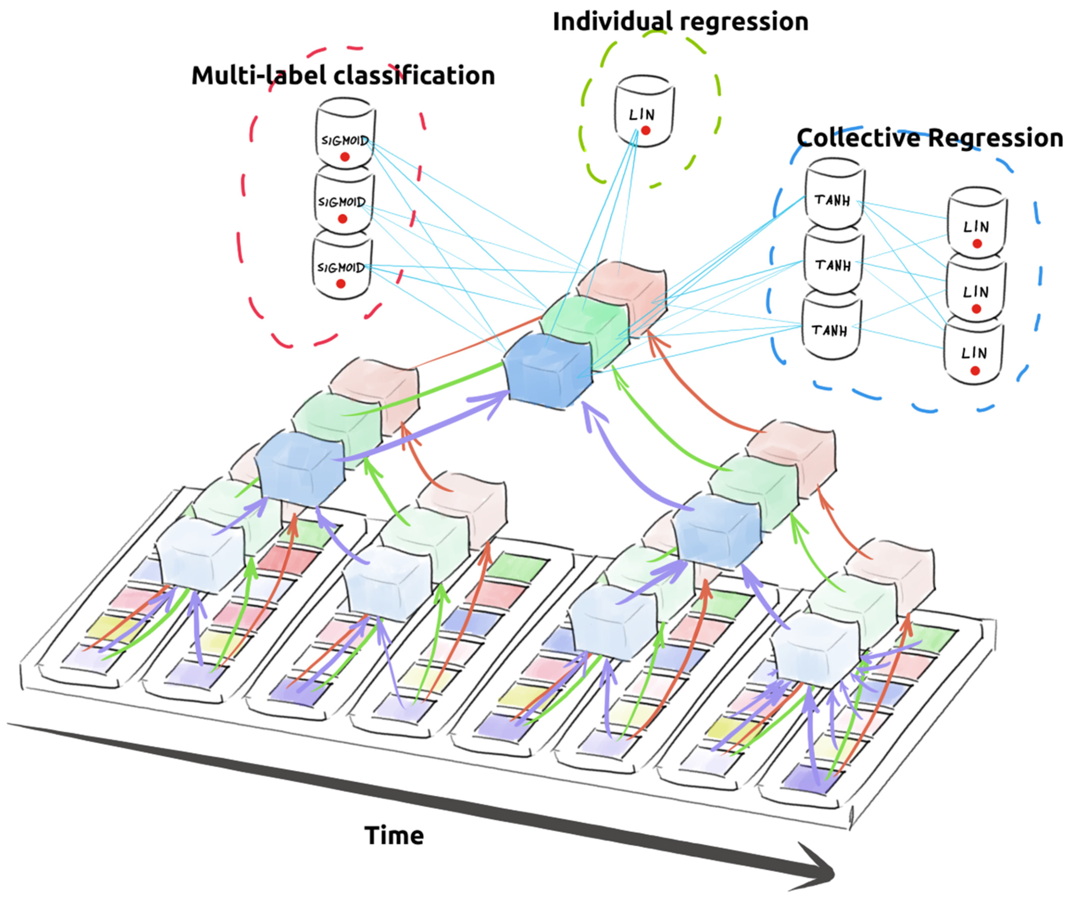
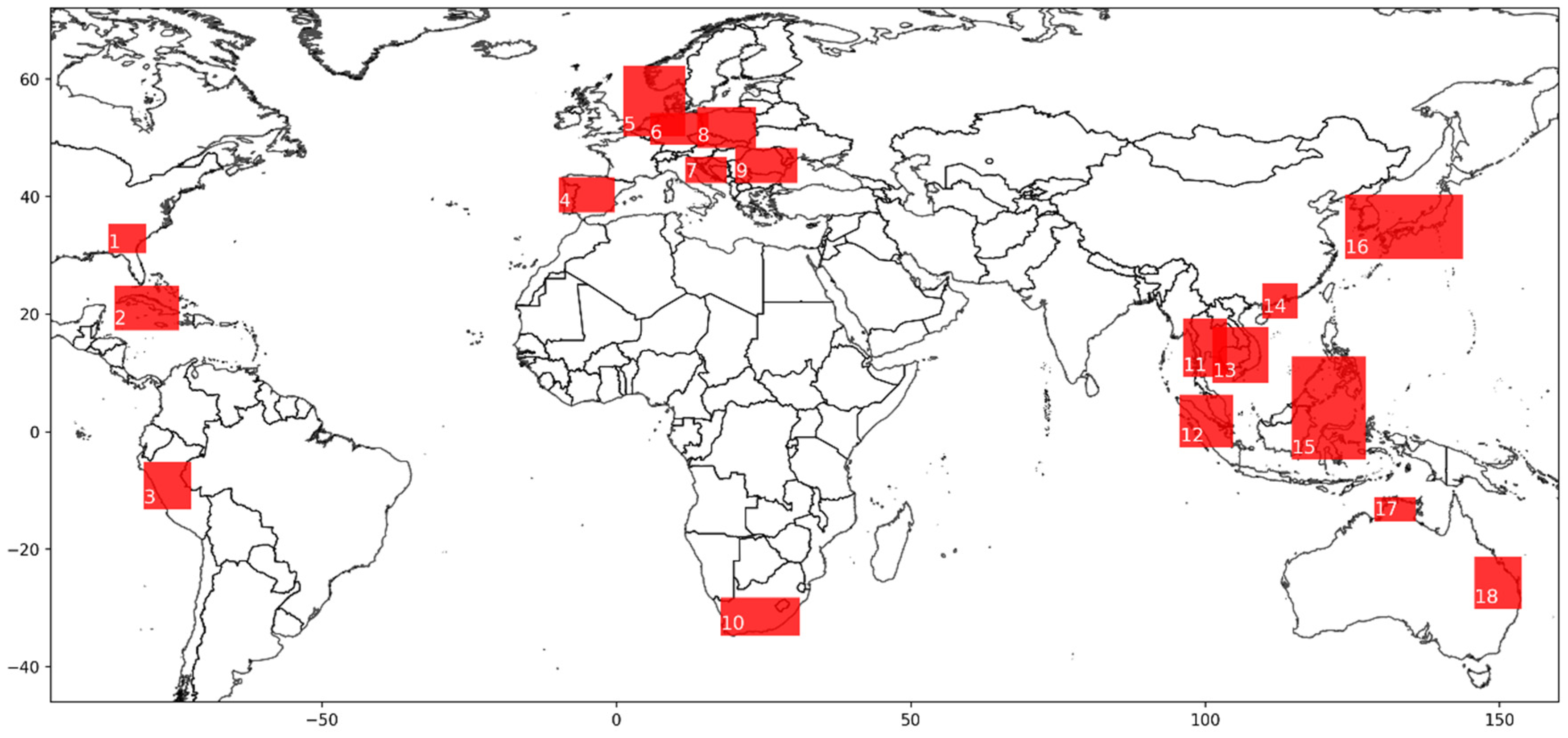
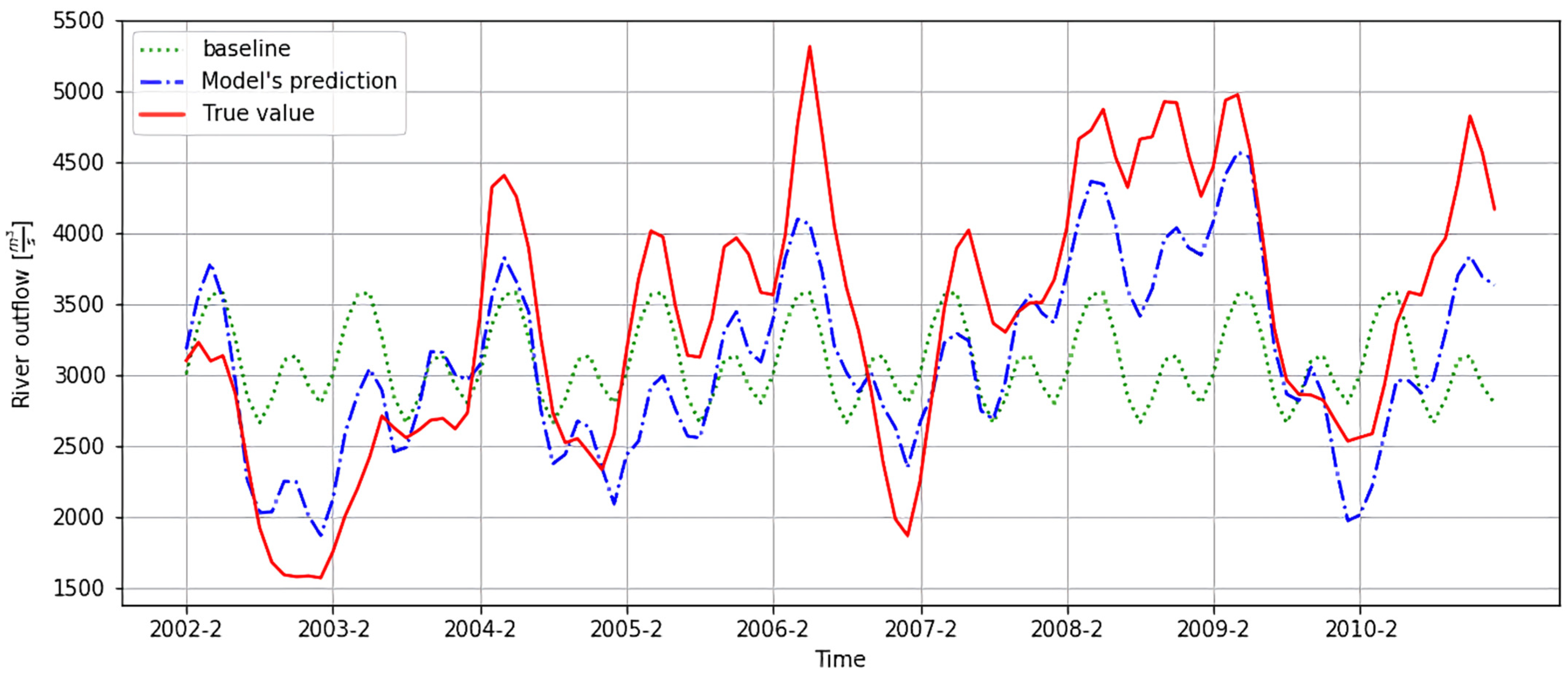
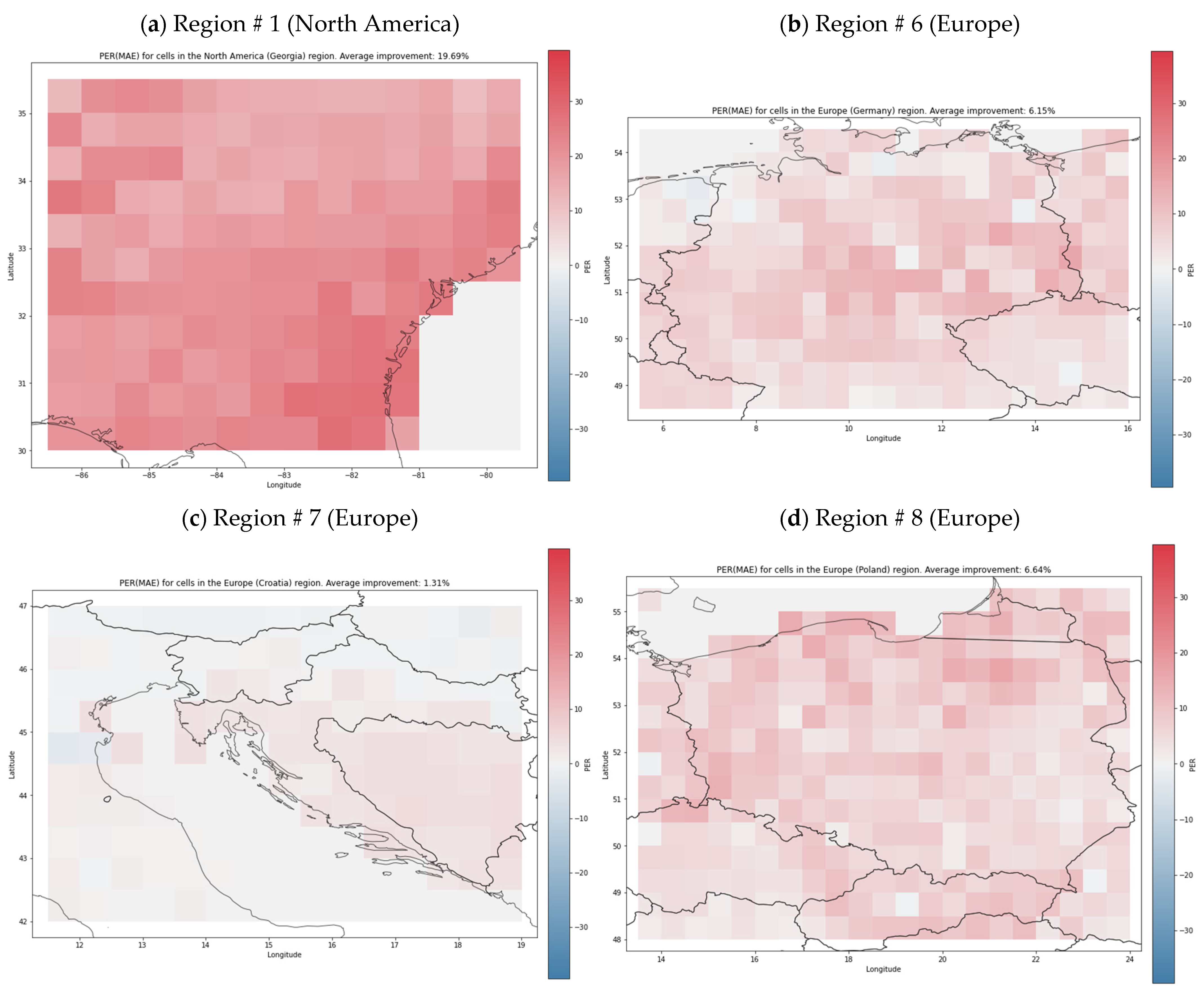
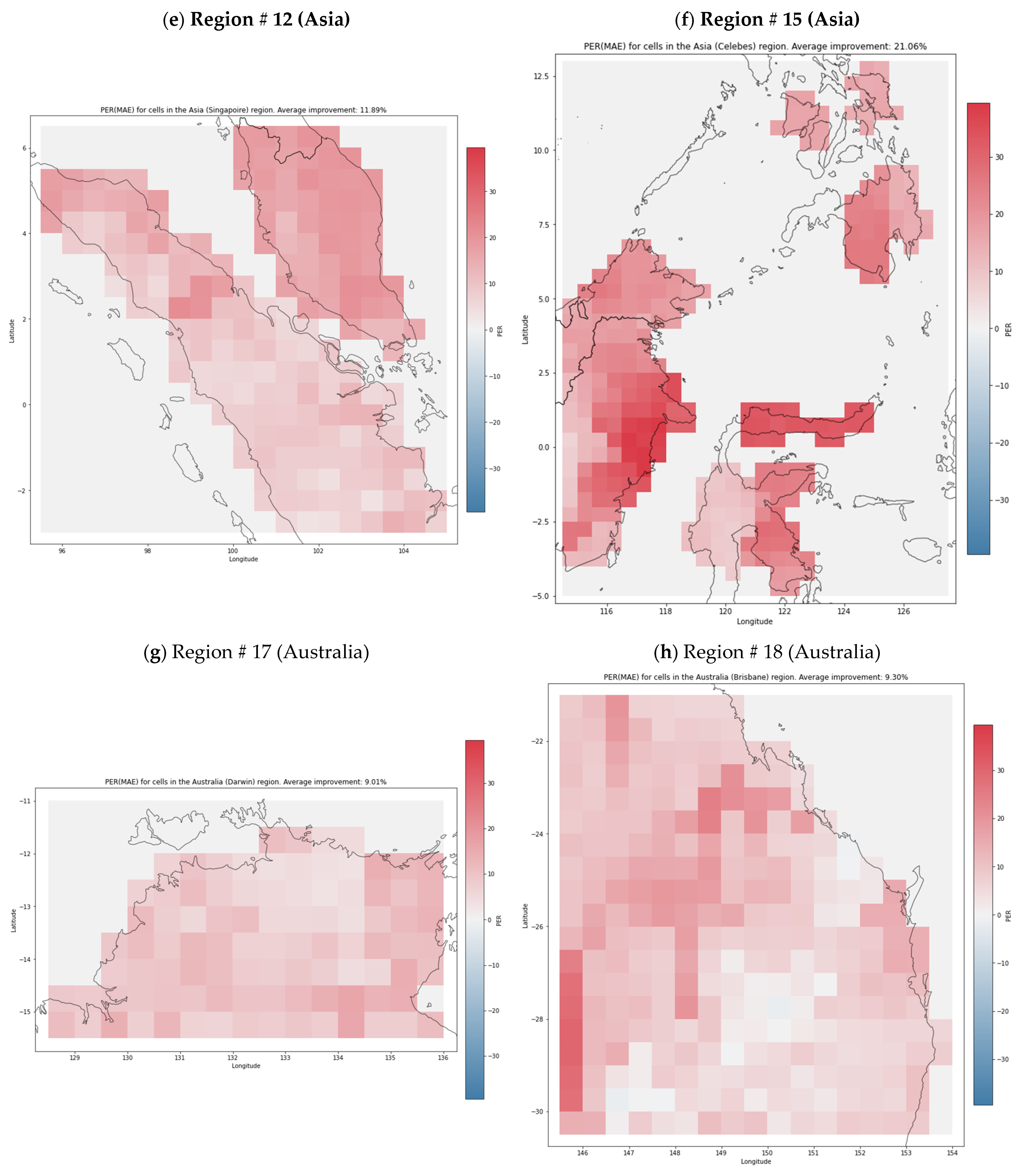
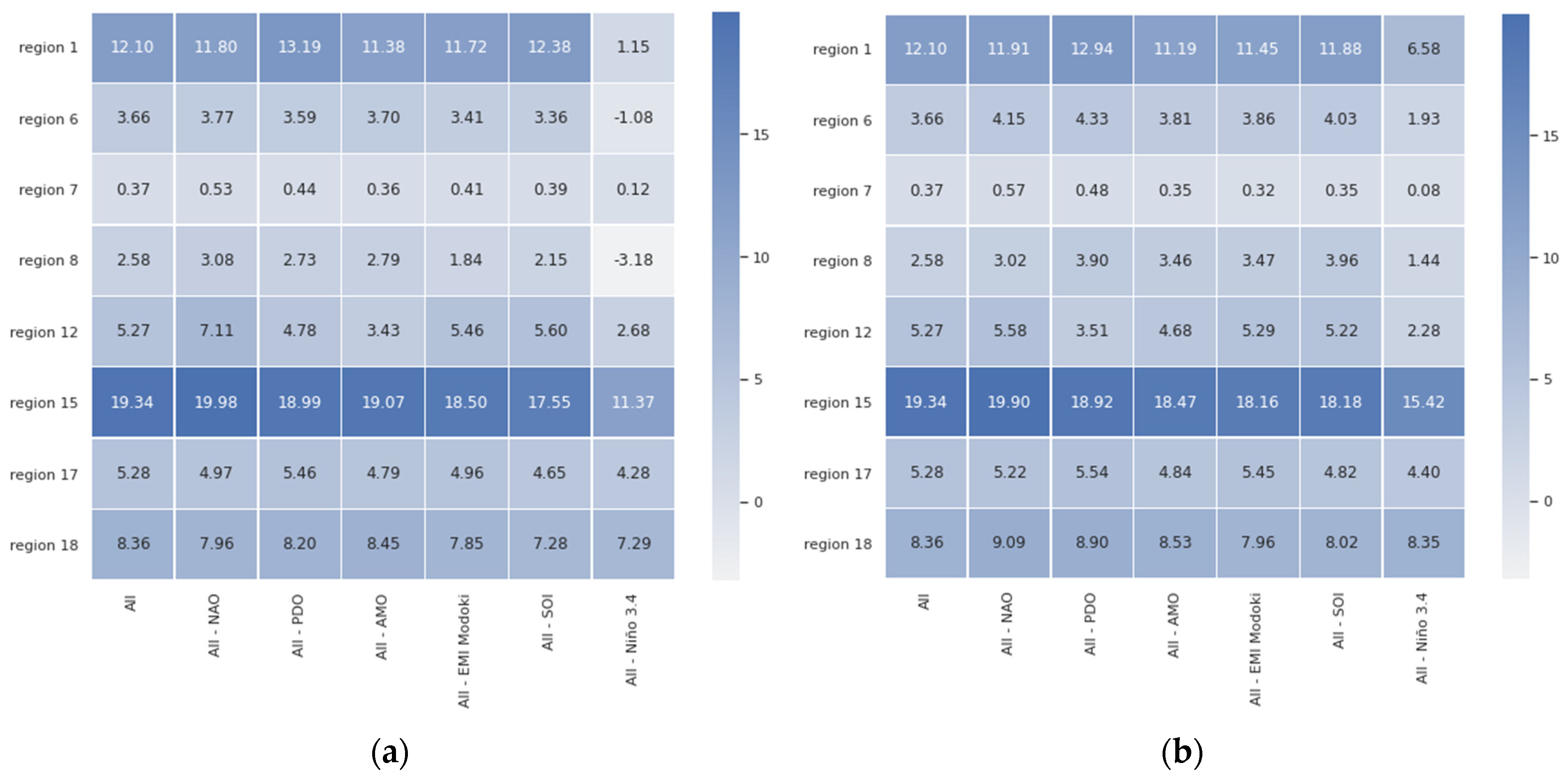
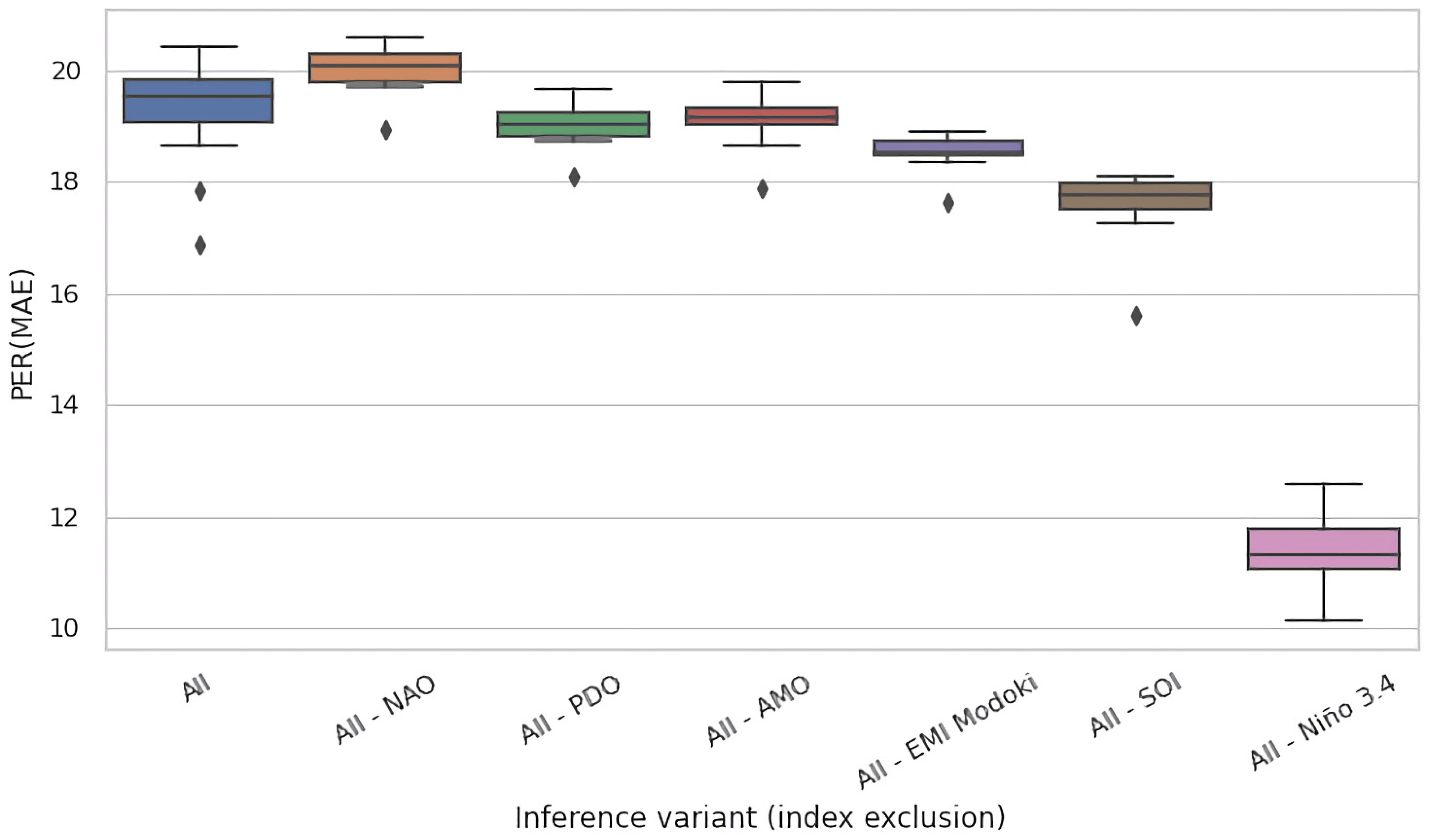
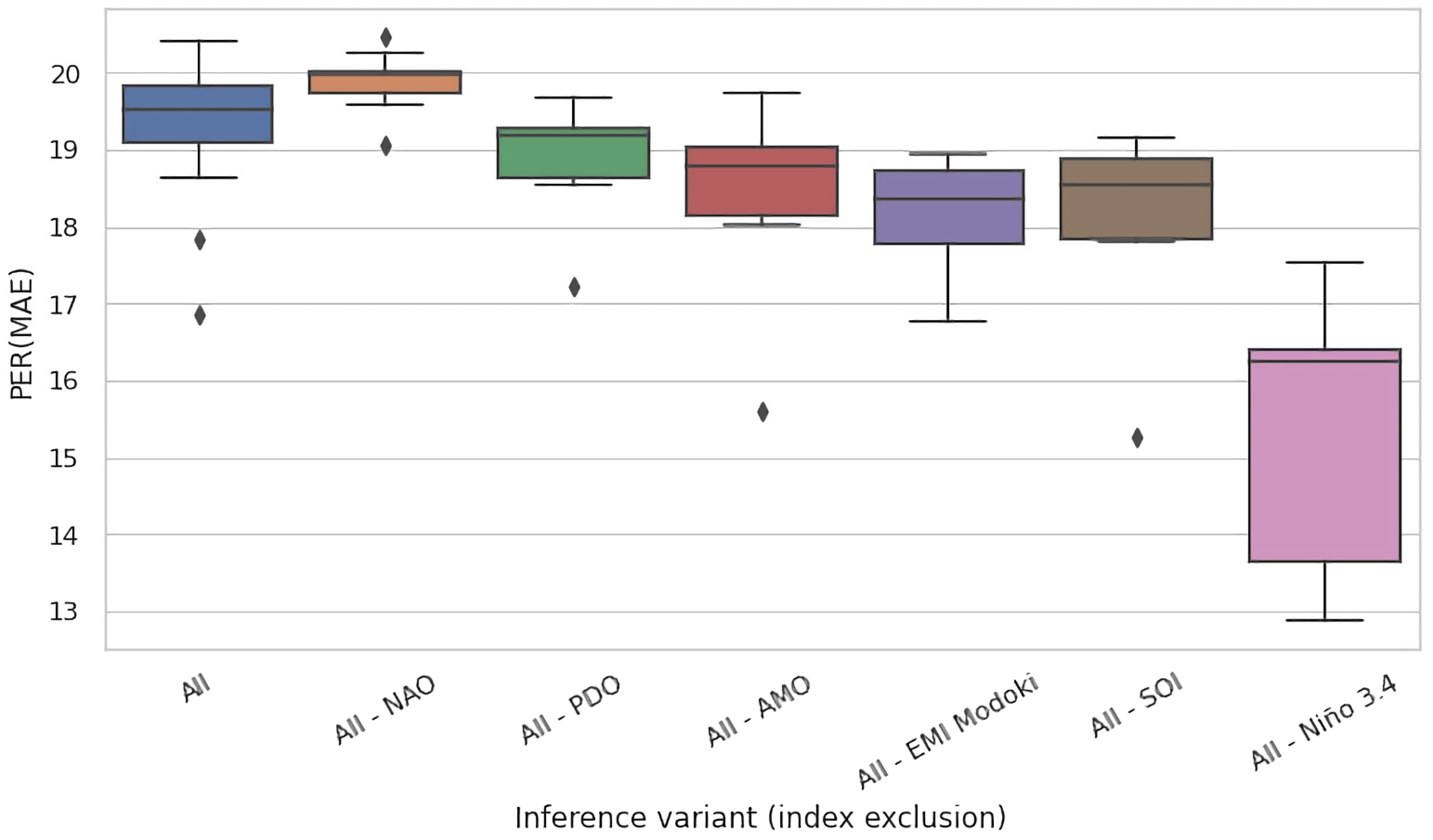
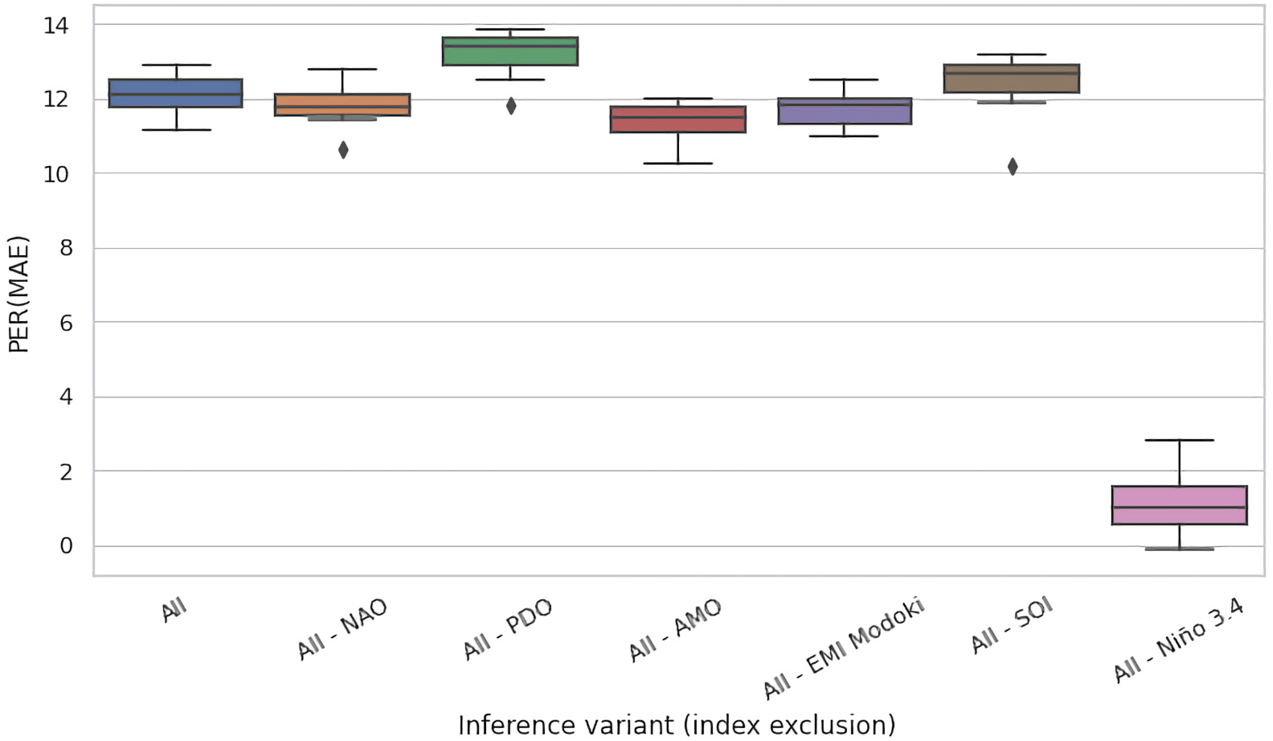
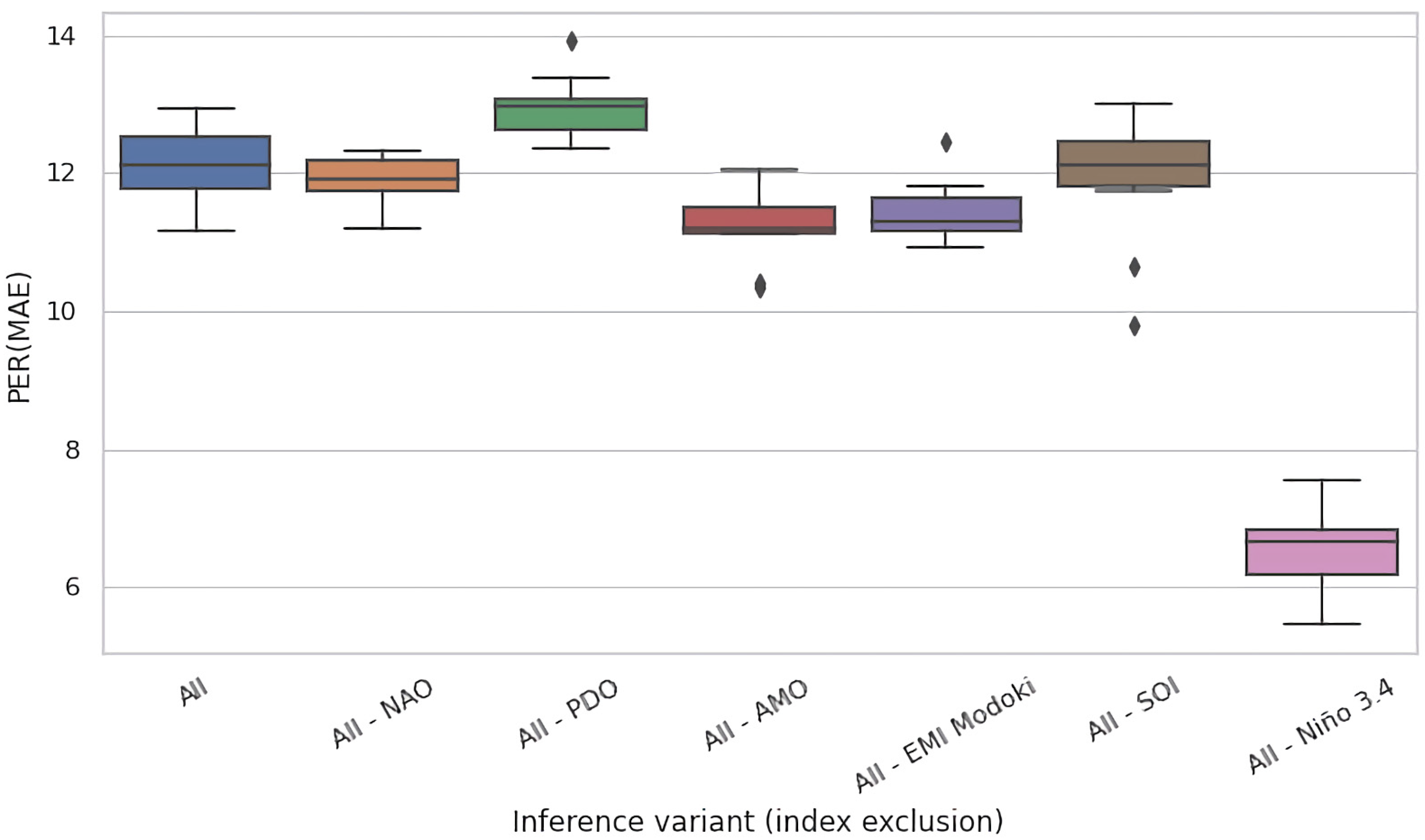
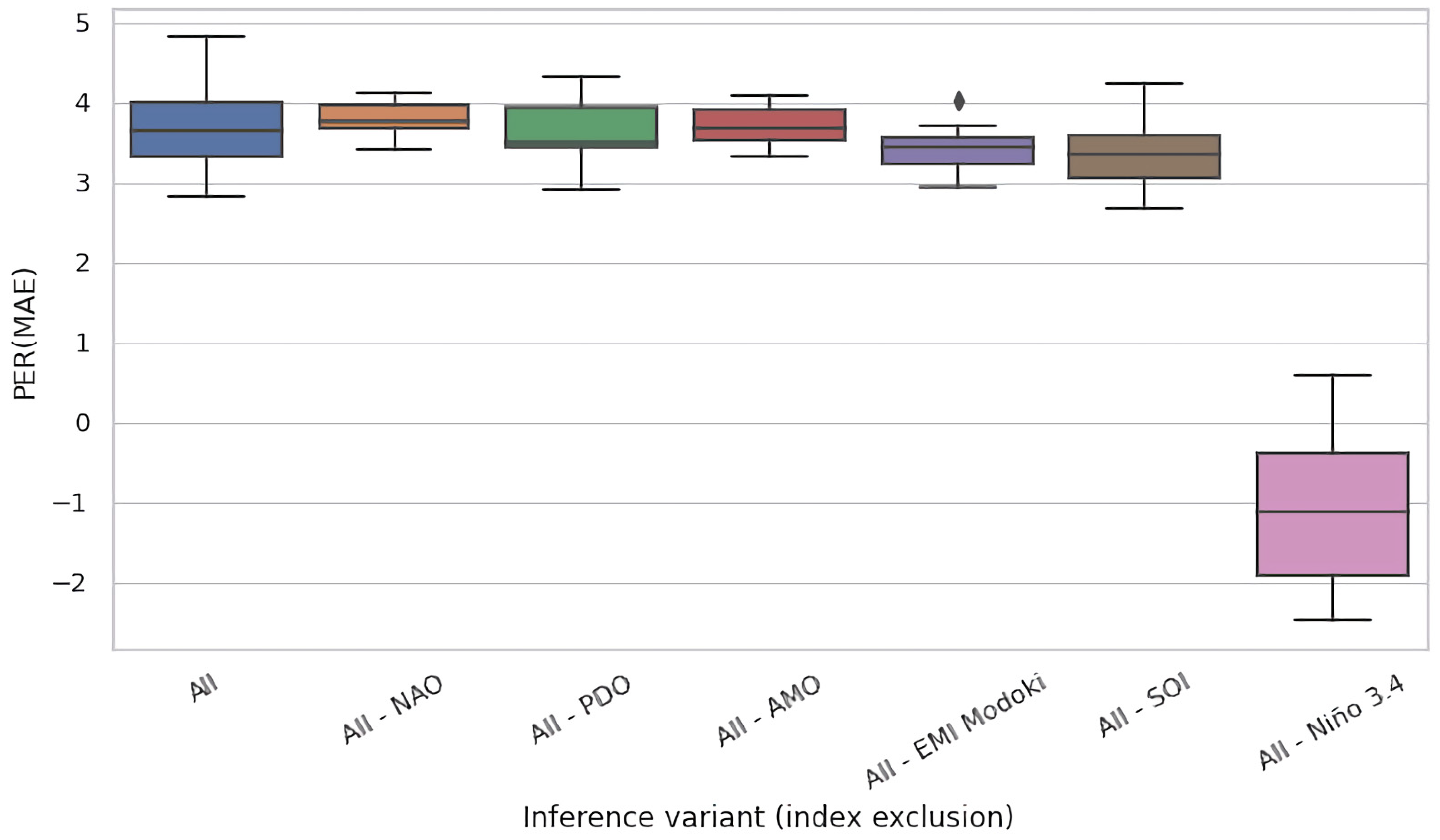
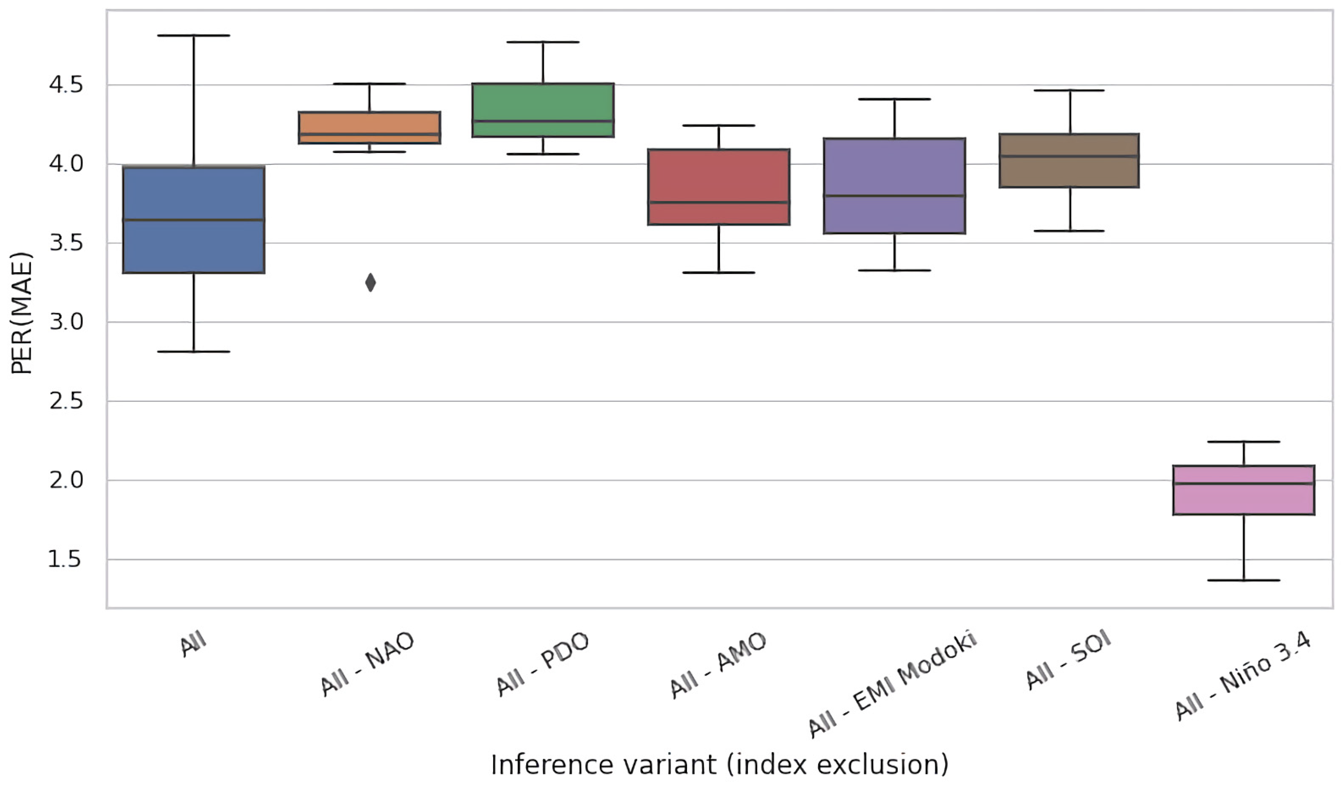
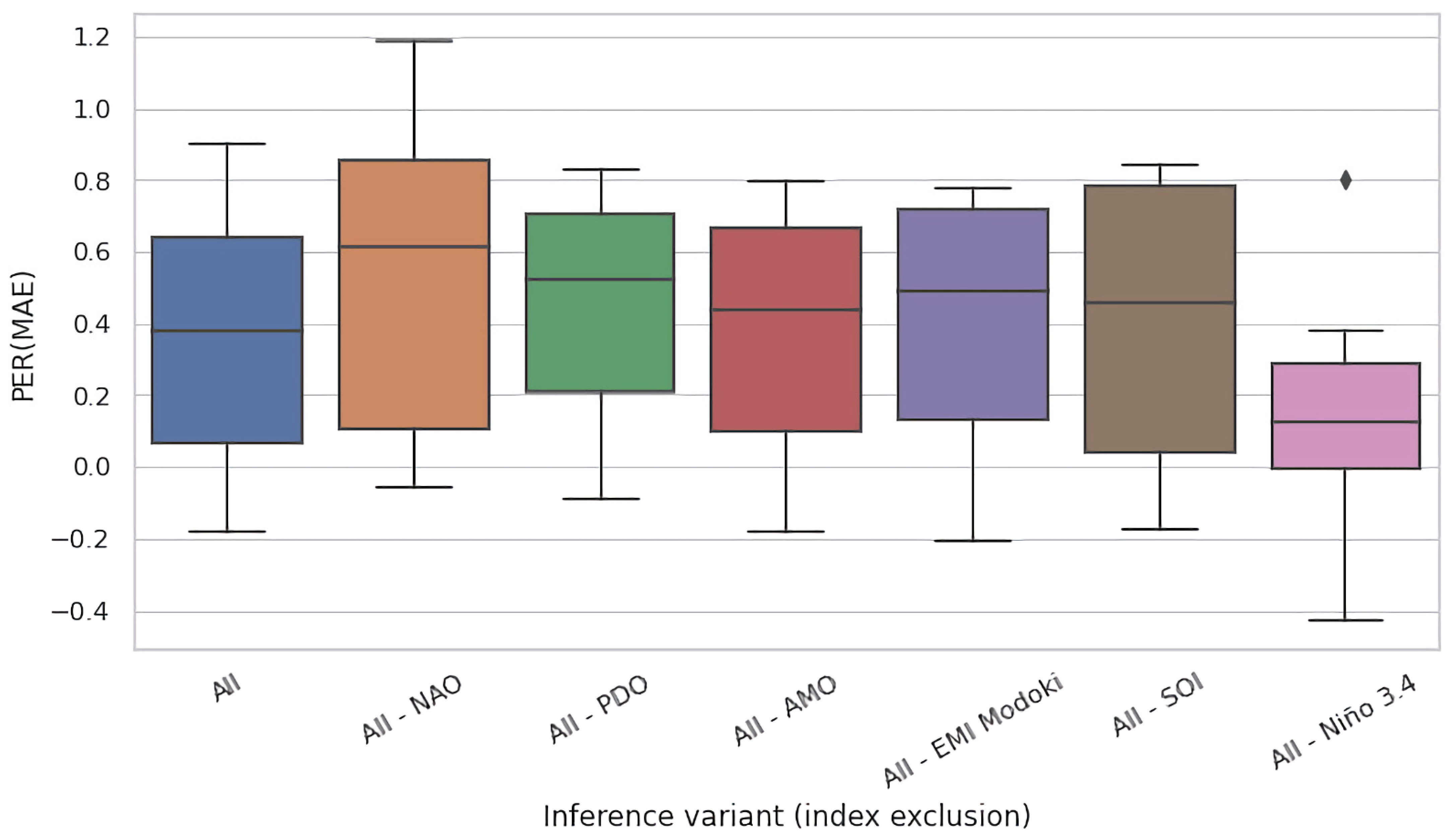
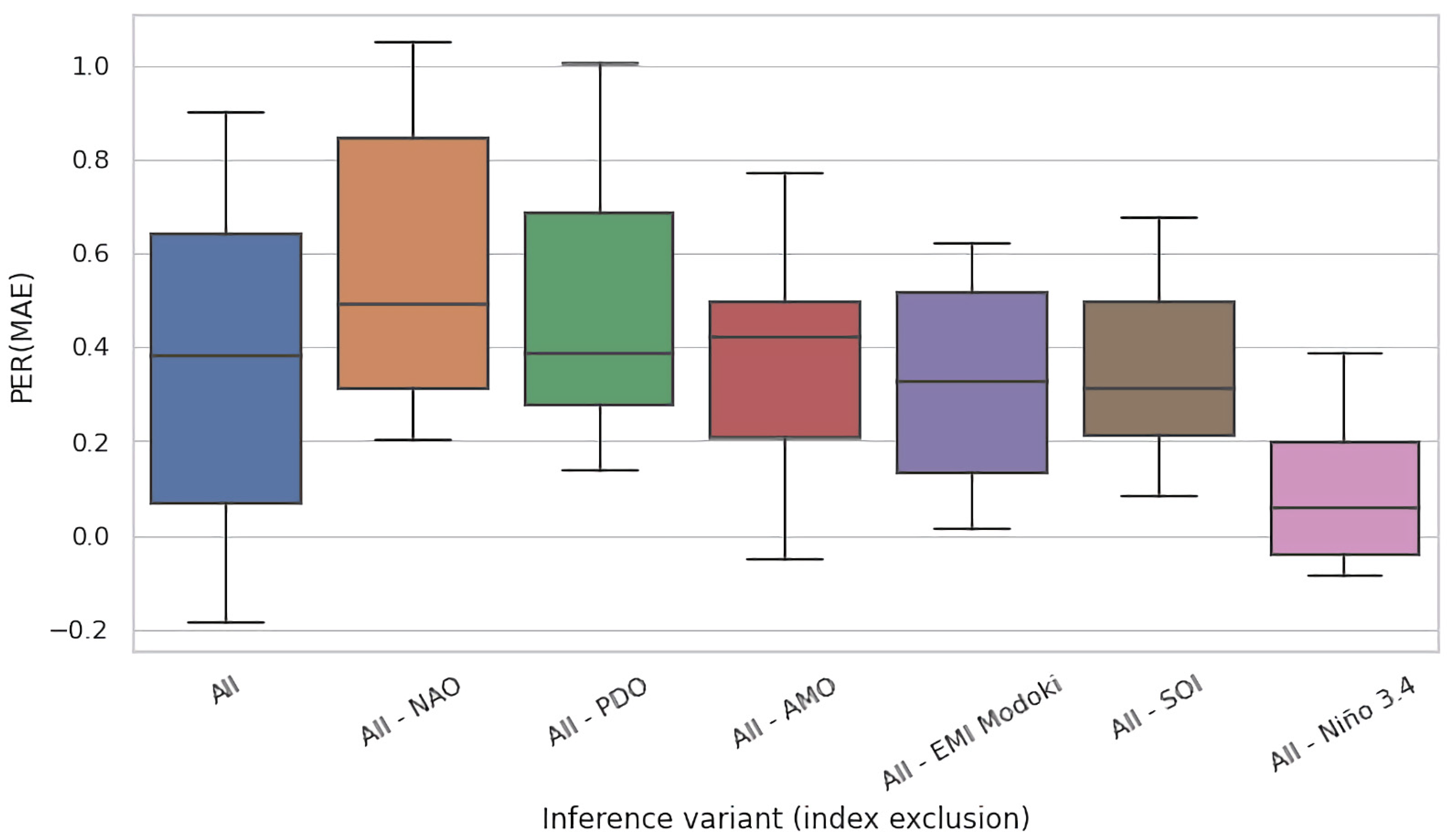
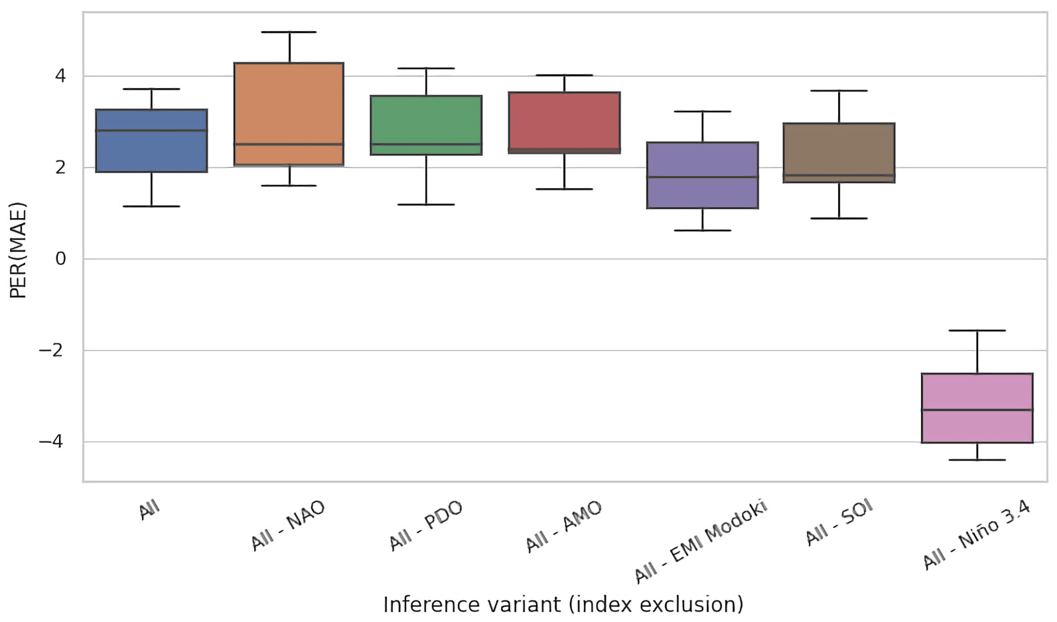
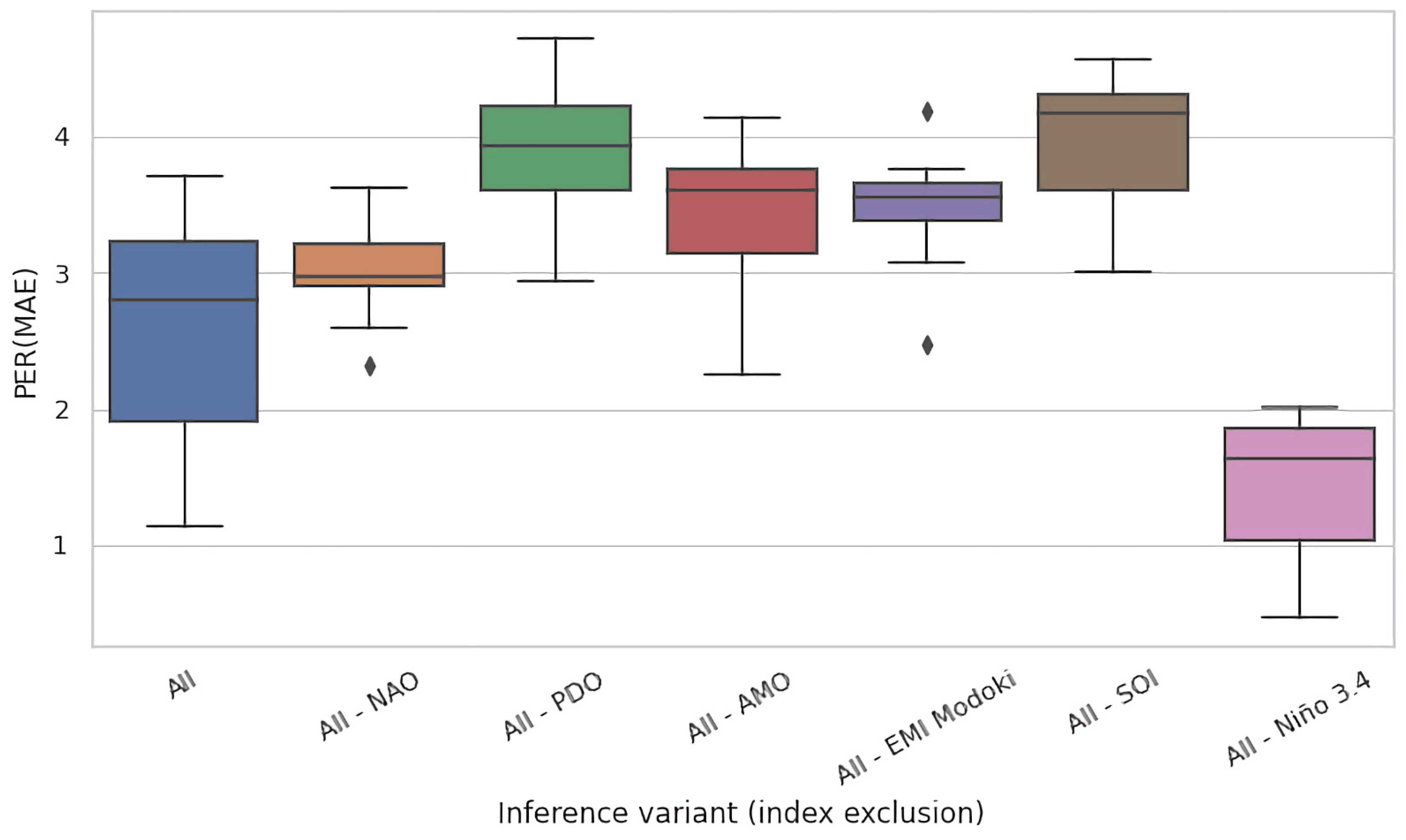
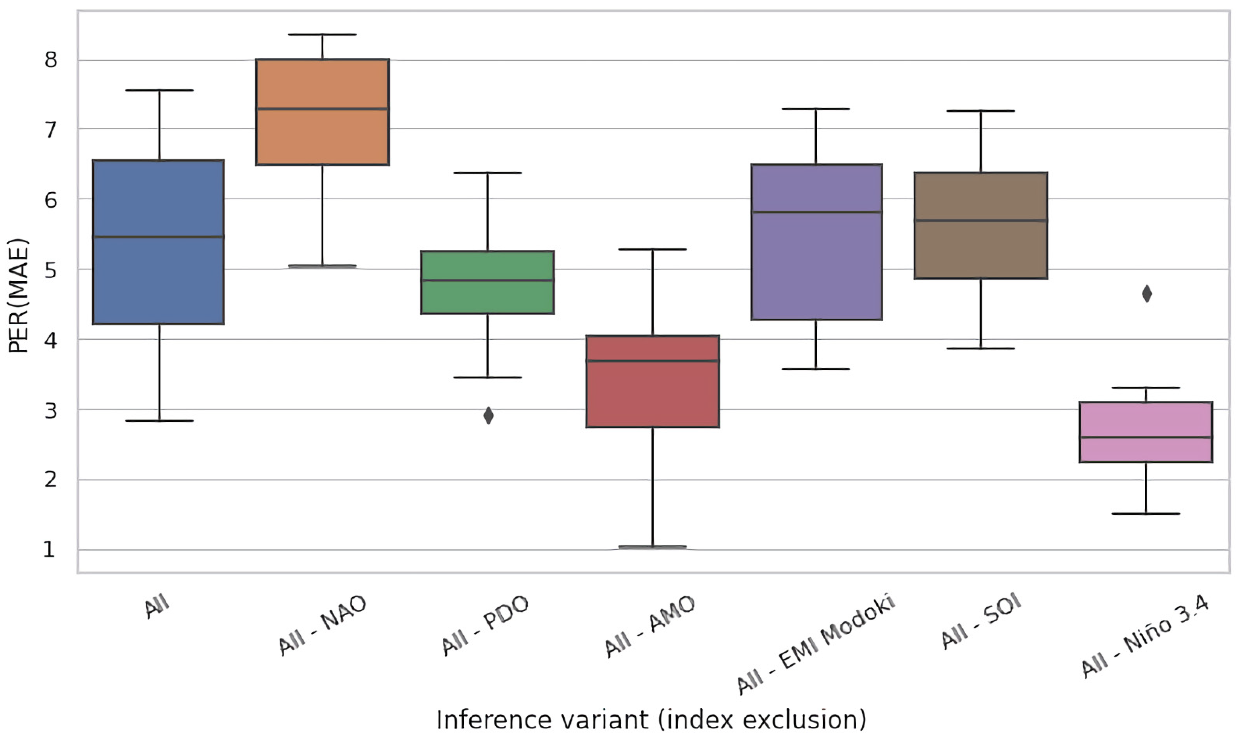
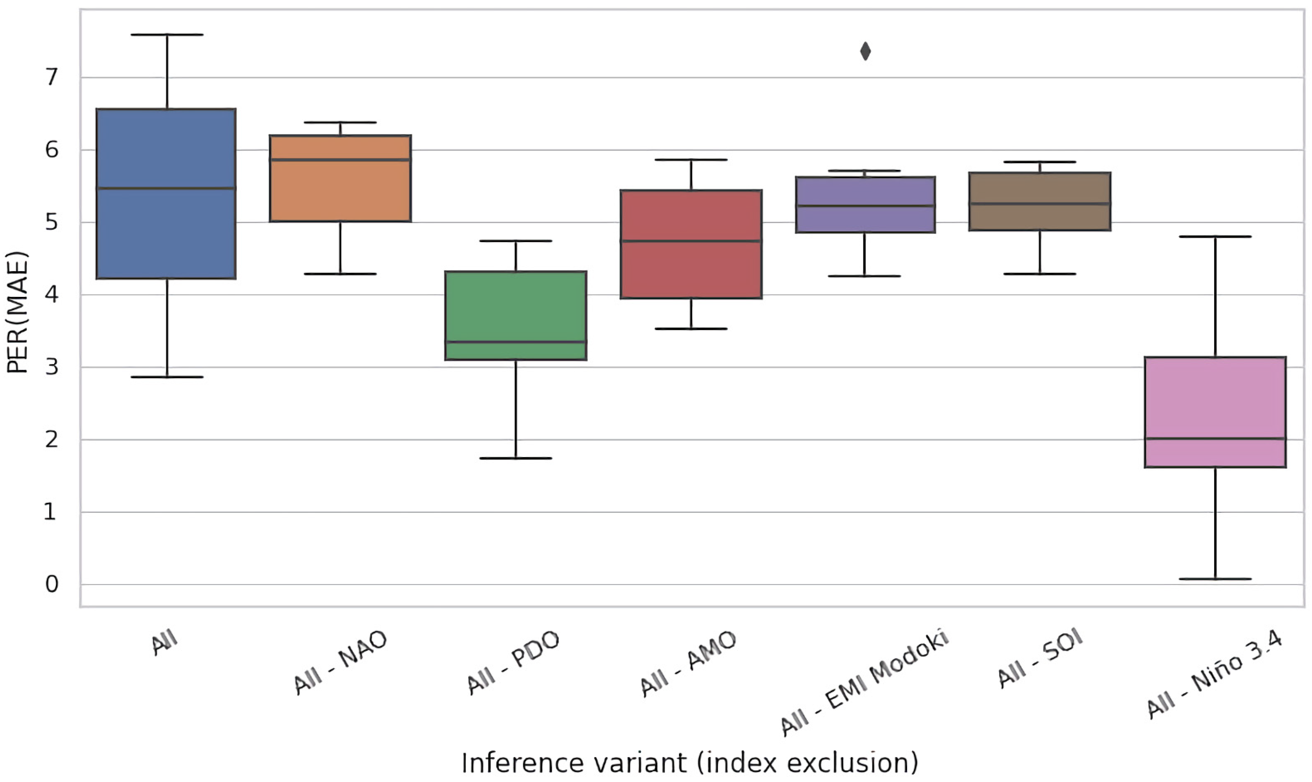
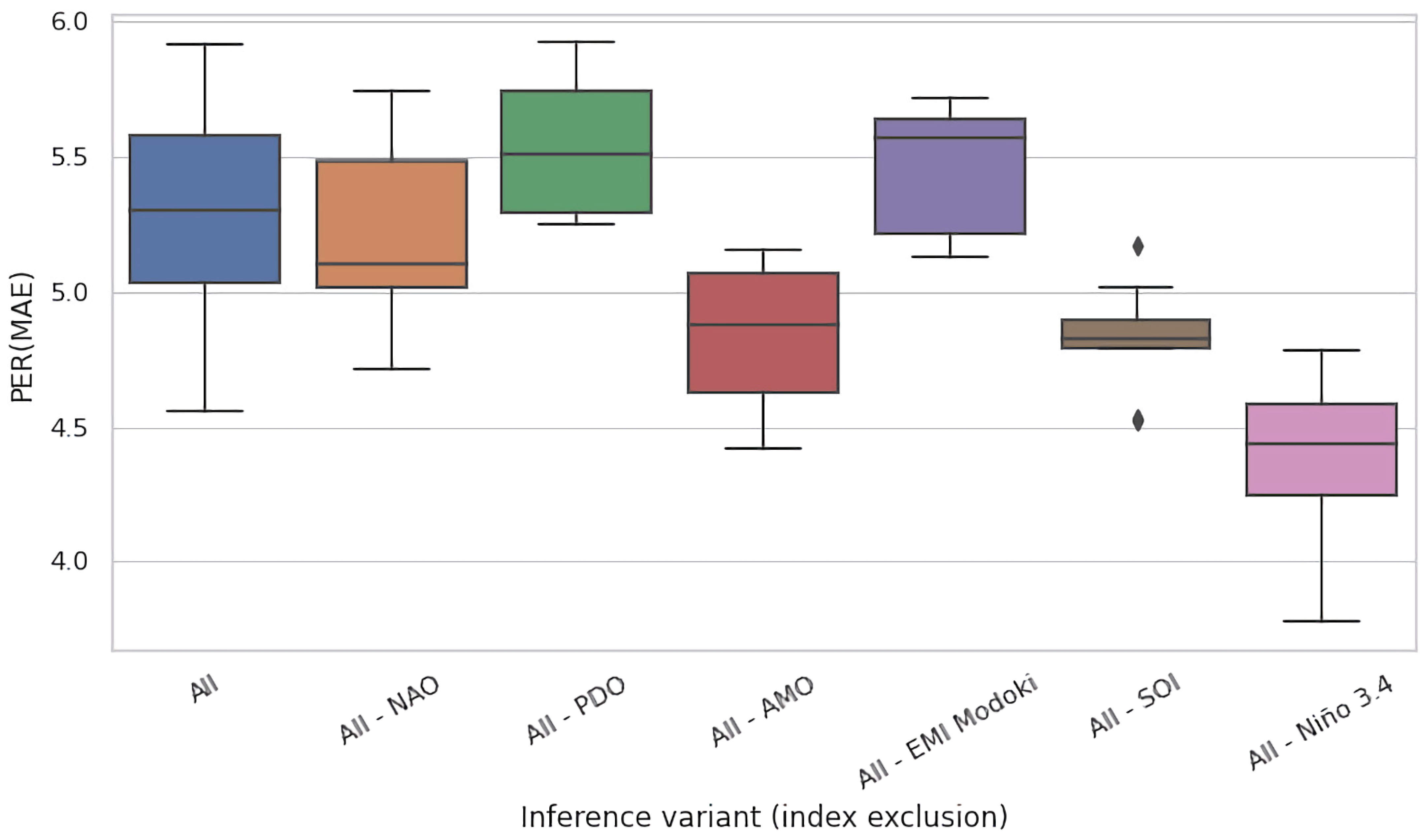
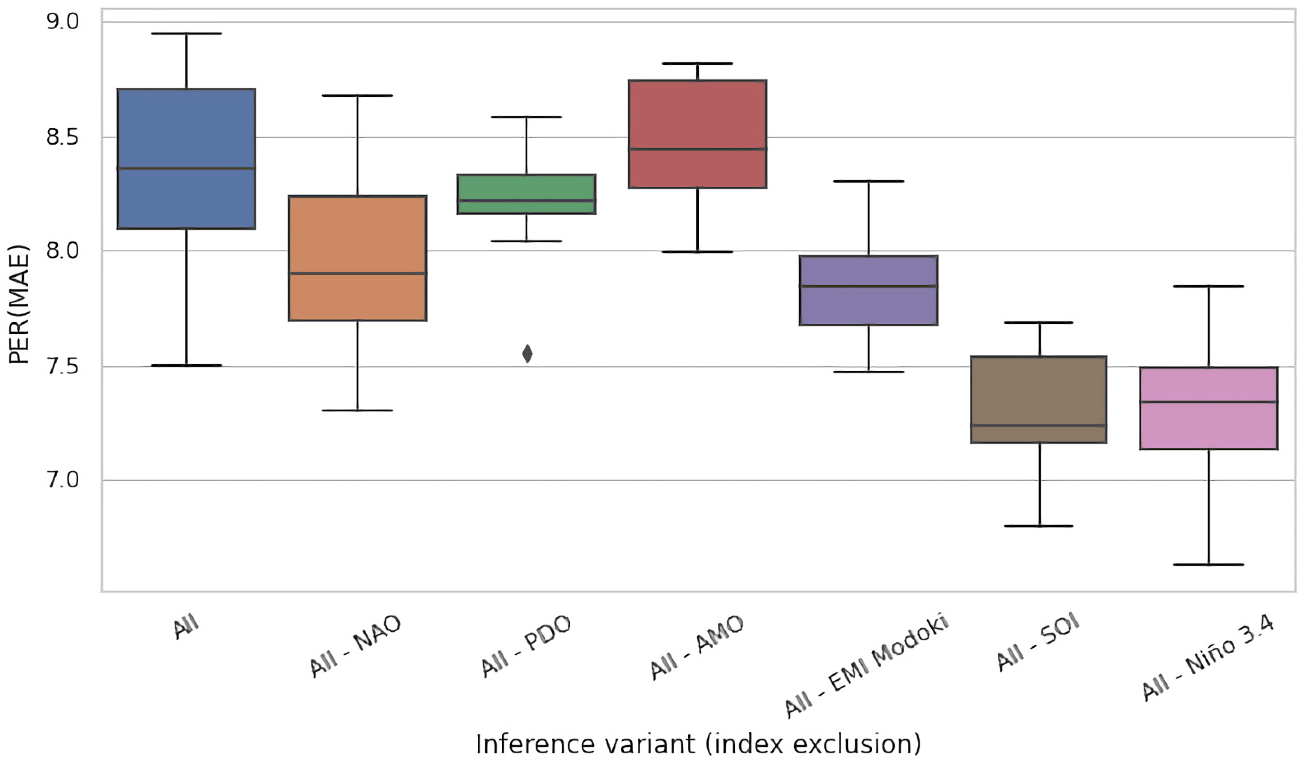
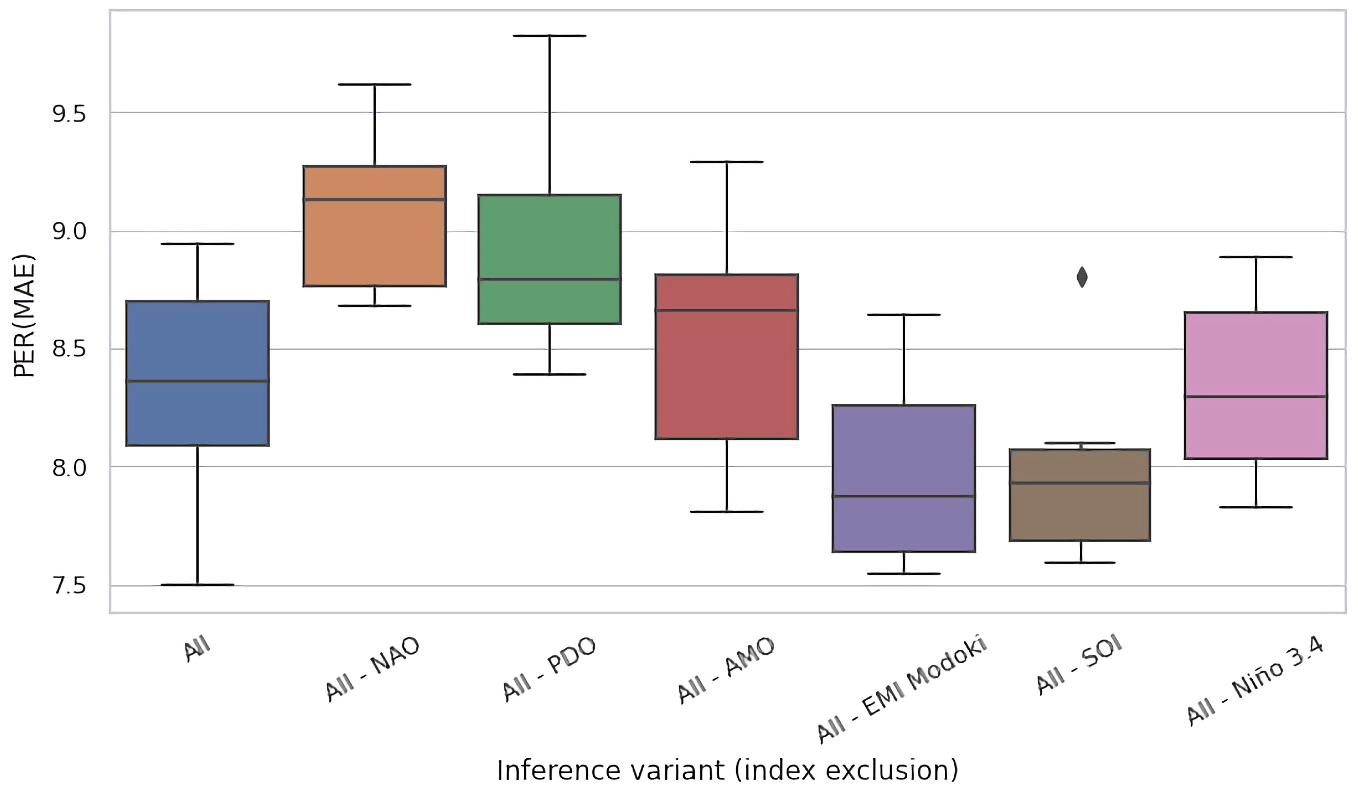
Table 1.
Sources of climate variability indices (all entries accessed on 22 April 2021).
Table 2.
Specification of 18 study areas: location, number of available cells, and values of 3 considered quality metrics. The numbers represent per-region averages (averages over all cells in a region) averaged over 5 models obtained in 5 independent runs of a given configuration. Standard deviations calculated over runs.
| Multivariate | Univariate | ||||||||
|---|---|---|---|---|---|---|---|---|---|
| ID | Lat. | Long. | # of Alid Cells | PER(MAE) | PER(DTW) | PER(TEEE) | PER(MAE) | PER(DTW) | PER(TEEE) |
| 1 | 30° N–36° N | 86.5° W–79° W | 140 | 20.37 ± 1.24 | 14.28 ± 0.67 | 31.08 ± 1.36 | 18.28 ± 0.10 | 12.19 ± 0.13 | 27.65 ± 0.22 |
| 2 | 17° N–25.5° N | 85.5° W–73.5° W | 49 | 3.36 ± 0.21 | 3.62 ± 0.16 | 1.54 ± 0.33 | 2.23 ± 0.30 | 3.05 ± 0.28 | 4.80 ± 0.51 |
| 3 | 13.5° S–4.5° S | 80.5° W–71.5° W | 233 | −0.02 ± 1.24 | −2.63 ± 1.15 | 4.36 ± 0.89 | 0.06 ± 0.16 | −2.47 ± 0.19 | 3.41 ± 0.16 |
| 4 | 37° N–44° N | 10° W–0.5° E | 235 | 3.39 ± 0.32 | 1.94 ± 0.29 | 2.66 ± 1.72 | 2.45 ± 0.12 | 1.52 ± 0.02 | 4.26 ± 0.57 |
| 5 | 50° N–63° N | 1° E–12.5° E | 287 | 1.67 ± 0.74 | 0.95 ± 0.52 | – | 3.30 ± 0.06 | 2.13 ± 0.05 | – |
| 6 | 48.5° N–55° N | 5.5° E–16.5° E | 237 | 4.8 ± 0.43 | 2.72 ± 0.35 | 4.63 ± 0.76 | 6.83 ± 0.05 | 4.01 ± 0.05 | 6.15 ± 0.55 |
| 7 | 42° N–47.5° N | 11.5° E–19.5° E | 118 | 0.85 ± 0.48 | 0.97 ± 0.26 | 0.8 ± 0.58 | 0.56 ± 0.08 | 1.07 ± 0.24 | 0.85 ± 0.23 |
| 8 | 48° N–56° N | 13.5° E–24.5° E | 290 | 7.14 ± 0.94 | 5.09 ± 0.56 | 7.17 ± 1.05 | 9.08 ± 0.09 | 6.45 ± 0.04 | 10.84 ± 0.33 |
| 9 | 42° N–49° N | 20° E–31.5° E | 256 | 3.04 ± 0.57 | 1.98 ± 0.38 | 6.05 ± 0.89 | 2.52 ± 0.08 | 1.53 ± 0.17 | 7.20 ± 0.77 |
| 10 | 27.5° S–35° S | 17.5° E–32° E | 313 | 5.75 ± 0.27 | 2.71 ± 0.19 | 3.28 ± 0.4 | 5.54 ± 0.12 | 2.66 ± 0.11 | 2.29 ± 0.34 |
| 11 | 9° N–20° N | 96° E–104.5° E | 224 | −1.3 ± 0.26 | −0.73 ± 0.14 | −0.21 ± 0.31 | −2.62 ± 0.17 | −2.34 ± 0.10 | −0.88 ± 0.44 |
| 12 | 3° S–7° N | 95.5° E–103.5° E | 187 | 11.06 ± 0.73 | 5.58 ± 0.37 | 10.58 ± 1.31 | 11.30 ± 0.08 | 5.54 ± 0.15 | 9.92 ± 0.56 |
| 13 | 8° N–18.5° N | 101° E–111.5° E | 237 | 0.96 ± 0.38 | 0.86 ± 0.2 | 3.57 ± 0.63 | −1.41 ± 0.13 | −1.38 ± 0.06 | 2.57 ± 0.51 |
| 14 | 19° N–26° N | 109.5° E–116.5° E | 108 | 2.84 ± 0.85 | 0.61 ± 0.6 | −0.78 ± 0.48 | 0.92 ± 0.08 | −0.88 ± 0.12 | −1.16 ± 0.69 |
| 15 | 5° S–13.5° N | 114.5° E–128° E | 273 | 21.27 ± 0.32 | 20.89 ± 0.19 | 17.03 ± 0.49 | 19.30 ± 0.12 | 19.68 ± 0.16 | 14.83 ± 0.61 |
| 16 | 29° N–41° N | 123.5° E–144.5° E | 241 | −0.15 ± 0.46 | 0.71 ± 0.34 | 1.58 ± 1.48 | −1.17 ± 0.08 | 0.55 ± 0.05 | 0.68 ± 0.43 |
| 17 | 10.5° S–15.5° S | 128.5° E–136.5° E | 94 | 8.76 ± 0.81 | 4.29 ± 0.82 | 12.3 ± 1.25 | 5.92 ± 0.21 | 2.70 ± 0.26 | 9.00 ± 0.60 |
| 18 | 21° S–30.5° S | 145.5° E–154.5° E | 263 | 9.18 ± 1.41 | 11.55 ± 2.11 | 9.62 ± 3.85 | 8.46 ± 0.14 | 11.71 ± 0.20 | 10.01 ± 0.19 |
| Mean | 210.3 | 5.72 | 4.18 | 6.78 | 5.09 | 3.76 | 2.06 | ||
Publisher’s Note: MDPI stays neutral with regard to jurisdictional claims in published maps and institutional affiliations. |
© 2021 by the authors. Licensee MDPI, Basel, Switzerland. This article is an open access article distributed under the terms and conditions of the Creative Commons Attribution (CC BY) license (https://creativecommons.org/licenses/by/4.0/).
Share and Cite
MDPI and ACS Style
Norel, M.; Krawiec, K.; Kundzewicz, Z.W. Machine Learning Modeling of Climate Variability Impact on River Runoff. Water 2021, 13, 1177. https://doi.org/10.3390/w13091177
AMA Style
Norel M, Krawiec K, Kundzewicz ZW. Machine Learning Modeling of Climate Variability Impact on River Runoff. Water. 2021; 13(9):1177. https://doi.org/10.3390/w13091177
Chicago/Turabian StyleNorel, Mateusz, Krzysztof Krawiec, and Zbigniew W. Kundzewicz. 2021. "Machine Learning Modeling of Climate Variability Impact on River Runoff" Water 13, no. 9: 1177. https://doi.org/10.3390/w13091177
Note that from the first issue of 2016, this journal uses article numbers instead of page numbers. See further details here.