Inversion of Chlorophyll-a Concentration in Donghu Lake Based on Machine Learning Algorithm

Abstract

Machine learning algorithm, as an important method for numerical modeling, has been widely used for chlorophyll-a concentration inversion modeling. In this work, a variety of models were built by applying five kinds of datasets and adopting back propagation neural network (BPNN), extreme learning machine (ELM), support vector machine (SVM). The results revealed that modeling with multi-factor datasets has the possibility to improve the accuracy of inversion model, and seven band combinations are better than seven single bands when modeling, Besides, SVM is more suitable than BPNN and ELM for chlorophyll-a concentration inversion modeling of Donghu Lake. The SVM model based on seven three-band combination dataset (SVM3) is the best inversion one among all multi-factor models that the mean relative error (MRE), mean absolute error (MAE), root mean square error (RMSE) of the SVM model based on single-factor dataset (SF-SVM) are 30.82%, 9.44 μg/L and 12.66 μg/L, respectively. SF-SVM performs best in single-factor models, MRE, MAE, RMSE of SF-SVM are 28.63%, 13.69 μg/L and 16.49 μg/L, respectively. In addition, the simulation effect of SVM3 is better than that of SF-SVM. On the whole, an effective model for retrieving chlorophyll-a concentration has been built based on machine learning algorithm, and our work provides a reliable basis and promotion for exploring accurate and applicable chlorophyll-a inversion model.

1. Introduction

Lake eutrophication has become a global common environmental problem [1], which exacerbates the deterioration of the global water environment and the shortage of water resource [2,3]. Chlorophyll-a concentration is an index for estimating primary productivity and biomass in lake ecosystem [4,5], and it is an important indicator of lake eutrophication [6,7]. Therefore, it is of great signification to monitor the concentration of chlorophyll-a in lake water.

The traditional method of monitoring chlorophyll-a concentration is based on a suite of laboratory and situ measures [8], which is time-consuming, costly and regional limited [9]. With the mature development of remote sensing technology and deepening research on spectral characteristics of water quality parameters, remote sensing inversion has become an economical and effective method for real-time and continuous monitoring of chlorophyll-a concentration in lakes [10,11,12]. Research shows that Chlorophyll-a mainly absorbs red light and blue violet light, the maximum absorption wavelength ranges from 420 nm to 663 nm, and it has a strong reflection of green light [13,14]. Because chlorophyll-a possesses this unique optical property, the inversion model can be built by analysing the statistical relationship between the concentration of chlorophyll-a and the characteristic bands of remote sensing, and then the chlorophyll-a concentration of the whole water body is calculated [15].

When choosing the independent variable to build a chlorophyll-a inversion model, the multi-band combination most relative with chlorophyll-a is more popularly [16,17,18]. However, this operation for modeling does not use the remaining bands, and their influence on chlorophyll-a concentration is ignored. At the same time, the combined effect of multiple factors has not been studied. Therefore, in order to improve the accuracy of inversion, it is necessary to consider all the bands related to chlorophyll-a and study multiple factors modeling.

Machine learning algorithm, as a new method for modeling, does not rely on the fixed model framework, it can constantly learn the feedback error in the process of model correction and improve the complex relationship between independent variables and dependent variables [19]. It is an effective method to solve the nonlinear regression problem, and provides a new method for remote sensing inversion of chlorophyll-a concentration [20,21]. The chlorophyll-a inversion based on machine learning algorithm can be divided into two process: learning the relationship between in situ concentration of chlorophyll-a and band value, then using the functional relationship to calculate chlorophyll-a concentration [22]. This method has the advantage of solving high-dimensional and nonlinear problems [23], as a result, machine learning algorithm model usually shows good inversion effect of chlorophyll-a concentration [24]. For example, artificial neural network, which is used as a common method for lake chlorophyll-a inversion, has been proved to be useful [25,26,27]. The extreme gradient boosting tree (BST), which is employed to develop an algorithm for chlorophyll-a estimation from operational land imager (OLI) in turbid lakes, has also been proved to perform well on a subset of data [28]. A simplified SVM model optimized by genetic algorithm (GA-SVM) was developed for the prediction of monthly concentration of chlorophyll-a in the Miyun Reservoir, and the result showed the model was suitable for the simulation and prediction of chlorophyll-a with better performance in accuracy and efficiency [29]. Therefore, machine learning algorithm can be used as an effective method for chlorophyll-a monitoring [30], and it has been applied to the study of the eutrophication of Donghu Lake. Although many researches have been conducted on remote sensing monitoring of chlorophyll-a concentration in Donghu Lake by using machine learning algorithm [31,32,33], a universal and effective method has not been proposed to realize the long-term monitoring of the chlorophyll-a concentration. The research shows that inversion model has poor universality and is only applicable to a specific area [34,35]. Therefore, it is particularly important to comprehensively compare and fundamentally analyse the impact of various factors on the chlorophyll-a inversion modeling process, and select the best factor to build an effective model for the chlorophyll-a concentration inversion of Donghu Lake.

The main objective in this study is to analyse the impacts of various factors on the process of inversion modeling and build an effective model based on machine learning algorithm for chlorophyll-a concentration inversion of Donghu Lake. The contributions of this work are presented as follows: (a) compare the impacts of single-factor and multi-factor, single-band and multi-band combinations, different machine learning algorithms on model accuracy, respectively; (b) build an effective inversion model for chlorophyll-a concentration in Donghu Lake. Furthermore, our work provided a reliable basis to optimize modeling influence factors based on machine learning algorithm and improve the accuracy of chlorophyll-a concentration inversion model.

2. Materials and Methods

2.1. Study Area

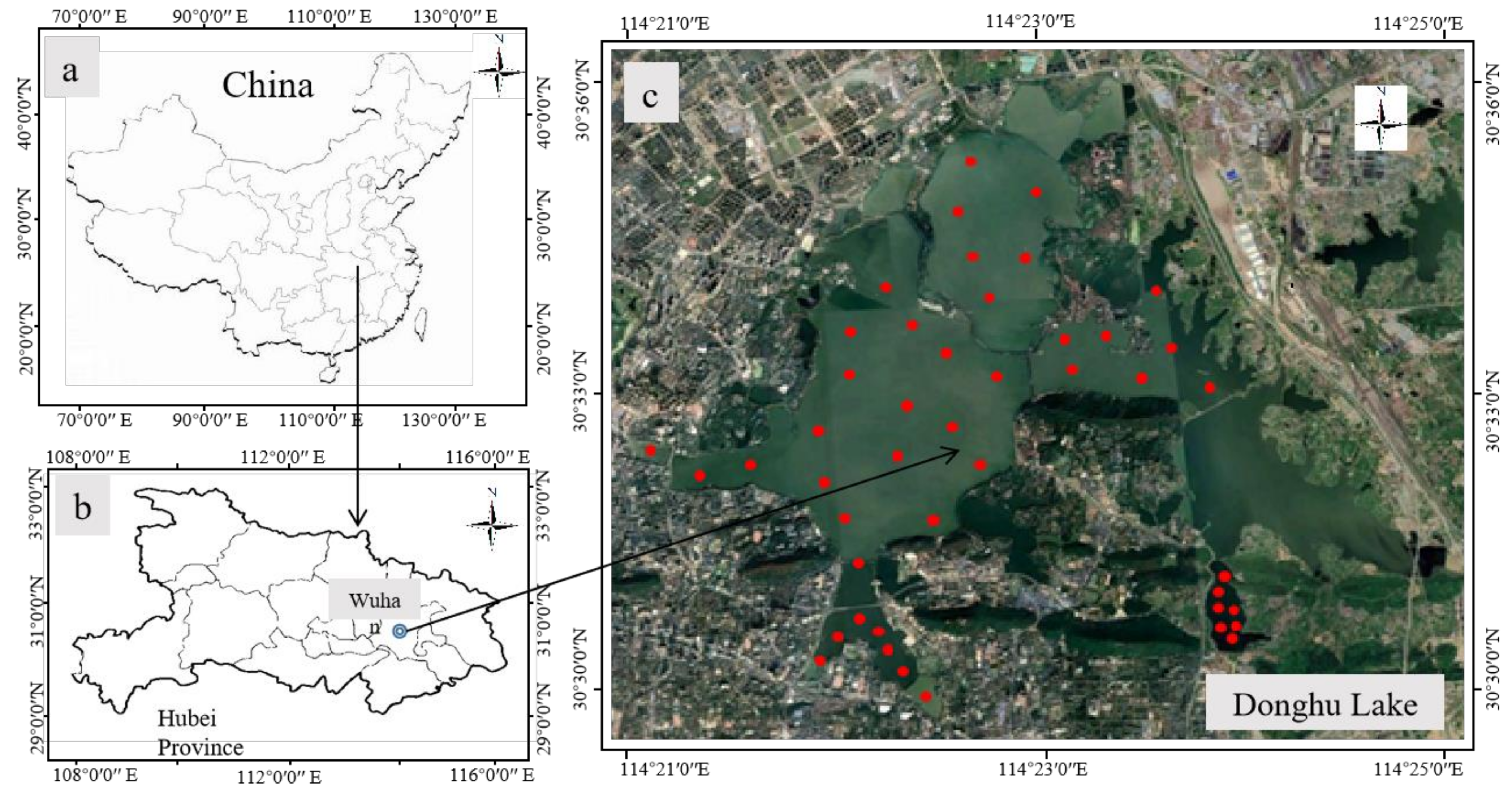
Donghu Lake (30°22′–30°40′ N, 114°09′–114°39′ E) is located in central Wuhan, Hubei Province. It is one of the largest urban lake in China [36], and it is a shallow lake with 32 km² in area, and 2.16 m in average depth and 4.66 m in maximum depth [37]. Donghu Lake is mainly composed of Guozheng Lake, Tangling Lake, Houhu Lake, Tuanhu Lake, Miaohu Lake, Lingjiao Lake, Shuiguo Lake, Yujia Lake and other sub lakes. Donghu Lake provides water for residents, industry and land irrigation, at the same time, it receives all kinds of sewage and waste water discharged from the city [38]. In addition, it has an extensive surface area, a slow water flow and a long water exchange period, and these characteristics make it easy to be polluted by domestic sewage and industrial waste water from the surrounding residents and enterprises. The monitoring data shows that the overall water quality of Donghu Lake has reached the standard of class III, but the water quality category of some sub lakes was at class IV or class V in 2019 (http://www.whdonghu.gov.cn (accessed date on 21 February 2020)). Therefore, the eutrophication of the Donghu Lake is serious. The water environment condition of the Donghu Lake is related to the sustainable development of the city, so it is necessary to monitor the eutrophication of the East Lake comprehensively and systematically. In this study, we try to retrieve the chlorophyll-a concentration of the Donghu Lake from the chlorophyll-a measured data combined with Landsat 8 satellite images based on optimized machine learning inversion model.

To obtain water samples, 45 sampling points were sited with a handheld global positioning system locator recording positions on 17 December 2017 when it was sunny. The sampling points were presented in Figure 1, and the water samples were taken from 0.5 m underwater at every sampling point.

2.2. Material

The water samples were taken back to the laboratory to detect the concentration of chlorophyll-a by Spectrophotometry in HJ 897-2017. Meanwhile, the Lansat8 satellite images on 20 December 2017 were acquired on the website (https://earthexplorer.usgs.gov/ (accessed date on 30 December 2017)), because that day were the closest day with the sampling time which has available images. As we know, the operational land imager (OLI) of Landsat8 consists of nine bands with a spatial resolution of 30 m and a revisit period of 16 days [39]. The image was processed with ENVI5.3 to obtain the spectral reflectance of each sampling point by radiometric calibration, atmospheric correction, image fusion, water extraction, and water colour spectrum extraction. And the database of sampling points location coordinates, band values and chlorophyll-a concentration were established. The band values consisted of Band1 (B1), Band2 (B2), Band3 (B3), Band4 (B4), Band5 (B5), Band6 (B6) and Band7 (B7).

Due to the large differences in the local water quality of Donghu Lake, the chlorophyll-a concentration measured at each sampling point differs greatly, and the chlorophyll-a concentration is between 5.25 μg/L and 157.24 μg/L (in

Table 1. The measured value of chlorophyll-a concentration.

Minimum (μg/L)	Maximum (μg/L)	Average (μg/L)	Standard Deviation(μg/L)
5.25	157.24	46.35	49.02

). From the measured value of chlorophyll-a, there is a big difference among the water quality of the whole Donghu Lake, and some local water has been in a state of eutrophication, and even severe eutrophication.

2.3. Method

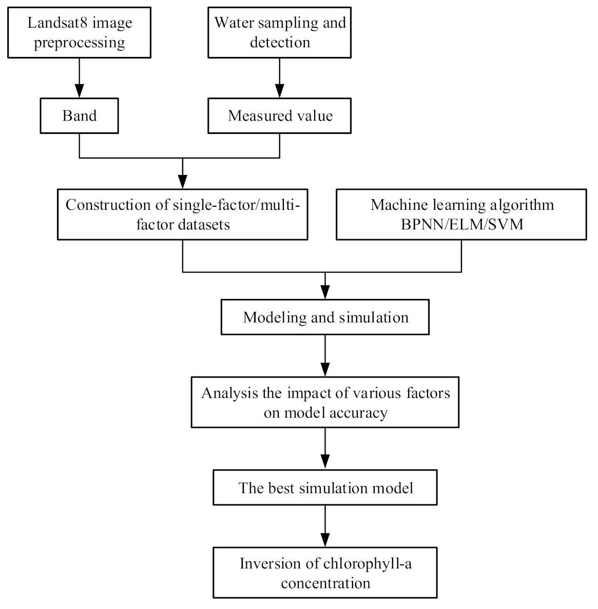
In this study, a series of models are built by combining multiple datasets and BPNN, ELM, SVM. The impact of various factors on model accuracy is analysed to study the best condition for modeling. In addition, the model with best simulation effect is used for the inversion of chlorophyll-a concentration in Donghu Lake. The research flow chart of machine learning algorithm modeling and chlorophyll-a concentration inversion is shown in Figure 2.

2.3.1. Band Selection and Correlation Analysis

There are seven single-band and fifteen kinds of band combinations shown in

Table 2. The single-band and the multi-band combinations.

Band or Combination	Combination Forms
Single-band	Bi, i = 1,2,…,7
Dual-Band Combination	Bi + Bj, Bi − Bj, Bi × Bj, Bi/Bj, i = 1,2,…,7, j = 1,2,…,7, i ≠ j
Three-Band combination	Bi × (Bj + Bk), Bi × (Bj − Bk), Bi/(Bj + Bk), Bi/(Bj − Bk), i = 1,2,…,7, j = 1,2,…,7, k = 1,2,…,7, i ≠ j ≠ k
Four-Band combination	(Bi + Bj) × (Bk + Bl), (Bi + Bj) × (Bk − Bl), (Bi − Bj) × (Bk − Bl), (Bi + Bj)/(Bk + Bl), (Bi + Bj)/(Bk − Bl), (Bi − Bj)/(Bk+Bl), (Bi − Bj)/(Bk − Bl), i = 1,2,…,7, j = 1,2,…,7, k = 1,2,…,7, l = 1,2,…,7, i ≠ j ≠ k ≠ l

.

Pearson correlation coefficient (PCCs) is used as evaluation index to analyse the correlation between chlorophyll-a concentration and single-band or band combination. The equations of PCCs is defined as

$$\mathrm{PCCs}=\frac{{{\displaystyle \sum }}_{\mathrm{i}=1}^{\mathrm{N}}\left({\mathrm{X}}_{\mathrm{i}}-\overline{\mathrm{X}}\right)\left({\mathrm{Y}}_{\mathrm{i}}-\overline{\mathrm{Y}}\right)}{\sqrt{{{\displaystyle \sum }}_{\mathrm{i}=1}^{\mathrm{n}}{\left({\mathrm{X}}_{\mathrm{i}}-\overline{\mathrm{X}}\right)}^2}\sqrt{{{\displaystyle \sum }}_{\mathrm{i}=1}^{\mathrm{n}}{\left({\mathrm{Y}}_{\mathrm{i}}-\overline{\mathrm{Y}}\right)}^2}}$$

(1)

where, X is chlorophyll-a concentration, $\overline{\mathrm{X}}$ is the average of chlorophyll-a concentration, Y is the value of band or band combination, $\overline{\mathrm{Y}}$ is the average of value of band or band combination, M is the length of the data series.

In this paper, we firstly find out the seven combinations with the highest correlation with chlorophyll-a in the dual-band combination according to the correlation analysis, and then construct a dataset based on the seven combinations and the measured data of the chlorophyll-a concentration, which is called the dual-band combination dataset. At the same time, the same method is used to construct a three-band combination dataset and a four-band combination dataset. In addition, seven single bands and measured values of chlorophyll-a concentration are used to establish a control group dataset. In this way, the control group dataset contains all seven bands, and the three multi-band combination datasets all contain seven combination forms, they can sufficiently represent the band related to the chlorophyll-a, and it is convenient for the comparison and analysis with the control dataset. Meanwhile, we find out the band combination which has the best correlation with chlorophyll-a concentration and the single-factor dataset is constructed based on the band combination and the measured data of the chlorophyll-a concentration.

2.3.2. Back Propagation Neural Network

Back propagation neural network (BPNN) was proposed by Rumelhart and McClelland in 1986 [40]. BPNN can learn and store a large number of input-output pattern mapping relationships without revealing the mathematical equations describing the mapping relations in advance [41].It is a multilayer feedforward network trained by the error back propagation algorithm and has become one of the most widely used artificial neural network models [42,43], which can be used for the simulation of complex nonlinear problems, and it is more suitable for inland lakes with complex optical properties compared with the traditional linear regression model [44,45,46]. BPNN is widely used to retrieve chlorophyll a, colored dissolved organic matter (CDOM), suspended matter and water color matter in lakes and oceans [47,48]. The principle of BPNN can be briefly introduced as below:

Suppose there are n nodes in the input layer, l nodes in the hidden layer, and m nodes in the output layer. The input layer to hidden layer weight is ${\mathsf{\omega }}_{\mathrm{ij}}$, the hidden layer to output layer weight is ${\mathrm{v}}_{\mathrm{ij}}$, the input layer to hidden layer bias is ${\mathrm{a}}_{\mathrm{j}}$, the hidden layer to output layer bias is ${\mathrm{b}}_{\mathrm{k}}$. The learning rate is $\mathsf{\eta }$ and the excitation function is $\mathrm{g}\left(\mathrm{x}\right)$.

At the first stage, the signal is forward propagation. The input dataset is $\mathrm{X}={\left[{\mathrm{x}}_1,{ \mathrm{x}}_2,\dots ,{\mathrm{x}}_{\mathrm{n}}\right]}^{\mathrm{T}}$, the output value of hidden layer is $\mathrm{Y}={\left[{\mathrm{y}}_1,{ \mathrm{y}}_2,\dots ,{\mathrm{y}}_{\mathrm{l}}\right]}^{\mathrm{T}}$.

$${\mathrm{y}}_{\mathrm{j}}=\mathrm{g}({\displaystyle \sum }_{\mathrm{i}=1}^{\mathrm{n}}\left({\mathsf{\omega }}_{\mathrm{ij}}{\mathrm{x}}_{\mathrm{i}}+{\mathrm{a}}_{\mathrm{j}}\right))$$

(2)

The output value of output layer is $\mathrm{Z}={\left[{\mathrm{z}}_1,{ \mathrm{z}}_2,\dots ,{\mathrm{z}}_{\mathrm{m}}\right]}^{\mathrm{T}}$.

$${\mathrm{z}}_{\mathrm{k}}={\displaystyle \sum }_{\mathrm{j}=1}^{\mathrm{m}}({\mathrm{y}}_{\mathrm{j}}{\mathrm{v}}_{\mathrm{jk}}+{\mathrm{b}}_{\mathrm{k}})$$

(3)

At the second stage, the error is back propagation. The purpose of error back-propagation is to minimize the error function by adjusting the weight and the bias. The expected output dataset is $\mathrm{T}={\left[{\mathrm{t}}_1,{ \mathrm{t}}_2,\dots ,{\mathrm{t}}_{\mathrm{m}}\right]}^{\mathrm{T}}$. The error function is

$$\mathrm{E}=\frac{1}{2}{\displaystyle \sum }_{\mathrm{k}=1}^{\mathrm{m}}{\left({\mathrm{t}}_{\mathrm{k}}-{\mathrm{z}}_{\mathrm{k}}\right)}^2$$

(4)

If define ${\mathrm{e}}_{\mathrm{k}}={\mathrm{t}}_{\mathrm{k}}-{\mathrm{z}}_{\mathrm{k}}$, Equation (4) can be simplified to

$$\mathrm{E}=\frac{1}{2}{\displaystyle \sum }_{\mathrm{k}=1}^{\mathrm{m}}{\mathrm{e}}_{\mathrm{k}}{}^2$$

(5)

Using gradient descent method to minimize the error function, the updating formula of weight can be obtained as

$$\left\{\begin{array}{c}{\mathsf{\omega }}_{\mathrm{ij}}={\mathsf{\omega }}_{\mathrm{ij}}+\mathsf{\eta }{\mathrm{y}}_{\mathrm{j}}\left(1-{\mathrm{y}}_{\mathrm{j}}\right){\mathrm{x}}_{\mathrm{i}}{\displaystyle {\displaystyle \sum }_{\mathrm{k}=1}^{\mathrm{m}}}{\mathsf{\omega }}_{\mathrm{jk}}{\mathrm{e}}_{\mathrm{k}}\\ {\mathsf{\omega }}_{\mathrm{jk}}={\mathsf{\omega }}_{\mathrm{jk}}+\mathsf{\eta }{\mathrm{y}}_{\mathrm{j}}{\mathrm{e}}_{\mathrm{k}}\end{array}\right.$$

(6)

The updating formula of weight can be obtained as

$$\left\{\begin{array}{c}{\mathrm{a}}_{\mathrm{j}}={\mathrm{a}}_{\mathrm{j}}+\mathsf{\eta }{\mathrm{y}}_{\mathrm{j}}\left(1-{\mathrm{y}}_{\mathrm{j}}\right){\mathrm{x}}_{\mathrm{i}}{\displaystyle {\displaystyle \sum }_{\mathrm{k}=1}^{\mathrm{m}}}{\mathsf{\omega }}_{\mathrm{jk}}{\mathrm{e}}_{\mathrm{k}}\\ {\mathrm{b}}_{\mathrm{k}}={\mathrm{b}}_{\mathrm{k}}+\mathsf{\eta }{\mathrm{e}}_{\mathrm{k}}\end{array}\right.$$

(7)

2.3.3. Extreme Learning Machine

Extreme learning machine (ELM) was proposed on the basis of the single-hidden-layer feedforward neural network (SLFN) by Huang et al. in 2004 [49]. Compared with BPNN and SVM, ELM has several salient advantages: easier to use, faster learning speed, stronger generalization ability, the least human intervention [50,51]. ELM has the properties of simple parameter selection, not easy to fall into local optimal value, short training time, good generalization ability, and it can be effectively applied to the prediction of chlorophyll-a concentration in inland water [52,53,54].

The principle of ELM is discussed below:

Suppose there are N arbitrary datasets (${\mathrm{X}}_{\mathrm{i}}$,${ \mathrm{t}}_{\mathrm{i}}$), where i∈{1,2,…,N}, ${\mathrm{X}}_{\mathrm{i}}$ = ${\left[{\mathrm{x}}_{\mathrm{i}1},{ \mathrm{x}}_{\mathrm{i}2},\dots ,{\mathrm{x}}_{\mathrm{in}}\right]}^{\mathrm{T}}$∈${\mathrm{R}}^{\mathrm{n}}$, ${\mathrm{t}}_{\mathrm{i}}$ = ${\left[{\mathrm{t}}_{\mathrm{i}1},{ \mathrm{t}}_{\mathrm{i}2},\dots ,{\mathrm{t}}_{\mathrm{im}}\right]}^{\mathrm{T}}$∈${\mathrm{R}}^{\mathrm{m}}$. The number of hidden layer nodes L ≤ N, the output value of SLFN with L hidden layer nodes can be expressed as

$${\mathrm{Y}}_{\mathrm{j}}={\displaystyle \sum }_{\mathrm{i}=1}^{\mathrm{L}}{\mathsf{\beta }}_{\mathrm{i}}\mathrm{g}\left({\mathrm{W}}_{\mathrm{i}}·{\mathrm{X}}_{\mathrm{j}}+{\mathrm{b}}_{\mathrm{i}}\right), \mathrm{j}=1,\dots ,\mathrm{N}$$

(8)

where, ${\mathsf{\beta }}_{\mathrm{i}}$ is the output weight, $\mathrm{g}\left(\mathrm{x}\right)$ is the activation function, ${\mathrm{W}}_{\mathrm{i}}$ is the input weight, ${\mathrm{b}}_{\mathrm{i}}$ is the biases of hidden layer node. The learning goal of SLFM is to minimize the output error, and there are ${\mathrm{W}}_{\mathrm{i}}$, ${\mathsf{\beta }}_{\mathrm{i}}$ and ${\mathrm{b}}_{\mathrm{i}}$ that can fulfil

$${\displaystyle \sum }_{\mathrm{i}=1}^{\mathrm{L}}{\mathsf{\beta }}_{\mathrm{i}}\mathrm{g}\left({\mathrm{W}}_{\mathrm{i}}·{\mathrm{X}}_{\mathrm{j}}+{\mathrm{b}}_{\mathrm{i}}\right)={\mathrm{t}}_{\mathrm{j}}, \mathrm{j}=1,\dots ,\mathrm{N}$$

(9)

Equation can be simplified to

$$\mathrm{H}\mathsf{\beta }=\mathrm{T}$$

(10)

where, H is the output of hidden layer node, $\mathsf{\beta }$ is the output weight, T is the expected output.

$$\mathrm{H}={\left[\begin{array}{ccc}\mathrm{g}\left({\mathrm{W}}_1·{\mathrm{X}}_1+{\mathrm{b}}_1\right)& \cdots & \mathrm{g}\left({\mathrm{W}}_{\mathrm{L}}·{\mathrm{X}}_1+{\mathrm{b}}_{\mathrm{L}}\right)\\ ⋮& \cdots & ⋮\\ \mathrm{g}\left({\mathrm{W}}_1·{\mathrm{X}}_{\mathrm{N}}+{\mathrm{b}}_1\right)& \cdots & \mathrm{g}\left({\mathrm{W}}_{\mathrm{L}}·{\mathrm{X}}_{\mathrm{N}}+{\mathrm{b}}_{\mathrm{L}}\right)\end{array}\right]}_{\mathrm{N}\times \mathrm{L}}$$

(11)

$$\mathsf{\beta }={\left[\begin{array}{c}{\mathsf{\beta }}_1^{\mathrm{T}}\\ ⋮\\ {\mathsf{\beta }}_{\mathrm{L}}^{\mathrm{T}}\end{array}\right]}_{\mathrm{L}\times \mathrm{m}}$$

(12)

$$\mathrm{T}={\left[\begin{array}{c}{\mathrm{T}}_1^{\mathrm{T}}\\ ⋮\\ {\mathrm{T}}_{\mathrm{N}}^{\mathrm{T}}\end{array}\right]}_{\mathrm{N}\times \mathrm{m}}$$

(13)

$\widehat{{\mathrm{W}}_{\mathrm{i}}}$, $\widehat{{\mathsf{\beta }}_{\mathrm{i}}}$ and $\widehat{{\mathrm{b}}_{\mathrm{i}}}$ are gained as the target parameters of SLFM so that

$$\Vert \mathrm{H}\left(\widehat{{\mathrm{W}}_{\mathrm{i}}},\widehat{{\mathrm{b}}_{\mathrm{i}}}\right)\widehat{{\mathsf{\beta }}_{\mathrm{i}}}-{\mathrm{T}}_{\mathrm{i}}\Vert =\underset{\mathrm{W},\mathrm{b},\mathsf{\beta }}{\min }\Vert \mathrm{H}\left({\mathrm{W}}_{\mathrm{i}},{\mathrm{b}}_{\mathrm{i}}\right){\mathsf{\beta }}_{\mathrm{i}}-{\mathrm{T}}_{\mathrm{i}}\Vert$$

(14)

where, i∈{1, 2, …, L}, $\mathrm{H}\left(\mathrm{W},\mathrm{b}\right)$ is hidden layer output matrix, the Equation (14) is equivalent to minimizing the cost function

$$\mathrm{E}={\displaystyle \sum }_{\mathrm{j}=1}^{\mathrm{N}}{\left({\displaystyle \sum }_{\mathrm{j}=1}^{\mathrm{N}}{\mathsf{\beta }}_{\mathrm{i}}\mathrm{g}\left({\mathrm{W}}_{\mathrm{i}}·{\mathrm{X}}_{\mathrm{j}}+{\mathrm{b}}_{\mathrm{i}}\right)-{\mathrm{t}}_{\mathrm{j}}\right)}^2$$

(15)

The output matrix of hidden layer H is uniquely determined when the input weight $\hat{\mathrm{W}}$ and the biases of hidden layer node $\hat{\mathrm{b}}$ are determined by gradient descent algorithm in ELM. Then, the output weight $\hat{\mathsf{\beta }}$ can be determined

$$\hat{\mathsf{\beta }}={\mathrm{H}}^{+}\mathrm{T}$$

(16)

where, ${\mathrm{H}}^{+}$ is the Moore-Penrose generalized inverse of the matrix $\mathrm{H}$.

2.3.4. Support Vector Machine

Support vector machine (SVM) was proposed by Cortes and Vapnik in 1995 [55]. It can be used for classification [56,57] as well as regression [58]. It has an advantages in establishing small sample, nonlinear and high dimensional model, and it can be extended to other machine learning problems such as function fitting [59]. SVM is a machine learning method based on statistical learning theory, which can obtain good statistical rules under the condition of small sample and nonlinear as it improves the generalization ability of learning machine by seeking the least structural risk, and it has a good effect for retrieval of chlorophyll-a con-centration in lakes lacking of measured data [60,61].

The principle of SVM is discussed as follows:

Suppose there is a training sample D = $\left\{\left({\mathrm{x}}_1,{ \mathrm{y}}_1\right),\left({\mathrm{x}}_2,{ \mathrm{y}}_2\right),\dots ,\left({\mathrm{x}}_{\mathrm{m}},{ \mathrm{y}}_{\mathrm{m}}\right)\right\}$, the regression model $\mathrm{f}\left(\mathrm{x}\right)={\mathsf{\omega }}^{\mathrm{T}}\mathrm{x}+\mathrm{b}$ can meet the condition that the maximum deviation between f(x) and y is below $\mathsf{ϵ}$ for any x. Where, $\mathsf{\omega }$ and b are the model parameters to be determined, $\mathsf{ϵ}$ is the tolerable deviation. Then, the optimization target of SVM can be formalized as

$$\underset{\mathsf{\omega }, \mathrm{b}}{\min }\frac{1}{2}{\Vert \mathsf{\omega }\Vert }^2+\mathrm{C}{\displaystyle \sum }_{\mathrm{i}=1}^{\mathrm{m}}{\mathrm{l}}_{\mathsf{ϵ}}\left(\mathrm{f}\left({\mathrm{x}}_{\mathrm{i}}\right),{\mathrm{y}}_{\mathrm{i}}\right)$$

(17)

where, $\frac{1}{2}\Vert \mathsf{\omega }\Vert$ refers to the measurement of function flatness, C is the regularization constant, ${\mathrm{l}}_{\mathsf{ϵ}}$ is ϵ-insensitive loss function, and ${\mathrm{l}}_{\mathsf{ϵ}}$ can be expessed as

$${\mathrm{l}}_{\mathsf{ϵ}}\left(\mathrm{z}\right)=\left\{\begin{array}{c}0, \mathrm{if} \left|\mathrm{z}\right|\le \mathsf{ϵ}\\ \left|\mathrm{z}\right|-\mathsf{ϵ}, \mathrm{otherwise}\end{array}\right.$$

(18)

By introducing the relaxation variable and lagrange multiplier, at the same time, satisfying the KKT condition, the regression model of SVM can be obtained as

$$\mathrm{f}\left(\mathrm{x}\right)={\displaystyle \sum }_{\mathrm{i}=1}^{\mathrm{m}}\left(\widehat{{\mathrm{a}}_{\mathrm{i}}}-{\mathrm{a}}_{\mathrm{i}}\right)\mathsf{\kappa }\left({\mathrm{x}}_{\mathrm{i}}{}^{\mathrm{T}}\mathrm{x}\right)+\mathrm{b}$$

(19)

where,${ \mathrm{a}}_{\mathrm{i}}$ is lagrange multiplier, $\mathsf{\kappa }\left({\mathrm{x}}_{\mathrm{i}}{}^{\mathrm{T}}\mathrm{x}\right)=\mathsf{\Phi }{\left({\mathrm{x}}_{\mathrm{i}}\right)}^{\mathrm{T}}\mathsf{\Phi }\left({\mathrm{x}}_{\mathrm{i}}\right)$, is the kernel function. Sample that can meet the formula $\widehat{{\mathrm{a}}_{\mathrm{i}}}-{\mathrm{a}}_{\mathrm{i}}=0$ is the support vector of SVM.

2.3.5. Modeling and Simulation

Three machine learning algorithms (BPNN, SVM, ELM) are applied to modeling and simulation of chlorophyll-a concentration inversion of Donghu Lake. The data of 30 sampling points is used to build models, and the data of the remaining 15 points is used to evaluate the inversion accuracy of the models. The input layer of the models is band or multi-band combination, the output layer is chlorophyll-a concentration.

The dataset used for modeling can be divided into single-factor dataset and multi-factor dataset. Multi-factor dataset includes single-band dataset and three kinds of band combination dataset. According to the different dataset and algorithm, fifteen models can be built, as shown in

Table 3. Inversion models composed of different datasets and algorithms.

Dataset Type	Band or Combination	BPNN	ELM	SVM
Multi-factor	seven single band	BPNN1	ELM1	SVM1
	seven dual-band combination	BPNN2	ELM2	SVM2
	seven three-band combination	BPNN3	ELM3	SVM3
	seven four-band combination	BPNN4	ELM4	SVM4
Single-factor	one band combination	SF-BPNN	SF-ELM	SF-SVM

. Machine learning algorithm modeling includes two processes, training and testing. The data for training of each model is from the same sampling point, and the measured values of chlorophyll-a concentration at the same location are used to test the models.

To build BPNN models, the input layer node number is set to 7, the hidden layer node number is set to 8, the output layer node number is set to 1, Tansig is selected as the hidden layer transfer function, Purelin is selected as the output layer transfer function, Trainlm is selected as the network training function, the maximum training times is set to 1000, the training accuracy is set to 0.001, and the learning rate is set to 0.01. The mapminmax function is used to normalize the training data and inverse normalize the prediction data, so as to eliminate the difference of the order of magnitude of each dimension data and avoid affecting the network performance. When building ELM model, the sigmoid function is selected as the activation function, all parameters are determined automatically after training and testing. When building SVM model, RBF is selected as the kernel function, and the penalty coefficient (C) and kernel parameter (gamma) can be obtained from model training process. The C and gamma of SVM1 are set to 147.03 and 0.3299, the C and gamma of SVM2 are set to 256.00 and 0.1088, the C and gamma of SVM3 are set to 147.03 and 0.1895, the C and gamma of SVM4 are set to 84.45 and 0.1895, the C and gamma of SF-SVM are set to 48.50 and 1.000.

Relative error (RE), mean relative error (MRE), mean absolute error (MAE) and root mean square error (RMSE) are chosen as evaluation criteria to assess the modeling effect. The determination coefficient of the regression between the training result and the corresponding measured value (R1), the determination coefficient of the regression between the testing result and the corresponding measured value (R2) are used for the comparison of each model in the two processes. The equations of the four criteria are defined as

$$\mathrm{RE}=\frac{y_p-y_o}{y_o}$$

(20)

$$\mathrm{MRE}=\frac{1}{M}{\displaystyle \sum }_{i=1}^M\frac{y_p-y_o}{y_o}$$

(21)

$$\mathrm{MAE}=\frac{1}{M}{\displaystyle \sum }_{i=1}^M\left|y_p-y_o\right|$$

(22)

$$\mathrm{RMSE}=\sqrt{\frac{1}{M}{\displaystyle \sum }_{i=1}^M{\left(y_p-y_o\right)}^2}$$

(23)

where, $y_p$ is the prediction values,$y_o$ is the observed values, and M is the length of the data series.

At last, the model with the best accuracy is selected for chlorophyll-a concentration inversion in the whole Donghu Lake.

3. Results

3.1. Correlation Analysis Result

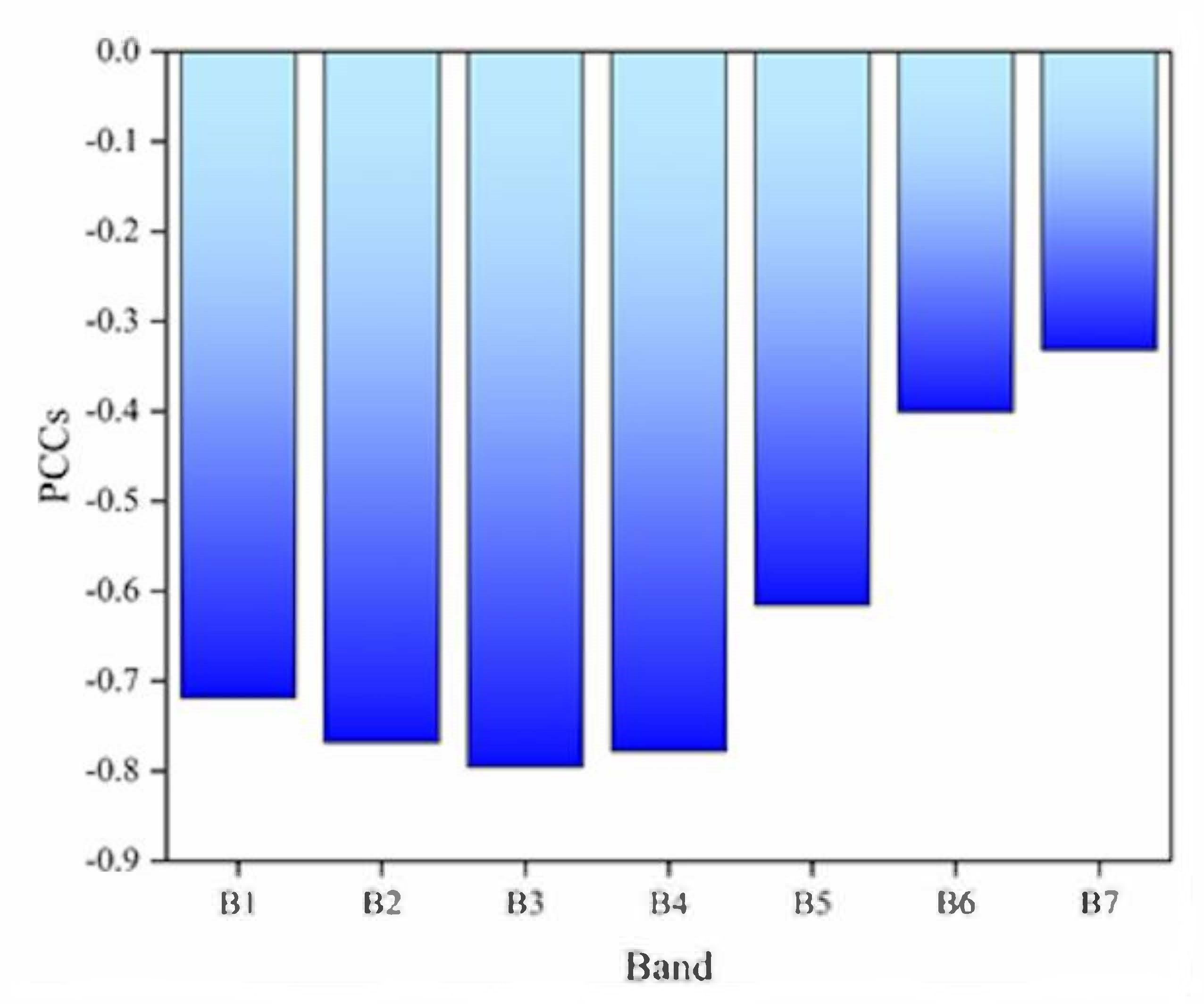
Pearson correlation coefficients between seven single-bands and chlorophyll-a concentration in Figure 3 show that there is a negative correlation between chlorophyll-a concentration and single-band value. In addition, five of the seven single-bands exist strong correlation (0.6 < |PCCs| < 0.8 $0.6<\left|PCCs\right|<0.8$) with chlorophyll-a concentration, and the band with largest correlation is B3 (PCCs $=-$0.7957 $PCCs=-0.7957$). The other two bands are B6 (PCCs $=-$0.4007) and B7 (PCCs $=-$0.3319 $PCCs=-0.3319$) which have a weak correlation with chlorophyll-a concentration. However, the lowest absolute value of correlation is greater than 0.3, which indicates that chlorophyll-a concentration has a certain correlation with the whole seven single bands.

According to the result of Pearson correlation coefficients between multi-band combinations and chlorophyll-a concentration shown in

Table 4. The multi-band combinations and pearson correlation coefficients.

Dual-Band	PCCs	Three-Band	PCCs	Four-Band	PCCs
B2/B1	−0.7952	B2/(B7 + B1)	−0.7703	(B7 − B2)/(B5 − B1)	−0.7632
B7 + B3	−0.7951	B4*(B5 − B3)	−0.7694	(B7 + B2)/(B6 + B1)	−0.7630
B6 + B3	−0.7909	B2/(B6 + B1)	−0.7677	(B7 − B2)/(B6 − B1)	−0.7628
B4 + B3	−0.7869	B4*(B6 − B3)	−0.7673	(B6 + B2)/(B7 + B1)	−0.7603
B7 − B3	−0.7798	B4*(B7 − B3)	−0.7657	(B6 + B4)*(B5 − B3)	−0.7578
B3 + B2	−0.7787	B2*(B5 − B3)	−0.7605	(B7 + B4)*(B5 − B3)	−0.7545
B6 − B3	−0.7721	B3*(B7 − B4)	−0.7567	(B4 + B2)*(B5 − B3)	−0.7525

Note: PCCs is pearson correlation coefficients. When PCCs > 0, the two variables are positively correlated, otherwise they are negatively correlated. And, the larger the absolute value of PCCs, the stronger the correlation between the two variables.

, the absolute value of PCCs corresponding to the selected multi-band combinations are all larger than 0.75, which shows that they all have a strong correlation with chlorophyll-a concentration. Among the band combinations which are retained, B2/B1 has the largest correlation with chlorophyll-a concentration, and its PCCs is −0.7952.

3.2. Multi-Factor Modeling Result

In order to explore a method to accurately reflect the eutrophication status of Donghu Lake, exploratory experiment is carried out to build inversion model by using multiple factors. Twelve machine learning algorithm models for retrieving chlorophyll-a concentration are constructed by combining the three machine learning algorithms and four kinds of multi-factor dataset, respectively.

3.2.1. BPNN Modeling Training and Simulation Result

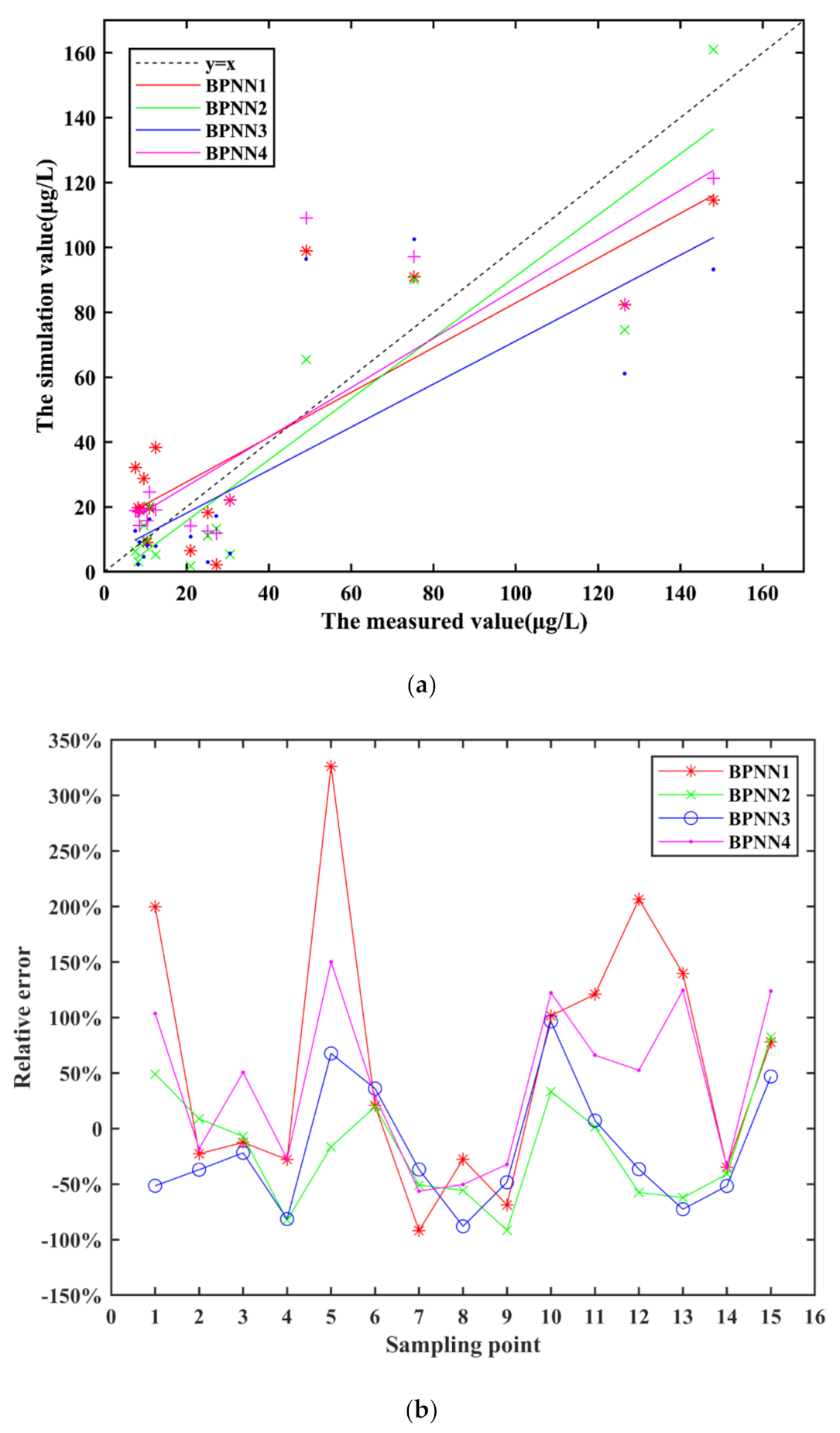
The simulation results of four BPNN models and the measured values of chlorophyll-a concentration are shown in Figure 4a. Compared with other three BPNN models, the simulation results and the measured values of BPNN2 have better fitting effect.

Figure 4b shows the relative error between the simulation results and the measured values, which can be used to compare the effects of these four models. Models in some sample points do not show a good effect, and some simulation results exceed the acceptable range (the relative error is larger than 100%). Among the four BPNN models, the simulation results relative error of single-band model (BPNN1) fluctuate wildly, and the model effect of BPNN1 is not good. There are four sample points where the relative error of the four-band model (BPNN4) are larger than 100%, the model does not perform well. In addition, the simulation results of the other two multi-band models are relatively good. MRE of the four BPNN models can reach 60.51%, −17.97%, −18.08% and 40.26%, respectively. The model of BPNN2 shows the best inversion results, but the error of other model is too large, which shows that the inversion results of multi-factor models built by BPNN can be only for reference.

The same conclusion can be obtained from the determination coefficient of BPNN models in

Table 5. The determination coefficient of BPNN models.

BPNN Model	R1	R2
BPNN1	0.73	0.67
BPNN2	0.82	0.83
BPNN3	0.86	0.83
BPNN4	0.80	0.79

Note: R1 is the determination coefficient of the regression between the training result and the corresponding measured value. R2 is the determination coefficient of the regression between the testing result and the corresponding measured value.

. It shows that R1 and R2 of single-band model (BPNN1) is both smaller than these of multi-band model, and R1 and R2 of BPNN4 is the smallest among the three multi-band models, it demonstrates that BPNN1 and BPNN4 are not effective models for chlorophyll-a inversion.

3.2.2. ELM Modeling Training and Simulation Result

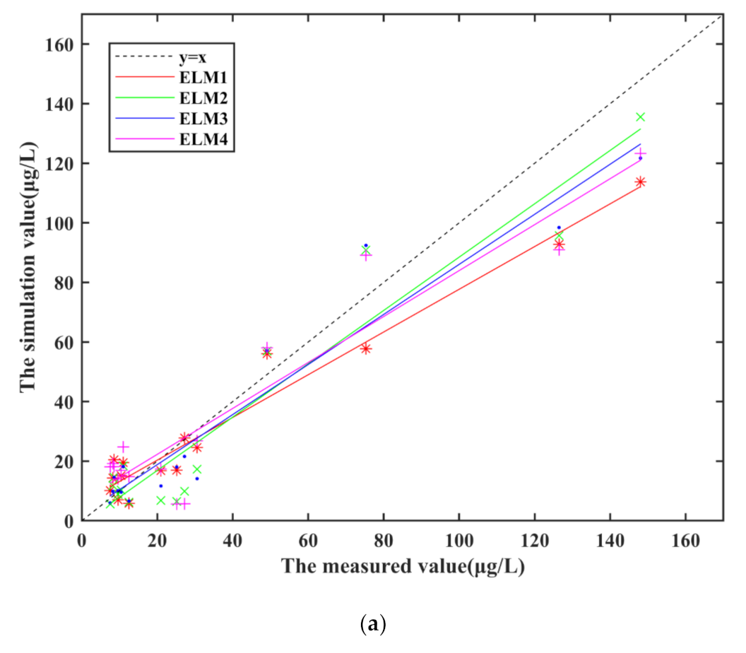
The simulation results of four ELM models and the measured values of chlorophyll-a concentration are shown in Figure 5a. The simulation results of the four ELM models vary with the measured values, and the simulation results of the ELM2 match better with the measured values than other three ELM models.

Although the trend between the simulation results of ELM model and the measured values is relatively consistent, the relative error is quite different, as shown in Figure 5b. The relative error absolute value of the four models is mostly less than 100%, but the relative error at some sampling points exceeds the acceptable range in these four ELM models. These sampling points have the same characteristic that the measured value of chlorophyll-a concentration is small, and small measured values always lead to a phenomenon that the relative error is large although the error is small. MRE of the four ELM models can reach 36.47%, 19.64%, −20.06%, −21.83%, respectively. And, ELM2 is better than other three multi-factor models based on ELM.

The determination coefficient of ELM models is shown in

Table 6. The determination coefficient of ELM models.

ELM Model	R1	R2
ELM1	0.83	0.80
ELM2	0.88	0.84
ELM3	0.85	0.86
ELM4	0.84	0.84

Note: R1 is the determination coefficient of the regression between the training result and the corresponding measured value. R2 is the determination coefficient of the regression between the testing result and the corresponding measured value.

. It can be found that R1 and R2 of the four ELM models are between 0.80 and 0.86, which indicates that the four models are all useful.

3.2.3. SVM Modeling Training and Simulation Result

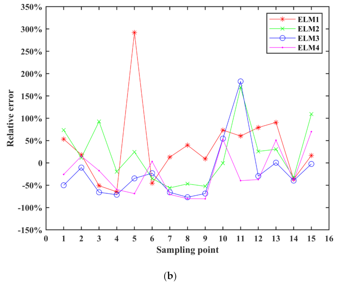
As we can see in Figure 6a, most of the model simulation results of SVM models are in good agreement with the measured values, even though some points with larger measured values.

At the same time, the relative error of the SVM model in Figure 6b is not large in general. Only the relative errors of one point of SVM1 and four points of SVM4 are beyond the acceptable range, but they are all less than 1.5. Furthermore, both SVM2 and SVM3 show good simulation result. MRE of the four SVM models can reach 10.78%, −9.89%, −4.25% and 29.52%, respectively, which achieves a good effect. Compared with other three SVM models, SVM3 work better.

From the

Table 7. The determination coefficient of SVM models.

SVM Model	R1	R2
SVM1	0.84	0.87
SVM2	0.89	0.93
SVM3	0.87	0.93
SVM4	0.85	0.93

Note: R1 is the determination coefficient of the regression between the training result and the corresponding measured value. R2 is the determination coefficient of the regression between the testing result and the corresponding measured value.

, R1 and R2 of four SVM models are all at a high level. The results show that SVM is an effective algorithm to build chlorophyll-a inversion model, and accurate simulation results can be obtained whether using single-band or multi-band combination as influence factors.

3.3. Single-Factor Modeling Result

Single-factor modeling is a commonly used modeling method. In this paper, we use single-factor dataset and three machine learning algorithms to build inversion models, and compare the effects of the three models. Through correlation analysis, B2/B1 is the band combination which has the strongest correlation with chlorophyll-a concentration, PCCS = −0.7952.

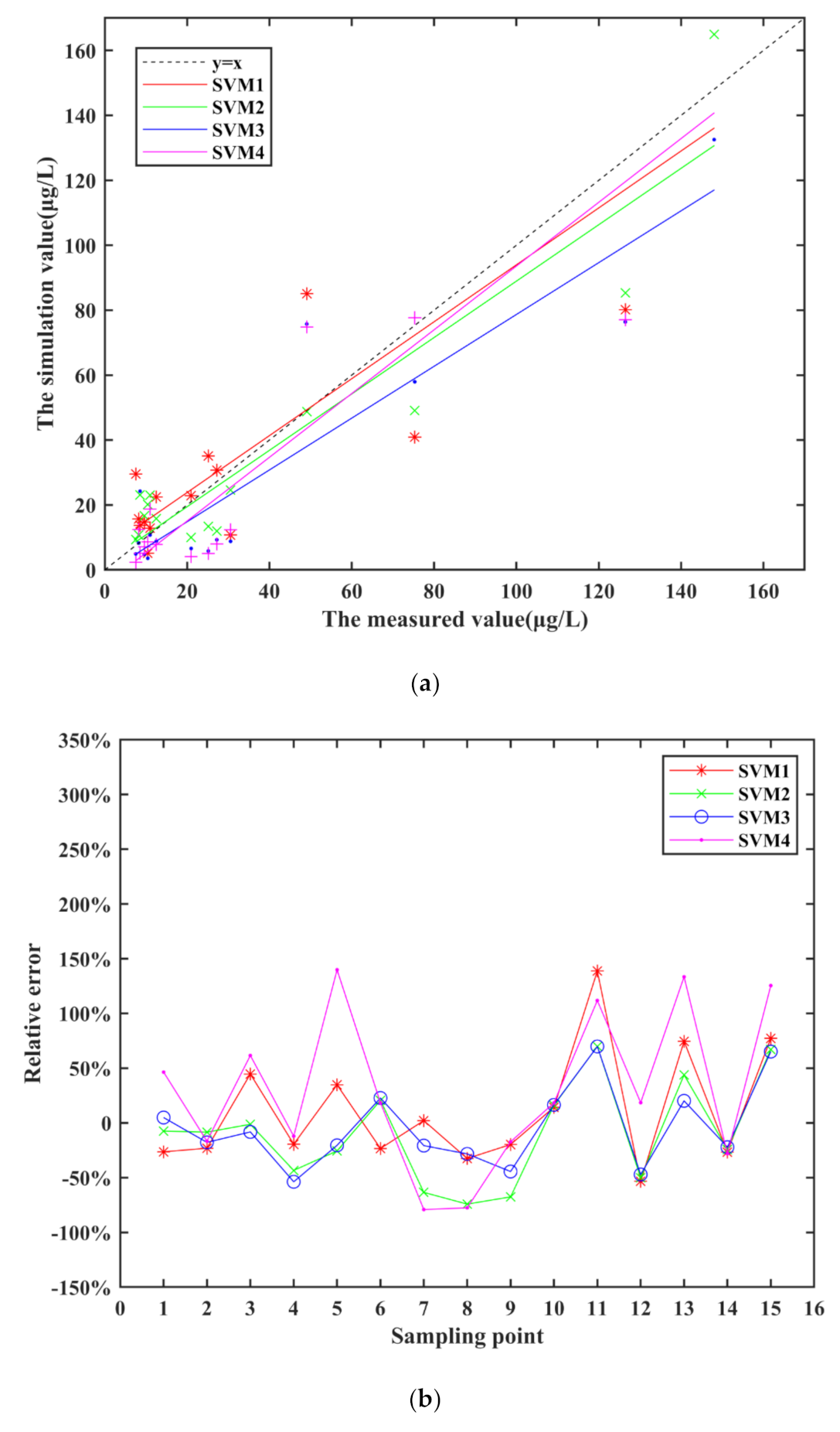
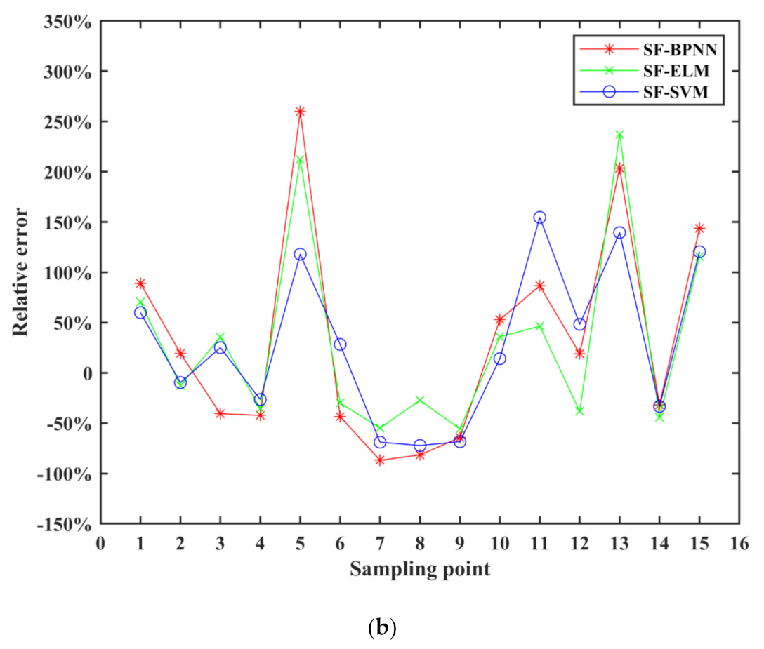
Figure 7a shows the simulation results of three different machine learning algorithm models by using single-factor dataset. The band range of relative error of the three single-factor models between the simulation results and the measured values is relatively large, especially the absolute value of the relative error of the sampling point with larger measured value of chlorophyll-a concentration in Figure 7b. The relative error of SF-SVM is the smallest among the three models, MRE of SF-BPNN, SF-ELM and SF-SVM reached 26.60%, 23.19% and 21.45%, respectively.

Regression analysis was performed on the simulation result and the measured structure in the modeling process of the three single-factor models. The result of R1 and R2 are shown in

Table 8. The determination coefficient of Single-factor models.

Single-Factor Model	R1	R2
SF-BPNN	0.85	0.87
SF-ELM	0.91	0.85
SF-SVM	0.90	0.91

Note: R1 is the determination coefficient of the regression between the training result and the corresponding measured value. R2 is the determination coefficient of the regression between the testing result and the corresponding measured value.

. It can be seen that R1 and R2 of SF-SVM model are higher than other single-factor models, which are 0.90 and 0.91 respectively, and it reflects the SF-SVM simulation result fit well with the measured values.

4. Discussion

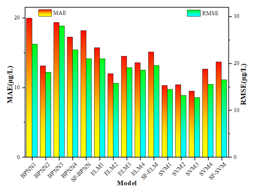
In this study, a variety of chlorophyll-a concentration inversion models were built by combining five kinds of dataset (a single-factor dataset and four kinds of multi-factor dataset) with three machine learning algorithms (BPNN, ELM, SVM). The coefficient of determination, RE, MRE, MAE, RMSE of the training process and test process result in the modeling were used as the evaluation criteria of model accuracy. On this basis, the impacts of single-factor and multi-factor, single-band and multi-band, and three machine learning algorithms on model accuracy were compared and analysed. The Figure 8 uses MAE and RMSE to compare the simulation accuracy of single-factor models and multi-factor models.

4.1. Impacts of Single-Factor and Multi-Factor on Model Accuracy

There are twelve multi-factor models and three single-factor models. Affected by using different algorithms and different band combinations, simulation results of the multi-factor models vary greatly. Because the single-factor models use sample dataset, so they are relatively easy to be built, and the effect of those models is mainly affected by the algorithm. The simulation result show that when the same machine learning algorithm is used, the absolute value of the MRE of the single-factor model is smaller than that of the single-band model, but is not smaller than that of all multi-band models. As we can see, the model simulation results show that BPNN2, ELM2, and SVM3 have the smallest absolute value of MRE among the multi-factor models built by the three algorithms. However, the MRE of SF-BPNN is 26.60%, the RE of BPNN2 is −17.97%. And, the MRE of SF-ELM is 23.19%, the RE of ELM2 is 19.64%. Besides, the MRE of SF-SVM is 21.45%, and the RE of SVM3 is −4.25%.

The same phenomenon happens when the simulation accuracy of the same algorithm model is compared. The MAE and RMSE of SF-BPNN, SF-ELM, SF-SVM are 18.84 μg/L and 27.16 μg/L, 13.81 μg/L and 21.55 μg/L, 11.52 μg/L and 15.90 μg/L, respectively. As the result display the MAE and RMSE of the single-factor model are at the middle level in those models used the same algorithm, in other words, the test result error of the single-factor models is acceptable, but also can be improved. All in all, although single-factor modeling is effective, multi-factor dataset for modeling has the possibility to improve the accuracy of the model, and the multi-factor inversion model is worth exploring and using.

4.2. Impacts of Single-Band and Multi-Band Combinations on Model Accuracy

From the appearance of BPNN1, ELM1 and SVM1, we can find that although there is a certain correlation between chlorophyll-a concentration and seven single bands, the effect is not good when they are used to establish a simple machine learning algorithm inversion model. The simulation result of three single-band models are poorly fitted to the sequence of measured values, and the relative error is also larger than other models as shown. Therefore, in order to improve the inversion accuracy, the band combination is usually used as the influence factor to build the chlorophyll-a concentration inversion model. At the same time, an interesting phenomenon has been discovered that, although the machine learning model constructed by multi-band combinations can improve the simulation effect, it does not mean that the more bands involved in the model construction, the better the model will be. For example, the effect of the models constructed with four-bands is generally worse than that of two-bands models and three-bands models, which is manifested as that four-bands models usually have the characteristics of large relative error and instability. This phenomenon occurs because B6 ($\mathrm{PCCs}=-0.4007$) and B7 ($\mathrm{PCCs}=-0.3319$) have a weak correlation with the concentration of chlorophyll-a, but the combination of bands used for modeling has a strong correlation with the concentration of chlorophyll-a. The multi-band models use band combination as input, which avoids the low correlation between input layer data and chlorophyll-a concentration, so the accuracy of the multi-band is higher than that of the single-band models. However, when multi-band combinations are adopted, more errors will be introduced into the model at the same time. If too many bands are involved in modeling, the superposition of errors will exceed the promotion effect of multi-band, which reduces the accuracy of the model. Therefore, it is necessary to optimize the number of bands used for band combination through multiple training and testing when modeling.

4.3. Impacts of Machine Learning Algorithms on Model Accuracy

The simulation result of multi-band BPNN models show that the BPNN models are available in simulating the area with low chlorophyll-a concentration, but do not perform well at the high concentration area. Therefore, the chlorophyll-a concentration inversion models established by BPNN only have a certain reference value for the inversion of chlorophyll-a concentration in Donghu Lake. The simulation results error of multi-band ELM models is relatively acceptable, and the results are valid for simulating the chlorophyll-a concentration, so ELM can be used as an alternative algorithm for modeling of chlorophyll-a inversion. By compared with the models based on BPNN and ELM, the RE of SVM models are generally smaller, which shows that SVM has an advantage over BPNN and ELM in chlorophyll-a concentration inversion modeling. When MAE and RMSE are analysed to evaluate the accuracy of the model, the similar conclusion can be obtained. When modeling with the same dataset, the MAE and RMSE of the inversion model constructed by SVM are the smallest among the three models using different machine learning algorithms. From the comprehensive performance of each evaluation index, BPNN2 (MRE = −17.97%, R1 = 0.82, R2 = 0.83, MAE = 13.10 μg/L, RMSE = 18.11 μg/L), ELM2 (MRE = 19.64%, R1 = 0.88, R2 = 0.84, MAE = 11.96 μg/L, RMSE = 15.73 μg/L) are the best in BPNN models and ELM models, respectively. However, compared with other models, the evaluation criteria indicate that SVM3 works better (MRE = −4.25%, R1 = 0.87, R2 = 0.93, MAE = 9.44 μg/L, RMSE = 12.66 μg/L). Generally, the model built by SVM with seven three-band combinations as input layer showed the better inversion effect on chlorophyll-a concentration than other multi-factor models. When comparing the chlorophyll-a concentration inversion effect of the three single-factor models, SF-SVM performs the best effects that the MRE, MAE, RMSE of SF-SVM are 26.60%, 18.84 μg/L and 27.16 μg/L, respectively. Therefore, conclusion can be made that the performance of SVM model is better than that of BPNN and ELM model, which is the same as the results of multi-factor models. Combined with the results of multi-factor model and single-factor model, it demonstrates that SVM is more suitable than BPNN and ELM for chlorophyll-a concentration inversion modeling of Donghu Lake.

In this study, the inversion effect of some models are not good, which does not reflect the advantages of the three machine learning algorithms in solving the high-dimensional nonlinear problem of chlorophyll-a concentration remote sensing retrieval simulation. A large part of the reason is that these algorithms are simply used in modeling without any optimization. Therefore, in order to increase the accuracy of machine algorithm retrieval model, methods of optimizing and improving simple machine algorithm modeling deserve to be further explored.

4.4. Analysis of Simulation Result of Chlorophyll-a Concentration

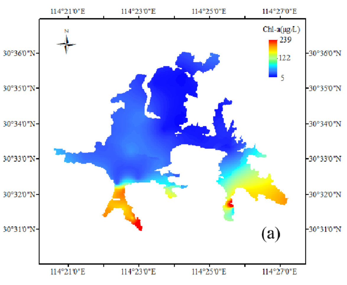
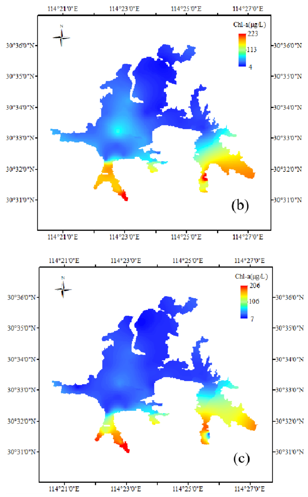
The comparison results show that SVM3 is the most effective multi-factor model for the chlorophyll-a inversion, and the SF-SVM model is the best one among the three single-factor models. In order to obtain the chlorophyll-a concentration distribution status of Donghu Lake, the two models are used to simulate the chlorophyll-a concentration distribution of the whole Donghu Lake on 17 December 2017. Figure 9a–c are the measured value of chlorophyll-a concentration distribution map, the SVM3 simulation value distribution map, the SF-SVM simulation value distribution map.

From the three maps, the simulation value of chlorophyll-a concentration distribution maps is similar with the measured value on the whole. On 17 December 2017, the areas with high chlorophyll-a concentration distributed in Miaohu Lake, Houhu Lake, Yujia Lake and Lingjiao Lake, and some of areas were seriously eutrophicated. Guozheng Lake and Tangling Lake have the largest water area in all the sub lakes of Donghu Lake, and they have better water quality and chlorophyll-a concentration is relatively low. It shows that the simulation results are generally consistent with the actual situation of Donghu Lake. However, there are some difference in local areas between the three maps. In general, SVM3 simulation value of chlorophyll-a concentration distribution map (in Figure 9b) are more similar with measured value of chlorophyll-a concentration distribution map (in Figure 9a). On the one hand, the range of SVM3 simulation value of chlorophyll-a concentration distribution is closer to measured value of chlorophyll-a concentration distribution, and the SVM3 simulation value have a smaller deviation from measured value compared to the SVM3 simulation value. On the other hand, the concentration of chlorophyll-a in the northeast corner of the Yujia Lake is very high, both the Figure 9a,b have showed this phenomenon, it indicates that SVM3 model can better show the distribution of chlorophyll-a in detail. In summary, the simulation effect of SVM3 is better than that of SF-SVM.

Both the three maps reflect that the concentration of chlorophyll-a in Miaohu Lake, Houhu Lake, Yujia Lake and Lingjiao Lake is very high. The three lakes have the same geographical location characteristic that they are all located near densely populated areas, such as schools, residential areas and scenic spots, and they all have a small area, a long coastline, sluggish flow. They receive a large amount of domestic sewage containing nitrogen and phosphorus from the surrounding sewage outlets, however, the pollutants are not easy to diffuse and transfer, which leads to serious local eutrophication. The Houhu Lake is relatively large, but the lake has shallow water level, many bays, long shorelines, and dense surrounding residents. In addition, a large amount of domestic sewage and farmland irrigation wastewater are discharged into the lake, which leads to non-point source pollution and a heavy eutrophication load. Therefore, the concentration of chlorophyll-a in these lakes is relatively high. However, the chlorophyll-a concentration distribution map also has some parts that are not completely consistent with the actual situation of Donghu Lake. For example, the water quality of Shuiguo Lake and the southwest coast of Guozheng Lake have been eutrophic affected by the surrounding environment, and it has not been reflected in the distribution maps. This is mainly due to our insufficient number of sampling points, and most of the sampling points are set in the area with good water quality where are far from the shore.

5. Conclusions

In this study, fifteen kinds of chlorophyll-a concentration inversion models were constructed by three different machine learning algorithms (BPNN, ELM and SVM) and five kinds of dataset. RE, MRE, R, MAE, RMSE were adopted to compare and analyse inversion model accuracy. The conclusions can be drawn as follows:

(1)

Although the single-factor modeling is effective, some multi-factor models work better than single-factor models, so multi-factor dataset for modeling has the possibility to improve the accuracy of the model, and the multi-factor inversion model is worth exploring and using.

(2)

As the influence factors, seven band combinations are better than seven single bands when modeling. It is not that the more bands involved for modeling, the better the accuracy of the model. Therefore, the number of bands should be optimized to build band combination.

(3)

SVM is more suitable than BPNN and ELM for chlorophyll-a concentration inversion modeling of Donghu Lake. SVM3 (the model built by SVM with seven three-band combinations and chlorophyll-a concentration as dataset) showed the best inversion effect on chlorophyll-a concentration among all multi-factor models that the MRE, MAE, RMSE of SF-SVM are 30.82%, 9.44 μg/L and 12.66 μg/L, respectively. SF-SVM performs a better effect on the inversion of chlorophyll-a concentration than SF-BPNN and SF-ELM, the MRE, MAE, RMSE of SF-SVM are 28.63%, 13.69 μg/L and 16.49 μg/L, respectively.

(4)

The simulation result are generally consistent with the actual situation of Donghu Lake, and different in some local areas with the measured distribution from the three maps. And, the simulation effect of SVM3 is better than that of SF-SVM. The chlorophyll-a concentration in some sub lakes of Donghu Lake is very high, which is related to their geographical location characteristic and influenced by the human activity around them. Besides, the chlorophyll-a concentration distribution map also has some parts that are not completely consistent with the actual situation of Donghu Lake, and this is mainly due to the insufficient number of sampling points.

Furthermore, on the basis of the current research, we try to optimize and improve the machine learning algorithm, deeply analyze the spatiotemporal heterogeneity of chlorophyll-a concentration remote sensing inversion, and build a portable and universal inversion model for continuous and prolonged monitoring of chlorophyll-a.

References

- Chakrabarti, S. Eutrophication—A Global Aquatic Environmental Problem: A Review. Res. Rev. J. Ecol. Environ. Sci. 2018, 6, 1–6. [Google Scholar]
- de Jonge, V.N.; Elliott, M.; Orive, E. Causes, historical development, effects and future challenges of a common environmental problem: Eutrophication. Hydrobiologia 2002, 475, 1–19. [Google Scholar] [CrossRef]
- Qin, B.; Gao, G.; Zhu, G.; Zhang, Y.; Song, Y.; Tang, X.; Hai, X.; Deng, J. Lake eutrophication and its ecosystem response. Chin. Sci. Bull. 2013, 58, 961–970. [Google Scholar] [CrossRef] [Green Version]
- Kudela, R.M.; Palacios, S.L.; Austerberry, D.C.; Accorsi, E.K.; Guild, L.S.; Torres-Perez, J. Application of hyperspectral remote sensing to cyanobacterial blooms in inland waters. Remote Sens. Environ. 2015, 167, 196–205. [Google Scholar] [CrossRef] [Green Version]
- Mulia, I.E.; Tay, H.; Roopsekhar, K.; Tkalich, P. Hybrid ANN-GA model for predicting turbidity and chlorophyll-a concentrations. AOGS 8th annual meeting and geosciences. World Community Exhib. 2013, 7, 279–299. [Google Scholar]
- He, J.; Chen, Y.; Wu, J.; Stow, D.A.; Christakos, G. Space-Time Chlorophyll-a Retrieval in Optically Complex Waters that Accounts for Remote Sensing and Modeling Uncertainties and Improves Remote Estimation Accuracy. Water Res. 2020, 171, 1–17. [Google Scholar] [CrossRef] [PubMed]
- Gevorgyan, G.; Rinke, K.; Schultze, M.; Mamyan, A.; Kuzmin, A.; Belykh, O.; Sorokovikova, E.; Hayrapetyan, A.; Hovsepyan, A.; Khachikyan, T.; et al. First report about toxic cyanobacterial bloom occurrence in Lake Sevan, Armenia. Int. Rev. Hydrobiol. 2020, 105, 131–142. [Google Scholar] [CrossRef]
- Papenfus, M.; Schaeffer, B.; Pollard, A.I.; Loftin, K. Exploring the potential value of satellite remote sensing to monitor chlorophyll-a for US lakes and reservoirs. Environ. Monit. Assess. 2020, 192, 808. [Google Scholar] [CrossRef] [PubMed]
- Xiang, X.; Lu, W.; Cui, X.; Li, Z.; Tao, J. Simulation of Remote-Sensed Chlorophyll Concentration with a Coupling Model Based on Numerical Method and CA-SVM in Bohai Bay, China. J. Coast. Res. 2018, 84, 1–9. [Google Scholar] [CrossRef]
- Kuhn, C.; Valerio, A.D.; Ward, N.; Loken, L.; Sawakuchi, H.O.; Karnpel, M.; Richey, J.; Stadler, P.; Crawford, J.; Striegl, R.; et al. Performance of Landsat-8 and Sentinel-2 surface reflectance products for river remote sensing retrievals of chlorophyll-a and turbidity. Remote Sens. Environ. 2019, 224, 104–118. [Google Scholar] [CrossRef] [Green Version]
- Rodriguez-Lopez, L.; Duran-Llacer, I.; Gonzalez-Rodriguez, L.; Abarca-del-Rio, R.; Cardenas, R.; Parra, O.; Martinez-Retureta, R.; Urrutia, R. Spectral analysis using LANDSAT images to monitor the chlorophyll-a concentration in Lake Laja in Chile. Ecol. Inform. 2020, 60, 101183. [Google Scholar] [CrossRef]
- Vanhellemont, Q.; Ruddick, K. Advantages of high quality SWIR bands for ocean colour processing: Examples from Landsat-8. Remote Sens. Environ. 2015, 161, 89–106. [Google Scholar] [CrossRef] [Green Version]
- Sun, D.; Li, Y.; Wang, Q. A Unified Model for Remotely Estimating Chlorophyll a in Lake Taihu, China, Based on SVM and In Situ Hyperspectral Data. IEEE Trans. Geosci. Remote Sens. 2009, 47, 2957–2965. [Google Scholar]
- Carder, K.L.; Chen, F.R.; Cannizzaro, J.P.; Campbell, J.W.; Mitchell, B.G. Performance of the MODIS semi-analytical ocean color algorithm for chlorophyll-a. Adv. Space Res. 2004, 33, 1152–1159. [Google Scholar] [CrossRef]
- Hassani, M.; Chabou, M.C.; Hamoudi, M.; Guettouche, M.S. Index of extraction of water surfaces from Landsat 7 ETM+ images. Arab. J. Geosci. 2015, 8, 3381–3389. [Google Scholar] [CrossRef]
- Chen, Q.; Huang, M.; Bai, K.; Li, X. An Optimal Two Bands Ratio Model to Monitor Chlorophyll-a in Urban Lake Using Landsat 8 Data. E3S Web Conf. 2020, 143, 02003. [Google Scholar] [CrossRef] [Green Version]
- Lesht, B.M.; Barbiero, R.P.; Warren, G.J. Verification of a simple band ratio algorithm for retrieving Great Lakes open water surface chlorophyll concentrations from satellite observations. J. Great Lakes Res. 2015, 42, 448–454. [Google Scholar] [CrossRef]
- Murugan, P.; Sivakumar, R.; Pandiyan, R.; Annadurai, M. Performance Comparison of Band Ratio and Derivative Ratio Algorithms in Chlorophyll-A Estimation using Hyperspectral Data. Int. J. Earth Sci. Eng. 2016, 9, 347–352. [Google Scholar]
- Lary, D.J.; Alavi, A.H.; Gandomi, A.H.; Walker, A.L. Machine learning in geosciences and remote sensing. Geosci. Front. 2016, 7, 3–10. [Google Scholar] [CrossRef] [Green Version]
- Pyo, J.C.; Duan, H.; Baek, S.; Kim, M.S.; Jeon, T.; Kwon, Y.S.; Lee, H.; Cho, K.H. A convolutional neural network regression for quantifying cyanobacteria using hyperspectral imagery. Remote Sens. Environ. 2019, 233, 111350. [Google Scholar] [CrossRef]
- Singh, A.; Thakur, N.; Sharma, A. A review of supervised machine learning algorithms. In Proceedings of the 2016 3rd International Conference on Computing for Sustainable Global Development (INDIACom), New Delhi, India, 16–18 March 2016; IEEE: New York, NY, USA, 2016; pp. 1310–1315. [Google Scholar]
- Blix, K.; Eltoft, T. Machine Learning Automatic Model Selection Algorithm for Oceanic Chlorophyll-a Content Retrieval. Remote Sens. 2018, 10, 775. [Google Scholar] [CrossRef] [Green Version]
- Jimeno-Saez, P.; Senent-Aparicio, J.; Cecilia, J.M.; Perez-Sanchez, J. Using Machine-Learning Algorithms for Eutrophication Modeling: Case Study of Mar Menor Lagoon (Spain). Int. J. Environ. Res. Public Health 2020, 17, 1189. [Google Scholar] [CrossRef] [Green Version]
- Abba, S.I.; Hadi, S.J.; Abdullahi, J. River water modelling prediction using multi-linear regression, artificial neural network, and adaptive neuro-fuzzy inference system techniques. Procedia Comput. Sci. 2017, 120, 75–82. [Google Scholar] [CrossRef]
- Lu, F.; Chen, Z.; Liu, W.; Shao, H. Modeling chlorophyll-a concentrations using an artificial neural network for precisely eco-restoring lake basin. Ecol. Eng. 2016, 95, 422–429. [Google Scholar] [CrossRef]
- Canziani, G.; Ferrati, R.; Marinelli, C.; Dukatz, F. Artificial neural networks and remote sensing in the analysis of the highly variable pampean shallow lakes. Math. Biosci. Eng. 2008, 5, 691–711. [Google Scholar]
- Wang, T.; Tan, C.; Chen, L.; Tsai, Y. Applying Artificial Neural Networks and Remote Sensing to Estimate Chlorophyll-a Concentration in Water Body. In 2008 Second International Symposium on Intelligent Information Technology Application; IEEE: New York, NY, USA, 2008; pp. 540–544. [Google Scholar]
- Cao, Z.; Ma, R.; Duan, H.; Pahlevan, N.; Melack, J.; Shen, M.; Xue, K. A machine learning approach to estimate chlorophyll-a from Landsat-8 measurements in inland lakes. Remote Sens. Environ. 2020, 248, 111974. [Google Scholar] [CrossRef]
- Su, J.; Wang, X.; Zhao, S.; Chen, B.; Li, C.; Yang, Z. A Structurally Simplified Hybrid Model of Genetic Algorithm and Support Vector Machine for Prediction of Chlorophyll a in Reservoirs. Water 2015, 7, 1610–1627. [Google Scholar] [CrossRef] [Green Version]
- Xue, L.; Sha, J.; Wang, Z. Chlorophyll-A Prediction of Lakes with Different Water Quality Patterns in China Based on Hybrid Neural Networks. Water 2017, 9, 524. [Google Scholar]
- Zhang, T.; Huang, M.; Wang, Z. Estimation of Chlorophyll-a Concentration of Lakes Based on SVM Algorithm and Landsat 8 OLI Images. Environ. Sci. Pollut. Res. 2020, 27, 14977–14990. [Google Scholar] [CrossRef]
- Li, X.; Huang, M.; Wang, R. Numerical Simulation of Donghu Lake Hydrodynamics and Water Quality Based on Remote Sensing and MIKE 21. ISPRS Int. J. Geo-Inf. 2020, 9, 94. [Google Scholar] [CrossRef] [Green Version]
- Yang, X.; Jiang, Y.; Deng, X.; Zheng, Y.; Yue, Z. Temporal and Spatial Variations of Chlorophyll a Concentration and Eutrophication Assessment (1987–2018) of Donghu Lake in Wuhan Using Landsat Images. Water 2020, 12, 2192. [Google Scholar] [CrossRef]
- Palmer, S.C.J.; Kutser, T.; Hunter, P.D. Remote sensing of inland waters: Challenges, progress and future directions. Remote Sens. Environ. 2014, 157, 1–8. [Google Scholar] [CrossRef] [Green Version]
- Keller, P.A. Comparison of two inversion techniques of a semi-analytical model for the determination of lake water constituents using imaging spectrometry data. Sci. Total Environ. 2001, 268, 189–196. [Google Scholar] [CrossRef]
- Yun, X.; Yang, Y.; Liu, M.; Zhang, M.; Wang, J. Distribution, Seasonal Variations, and Ecological Risk Assessment of Polycyclic Aromatic Hydrocarbons in the East Lake, China. CLEAN-Soil Air Water 2016, 44, 506–514. [Google Scholar] [CrossRef]
- Wang, T.; Wang, Q.; Xia, S.; Yan, C.; Pei, G. Response of benthic algae to environmental conditions in an urban lake recovered from eutrophication, China. J. Oceanol. Limnol. 2020, 38, 93–101. [Google Scholar] [CrossRef]
- Chen, Q.; Huang, M.; Tang, X. Eutrophication assessment of seasonal urban lakes in China Yangtze River Basin using Landsat 8-derived Forel-Ule index: A six-year (2013–2018) observation. Sci. Total Environ. 2019, 745, 135392. [Google Scholar] [CrossRef] [PubMed]
- Boucher, J.; Weathers, K.C.; Norouzi, H.; Steele, B. Assessing the effectiveness of Landsat 8 chlorophyll a retrieval algorithms for regional freshwater monitoring. Ecol. Appl. 2018, 28, 1044–1054. [Google Scholar] [CrossRef] [PubMed] [Green Version]
- Rumelhart, D.E.; Hinton, G.E.; Williams, R.J. Learning representations by back-propagating errors. Nature 1986, 323, 533–536. [Google Scholar] [CrossRef]
- Shao, D.; Nong, X.; Tan, X.; Chen, S.; Xu, B.; Hu, N. Daily water quality forecast of the south-to-north water diversion project of China based on the cuckoo search-back propagation neural network. Water 2018, 10, 1471. [Google Scholar] [CrossRef] [Green Version]
- Goh, A.T.C. Back-Propagation Neural Networks for Modeling Complex Systems. Artif. Intell. Eng. 1995, 9, 143–151. [Google Scholar] [CrossRef]
- Chen, N.; Xiong, C.; Du, W.; Wang, C.; Lin, X.; Chen, Z. An Improved Genetic Algorithm Coupling a Back-Propagation Neural Network Model (IGA-BPNN) for Water-Level Predictions. Water 2019, 11, 1795. [Google Scholar] [CrossRef] [Green Version]
- Zhu, Y.; Zhu, L.; Li, J.; Chen, Y.; Zhang, Y.; Hou, H.; Ju, X.; Zhang, Y. The study of inversion of chlorophyll a in Taihu based on GF-1 WFV image and BP neural network. Acta Sci. Circumstantiae 2017, 37, 130–137. [Google Scholar]
- Zhang, Q.; Wu, Z.; Xie, X. Research progress of the inversion algorithm of chlorophyll-a concentration in estuaries and coastal waters. Ecol. Sci. 2017, 36, 215–222. [Google Scholar]
- Zhang, X.; Zheng, X. Discussion on Retrieval Method of Surface Chlorophyll Concentration of the Bohai Bay Based on BP Neural Network. J. Ocean Technol. 2018, 37, 79–87. [Google Scholar]
- Nazeer, M.; Bilal, M.; Alsahli, M.M.; Shahzad, M.I.; Waqas, A. Evaluation of empirical and machine learning algorithms for estimation of coastal water quality parameters. ISPRS. Int. J. Geo-Inf. 2017, 6, 360. [Google Scholar] [CrossRef] [Green Version]
- Jiang, B.; Liu, H.; Xing, Q.; Cai, J.; Zheng, X.; Li, L.; Liu, S.; Zheng, Z.; Xu, H.; Meng, L. Evaluating Traditional Empirical Models and BPNN Models in Monitoring the Concentrations of Chlorophyll-A and Total Suspended Particulate of Eutrophic and Turbid Waters. Water 2021, 13, 650. [Google Scholar] [CrossRef]
- Huang, G.; Zhu, Q.; Siew, C. Extreme learning machine: A new learning scheme of feedforward neural networks. In Proceedings of the International Joint Conference on Neural Networks (IJCNN), Budapest, Hungary, 25–29 July 2004; IEEE: New York, NY, USA, 2004; Volume 2, pp. 985–990. [Google Scholar]
- Wei, Y.; Huang, H.; Chen, B.; Zheng, B.; Wang, Y. Application of Extreme Learning Machine for Predicting Chlorophyll-a Concentration Inartificial Upwelling Processes. Math. Probl. Eng. 2019, 2019, 1–11. [Google Scholar] [CrossRef] [Green Version]
- Ding, S.; Xu, X.; Nie, R. Extreme learning machine and its applications. Neural Comput. Appl. 2014, 25, 549–556. [Google Scholar] [CrossRef]
- Fan, G.; Cao, H.; Xu, J. Prediction of chlorophyll a in Taihu Lake based on HJ-1A CCD imagery and ELM model. J. Water Resour. Water Eng. 2020, 31, 16–22. [Google Scholar]
- Huang, H.; Zheng, B.; Wang, Y.; Wei, Y. Wavelet Neural Network for Modeling Chlorophyll a Concentration Affected by Artificial Upwelling. Sci. World J. 2019, 2019, 4590981. [Google Scholar] [CrossRef]
- Vapnik, V.N. The Nature of Statistical Learning Theory. IEEE Trans. Neural Netw. 1997, 8, 1564. [Google Scholar]
- Bangira, T.; Alfieri, S.M.; Menenti, M.; Niekerk, A.V.; van Niekerk, A. Comparing Thresholding with Machine Learning Classifiers for Mapping Complex Water. Remote Sens. 2019, 11, 1351. [Google Scholar] [CrossRef] [Green Version]
- Kong, X.; Che, X.; Su, R.; Zhang, C.; Yao, Q.; Shi, X. A new technique for rapid assessment of eutrophication status of coastal waters using a support vector machine. J. Oceanol. Limnol. 2018, 36, 59–72. [Google Scholar] [CrossRef]
- Peterson, K.T.; Sagan, V.; Sidike, P.; Hasenmueller, E.A.; Sloan, J.J.; Knouft, J.H. Machine Learning-Based Ensemble Prediction of Water-quality Variables Using Feature-level and Decision-level Fusion with Proximal Remote Sensing. Photogramm. Eng. Remote Sens. 2019, 85, 269–280. [Google Scholar] [CrossRef]
- Xu, Y.; Ma, C.; Liu, Q.; Xi, B.; Qian, G.; Zhang, D.; Huo, S. Method to predict key factors affecting lake eutrophication–A new approach based on Support Vector Regression model. Int. Biodeterior. Biodegrad. 2015, 102, 308–315. [Google Scholar] [CrossRef]
- Qian, X.; Qian, Y.; Liu, J.; Kong, X. Application of SVM on Chl-a concentration retrievals in Taihu Lake. China Environ. Sci. 2009, 29, 78–83. [Google Scholar]
- Li, X.; Su, R.; Zhang, C.; Shi, X. A Chl-a Prediction Model Based on Support Vector Machine in Yangtze River A Chl-a Prediction Model Based on Support Vector Machine in Yangtze River. Period. Ocean. Univ. China 2019, 49, 69–76. [Google Scholar]
- Alizamir, M.; Heddam, S.; Kim, S.; Mehr, A.D. On the implementation of a novel data-intelligence model based on extreme learning machine optimized by bat algorithm for estimating daily chlorophyll-a concentration: Case studies of river and lake in USA. J. Clean. Prod. 2020, 285, 124868. [Google Scholar] [CrossRef]
Figure 1.
The map of China (a), the map of Hubei Province (b) and the sampling points distribution in Donghu Lake (c).
Figure 2.
The research flow chart of machine learning algorithm modeling and chlorophyll-a concentration inversion.
Figure 3.
The single bands and pearson correlation coefficients.
Figure 4.
Modeling simulation results (a) and relative error (b) of BPNN models.
Figure 5.
Modeling simulation results (a) and relative error (b) of ELM models.
Figure 6.
Modeling simulation results (a) and relative error (b) of SVM models.
Figure 7.
Modeling simulation results (a) and relative error (b) of Single-factor models.
Figure 8.
Simulation accuracy evaluation comparison of each model.
Figure 9.
Comparison of the observed value (a), the SVM3 simulation value (b) and the SF-SVM simulation value (c) of chlorophyll-a concentration distribution map.