The Effect of Social Behavior on Residential Water Consumption

Abstract

We analyze how residential water consumption is influenced by the consumption of households belonging to the same social group (peer effect). Analyses are based on household-level data provided by the Brazilian Household Budget Survey and use an innovative strategy that estimates the spatial dependence of water consumption while simultaneously controlling for potential sources of sample selectivity and endogeneity. The estimates of our quantile regression models highlight that, conditional on household characteristics, the greater the household water consumption, the greater the peer effect. In other words, the overconsumption of residential water seems to be influenced mainly by the behavior of social peers.

1. Introduction

Water demand has overgrown and placed increasing pressure on the limited global water supply suitable for human consumption [1]. Understanding the factors influencing water demand—particularly overconsumption—has become a central priority for managing water resources and economic development [2,3]. Although population growth and income growth are critical factors for understanding water demand [4], social behavior also plays a central role in individual demand [5]. The influence of peers on private goods consumption has gained increasing attention in the economics literature [6]. However, only a few studies have evaluated the effects of peers on the consumption of environmental goods and services.

The classic studies by Schelling [7,8] highlight how regular or sporadic interactions with peers may influence individuals’ economic decisions. These interactions occur through social networks that generate externalities where a reference group’s decisions or actions affect individual preferences [9]. The effect of the reference group may also provide a broader and potentially more accurate explanation of variations in water consumption [10]. Prior studies have already shown spatial dependence patterns in water consumption [11], which may also result from peer effects between consumption units in proximity to one another.

Our study analyzes the effects of social behavior on urban residential water consumption. Specifically, we examine how household water consumption is influenced by the water consumption of households in the same neighborhood. Our first hypothesis is that water consumption may reflect social habits and environmental attitudes, such as conscious consumption, cleaning habits, and environmental sustainability concerns. Our second hypothesis is that water consumption may be related to the consumption of positional goods, such as having a swimming pool or a large personal green space (yards or flower gardens). Specifically, we check the extent to which the peer effect may be stronger among those who overuse water for their social standards. In this respect, we check if the peer effect on the water consumption is also related to conspicuous consumption, i.e., the consumption of water in greater quantity than may be considered necessary to cover basic needs.

Our analyses are based on household data from the 2008–2009 Household Budget Survey (POF, Pesquisa de Orçamentos Familiares) of the Brazilian Institute of Geography and Statistics (IBGE, Instituto Brasileiro de Geografia e Estatística). We analyze São Paulo’s (SP) case, the most populous and wealthiest state in Brazil, which already faces challenges related to managing water resources in the country [12]. We use conditional quantile regression models to compare the impacts of peer behavior on the water consumption of different consumption levels within the same social group. We adopt an innovative empirical strategy that simultaneously controls two central problems associated with estimating the function for residential water consumption: sample selection bias in the reports of residential water consumption, and potential endogeneity of the water price and consumption in the neighborhood.

Two main factors can guide the social effect of peers on residential water consumption. The first is associated with the fact that water prices are largely subsidized in many countries, including Brazil, which places this environmental good on the line between public and private goods/services. As a result, individuals may be encouraged to increase their consumption if they realize that their peers consume more water than they do. This hypothesis is related to “the tragedy of the commons,” which was used by Hardin [13] to justify that peer consumption could pressure the supply of natural resources in the medium and long terms. The second factor is that water consumption may be associated with unobservable behavioral practices and social patterns, mainly defined by the reference social group, such as the use of water-saving products and water conservation habits.

The results of this research bring important elements to guide policies for the sustainable use of environmental resources. Above all, our results raise questions on the effectiveness of public policies based on price as the primary mechanism to induce the rational use of water. Public interventions based on behavioral economics could be implemented to create the right incentives and induce, through peer effects, more efficient use of water resources.

2. Literature Review

2.1. Relative Consumption and Social Dependence

Traditional microeconomics characterizes individuals as rational agents whose decisions aim to maximize utility and minimize costs [14]. One central assumption in this analysis is that individuals individually and independently define their preferences, i.e., they maximize the satisfaction of their choices based on their preferences [15]. As a result, individuals’ satisfaction with their consumption would solely depend on their absolute consumption levels. Meanwhile, relative consumption, i.e., the individual’s consumption in relation to the others, would not influence personal well-being [16,17].

More recently, studies from the interface between economics, sociology, and psychology provided broader evidence that human behavior is influenced by comparisons with social peers [18]. Recent developments in behavioral economics, for example, have emphasized the importance of social interactions and hierarchy for the well-being of individuals [19,20,21,22]. Specifically, the satisfaction of people increases (or decreases) when they consume more (or less) than their peers [23,24]. Social relationships and comparisons, particularly among relatively close individuals, would affect the consumption of goods or services. In this respect, economic models’ ability to predict individual preferences would improve significantly with the inclusion of social influence or relative position [5,25].

A critical element of this analysis is the difference between positional and nonpositional goods [16,26]. While the utility of positional goods strongly depends on how individuals compare their consumption levels with others, the utility of nonpositional goods fundamentally depends on individuals’ consumption levels. According to Frank [16,17] and Carlsson et al. [23], the more readily observable or visible to others the goods or services are, the more dependent consumption is on comparisons (and thus the more positional the good). In this respect, the visibility of positional goods is essential for signaling the individual’s consumption status [26].

Social interactions lead to the emulation of behaviors among individuals of the same social group. People may believe that others’ behavior reflects information that they do not have, as they may also interpret others’ decisions or choices as part of a social norm to which they must conform [27]. Relative consumption may also be a result of the pursuit of social status. Veblen’s [28] prominent analysis highlighted the lower classes’ desire to emulate the upper class’s consumption patterns and attitudes, which led to the consumption of goods to display wealth and income rather than cover actual needs (conspicuous consumption). Hirsch [29] argued that the larger the consumption level, the higher the share of consumption related to relative and social status. In other words, once basic needs are met, individuals tend to refocus their decisions on goods and services that provide prestige, distinction, and social status [30].

Relative consumption has become a fundamental component of social relationships and consumption levels, providing essential elements for understanding residential water demand. Understanding the role of relative consumption in water demand could inform water resource policies. It would imply that social behavior changes may be a virtual channel for curbing excessive and unsustainable consumption levels.

2.2. The Determinants of Residential Water Consumption

One primary debate in the analysis of water consumption is whether consumers react more to marginal price (the price of an additional unit of consumption within a block interval) or to the average price (the total cost of water consumed divided by the total volume of consumption) when faced with block tariff. Most studies indicate that the average price appears to be a fair proxy for the perceived price because consumers have difficulty understanding a complicated block tariff structure [31]. For example, Ito [32] found evidence that consumers respond better to the average consumer price than the marginal price. Foster and Beattie [33] suggested that the marginal price would only be recommended in the case of well-informed consumers. In turn, Arbúes et al. [34] suggested that the choice between marginal and average price would not substantially affect price consumption elasticities in water demand functions.

Other studies have focused on the price elasticity and income elasticity of water demand [35]. Studies published through the 1970s assumed that public utility services did not respond to price variation [34]. Since the 1990s, studies have found strong evidence that residential water consumption does respond to price changes, despite its inelasticity of demand [34]. Deyà-Tortella et al. [36] corroborated that domestic water demand is inelastic and may generally depend on other factors, such as household characteristics. Similarly, water demand also appears to be inelastic to income changes [37]. Other important determinants of water consumption include demographic characteristics, infrastructure, weather conditions, family composition, and household infrastructure [37].

More recently, studies inspired by behavioral and environmental economics have analyzed the role of relative consumption in residential water demand [38]. Datta et al. [39] tested the impact of a set of water consumption strategies in Belen, Costa Rica. Based on comparisons of consumption between households and their neighbors, the authors concluded that the most effective interventions influence a particular social behavior. Similarly, Peschiera et al. [40] showed that the rational use and conservation of public services could be improved by providing individuals with information regarding others’ consumption (social network). Brent et al. [41] highlighted that social comparisons could provide a type of tariff or moral persuasion for the rational consumption of a natural resource. The effects of social comparisons on water consumption may also depend on the level of cohesion or proximity between individuals within a social group [42]. According to Peschiera and Taylor [43], the more people identify with their peers, the more likely they are to align their water consumption with their reference group.

Schultz et al. [44] highlighted that households that receive information on their absolute and relative water consumption (consumption relative to their neighbors) consumed less water than their randomized control peers. The authors concluded that individuals are particularly susceptible to social normative information, which becomes a decision-making guide. Schultz et al. [45] also highlighted that normative messages might generate mixed results: decreasing water consumption when the households consume above the average and increasing water consumption when the households consume below the average. Ayres et al. [46] observed that individuals reorganize their preferences and motivations on learning about their peers’ consumption levels.

In summary, information on peer behavior may provide valuable insights into the effectiveness of interventions designed to manage water consumption [47]. Aitken et al. [48] drew similar conclusions, arguing that experience based on strong incentives and well-targeted information is an effective method for inducing significant water consumption changes. The persistence of such interventions may also depend on the social context. Kaaukauskas et al. [49] suggested that we cannot ensure the impact of such interventions over time because people are more drawn to short-term effects. However, Allcott and Rogers [50] provided evidence that these interventions may result in persistent individual behavior changes.

3. Material and Methods

3.1. Variables and Model Specifications

We use a sample of 3623 households located in the state of São Paulo (SP). The data come from POF 2008/2009, a survey conducted by IBGE between May 2008 and May 2009 [51]. The questionnaires are randomly assigned during the whole year and the reference period is 15 January 2009. Our residential water consumption function assumes that the water consumption $C_i$ of the $i$-th household is a function of the average price $P_i$ [32,35], the total income $Y_i$ [34,35], the average consumption in the neighborhood ${\overline{C}}_i$ [44], and the vector ${\mathrm{x}}_i$ of control characteristics:

$$\ln C_i=\alpha +{\theta }_1\ln P_i+{\theta }_2\ln Y_i+\delta \ln {\overline{C}}_i+{\mathrm{x}}_i^{\prime }\mathsf{\beta }+v_i$$

(1)

where $v_i$ denotes the random error, the coefficient ${\theta }_k$ represents the demand elasticities in relation to average price (${\theta }_1$) and total income (${\theta }_2$), and $\delta$ is the net impact of percentage changes in the water consumption of the neighborhood (peer effect). Residential water consumption is expected to be negatively related to the average price (${\theta }_1$ < 0) and positively related to both the total income (${\theta }_2$ > 0) and the consumption of the reference social group ($\delta$ > 0) [34,43]. The vector $\mathsf{\beta }$ contains the coefficients associated with the household variables, such as family structure, human capital, and region [35].

Table 1. Descriptive statistics for all variables. State of São Paulo, Brazil.

Variables		Description	Mean	Standard Deviation
Dependent	Residential water consumption	Monthly volume of water in the household in m3	7.37	28.05
Consumption Model	Average price	Total value paid in R$/Monthly water consumption in m3	7.95	4.91
	Income	Household total income	3535	3997
	Reference group consumption	Average monthly water consumption in the neighborhood in m3:	7.38	19.16
	Household infrastructure	1 if has tile roof, 0 otherwise	0.78	0.42
		1 if has concrete walls, 0 otherwise	0.98	0.15
		1 if the floor is ceramic, flagstone, stone or cement, 0 otherwise	0.93	0.26
		Number of rooms used as dormitory:	1.89	0.79
		1 if has sewage hookup, 0 otherwise.	0.86	0.35
	Family structure	1 if the reference person is a woman, 0 otherwise.	0.30	0.46
		Age of the reference person	49.97	14.85
		Years of education of the reference person	7.90	6.40
		Number of children in the household	0.64	0.91
		Number of seniors in the household	0.28	0.59
	Rent	Value in R$ paid or estimated (in the case of owner-occupied houses) for the rent:	413.00	335.82
	Home appliances	1 if has freezer, 0 otherwise	0.13	0.34
		1 if has fridge, 0 otherwise	0.98	0.14
		1 if has dishwasher, 0 otherwise	0.03	0.18
		1 if has washing machine, 0 otherwise	0.62	0.49
		1 if has clothes dryer, 0 otherwise	0.04	0.19
		1 if has iron, 0 otherwise	0.93	0.24
	Household location	1 if household is located in the state capital, 0 otherwise	0.20	0.40
		1 if household is located in the metropolitan region, 0 otherwise	0.14	0.35
		1 if household is located in rural area, 0 otherwise	0.14	0.35
	Proxies for weather conditions	Number of air conditioners	0.06	0.34
		Number of fans	1.09	1.22
		Number of electric showers	1.25	0.60
Selection model		1 if has garbage collection, 0 otherwise	0.98	0.14
		1 if has paved street, 0 otherwise	0.92	0.28
Instruments	Average energy cost in the neighborhood	Average value paid for monthly energy consumption	74.46	26.85
	Average gas price in the neighborhood	Total value paid (R$)/Monthly gas consumption (kg)	2.57	0.18
	Residents in the neighborhood	Average number of household members in the neighborhood	3.15	0.52
	Fans in the neighborhood	Average number of fans per household in the neighborhood	1.06	0.74

Source: Prepared using data from POF 2008/2009.

describes the variables used in our analysis. The average consumption in the neighborhood ${\overline{C}}_i$ is the mean water consumption of households other than $i$ belonging to the same census tract. The census tract is the POF’s primary sampling unit. The POF selected 294 census tracks in SP, with sample sizes between 6 and 24 households. These census tracts encompass a population between 1220 and 194,329 households.

Based on the recommendations from the literature, our control variables (vector x) are the following [34,37]: household infrastructure, which are proxies for socioeconomic conditions (number of rooms used as dormitory per household and binary variables for the existence of a tile roof, concrete walls, floor material—ceramic, flagstone, stone, or cement—and sewage hookup); family structure (years of education, age of the reference person, number of people in the household, and binaries for the sex of the reference person); rent (self-reported values of rent that is paid by the tenant or estimated by the owner. We imputed 623 missing values for rent, 17% of the sample, using predictive mean matching, PMM [52]. PMM replaces missing data with the non-missing value of the household with the closest observable characteristics); home appliances, which are proxies for both socioeconomic status and consumption patterns (binaries for households with a freezer, fridge, dishwasher, washing machine, clothes dryer, and iron); household location (binaries to discriminate whether the household is located in the state capital, in the metropolitan region, or a rural area); and proxies for climate (number of fans, air conditioners, and electric showers). POF does not provide information about weather conditions. Therefore, the numbers of air conditioners and fans are proxies to control households located in warmer areas, while the number of electric showers is a proxy for households located in colder areas. In this way, we try to control climate conditions, which may affect both social behavior and residential water consumption).

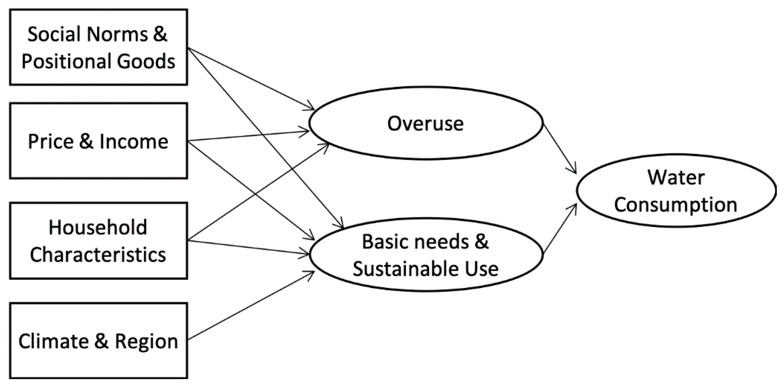
Figure 1 summarizes the schematic diagram of our study. Total water consumption is defined by sustainable uses (including consumption for basic needs) and water overuses. The sustainable use of water may depend primarily on economic factors (price and income) and socioeconomic characteristics. For example, the number and composition of family members may define the volume of water for basic needs. In turn, social norms and positional goods may primarily define the water overuse. Social norms may also exert an influence on the sustainable use when stimulating water-saving habits. Household characteristics, such as large houses, may also be linked to water overuse and are our control variables.

3.2. Endogeneity

We have two potentially endogenous variables in our analysis, $P_i$ and ${\overline{C}}_i$. Average price $P_i$ may be endogenous because SP adopts a block tariff structure, and changes in household consumption ($C_i$) may also change the average price charged per volume of water (reverse causality). Also, the average consumption in the neighborhood ${\overline{C}}_i$ may be endogenous because unobservable factors ($v_i$) affecting $C_i$ (e.g., weather shocks) may also affect demand in the neighborhood (omitted variable bias). We tested the endogeneity of $P_i$ and ${\overline{C}}_i$ using Wooldridge’s score [53] and the C-statistic [54]. The null hypothesis of this statistic is that the variable is exogenous (uncorrelated with errors $v_i$).

We used estimators based on instrumental variables (IVs) to obtain consistent estimators for Equation (1) with endogenous regressors. In the first stage, we estimated the reduced forms of the endogenous variables $P_i$ and ${\overline{C}}_i$ using the following equations:

$$\ln P_i={\theta }_1\ln Y_i+{\mathrm{x}}_i^{\prime }\mathsf{\beta }+{\mathrm{z}}_i^{\prime }{\mathsf{\pi }}_1+{\epsilon }_i$$

(2)

$$\ln {\overline{C}}_i={\theta }_2\ln Y_i+{\mathrm{x}}_i^{\prime }\mathsf{\beta }+{\mathrm{z}}_i^{\prime }{\mathsf{\pi }}_2+u_i$$

(3)

Vector ${\mathrm{z}}_i^{\prime }$ contains two IVs for $P_i$, and two for ${\overline{C}}_i$ (Table 1). The IVs for $P_i$ are the average energy cost in the neighborhood and the average gas price in the neighborhood. Energy and gas costs are expected to be related to the average water price ($P_i$) since water, energy, and gas are primarily provided by Brazil’s public sector. These services include a common and strong political component in the formation of their final consumer price. The water supply service in Brazil is the responsibility of state and municipal governments. The final consumer price refers to the cost for collection, chemical treatment, water distribution, and sewage, which public sanitation agencies control. The price of gas is defined by the Brazilian state oil company (Petrobras), and the federal government has a strong influence on the final retail price. According to Petrobras [55], 53% of the final retail gas price is based on public costs: the value charged by Petrobras distribution stations plus federal and state taxes. The remaining 47% is defined by distribution services, which private companies control. In energy, the average price includes three major components: (i) generation, (ii) transmission and distribution, and (iii) sector taxation and charges. Federal laws define sector taxes and charges, and some are levied on distribution costs, while others are related to generation and transmission costs [56]. Municipal governments may also tax companies that supply water, energy, and gas, influencing the final price.

The instruments for ${\overline{C}}_i$ are the average number of household members and the average number of fans per household in the census tract. We selected these IVs based on a strategy similar to that proposed by Kelejian and Robinson [57] and Kelejian and Prucha [58], using a spatial lag of regressors with the most significant relationships with the dependent variable. In our case, the average numbers of household members and fans in the household are the independent variables with one of the most considerable explanatory powers in the water demand function (vector x in Equation (1)). The average number of household members in the census tract is a proxy for human consumption. The average number of fans is a proxy for the neighborhood’s climate conditions, which also affect water demand.

IVs must satisfy two basic requirements: be strongly correlated with the endogenous variables ($P_i$ and ${\overline{C}}_i$) and be uncorrelated with the unobserved errors ($v_i$). The former condition can be tested by the IVs’ marginal contribution (relevance) in the first stage regressions (Equations (2) and (3)). We used the Wald F-statistic to test the null hypothesis that the instruments are not correlated with the endogenous regressors [54]. In turn, we used the Sargan-Hansen test [54] to check the second assumption (exogeneity of our IVs). This test’s null hypothesis is that the variables are valid instruments, i.e., uncorrelated with the errors $v_i$.

In the second stage, we used different methods to estimate the structural form (Equation (1)): (i) the traditional two-stage least squares (2SLS); (ii) the limited information maximum likelihood (LIML) [59]; (iii) the generalized method of moments (GMM) [60]; and (iv) the control function (CF) [61]. The idea of this comparison is to check the robustness of our estimates under different assumptions. The 2SLS estimators are asymptotically valid when we have good instruments (exogenous and strongly correlated with the endogenous variables). The LIML method is less efficient than the 2SLS but more robust in small samples and overidentification restrictions [62]. Baltagi [63] also highlights that the LIML estimators are consistent even when we have weak instruments. The GMM estimators are consistent and more robust to functional specification problems than the LIML estimators [64]. However, the GMM estimators’ efficiency depends on the assumption of homoscedasticity and independent errors [65]. The GMM estimators may also be inefficient in small samples [66]. Finally, the CF controls for endogeneity by introducing the reduced form’s residuals (${\epsilon }_i$ and $u_i$) in Equation (1), which are proxies for the unobservable factors related to the endogenous variables $P_i$ and ${\overline{C}}_i$ [61]. The CF method provides consistent estimates and an easy alternative to test the endogeneity of $P_i$ and ${\overline{C}}_i$: the t-statistic for coefficients associated with the residuals ${\epsilon }_i$ and $u_i$ introduced in Equation (1) [67].

3.3. Sample Selectivity

Another important source of bias in the estimation of Equation (1) refers to the sample selectivity. Families may not report water consumption ($C_i=0)$ for reasons other than those predicted by Equation (1), such as refusal to provide information or the respondent’s lack of knowledge about water consumption. The latter situation is common in households without water metering. Many buildings and informal settlements in Brazil share the cost of water provision service among residents. According to data from POF 2008/2009, 50% of SP households did not report their water consumption. If this non-reporting is not a random phenomenon in our population, the estimates obtained from the strategies described previously can be biased and inconsistent [68].

We used Heckman’s method [69] to control potential sources of selectivity bias in our data. This strategy considers that two separate equations define water demand: the probability of positive water consumption ($C_i>0$) (Equation (4)) and the water demand function for positive values of consumption (Equation (5)). Specifically:

$$\mathrm{Pr}\left(D_i=1\right)=\mathsf{\Phi }\left({\mathrm{w}}_i^{\prime }\mathsf{\gamma }\right)$$

(4)

$$\mathrm{E}\left[\ln C_i|D_i=1\right]=\alpha +{\theta }_1\ln P_i+{\theta }_2\ln Y_i+\delta \ln {\overline{C}}_i+{\mathrm{x}}_i^{\prime }\mathsf{\beta }+\rho \lambda \left({\mathrm{w}}_i^{\prime }\mathsf{\gamma }\right)$$

(5)

where $D_i$ is a binary variable that assumes 1 if family $i$ reports water consumption ($C_i>0$), and assumes 0 otherwise. The nonlinear function $\mathsf{\Phi }$, usually represented by a probit function, defines the household’s probability of reporting water consumption (selection equation). The vector ${\mathrm{w}}_i^{\prime }$ contains the determinants of the selection equation, and $\mathsf{\gamma }$ is the respective vector of coefficients. The term $\lambda \left({\mathrm{w}}_i^{\prime }\mathsf{\gamma }\right)$ in Equation (5), called the inverse Mills ratio (IMR), controls for selectivity bias in the water demand function. If $\rho =0$, then the correction of selectivity is unnecessary, and the estimators of Equation (1) are consistent; if $\rho \ne 0$, then the estimators of Equation (5) are the only consistent estimators.

Ideally, the determinants of the selection equation (${\mathrm{w}}_i^{\prime }$) contain all regressors presented in Equation (1) plus at least one IV [70]. The IVs incorporated in our selection equation refer to other public services (Table 1): binaries for access to garbage collection and living on a paved street. According to Basani et al. [71], these variables define the likelihood of living in a place with access to the public water system and, consequently, the existence of water metering (i.e., whether the household is charged individually or collectively). In this respect, we expect that these variables may determine the probability of a household reporting its water consumption ($D=1$), but have no direct impact on the volume of water consumed $C$.

Finally, we used the strategy proposed by Wooldridge [72] to control for endogeneity (Equations (2) and (3)) and selectivity (Equations (4) and (5)) simultaneously. In the first stage, we estimate the IMR by fitting the selection Equation (4). In the second stage, we use the methods 2SLS, LIML, GMM, and CF to estimate the water demand conditioned on $D_i=1$ and control for the IMR [72] In the second stage, we included the IMR estimate both in the reduced Equations (2) and (3) and in the structural Equation (1). This strategy obtains consistent estimators in the presence of endogeneity and selectivity. We also used the White covariance matrix to obtain robust estimators for the standard errors [65].

3.4. Quantile Regression

The previous methods estimate the peer effect on average water consumption. However, the impacts may differ along with the water consumption distribution, i.e., the peer effect may differ among water consumption classes. We used a quantile regression [73] to evaluate how peer effects impact water consumption quantiles. Another main advantage of quantile regression is the robustness to outliers [74]. The conditional quantile regression for the $\tau \mathrm{th}$ quantile with control for selectivity is given by

$$Q_{\tau }\left(\ln C_i{|\mathrm{x}}_i,D_i=1\right)={\alpha }_{\tau }+{\theta }_{1\tau }\ln P_i+{\theta }_{2\tau }\ln Y_i+{\delta }_{\tau }\ln {\overline{C}}_i+{\mathrm{x}}_i^{\prime }{\mathsf{\beta }}_{\tau }+Q_{\tau }\left[\rho \lambda \left({\mathrm{w}}_i^{\prime }\mathsf{\gamma }\right)\right]$$

(6)

We simultaneously controlled for selectivity and endogeneity using a two-stage strategy proposed by Wooldridge [72]: (i) we used the method proposed by Buchinsky [75,76] to estimate a polynomial function $Q_{\tau }$ of the IMR, $\lambda \left({\mathrm{w}}_i^{\prime }\mathsf{\gamma }\right)$, and (ii) we controlled for the endogeneity of $P$ using the method proposed by Dufrenot et al. [77]. To simplify our analyses, we did not control for the endogeneity of ${\overline{C}}_i$ because our estimates (shown below) suggested that this variable is exogenous.

4. Results

4.1. The Impacts on Average Water Consumption

We estimated Equation (1) for the average water consumption using 2SLS, LIML, GMM, CF, and OLS (ordinary least square) estimators (

Table 2. Fixed effect estimates of the models for the dependent variable log of household water consumption (robust standard error estimates between parentheses). State of São Paulo, Brazil.

Independents Variables	Dependent Variable: Ln Residential Water Consumption
	OLS			Instrumental Variable Models, with Sample Selection Control
	[1]	[2]	[3]	2SLS	LIML	GMM	CF Ø
Ln Average water price	−0.620 ***	−0.628 ***	−0.640 ***	−0.349 ***	−0.348 ***	−0.351 ***	−0.336 ***
	(0.032)	(0.029)	(0.028)	(0.103)	(0.104)	(0.103)	(0.093)
Ln Total household income	0.214 ***	0.129 ***	0.110 **	0.085 **	0.085 **	0.086 **	0.083 **
	(0.021)	(0.026)	(0.027)	(0.028)	(0.028)	(0.028)	(0.028)
Ln Average water consumption in the neighborhood	0.280 ***	0.230 ***	0.205 ***	0.207 *	0.207 *	0.204 *	0.202 **
	(0.032)	(0.031)	(0.031)	(0.097)	(0.098)	(0.097)	(0.070)
Mills ratio				0.220	0.220	0.252	0.252
				(0.238)	(0.238)	(0.221)	(0.255)
Residuals reduced form for Ln Average water price							−0.322 **
							(0.095)
Reduced form residuals for Ln Average water consumption in the neighborhood							−0.005
							(0.076)
Control variables for household and family structure, and imputed rent	No	Yes	Yes	Yes	Yes	Yes	Yes
Control variables for home appliances, household location and proxies for weather conditions	No	No	Yes	Yes	Yes	Yes	Yes
Observations	1806	1806	1805	1799	1799	1799	1799
R2	0.453	0.510	0.527	0.468	0.467	0.468	0.531

* p < 0.05; ** p < 0.01; *** p < 0.001. ^Ø Model estimated by the OLS method. Ordinary least squares (OLS); two-stage least squares (2SLS); limited information maximum likelihood (LIML); generalized method of moments (GMM); control function (CF).

).

Table A2. First-stage estimates for the dependent variables log average water price and water consumption in the neighborhood.

Independents Variables	First Stage
	Selection Model	Instrumental Variable Model
		Ln Average Water Price	Ln Water Consumption in the Neighborhood
Ln Total household income	0.005	0.074 *	−0.098 ***
	(0.051)	(0.032)	(0.026)
Formal roof	0.671 ***	0.126	−0.280 ***
	(0.073)	(0.102)	(0.057)
Concrete walls	0.100	−0.128	−0.224
	(0.181)	(0.117)	(0.130)
Floor is ceramic, flagstone, stone, or cement	0.273 **	0.009	0.003
	(0.103)	(0.081)	(0.053)
Rooms used as dormitory	0.152 ***	−0.047	0.043 *
	(0.043)	(0.034)	(0.021)
Sewage hookup	0.303 ***	0.106	−0.093
	(0.091)	(0.066)	(0.047)
Reference person is a woman	−0.166 **	0.052	−0.034
	(0.063)	(0.043)	(0.031)
Age of the reference person	0.007 *	0.002	−0.002
	(0.003)	(0.002)	(0.001)
Years of education of the reference person	−0.006	−0.000	−0.001
	(0.004)	(0.002)	(0.002)
Number of children in the household	−0.034	−0.016	−0.018
	(0.033)	(0.022)	(0.016)
Number of seniors in the household	−0.116	−0.005	−0.000
	(0.064)	(0.035)	(0.028)
Estimated household rent	−0.035	0.013	0.010
	(0.065)	(0.040)	(0.028)
Freezer	0.075	−0.079	0.016
	(0.091)	(0.054)	(0.046)
Fridge	0.056	−0.017	−0.149
	(0.208)	(0.171)	(0.105)
Dishwasher	−0.042	0.217**	0.049
	(0.149)	(0.078)	(0.070)
Washing machine	0.058	−0.045	0.066 *
	(0.065)	(0.037)	(0.029)
Clothes dryer	−0.311 *	−0.056	−0.079
	(0.132)	(0.087)	(0.061)
Iron	0.312 **	−0.139	−0.047
	(0.107)	(0.078)	(0.054)
Household is located in the state capital	−0.045	−0.049	0.170 ***
	(0.085)	(0.058)	(0.046)
Household is located in the metropolitan region	−0.044	0.058	−0.166 ***
	(0.089)	(0.050)	(0.039)
Household is located in a rural area	−0.434 ***	0.229 *	−0.166 *
	(0.098)	(0.094)	(0.070)
Number of air conditioners	−0.095	0.139 ***	−0.008
	(0.086)	(0.042)	(0.033)
Number of fans	0.041	−0.043 *	0.026
	(0.030)	(0.020)	(0.014)
Number of electric showers	0.073	0.021	−0.017
	(0.053)	(0.030)	(0.021)
Garbage collection	0.833 ***
	(0.172)
Paved street	0.418 ***
	(0.101)
Ln Average energy cost in the neighborhood	−0.115	0.307 ***	0.383 ***
	(0.069)	(0.068)	(0.043)
Ln Average gas price in the neighborhood	0.980 **	1.456 ***	−1.120 ***
	(0.338)	(0.301)	(0.217)
Residents in the neighborhood	0.074	−0.071*	0.146 ***
	(0.049)	(0.036)	(0.027)
Fans in the neighborhood	−0.030	−0.139 ***	0.132 ***
	(0.047)	(0.037)	(0.032)
Mills ratio		−0.244	−0.072
		(0.207)	(0.103)
Constant	−3.357 ***	−0.848	1.942 ***
	(0.633)	(0.638)	(0.433)
Observations	3409	1806	2929
Pseudo-R-squared	0.1536	0.131	0.214

* p < 0.05; ** p < 0.01; *** p < 0.001.

in Appendix A shows the estimates for the selection equation and the first stage of the instrumental variables. The idea of using OLS estimators is to check to what extent these traditional estimates may be biased due to endogeneity and selectivity. The models estimated by OLS combine different groups of control variables to evaluate how the estimate of the peer effect may be biased due to omitted variables. Model 1 (benchmarking) represents Equation (1) without control variables (vector x). Model 2 adds controls for family and household characteristics and rent, while model 3 adds controls for home appliances, location, and proxies for climatic conditions. The idea is to evaluate how the total peer effect in model 1 may be explained by personal or household characteristics controlled in models 2 and 3. The estimates for the methods 2SLS, LIML, GMM, and CF include all control variables (model 3). All models present suitable goodness-of-fit statistics, with $R^2$ ranging from 45% (OLS model 1) to 53% (OLS model 3).

The estimates of the peer effect ($\delta$) corroborate the hypothesis that comparisons with neighbors influence household water consumption. The OLS estimates range from $0.280$ (model 1) to $0.205$ (model 3), while the 2SLS, GMM, LILM, and CF estimates range from $0.202$ to $0.207$. Specifically, residential water consumption tends to increase by nearly $0.20\%$ for each $1\%$ increase in the neighborhood’s consumption. The small differences between the estimates of models 1, 2, and 3 suggest that a small share of the total peer effect (model 1) can be attributed to similar households in the same neighborhood. Moreover, the small differences between the estimates obtained by OLS and IV methods also suggest that the estimates are robust against selectivity and endogeneity.

The estimates for income elasticity (${\theta }_2$) and price elasticity (${\theta }_1$) corroborate the assumption that water is a normal and necessary good, showing positive income elasticity of demand and low price and income elasticities. The estimates for income elasticity are more sensitive to changes in the model specifications (models 1–3) than those for price elasticity. In general, the larger the number of control variables, the lower the estimate for income elasticity ($0.214$ in model 1, $0.129$ in model 2, and $0.110$ in model 3). This difference is because income tends to be strongly correlated with household and family characteristics controlled in models 2 and 3. In turn, the estimates for both income and price elasticity considerably decrease once we control for endogeneity and selectivity (2SLS, LIML, GMM, and CF). For example, the price elasticity shifted from $-0.640$ in model 3 to $-0.336$ in the CF method, and the income elasticity shifted from $0.110$ in model 3 to $0.083$ in the CF method.

4.2. The Consistency of the Estimates

Our results indicate that selectivity is not a central concern. All the estimates for the IMR are insignificant at 5%, suggesting that water consumption is not strongly affected by unobserved factors that determine the likelihood of reporting positive consumption (e.g., water metering in the household). Even with insignificant estimates for the IMR, the IV estimators remain consistent, although they lose efficiency [70,72].

In turn, we have evidence that $P$ is endogenous, while $\overline{C}$ is exogenous. First, the endogeneity tests based on Wooldridge’s score, robust regression, and C-statistic are significant at 1%, suggesting that at least one variable ($P_i$ or ${\overline{C}}_i$) is endogenous, i.e., related to the errors $v_i$ in Equation (1) (Appendix A—

Table A1. Test for instrumental variable models.

	Instrumental Variable Models, with Sample Selection Control
	2SLS	LIML	GMM
Endogeneity Test: Ho: variables are exogenous
Wooldridge’s score	12.527 **
Robust regression	5.705 **
C Statistic		11.147 **	11.275 **
Overidentification Test:
Basman	0.516
Wooldridge’s robust score	0.508
Sargan–Hansen score	0.454	0.314	0.315
Weak instrument test: First-stage regression robust F
Ln Average water price	11.798 ***	11.798 ***	11.798 ***
Ln Average water consumption in the neighborhood	23.598 ***	23.598 ***	23.598 ***

** p < 0.01; *** p < 0.001.

). The estimates obtained by the CF method indicate that only the residuals ${\widehat{\epsilon }}_i$ are significant in Equation (1), suggesting that only the variable $P_i$ is endogenous. Previous studies have also confirmed the endogeneity of price in the water demand [34,37]. The residuals ${\widehat{u}}_i$ are not significant in the water demand, suggesting that ${\overline{C}}_i$ is exogenous. In other words, we do not have unobservable factors that may simultaneously affect household water consumption and consumption in the neighborhood.

The overidentification and weak instrument tests indicate that the IVs are exogenous and strongly correlated to the endogenous variables, i.e., we have valid instruments (Appendix A—Table A1). The Sargan-Hansen test is insignificant at 5%, suggesting that the instruments are exogenous, i.e., uncorrelated to the errors $v_i$ in Equation (1). The weak instrument tests indicate that the instruments for $P_i$ and ${\overline{C}}_i$ are strongly related to these endogenous variables ($F>10$) and significant at $0.1\%$.

4.3. Impacts on Water Consumption Quantiles

We used Equation (5) to estimate the conditional quantile regressions for quantiles 10, 25, 50, 75, and 90 (

Table 3. Determinants of household water consumption: quantile regression. State of São Paulo, Brazil. Standard deviation between parentheses.

Independents Variables	Dependent Variable: Ln Residential Water Consumption
	Two-Stage Quantile Approach
	Q 10	Q 25	Q 50	Q 75	Q 90
Ln Average water price	−0.004	−0.034	−0.371 *	−0.786 ***	−0.568 **
	(0.250)	(0.169)	(0.173)	(0.170)	(0.201)
Ln Total household income	0.065	0.070	0.116 ***	0.114 ***	0.172 ***
	(0.045)	(0.037)	(0.030)	(0.023)	(0.048)
Ln Average water consumption in the neighborhood	0.204	0.182 *	0.235 **	0.335 ***	0.488 ***
	(0.108)	(0.073)	(0.077)	(0.076)	(0.090)
Mills ratio	−0.886	−0.374	0.114	1.382	2.323
	(2.407)	(0.966)	(1.665)	(1.557)	(4.052)
Mills ratio2	1.079	0.410	−0.369	−0.725	−2.717
	(6.464)	(2.247)	(4.738)	(4.793)	(13.436)
Control variables for household and family structure	Yes	Yes	Yes	Yes	Yes
Control variables for home appliances, household location and proxies for weather conditions	Yes	Yes	Yes	Yes	Yes
Observations	1799	1799	1799	1799	1799
Pseudo-R2	0.083	0.081	0.120	0.166	0.250

* p < 0.05; ** p < 0.01; *** p < 0.001.

). Based on our prior results (Table 2), we assumed the endogeneity of $P_i$ and the exogeneity of ${\overline{C}}_i$. We controlled for selectivity using a quadratic polynomial function for the IMR [75,76]. The estimates for both linear and quadratic IMR are insignificant at 5%, suggesting that selectivity is not a central concern in the quantile water functions. The models better fitted at the highest quantiles—the pseudo-$R^2$ ranges from 8.3% (10th quantile) to 25% (90th quantile), suggesting that the peer effect and socioeconomic characteristics best explain the largest consumption levels. The pseudo-$R^2$ measures the differences between the estimated and raw quantiles and its interpretation is analogous to the conventional $R^2$ of least-squares regression [78].

The peer effect estimates are positive and significant in most quantiles, except for the 10th quantile. The magnitude of the peer effect increases for the highest water consumption quantiles. The largest impact is observed in the 90th quantile: household water consumption increases by 0.49% for each 1% increase in neighborhood consumption.

Our estimates also suggest that the price and income elasticities are most relevant for the largest water consumption levels (within the same classes of family and household characteristics). The price elasticities are only significant between the 50th and the 90th quantiles, ranging from $-0.371$ (50th quantile) to $-0.568$ (90th quantile). The income elasticities are significant at the upper quantiles, but the highest estimate is observed in the 90th quantile (0.172).

5. Discussion

Our results highlight that the absolute consumption hypothesis does not solely drive water demand. Relative consumption patterns also play a significant role in water demand, especially among those overconsuming water. Peer behavior has already been proven to be an essential source of information regarding the costs and benefits of different consumption choices [47]. However, few studies have analyzed the role of peer effects on essential environmental goods or services.

The peer effects on water consumption would reflect social norms, which are the beliefs of individuals about what others do or approve of doing, and about what is considered normal, expected, or desirable behavior in a social group [44,79]. Social norms can potentially influence demand decisions when generating regularities in individuals’ consumption behavior. Social norms can also represent a code identifying social relations, allowing the classification of individuals into a social group [80]. In water consumption, social norms may refer to the way people use and save water for daily indoor and outdoor activities, such as washing, cleaning, and using water-saving household items.

On the other hand, household water demand would be related to the consumption and maintenance of positional goods [30,81]. The consumption of positional goods reflects social prestige rather than the satisfaction of basic needs. In this sense, the reference group’s consumption is associated with prestige, social normativity, power relations, and symbolic expressions and determines individual consumption preferences. In the case of water consumption, this relationship could be explained, for example, by large homes, gardens, and swimming pools, which may require periodic maintenance and great water demand.

The results also highlight that the peer effect differs largely between the conditional quantiles. The peer effect is insignificant in the 10th quantile, where water consumption likely meets basic needs for the respective social group. The peer effect becomes significant at the 25th quantile and increases for the groups with the highest consumption levels. The influence of social norms and the consumption of positional goods increase once social groups meet their basic needs [30]. According to Hirsch [29], consumption increasingly depends on peer effects as demand increases and acquires an increasingly social dimension. Once basic needs are met, people would begin to redefine their consumption preferences incorporating positional goods and services, such as large swimming pools and green gardens, which would increase residential water consumption [30,36].

The estimates for price and income elasticities are also following those obtained in prior studies, reinforcing the idea that water demand is inelastic to price and income. Our estimates for price elasticity (nearly $-0.35$) are very similar to those obtained in the following: Agthe and Billings [82], $\left[-0.50,-0.37\right]$; Chicoine et al. [83], $\left[-0.42,-0.22\right]$; Williams and Suh [84], $\left[-0.48,-0.25\right]$; Nieswiadomy and Molina [85], $\left[-0.55,-0.36\right]$; Pint [86] $\left[-0.47,-0.20\right]$; Nauges and Thomas [87], $\left[-0.40\right]$; and Gaudin [88], $\left[-0.37\right]$. Meanwhile, our estimates for income elasticity (nearly $0.09$) are similar to those of the following: Chicoine et al. [83], $\left[0.01,0.14\right]$; Moncur [89], $\left[0.04,0.08\right]$; Barkatullah and Nadira [90], $\left[0.07\right]$; Höglund [91], $\left[0.07,0.13\right]$; Garcia and Reynaud [92], $\left[0.03\right]$; and Martínez-Espiñeira and Nauges [93], $\left[0.07,0.13\right]$. The small price and income elasticities reflect that water is an essential good for most households, i.e., these households will continue consuming water regardless of price or income changes.

Price and income elasticity also differ considerably along with the conditional quantile functions. Price elasticity is insignificant at lower quantiles and increases at the upper quantiles of water consumption, reaching $-0.488$ in the 90th quantile. We found similar results for income elasticity. The impacts of income changes on water demand are insignificant at lower consumption quantiles, and they increase near the 75th and 90th quantiles; this is probably associated with a great demand for water for the maintenance of positional goods.

These results reflect that water is an essential good and that water has zero substitutability at levels close to those for meeting basic needs [94]. In other words, households consuming shallow water volumes probably ensure a minimum supply of water for basic needs. Once water consumption increases, households become more sensitive to price and income changes. Therefore, price and income elasticities increase as consumption meets basic needs.

Finally, our results show the price–water consumption elasticity in the 75th quantile is greater than that in the 90th quantile. This result suggests that price-oriented policies may not necessarily reduce the water consumption of households having the highest consumption levels. Probably, households overconsuming water may have socioeconomic conditions to mitigate the impact of price changes. These results reinforce the evidence that price-based policies may depend on the type of household and may primarily affect lower-income households [36].

6. Conclusions

We analyze the peer effect on residential water consumption, providing theoretical and empirical contributions. Our main theoretical contribution is to highlight that social behavior is relevant to explain water consumption. Among households with similar characteristics, the higher the water consumption, the larger the peer effect. In other words, overconsumption of water seems to be influenced mainly by the behavior of social peers. Our main empirical contribution is to apply a strategy to analyze water consumption functions at different consumption levels that simultaneously control endogeneity and selectivity.

Our results highlight the importance of a reference social group for water consumption decisions. Social norms may interfere in household habits and patterns of water consumption, acting as a way of identifying and establishing a hierarchy of individuals within the reference social group. Water consumption may also be related to the ownership and maintenance of positional goods, such as large homes, gardens, and swimming pools. However, we believe that social norms may better explain the peer effect. Our estimates for the peer effect barely changed once we introduced several controls for family and household characteristics, including imputed rent.

We applied an innovative methodological approach, combining quantile regression with estimation strategies that simultaneously control sample selectivity and endogeneity. We did not find significant evidence of sample selectivity, which would imply that households not reporting water consumption are merely random events in the water demand function. We also did not find evidence of endogeneity in the neighborhood’s average water consumption, suggesting that our models somewhat control for unobservables that would affect both household and neighborhood water demand (e.g., weather shocks). However, we found strong evidence of endogeneity in the average price, implying that random shocks in water demand also impact the average water price. This result was expected, as block tariffs define the water price in SP. Nonetheless, the most important result is that our estimates for peer effects are robust throughout the different empirical strategies.

The estimates for price and income elasticity are also consistent with those obtained in previous studies. In particular, we found that water consumption is inelastic to price and income since water is an essential good and presents zero substitutability, although price and income elasticity increase along with the conditional quantile functions. Once basic needs are met, water demand may become increasingly driven by relative consumption and become more sensitive to changes in price and income.

One limitation of this study is that the neighborhood is based on the census tracks rather than on contiguity or geographic distance criteria. For example, a contiguity criterium would consider households sharing common boundary lines. Future research studies would also investigate how weather shocks may affect the estimates of peer effects on water consumption. Regional and some household characteristics may be good proxies for climate differences but may be limited in the ability to control, for example, extreme climate events in one specific locality. Despite some limitations, our study reinforces the importance of peer effects found in socioeconomic literature and provides novel elements to guide policies on residential water consumption. We present essential findings to guide the policies of sustainable water use in urban areas. In particular, our results suggest that policies oriented toward changing social habits of water consumption may be as effective as price-oriented policies at curbing excessive water consumption. These policies may include, for example, public campaigns to change the widespread habit in Brazil of washing sidewalks and cars in the streets with abusive quantities of water. Such policies could result in lower relative welfare losses compared to traditional price-based policies.

Policies based on behavioral economics can be implemented to induce the sustainable use of water resources. For example, nudges might provide information on saving habits in the neighborhood and stimulate other households to save water. Our results indicate that those households overconsuming water are precisely those more likely to change their habits based on the peer’s influence.

References

- WHO. Domestic Water Quantity, Service Level and Health; World Health Organ: Geneva, Switzerland, 2003. [Google Scholar]
- Dziegielewski, B. Management of water demand: Unresolved issues. J. Contemp. Water Res. Educ. 2011, 114. [Google Scholar]
- Wang, X.-J.; Zhang, J.-Y.; Gao, J.; Shahid, S.; Xia, X.-H.; Geng, Z.; Tang, L. The new concept of water resources management in China: Ensuring water security in changing environment. Environ. Dev. Sustain. 2018, 20, 897–909. [Google Scholar] [CrossRef]
- Turral, H.; Burke, J.; Faurés, J.-M. Climate Change, Water and Food Security; FAO: Rome, Italy, 2011. [Google Scholar]
- Maccheroni, F.; Marinacci, M.; Rustichini, A. Social decision theory: Choosing within and between groups. Rev. Econ. Stud. 2012, 79, 1591–1636. [Google Scholar] [CrossRef]
- Fortin, B.; Yazbeck, M. Peer effects, fast food consumption and adolescent weight gain. J. Health Econ. 2015, 42, 125–138. [Google Scholar] [CrossRef] [PubMed] [Green Version]
- Schelling, T.C. Dynamic models of segregation. J. Math. Sociol. 1971, 1, 143–186. [Google Scholar] [CrossRef]
- Schelling, T.C. A Process of Residential Segregation: Neighborhood Tipping; Pascal, A., Ed.; Lexington Books: Lanham, MA, USA, 1972. [Google Scholar]
- Benhabib, J.; Bisin, A.; Jackson, M.O. Handbook of Social Economics; Elsevier: Amsterdam, The Netherlands, 2011; ISBN 9780444531872. [Google Scholar]
- Rayo, L.; Becker, G.S. Habits, peers, and happiness: An evolutionary perspective. Am. Econ. Rev. 2007, 97, 487–491. [Google Scholar] [CrossRef]
- House-Peters, L.; Pratt, B.; Chang, H. Effects of urban spatial structure, sociodemographics, and climate on residential water consumption in Hillsboro, Oregon. JAWRA J. Am. Water Resour. Assoc. 2010, 46, 461–472. [Google Scholar] [CrossRef]
- Côrtes, P.L.; Torrente, M.; Pinto, A.P.A.; Ruiz, M.S.; Dias, A.J.G.; Rodrigues, R. Crise de abastecimento de água em São Paulo e falta de planejamento estratégico. Estud. Av. 2015, 29, 7–26. [Google Scholar] [CrossRef] [Green Version]
- Hardin, G. The tragedy of the commons. The population problem has no technical solution; It requires a fundamental extension in morality. Science 1968, 162, 1243–1248. [Google Scholar] [CrossRef] [Green Version]
- Hastie, R.; Dawes, R.M. Rational Choice in an Uncertain World: The Psychology of Judgment and Decision Making; SAGE: Newbury Park, CA, USA, 2010; ISBN 1412959039. [Google Scholar]
- Drakopoulos, S. The History of the Mainstream Rejection of Interdependent Preferences; Technical Report No. 26769; MPRA Pap.: Munich, Germany, 2010. [Google Scholar]
- Frank, R.H. Luxury Fever: Money and Happiness in an Era of Excess; Princeton University Press: Princeton, NJ, USA, 2000; ISBN 0691070113. [Google Scholar]
- Frank, R.H. Does context matter more for some goods than others? In The Evolution of Consumption: Theories and Practices; Bianchi, M., Ed.; Emerald Group Publishing Limited: Bingley, UK, 2007; pp. 231–248. [Google Scholar]
- Levine, A.S.; Frank, R.H.; Dijk, O. Expenditure cascades. SSRN Electron. J. 2010. [Google Scholar] [CrossRef] [Green Version]
- Alpizar, F.; Carlsson, F.; Johansson-Stenman, O. How much do we care about absolute versus relative income and consumption? J. Econ. Behav. Organ. 2005, 56, 405–421. [Google Scholar] [CrossRef] [Green Version]
- Carlsson, F.; Gupta, G.; Johansson-Stenman, O. Choosing from behind a veil of ignorance in India. Appl. Econ. Lett. 2003, 10, 825–827. [Google Scholar] [CrossRef] [Green Version]
- Carlsson, F.; Daruvala, D.; Johansson-Stenman, O. Are people inequality-averse, or just risk-averse? Economica 2005, 72, 375–396. [Google Scholar] [CrossRef] [Green Version]
- Heffetz, O.; Frank, R.H. Preferences for status: Evidence and economic implications. In Handbook of Social Economic; Elsevier: Amsterdam, The Netherlands, 2008. [Google Scholar]
- Carlsson, F.; Johansson-Stenman, O.; Martinsson, P. Do you enjoy having more than others? Survey evidence of positional goods. Economica 2007, 74, 586–598. [Google Scholar] [CrossRef] [Green Version]
- Tobias, K.; Tobias, L. Relative Consumption Preferences and Public Provision of Private Goods; Technical Report No: SP II 2016-213; Wissenschaftszentrum Berlin für Sozialforschung: Berlin, Germany, 2016. [Google Scholar]
- Samuelson, L. Information-based relative consumption effects. Econometrica 2004, 72, 93–118. [Google Scholar] [CrossRef]
- Frank, R.H. Choosing the Right Pond: Human Behavior and the Quest for Status; Oxford University Press: Oxford, UK, 1985; ISBN 0195035208. [Google Scholar]
- Bonan, J.; Battiston, P.; Bleck, J.; LeMay-Boucher, P.; Pareglio, S.; Sarr, B.; Tavoni, M. Social Interaction and Technology Adoption: Experimental Evidence from Improved Cookstoves in Mali; Technical Report No: 047.2017; Fondazione Eni Enrico Mattei: Milan, Italy, 2017. [Google Scholar]
- Veblen, T. The Theory of the Leisure Class: An Economic Study of Institutions; Modern Library: New York, NY, USA, 1934. [Google Scholar]
- Hirsch, F. Social Limits to Growth; Routledge: Milton, UK, 1995; ISBN 0415119588. [Google Scholar]
- Domene, E. Changing patters of water consumption in the suburban Barcelona: Lifestiles and welfare as explanatory factors. Investig. Geogr. 2014. [Google Scholar] [CrossRef] [Green Version]
- Andrade, T.; Brandão, A.; Lobão, W.; da Silva, S. Saneamento urbano: A demanda residencial por água. Pesqui. Planej. Econ. 1995, 25, 427–448. [Google Scholar]
- Ito, K. Do consumers respond to marginal or average price? Evidence from nonlinear electricity pricing. Am. Econ. Rev. 2014, 104, 537–563. [Google Scholar] [CrossRef] [Green Version]
- Foster, H.S.; Beattie, B.R. Urban residential demand for water in the United States. Land Econ. 1979, 55, 43. [Google Scholar] [CrossRef]
- Arbués, F.; García, M.Á.; Martínez, R. Estimation of residential water demand: A state-of-the-art review. J. Socio Econ. 2003, 32, 81–102. [Google Scholar] [CrossRef]
- Sebri, M. A meta-analysis of residential water demand studies. Environ. Dev. Sustain. 2014, 16, 499–520. [Google Scholar] [CrossRef]
- Deyà-Tortella, B.; Garcia, C.; Nilsson, W.; Tirado, D. Analysis of water tariff reform on water consumption in different housing typologies in Calvià (Mallorca). Water 2017, 9, 425. [Google Scholar] [CrossRef] [Green Version]
- Worthington, A.C.; Hoffman, M. An empirical survey of residential water demand modelling. J. Econ. Surv. 2008, 22, 842–871. [Google Scholar] [CrossRef] [Green Version]
- Ferraro, P.J.; Price, M.K. Using nonpecuniary strategies to influence behavior: Evidence from a large-scale field experiment. Rev. Econ. Stat. 2013, 95, 64–73. [Google Scholar] [CrossRef]
- Datta, S.; Miranda Montero, J.J.; Zoratto, L.D.C.; Calvo-Gonzalez, O.; Darlingm, M.; Lorenzana, K.J.O. A Behavioral Approach to Water Conservation: Evidence from Costa Rica; Technical Report No: 7283; World Bank: Washington, DC, USA, 2015; pp. 1–29. [Google Scholar]
- Peschiera, G.; Taylor, J.E.; Siegel, J.A. Response-relapse patterns of building occupant electricity consumption following exposure to personal, contextualized and occupant peer network utilization data. Energy Build. 2010, 42, 1329–1336. [Google Scholar] [CrossRef]
- Brent, D.; Lott, C.; Taylor, M.; Cook, J.; Rollins, K.; Stoddard, S. Are Behavioral Nudges Moral Taxes? Evidence from a Field Experiment on Water Conservation; University of Chicago: Chicago, IL, USA, 2017. [Google Scholar]
- Seyranian, V.; Sinatra, G.M.; Polikoff, M.S. Comparing communication strategies for reducing residential water consumption. J. Environ. Psychol. 2015, 41, 81–90. [Google Scholar] [CrossRef]
- Peschiera, G.; Taylor, J.E. The impact of peer network position on electricity consumption in building occupant networks utilizing energy feedback systems. Energy Build. 2012, 49, 584–590. [Google Scholar] [CrossRef]
- Schultz, P.W.; Messina, A.; Tronu, G.; Limas, E.F.; Gupta, R.; Estrada, M. Personalized normative feedback and the moderating role of personal norms. Environ. Behav. 2016, 48, 686–710. [Google Scholar] [CrossRef] [Green Version]
- Schultz, P.W.; Nolan, J.M.; Cialdini, R.B.; Goldstein, N.J.; Griskevicius, V. The constructive, destructive, and reconstructive power of social norms. Psychol. Sci. 2007, 18, 429–434. [Google Scholar] [CrossRef] [PubMed] [Green Version]
- Ayres, I.; Raseman, S.; Shih, A. Evidence from two large field experiments that peer comparison feedback can reduce residential energy usage. J. Law Econ. Organ. 2013, 29, 992–1022. [Google Scholar] [CrossRef]
- Cooter, R.D.; Feldman, M.; Feldman, Y. The misperception of norms: The psychology of bias and the economics of equilibrium. Rev. Law Econ. 2008, 4, 889–911. [Google Scholar] [CrossRef] [Green Version]
- Aitken, C.K.; Mcmahon, T.A.; Wearing, A.J.; Finlayson, B.L. Residential water use: Predicting and reducing consumption. J. Appl. Soc. Psychol. 1994, 24, 136–158. [Google Scholar] [CrossRef]
- Kaaukauskas, A.; Broberg, T.; Jaraite, J. Social comparisons in real time: A field experiment of residential electricity and water use. SSRN Electron. J. 2017. [Google Scholar] [CrossRef] [Green Version]
- Allcott, H.; Rogers, T. The short-run and long-run effects of behavioral interventions: Experimental evidence from energy conservation. Am. Econ. Rev. 2014, 104, 3003–3037. [Google Scholar] [CrossRef] [Green Version]
- IBGE. Pesquisa de Orçamentos Familiares 2009–2010; Despesas, Rendimiento e Condições de Vida; IBGE: Rio de Janeiro, Brazil, 2010.
- Rubin, D.B. Statistical Matching Using File Concatenation With Adjusted Weights and Multiple Imputations. J. Bus. Econ. Stat. 1986, 4, 87–94. [Google Scholar] [CrossRef]
- Wooldridge, J.M. Score diagnostics for linear models estimated by two stage least squares. In Advances in Econometrics and Quantitative Economics: Essays in Honor of Professor C. R. Rao; Maddala, G.S., Phillips, P.C.B., Srinivasan, T.N., Eds.; Blackwell Publishing: Oxford, UK, 1995; pp. 66–87. [Google Scholar]
- Baum, C.F.; Schaffer, M.E.; Stillman, S. Instrumental variables and GMM: Estimation and testing. Stata J. Promot. Commun. Stat. Stata 2003, 3, 1–31. [Google Scholar] [CrossRef] [Green Version]
- Petrobras Composição de Preços do Gás Liquefeito de Petróleo—Petrobras. Available online: http://www.petrobras.com.br/pt/produtos-e-servicos/composicao-de-precos-de-venda-ao-consumidor/gas-liquefeito-de-petroleo-glp/ (accessed on 7 November 2018).
- Aneel Cómo é Composta a Tarifa. Available online: http://www.aneel.gov.br/conteudo-educativo/-/asset_publisher/vE6ahPFxsWHt/content/composicao-da-tarifa/654800?inheritRedirect=false (accessed on 22 April 2021).
- Kelejian, H.H.; Robinson, D.P. Spatial autocorrelation: A new computationally simple test with an application to per capita county police expenditures. Reg. Sci. Urban Econ. 1992, 22, 317–331. [Google Scholar] [CrossRef]
- Kelejian, H.H.; Prucha, I.R. A generalized spatial two-stage least squares procedure for estimating a spatial autoregressive model with autoregressive disturbances. J. Real Estate Financ. Econ. 1998, 17, 99–121. [Google Scholar] [CrossRef]
- Anderson, T.; Rubin, H. Estimation of the parameters of a single equation in a complete system of stochastic equations. Ann. Math. Stat. 1949, 20, 18. [Google Scholar] [CrossRef]
- Hansen, L.P. Large sample properties of generalized method of moments estimators. Econometrica 1982, 50, 1029–1054. [Google Scholar] [CrossRef]
- Wooldridge, J.M. Control function methods in applied econometrics. J. Hum. Resour. 2015, 50, 420–445. [Google Scholar] [CrossRef]
- Davidson, R.; MacKinnon, J.G. Estimation and Inference in Econometrics; Oxford University Press: Oxford, UK, 1993; ISBN 0195060113. [Google Scholar]
- Baltagi, B.H. Econometric Analysis of Panel Data, 3th ed.; John Wiley & Sons: New York, NY, USA, 2008. [Google Scholar]
- Zsohar, P. Short introduction to the generalized method of moments. Hung. Stat. Rev. 2012, 16, 150–170. [Google Scholar]
- Greene, W.H. Econometric Analysis; Prentice Hall: Hoboken, NJ, USA, 2003; ISBN 0130661899. [Google Scholar]
- Andersen, T.G.; Sørensen, B.E. GMM estimation of a stochastic volatility model: A Monte Carlo study. J. Bus. Econ. Stat. 1996, 14, 328–352. [Google Scholar] [CrossRef]
- Cameron, A.C.; Trivedi, P.K. Microeconometrics: Methods and Applications; Cambridge University Press: Cambridge, UK, 2005; Volume 53, ISBN 9780521848053. [Google Scholar]
- Aigner, D.J.; Ghali, K. Self-selection in the residential electricity time-of-use pricing experiments. J. Appl. Econom. 1989, 4, 131–144. [Google Scholar] [CrossRef]
- Heckaman, J.T. Sample selection bias as a specification error. Econometrica 1979, 47, 153–161. [Google Scholar] [CrossRef]
- Wooldridge, J.M. Introductory Econometrics: A Modern Approach, 2nd ed.; Thomson South-Western Publishing: Mason, OH, USA, 2003; ISBN 0324113641. [Google Scholar]
- Basani, M.; Isham, J.; Reilly, B. The determinants of water connection and water consumption: Empirical evidence from a Cambodian household survey. World Dev. 2008, 36, 953–968. [Google Scholar] [CrossRef]
- Wooldridge, J.M. Econometric Analysis of Cross Section and Panel Data; The MIT Press: London, UK, 2010; ISBN 9780262294355. [Google Scholar]
- Koenker, R.; Bassett, G. Regression quantiles. Econometrica 1978, 46, 33. [Google Scholar] [CrossRef]
- Koenker, R.; Hallock, K.F. Quantile regression. J. Econ. Perspect. 2001, 15, 143–156. [Google Scholar] [CrossRef]
- Buchinsky, M. The dynamics of changes in the female wage distribution in the USA: A quantile regression approach. J. Appl. Econom. 1998, 13, 1–30. [Google Scholar] [CrossRef]
- Buchinsky, M. Quantile regression with sample selection: Estimating women’s return to education in the U.S. Empir. Econ. 2001, 26, 87–113. [Google Scholar] [CrossRef]
- Dufrenot, G.; Mignon, V.; Tsangarides, C. The trade-growth nexus in the developing countries: A quantile regression approach. Rev. World Econ. 2010, 146, 731–761. [Google Scholar] [CrossRef] [Green Version]
- Koenker, R.; Machado, J.A.F. Goodness of fit and related inference processes for quantile regression. J. Am. Stat. Assoc. 1999, 94, 1296–1310. [Google Scholar] [CrossRef]
- Frederiks, E.; Stenner, K.; Hobman, E. The socio-demographic and psychological predictors of residential energy consumption: A comprehensive review. Energies 2015, 8, 573–609. [Google Scholar] [CrossRef] [Green Version]
- Douglas, M.; Isherwood, B.C. The World of Goods: Towards an Anthropology of Consumption: With a New Introduction; Routledge: Milton Park, UK, 1996; ISBN 0415291097. [Google Scholar]
- Domene, E.; Saurí, D.; Parés, M. Urbanization and sustainable resource use: The case of garden watering in the metropolitan region of Barcelona. Urban Geogr. 2005, 26, 520–535. [Google Scholar] [CrossRef]
- Agthe, D.E.; Billings, R.B. Dynamic models of residential water demand. Water Resour. Res. 1980, 16, 476–480. [Google Scholar] [CrossRef]
- Chicoine, D.L.; Deller, S.C.; Ramamurthy, G. Water demand estimation under block rate pricing: A simultaneous equation approach. Water Resour. Res. 1986, 22, 859–863. [Google Scholar] [CrossRef]
- Williams, M.; Suh, B. The demand for urban water by customer class. Appl. Econ. 1986, 18, 1275–1289. [Google Scholar] [CrossRef]
- Nieswiadomy, M.L.; Molina, D.J. Comparing residential water demand estimates under decreasing and increasing block rates using household data. Land Econ. 1989, 65, 280. [Google Scholar] [CrossRef]
- Pint, E.M. Household responses to increased water rates during the California drought. Land Econ. 1999, 75, 246. [Google Scholar] [CrossRef]
- Nauges, C.; Thomas, A. Long-run study of residential water consumption. Environ. Resour. Econ. 2003, 26, 25–43. [Google Scholar] [CrossRef]
- Gaudin, S. Effect of price information on residential water demand. Appl. Econ. 2006, 38, 383–393. [Google Scholar] [CrossRef]
- Moncur, J.E.T. Urban water pricing and drought management. Water Resour. Res. 1987, 23, 393–398. [Google Scholar] [CrossRef]
- Barkatullah, N. OLS and Instrumental Variable Price Elasticity Estimates for Water in Mixed-Effects Model Under Multiple Tariff Structure; Technical Report No. 226; Department of Economics, University of Sydney: Sydney, Australia, 1996; ISBN 1864512091. [Google Scholar]
- Höglund, L. Household demand for water in Sweden with implications of a potential tax on water use. Water Resour. Res. 1999, 35, 3853–3863. [Google Scholar] [CrossRef]
- Garcia, S.; Reynaud, A. Estimating the benefits of efficient water pricing in France. Resour. Energy Econ. 2004, 26, 1–25. [Google Scholar] [CrossRef]
- Martínez-Espiñeira, R.; Nauges, C. Is all domestic water consumption sensitive to price control? Appl. Econ. 2004, 36, 1697–1703. [Google Scholar] [CrossRef]
- Sullivan, C. Calculating a water poverty index. World Dev. 2002, 30, 1195–1210. [Google Scholar] [CrossRef]
Figure 1.
Schematic diagram.