
Runoff Projection from an Alpine Watershed in Western Canada: Application of a Snowmelt Runoff Model


1
Department of Geography, Water and Climate Impacts Research Centre, University of Victoria, P.O. Box 1700 STN CSC, Victoria, BC V8W 2Y2, Canada
2
Environment and Climate Change Canada, Watershed Hydrology and Ecology Research Division, University of Victoria, 2472 Arbutus Rd., Victoria, BC V8N 1V8, Canada
*
Author to whom correspondence should be addressed.
Water 2021, 13(9), 1199; https://doi.org/10.3390/w13091199
Submission received: 24 February 2021
/
Revised: 12 April 2021
/
Accepted: 21 April 2021
/
Published: 26 April 2021
(This article belongs to the Special Issue Past and Future Trends and Variability in Hydro-Climatic Processes)
Abstract
:The rising global temperature is shifting the runoff patterns of snowmelt-dominated alpine watersheds, resulting in increased cold season flows, earlier spring peak flows, and reduced summer runoff. Projections of future runoff are beneficial in preparing for the anticipated changes in streamflow regimes. This study applied the degree–day Snowmelt Runoff Model (SRM) in combination with the MODIS to remotely sense snow cover observations for modeling the snowmelt runoff response of the Upper Athabasca River Basin in western Canada. After assessing its ability to simulate the observed historical flows, the SRM was applied for projecting future runoff in the basin. The inclusion of a spatial and temporal variation in the degree–day factor (DDF) and separation of the DDF for glaciated and non-glaciated areas were found to be important for improved simulation of varying snow conditions over multiple years. The SRM simulations, driven by an ensemble of six statistically downscaled GCM runs under the RCP8.5 scenario for the future period (2070–2080), show a consistent pattern in projected runoff change, with substantial increases in May runoff, smaller increases over the winter months, and decreased runoff in the summer months (June–August). Despite the SRM’s relative simplicity and requirement of only a few input variables, the model performed well in simulating historical flows, and provides runoff projections consistent with historical trends and previous modeling studies.
1. Introduction
Streamflow forecasts are a valuable source of information for water resource management, e.g., to assess water availability for irrigation, hydroelectricity generation, and municipal or industrial use [1]. For most regions north of 45° N and mountainous regions, runoff is primarily derived from snowmelt [2]. In snowmelt-dominated northern regions, changing temperatures may be of greater interest in forecasting flow than precipitation, as it is temperature that controls the timing and magnitude of meltwater [3]. With warming temperatures, changes in seasonal runoff patterns have been observed in numerous rivers originating in the Rocky Mountains over the last century. As an example, an analysis of historical streamflow trends for 14 free-flowing rivers located throughout the Canadian and Northern USA Rocky Mountains found slightly increased winter flows and considerably reduced summer flows in most rivers over the previous century [4]. The reduction of the winter snowpack in a warmer climate and a potential reduction in summer runoff are of great significance to regions such as western Canada, where water usage peaks in the summer due to demand for irrigation and municipal water withdrawals [5]. Moreover, climate change is expected to intensify the hydrological cycle, increasing the global average temperature and precipitation, although there could be reductions in precipitation in some seasons, especially summer [6]. An ensemble of six regional climate models projected 1.5 to 2.5 °C of warming of the annual mean daily maximum temperature, 2.5 to 3 °C of warming of the annual mean daily minimum temperature, and increases in precipitation of up to 100 mm across western Canada over 2041–2070 relative to 1971–2000 [7]. Given these potential changes in precipitation and temperature, quantifying future runoff will assist water resource managers in preparing for changing runoff seasonality.
With runoff in the Canadian Rocky Mountains dominated by snowmelt, it is essential to capture both the accumulation of the winter snowpack and its subsequent release as meltwater in the spring for modeling future snowmelt runoff responses. However, this is a challenge in mountain environments, where meteorological conditions are spatially variable, and observations can be sparse. Precipitation observations can be highly localized, leading to difficulties in accurately quantifying basin-wide runoff without a dense network of precipitation gauges [8]. This uncertainty in precipitation, especially due to a low station density at high elevations [9], will affect both modeled snow accumulation and runoff. Additional uncertainty in modeling snow accumulation stems from the use of a static temperature threshold to differentiate snow from rain. Identical near-surface air temperatures could result in either rain or snow, depending on the local lapse rate, which will vary depending on atmospheric conditions [10]. Wind and slides in mountainous regions redistribute snow once it has fallen, resulting in heterogeneous snow cover [11,12]. Many hydrological models attempt to simulate the accumulation and distribution of snowfall (e.g., HBV), while others avoid the uncertainty in modeling the snowpack by using remotely sensed snow cover imagery [1].
The contribution of melt to runoff can be modeled using the energy balance or degree–day methods. Energy balance modeling is a physically based approach in which the various heat fluxes in the snow or ice surface are quantified. This approach is data intensive, requiring vertical temperature and specific humidity gradients, wind speed, shortwave and longwave incoming and outgoing radiation, and precipitation [13]. Degree–day models have been developed in response to the high data requirements and computational complexity of energy balance models. While the net radiation tends to be the largest heat flux, the close relationship between temperature and other energy balance components allows the temperature to be used as a relatively accurate index for melt estimation [14]. Taking advantage of the high correlation between temperature and melt, degree–day models assume a linear relationship between the two variables with a coefficient of proportionality called the degree–day factor (DDF) [14]. Despite day-to-day variability in the DDF due to changing meteorological conditions, its value is relatively consistent when averaged over several days, and the smoothed response of runoff to snowmelt events allows some forgiveness for daily errors in melt quantity [14,15]. Though day-to-day errors in the DDF value are smoothed out by the basin response, seasonal variation in the DDF should be accounted for [16], as the DDF increases throughout the spring due to the increased contribution of radiation, decreased snowpack albedo, and increased snowpack ripeness. The degree–day method is utilized in many hydrological models as it can achieve similar accuracy to energy balance models despite its simplicity and limited input data requirements [16,17].
The Snowmelt Runoff Model (SRM) [15] is a conceptual hydrological model for simulating runoff in snowmelt-dominated basins. The SRM has been applied in over 100 basins worldwide, ranging in size from under 1 km2 to over 900,000 km2 [15]. Modeling of snowmelt runoff is simplified by utilizing remotely sensed snow cover imagery rather than simulating snow accumulation and redistribution, and using a degree–day snowmelt model rather than a more data intensive energy balance model. While many other models utilize the degree–day approach, the SRM has an advantage with its incorporation of remotely sensed imagery, thus reducing the error normally associated with modeling the snowpack. This approach requires only three input variables, which are relatively widely available: temperature, precipitation, and snow cover area. The SRM has been found to produce satisfactory results despite its simplicity, making it a preferred modeling approach for determining streamflow in mountainous regions where data may be lacking [18,19]. However, while previous SRM studies varied the DDF by elevation bands, separate melt factors for snow and ice in glacierized basins were not usually accounted for (e.g., [20,21]).
The objective of this study is to apply the SRM for simulating a runoff response in a snow-dominated mountainous basin in Canada using remotely sensed snow cover area information from the Moderate Resolution Imaging Spectroradiometer (MODIS) database and gridded temperature and precipitation data over the region. The importance of DDF in the modeling process and its seasonal, elevational, and glacial variation are examined through a comparison of the different approaches. The SRM modeling approach is also extended for simulating runoff under future climates using projected temperature and precipitation corresponding to six GCMs, downscaled with two statistical methods. The results of the SRM are also discussed in the context of other process-based hydrologic models.
2. Materials and Methods
2.1. The Study Area
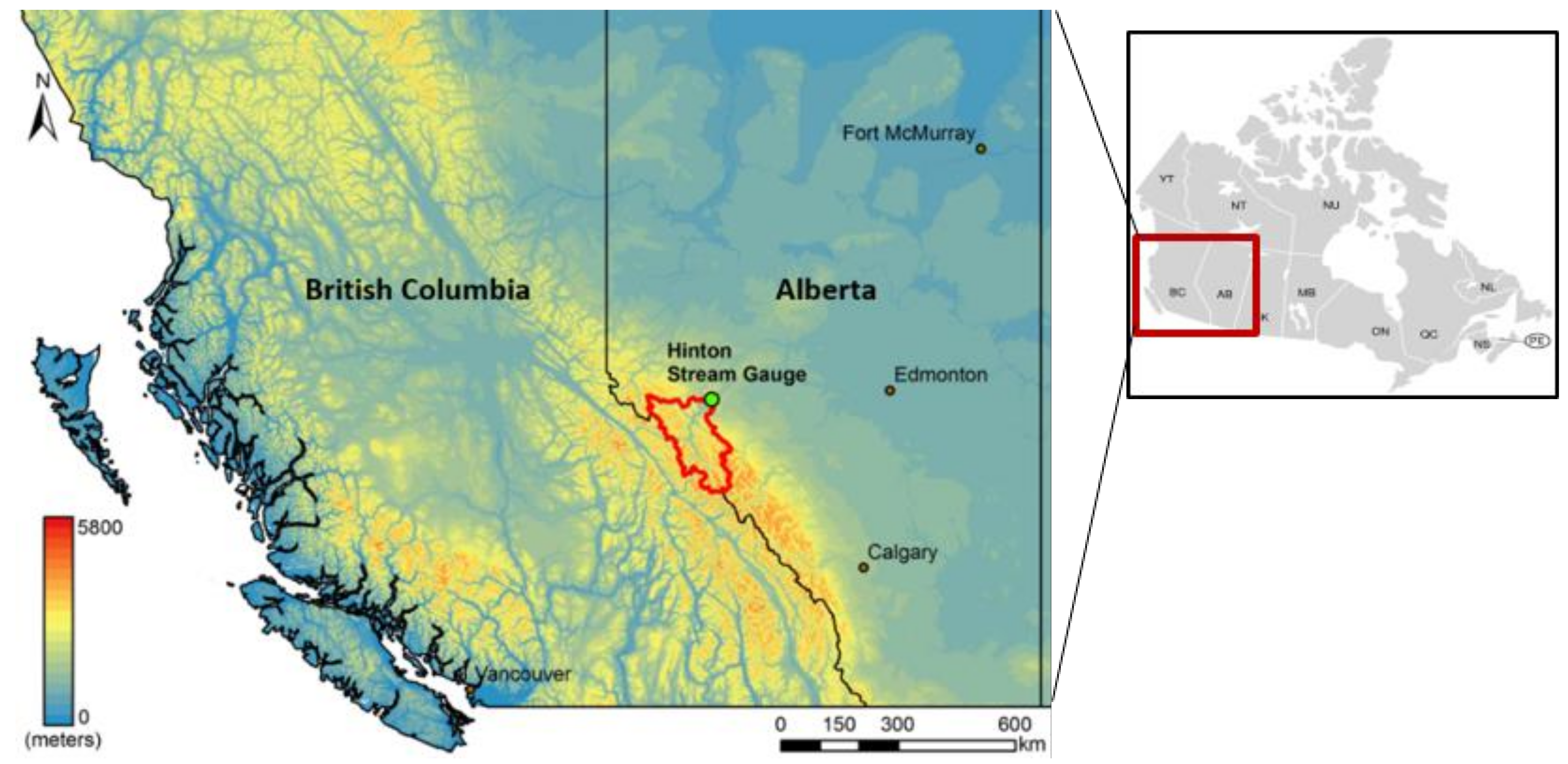
The focus of this study is the Upper Athabasca River Basin (UARB) above Hinton, located between 52°07′ N and 53°29′ N latitude (Figure 1). The 9760 km2 study basin is almost entirely located within the mountainous topography of the Rocky Mountains, with elevations ranging from 960 m to 3740 m asl (based on the Canadian Digital Elevation Model with 0.75 second (~20 m) resolution elevation data, geogratis.gc.ca). The basin experiences a subarctic climate with coniferous forests up to a 2200 m elevation. The mean annual precipitation in the basin is around 638 mm, with 47% falling as snow, and the mean monthly temperature ranges from around −10 °C in January to over 11 °C in July, with the mean annual value averaging around −0.29 °C over the 2000–2010 period (based on Natural Resources Canada gridded meteorological data, described in Section 2.2). Runoff in the region is snowmelt dominated, with low winter flows followed by the onset of snowmelt in late April or May. The flow typically peaks in June or July before gradually declining back to winter low flow. Glaciers are present at upper elevations, with glacial ice covering around 3% of the basin area.
2.2. Historical Climate, Snow, and Streamflow Data
The Natural Resources Canada gridded temperature and precipitation data product (NRCANmet) was used to drive the model over the calibration (2000–2005) and validation (2006–2010) periods. This product utilizes a tri-variate thin plate smoothing spline to interpolate temperature and precipitation from Environment Canada weather stations throughout Canada down to a 300 arc second grid (~10 km) [22]. Daily discharge data to calibrate and validate the hydrological model at the hydrometric station near Hinton, a town on the Athabasca River just downstream from Jasper National Park, were obtained from Environment Canada’s hydrometric database HYDAT (https://www.canada.ca/en/environment-climate-change/services/water-overview/quantity/monitoring/survey/data-products-services/national-archive-hydat.html accessed on 4 October 2017).
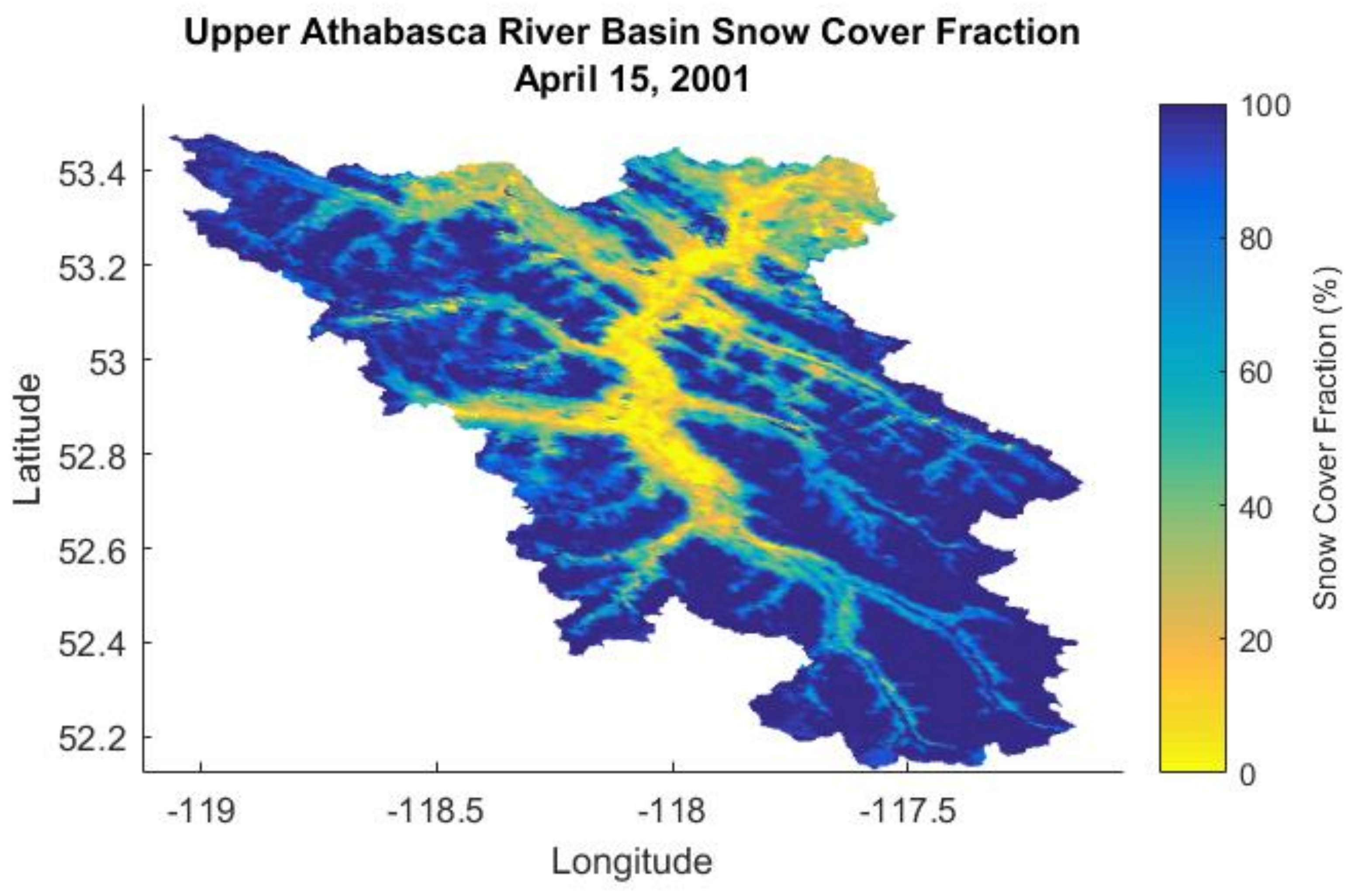
Information on snow cover area used as the model input was extracted from the MODIS imagery [23]. Multiple MODIS snow cover products are developed by the National Snow and Ice Data Center (NSIDC), including the MOD10A1 product, which provides daily subpixel snow cover fractions (the fraction of an area that is covered in snow) at a 500 m resolution. However, frequent cloud cover hinders the use of satellite imagery for measuring snow cover in the winter months. Hence, this study used the processed snow cover data that temporally interpolated the MOD10A1 snow cover product to fill in cloud-covered pixels using a cubic smoothing spline [24]. Still, the infrequent imagery makes it difficult to distinguish between the stable seasonal snowpack and shorter-term transitory snow cover. The 500 m resolution snow cover data were re-projected into the NAD83 (CSRS) 10TM (Forest) cartographic system at a 250 m resolution using nearest neighbor sampling (Figure 2). Glacier area within the model was set to the minimum observed MODIS SCA during the study period (2000–2010), and glacier outlines for the study region obtained from the Global Land Ice Measurements from Space (GLIMS) inventory were used for comparison with this estimate [25,26].
2.3. The Snowmelt Runoff Model (SRM)
The SRM computes runoff using the following equation:
The runoff Q on day n (Qn) is calculated from the individual contributions of snowmelt, rainfall, and recession from the previous day’s discharge. The rainfall and snowmelt contributions are summed over each elevation band i. Snowmelt for each zone is calculated using the mean daily temperature over the zone, Ti, the degree day factor (DDF), ai, and multiplying by the snow-covered area (SCAi). Rainfall contribution for each zone is calculated using the rainfall depth Pi and multiplying by the rainfall contributing area (RCAi). The runoff coefficients for both snow and rain (CSi and CRi) in Equation (1) account for losses due to evaporation and sublimation, and their optimum values are identified through model parameter calibration. Before the snowpack becomes ripe, rain on snow is assumed to become part of the snowpack, and RCAi is the zonal area excluding SCAi. Once ripe, rain on snow contributes to runoff immediately, thus, RCAi no longer excludes SCAi. However, the retention of surface melt by the snowpack is not explicitly accounted for in the SRM. Instead, the date on which the snowpack becomes ripe is set as a calibration parameter. Precipitation is partitioned into rain or snow based on the critical temperature parameter (Tc, not appearing in the above equation), which is also set during calibration. If the zonal temperature is below the critical temperature, precipitation is determined to fall as snow, and does not contribute immediately to runoff. Accumulated snow due to precipitation is tracked until positive temperatures release the stored water content to contribute to runoff. SCAi is set to 100% when a zone has snow in storage, such that snowmelt occurs over the entire elevation zone where there is snow in storage. Snow storage is only intended to capture short-lived snowfall events during the melt season with the use of remotely sensed imagery intended to capture the accumulated winter snowpack. As such, snow storage is only tracked between April 1 and October 31. The SRM handles runoff routing through the recession coefficient k, which expresses the decline in discharge during periods with no snowmelt or rainfall, and transforms the daily influx of water into runoff. Therefore, the recession coefficient determines the responsiveness of the basin, i.e., how quickly the flow is generated in response to rainfall or snowmelt, and how quickly flow recedes in their absence. The higher the recession coefficient, the less responsive the hydrograph will be. The basin response will vary depending on basin conditions. To account for the nonlinear variation in the basin response, the recession coefficient k is given by Equation (2), where it is a function of the recession parameters x and y. Optimum recession parameters are determined through model calibration.
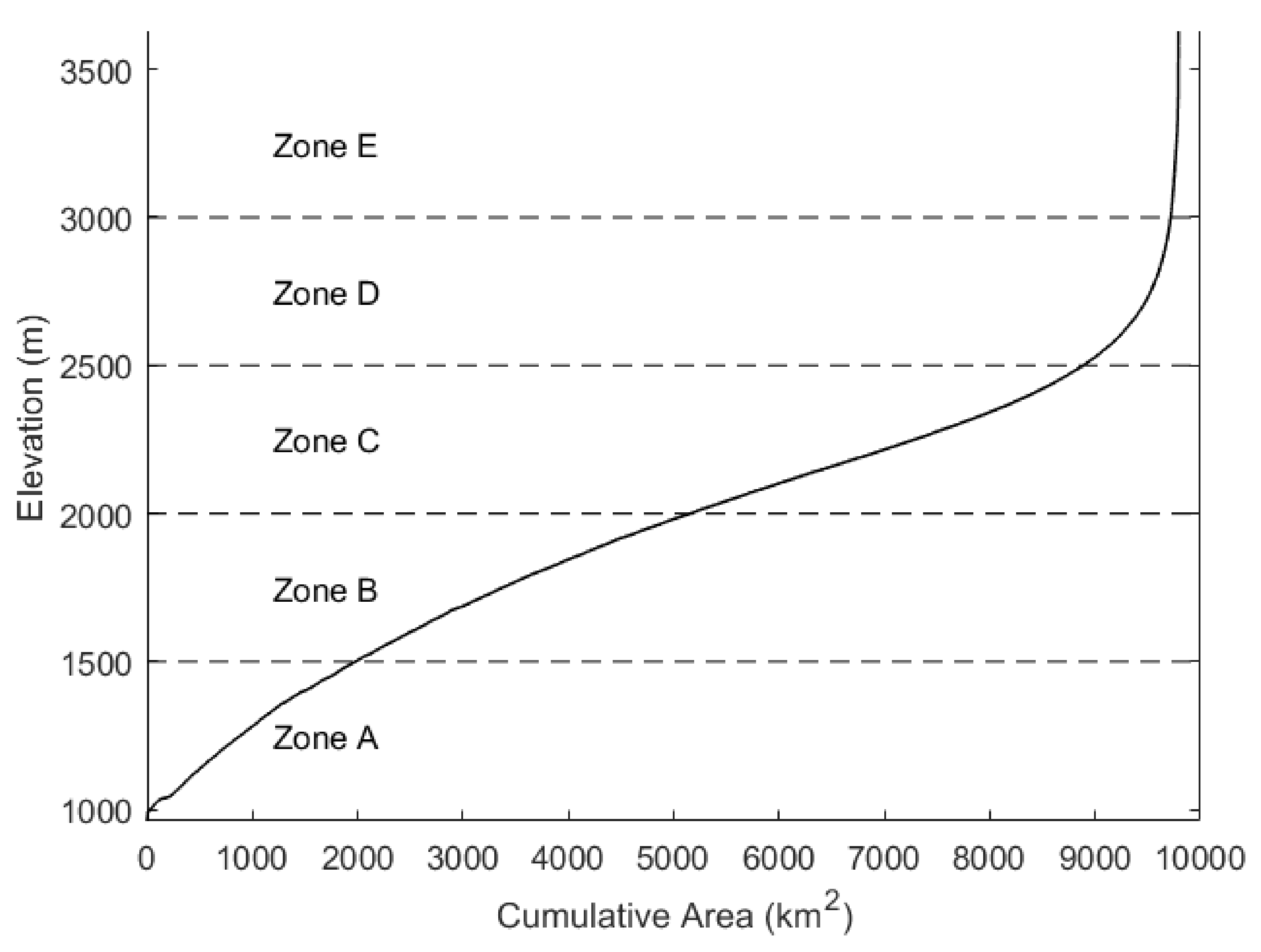
A more detailed description of the SRM can be found in Martinec et al. [15]. Building upon the work of Fitzharris and Sirguey [24], we implemented the SRM in MATLAB and applied the model for simulating runoff in the UARB at Hinton. The basin was divided into five elevation bands at 500 m intervals (Figure 3), with each variable averaged over the elevation zone to produce the zonal average temperature, precipitation, and snow cover values for each day. Calculated daily temperature lapse rates varied from −8.5°C/km to 7°C/km, with a mean of −4.5°C/km. The precipitation lapse rate varied from −12 mm/km to 232 mm/km, with a mean of 17 mm/km.
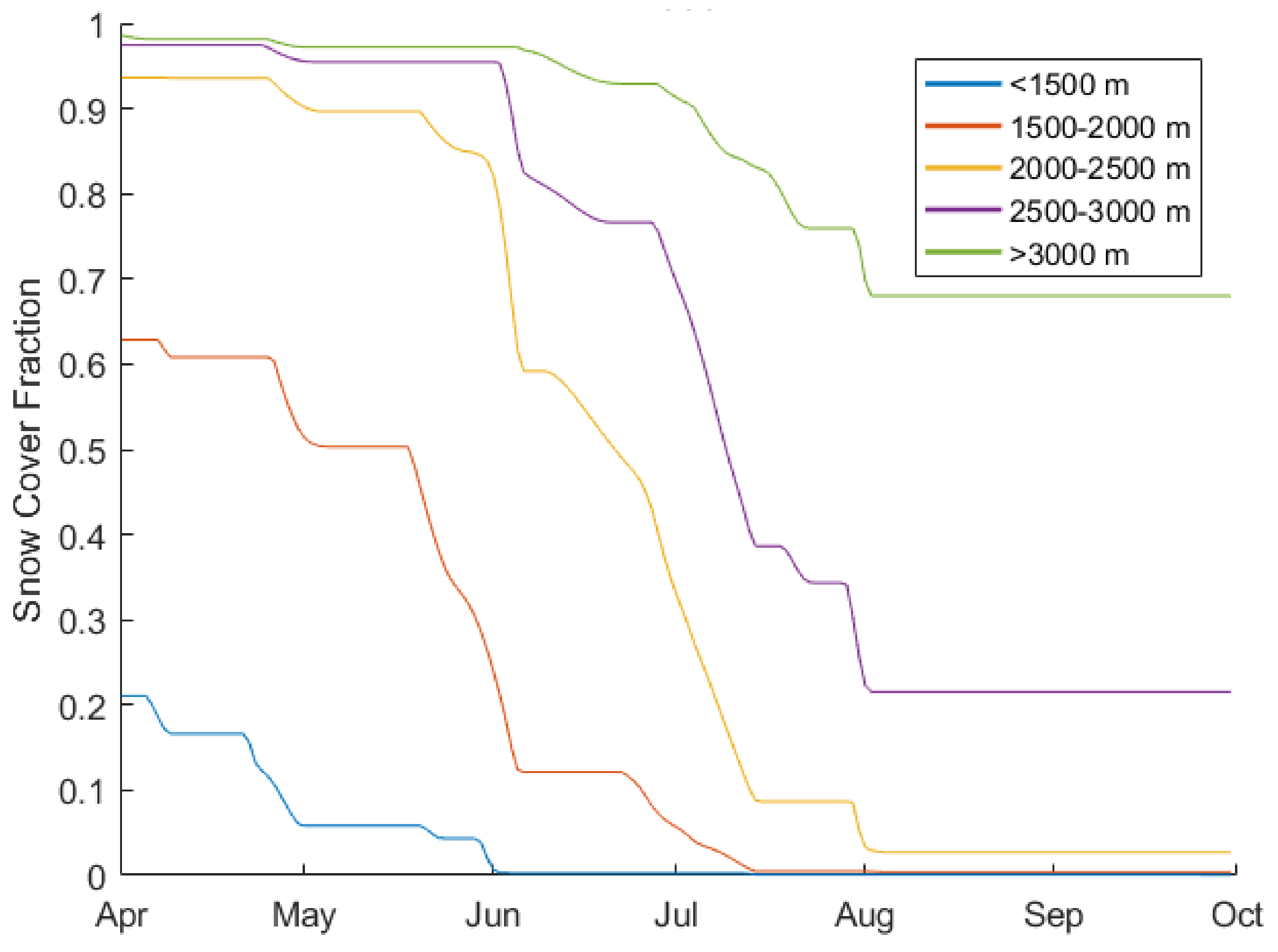
Before the SCA data from the satellite observation are used as the input into the SRM model, any spikes in the snow cover area during the melt season are removed. Specifically, following April 1 of each year, any increases in SCA are set to the value prior to the increase for each elevation band, such that snow cover never increased in extent and the snow cover fraction is monotonically decreasing (Figure 4). This is done because snowfall events during the melt season are simulated and accounted for by the SRM from meteorological data rather than satellite observations. Removing melt season snowfall events adjusts snow cover depletion curves to the pattern of melt corresponding to the base snowpack.
The DDF tends to be larger at higher elevations due to the increased relative contribution of radiation [14], and tends to be higher for glaciers due to the lower albedo of ice relative to snow, contributing more to its elevation dependency. DDF values may be determined through snow pillow or snow lysimeter measurements; an empirical relationship with snow density [27]; or based on energy balance modeling that has shown seasonal variation in the DDF to follow a sinusoidal pattern [28]. In the absence of physical measurements, the DDF may instead be chosen based on experience from other studies in the same geographical area or calibrated using the measured discharge (e.g., [29]). As no appropriate data were available for this region, the optimal DDF was determined through model calibration. Three approaches to handling spatial variability in the DDF were examined: a lumped DDF that does not vary spatially; a DDF with different values for glaciated and non-glaciated areas; and a zonal DDF with different values in each elevation band. The glacier-covered area was assumed to be equal to the minimum observed SCA over the study period. The glacier DDF was scaled from the snow DDF for simplicity, as it was expected to follow a similar seasonal variation. Besides, two approaches were examined to handle the temporal variability in the DDF: calibrating the DDF individually for each month, as is the standard approach in the SRM, and varying the DDF sinusoidally between maximum and minimum values on the summer and winter solstices, respectively (e.g., [28,30]).
2.4. SRM Model Calibration
The SRM parameters identified for calibration are listed in Table 1. Model calibration was implemented using the Markov Chain Monte Carlo (MCMC) procedure that utilizes a random walk technique to efficiently explore the parameter space [31]. The Metropolis−Hastings algorithm as described by Braswell et al. [32], which is an MCMC method, was implemented in this study using code made available by Zobitz et al. [33]. The algorithm incorporates the user’s knowledge of the system being modeled through the prior distribution of model parameters. The prior distribution represents the probability of parameter values based on existing knowledge of the system. Typically, the prior distribution of parameter values is assumed to be uniformly distributed between minimum and maximum allowable values [33]. The MCMC optimizes the model fit by randomly perturbing one parameter at a time within the range of allowable values until the best model fit is reached. The model fit was assessed using the Nash Sutcliffe Efficiency (NSE). The NSE can range from −∞ to 1, with 1 indicating a perfect fit between model results and observations. The NSE is computed by:
where and are the observed and modeled runoff values, respectively, and is the mean of the observed runoff values over the modeled period. Additionally, the model performance was evaluated by using the percent bias (PBIAS), though this measure was not utilized during calibration. The PBIAS is computed by:
During each iteration, the new parameter value is accepted if the model fit was improved. New parameter values with a worse model fit are also randomly accepted, with an inverse relationship between the decrease in model fit and the probability of acceptance to help prevent convergence on local rather than global optima. To attain the global optimum, the model parameters are also initialized at multiple chains of random starting points. The chains with the selected model fits are used as the starting point for a new chain in the iteration. The distance by which each parameter is perturbed is adjusted each iteration to obtain a specified acceptance rate of the new parameter values. As the chain progresses, the parameter perturbation distance is decreased as the random walk narrows in on an optimum value. In this way, the MCMC produces a set of accepted values, as well as their posterior distribution.
Three Markov chains were initialized for each calibration run, with a final chain of 10,000 iterations being run, starting from the best of the initial chains. Multiple calibrations were performed for each model set up to confirm that they converged near the same optimum. The NSE was used as the objective function for the calibration, and the parameter set with the best model fit (the maximum NSE) over the model calibration period was selected. The optimum model parameter sets for each case were used to test the model’s performance over the calibration and validation periods.
2.5. Future Climate Data
The potential impacts of climate change on the UARB runoff were examined using precipitation and temperature projections from six global climate models (GCMs) from the Climate Model Inter-Comparison Project Phase 5 (CMIP5) corresponding to the representative concentration pathways 8.5 (RCP8.5) scenario. RCP8.5 was chosen to examine the impacts of a worst case emissions scenario without substantial mitigation of greenhouse gasses, where emissions will continue to rise almost at the current rate throughout the twenty-first century. The six GCM models are CNRM-CM5.1, CanESM2, ACCESS1, INM-CM4, CSIRO-Mk3.6.0, and CCSM4 [34]. Since the GCMs have a low spatial resolution (~1° to 2.8°), they were statistically downscaled (SD) to a 10 km special resolution by the Pacific Climate Impacts Consortium (PCIC) [35]. The Bias Correction Spatial Downscaling (BCSD; [36]) and Bias Correction/Climate Imprint (BCCI; [37]) methods were used with the NRCANmet dataset for the 1951–2010 period as the downscaling target, resulting in 2X6 GCMs. Seasonal temperature and precipitation changes between the 2041–2070 and 1971–2000 periods corresponding to each of the GCMs and downscaling techniques as calculated by Dibike et al. [34] were applied to the 2000–2010 baseline data to compute future temperature and precipitation data and to drive hydrological model projections. Since 2000–2010 was used as the baseline period in this study, the 70-year difference between 2041–2070 and 1971–2000 roughly translated to the future climate scenario representing the 2070–2080 period.
2.6. Climate Change Impacts on Future Runoff
While the use of remotely sensed snow cover information improves accuracy in SRM modeling for the historical period, this approach has shortcoming for future projections, where expected changes in snow cover area resulting from reduced accumulation in winter and more rapid melt under warmer temperatures has to be estimated. The methodology for predicting the melt period snow cover area under future climates is based on establishing a relationship between the snow cover fraction and cumulative melt depth during the melt period using historical data. The cumulative melt depth is calculated for each day starting from April 1, using positive degree days and the calibrated DDF from historical data. The cumulative melt depth is plotted against the observed SCA, establishing the historical relationship between these variables. To project the future SCA, the cumulative melt depth is calculated from the future climate data, and the SCA is determined based on the historical melt depth/SCA relationship. Thus, if twice as much melt is calculated to have occurred by May 1 for the future climate relative to the baseline period, the SCA on May 1 is set to the SCA on whichever date historically had twice the melt depth of May 1 (e.g., May 15).
Moreover, potential change in winter accumulation of snow in the future period was accounted for by first calculating the SWE on April 1 by simulating snowpack over the winter months (October–March). As with during the melt season, if the zonal temperature was below the critical temperature, precipitation was determined to fall as snow, and was added to snow storage for that zone. Similarly, melt was calculated from positive degree days and subtracted from this snow storage, and, at the end of the winter period, the April 1 SWE was obtained. This April 1 SWE was calculated using both the historical and future temperature and precipitation data. The difference between the historical and future April 1 SWE was then added to the cumulative melt depth of the future period and used in projecting the new SCA. A more detailed description of this procedure is available from Martinec et al. [15]. Similarly, potential changes in the glacier area were accounted for when simulating climate change impacts. However, since glacier dynamics are not explicitly modeled in this study, the 200 m resolution glacier area product by Clarke et al. [38] was applied in adjusting the glacier area for the Upper Athabasca watershed using the percentage reduction in the glacier area at each elevation band between the historical (2000–2010) and future (2070–2080) time periods and applying it to the SRM. Finally, after the SRM was run for the future period using the adjusted climate variables and SCA depletion curves, simulated flows were compared to the corresponding model results for the baseline climate.
3. Results and Discussion
3.1. Model Calibration and Validation
The SRM model for the UARB was calibrated with the MCMC method using observed discharge data at the Hinton station for the years 2000 to 2005 and validated over the 2006 to 2010 period. The calibration and validation periods displayed sufficient variability in meteorological and snow conditions to represent the inter-annual variability of discharge from the basin. The NSE corresponding to the range of possible model parameters was examined for each DDF approach over both the calibration and validation periods (Figure 5). The best calibration and validation results over the historical baseline period are presented in Table 2.
As expected, the NSE values for the validation period were mostly lower than those of the calibration period. The results also showed that the two temporal DDF approaches (monthly and sinusoidal variation) gave a comparably better model fit over both the calibration and validation periods. The lumped approach, where the DDF value did not vary over the basin, captured the seasonal flow pattern well, but missed flow peaks and troughs in favor of a smoothed hydrograph with the best NSE values for the calibration and validation datasets ranging between 0.82 and 0.89. The inclusion of spatial variation in the DDF, either through an independent DDF for each elevation band or a separate glacier DDF, resulted in a notable improvement in the model fit over the lumped approach with the best NSE values over the calibration and validation datasets ranging between 0.83 and 0.92 (Table 2). The mean absolute flow volume error was highest for the zonal DDF approach (6.0% with the monthly DDF, 6.1% with the sinusoidal DDF) and lowest with the glacier DDF approach (4.2% with the monthly DDF, 4.5% with the sinusoidal DDF) and the lumped sinusoidal DDF approach (3.9%).
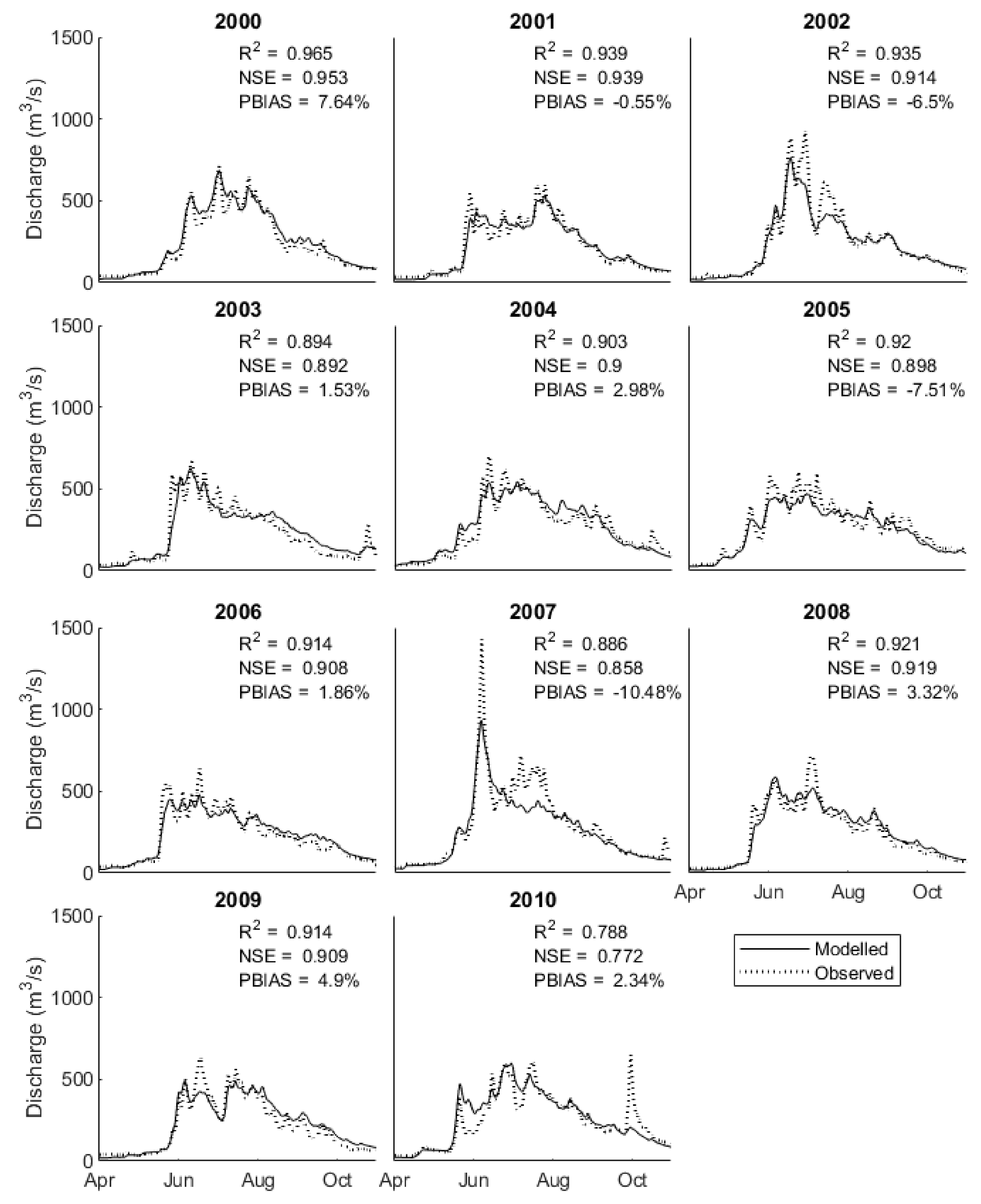
While the overall model performance was very good, the model sometimes failed to capture certain aspects of the observed hydrograph, regardless of the DDF approach (Figure 6). The sub-freezing temperatures experienced in the UARB over the winter months result in little meltwater production or rainfall to maintain flows throughout the winter; model results underestimated flows during the winter months. This is because of the simplified representation of the recession coefficient as a function of discharge, with the basin more responsive at higher flows when overland flow dominates, and less responsive at lower flows when ground water contributes a larger proportion of flow. Some flow peaks are missed or underestimated during the months of June and July. The most significant missed flow peaks occur coincidentally with the SCA reaching its minimum in June (2009) or July (2002, 2007, 2008). Flow underestimation associated with below-average snow cover also occurred in June 2005 and 2006. This may be a result of the MODIS snow cover product that has been found to underestimate snow cover, particularly when the snow cover fraction is below 20% [39,40]. A persistent bias could be corrected through calibration of the DDF or runoff coefficient, but greater underestimation at a lower snow cover fraction would lead to flow underestimation when the SCA is small. This SCA underestimation may also be responsible for the missed June and July flow peaks. Flow overestimation occurred in 2000 and 2010, both years with above-average snow cover in June and July.
3.2. Parameter Sensitivity and Model Uncertainty
The posterior distributions of model parameters were examined to evaluate the model uncertainty (Figure 7). The recession coefficients (x and y) had the narrowest posterior distributions, as they were the most sensitive parameters, where a small perturbation had substantial impact on the hydrograph. While higher y values increase hydrograph responsiveness at higher flows relative to lower flows, higher x values increase responsiveness across all flows. The runoff coefficients (cs and cr) were both moderately constrained, with the rainfall runoff coefficient generally constrained to the lower end of its range, while the snowmelt runoff coefficient was constrained to the middle of its range. For the monthly DDF with the glacier approach, a seasonal progression could be seen in the posterior distributions of DDF values, with the likelihood value increasing from 0.3 cm/°C/day in May to just under 0.6 cm/°C/day in July. The parameters were poorly constrained outside of this period, as the lower contribution of snowmelt to discharge renders the model less sensitive to the perturbation of these parameters. The sinusoidal DDF approach is advantageous in this regard, constraining the DDF to a realistic seasonal progression. The June 21 maximum DDF value of the sinusoidal approach places its seasonal progression slightly ahead of the monthly approach, where the maximum occurs in July. The glacier DDF peaked in likelihood near the upper limit of its permitted range. The glacier DDF was limited to 2 cm/°C/day, the maximum of the observed and calculated DDF values of the studies summarized by Hock [14]. Critical melt temperature (Tc) displayed a broad posterior distribution, with a preference towards higher values. Higher critical temperatures decreased flow earlier in the year (April/May) in favor of the warmer months (July/August). When the critical temperature was high, the snow ripeness date parameter (SRD) had little effect on the hydrograph. At lower critical temperatures, a late ripeness date served a similar function to a higher critical temperature by reducing discharge from early season rainfall events.
3.3. Projected Changes in Precipitation and Temperature
Projected changes in seasonal temperature and precipitation over the region between the 2000–2010 baseline and the 2070–2080 future period are presented in Table 3. While the result showed inter-model variability in the projected changes, most models projected increases in both temperature and precipitation over the region, with the highest temperature change being in the winter and the highest precipitation change being in the spring, though some models projected decreasing precipitation in summer. The ensemble mean seasonal changes for temperature varied between 2.4 °C in spring and 4.5 °C in winter, while that of precipitation varied between 1.8% in the summer and 22.8% in the spring.
3.4. Projected Snow Cover Area and Glacier Extents
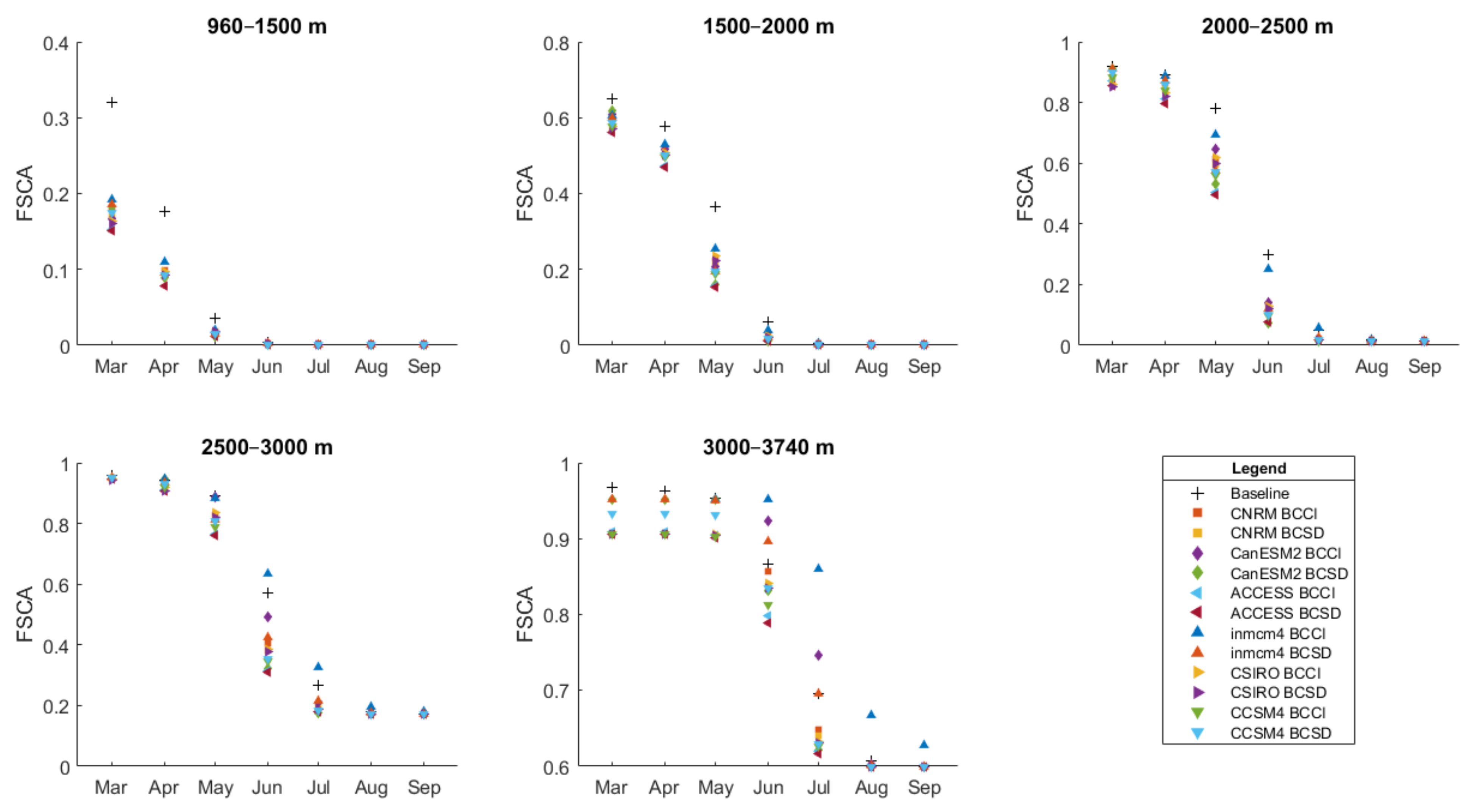
The projected temperature and precipitation corresponding to the different GCM/SD models generally resulted in a decreased SCA for the lower elevation bands (below 2500 m), but the responses were more variable at higher elevations (Figure 8). This increased variability at higher elevations results from temperatures remaining sufficiently cool despite future warming such that increased snowfall from higher precipitation outweighs increased melt in some projections. Compared to the baseline period, the projected SCA at the start of the melt season (April 1) was reduced by 40% to 53% in the 960–1500 m elevation band, whereas declines were no more than 6% in the 3000–3740 m elevation band. All GCM/SD projections resulted in a reduced SCA at 2500–3000 m, except one (inmcm4/BCCI) that showed increased snow cover from June onward. The projections driven by CanESM2/BCCI, inmcm4/BCSD, and inmcm4/BCCI depicted increases in snow cover at the 3000–3740 m elevation band, while the rest showed decreased snow cover. The CanESM2 and inmcm4 driven projections provided the largest increases in precipitation, leading to increased snowfall that accounted for the increase in the SCA at a high elevation. Additionally, the inmcm4-driven simulation projected the least warming, which, combined with the increase in precipitation, explained its position with the highest SCA.
The month experiencing the greatest percentage decline in the SCA was shifted progressively later in the year with increasing elevation: May experienced the greatest decline in the SCA below 1500m (45–68% decrease at 960 to 1500 m), June at 1500–2000 m, and June or July above 2000 m. Little or no decline occurred after August, as the methodology for calculating snow cover under the future climate does not allow the SCA to drop below the minimum observed SCA for that zone. While the largest percentage change in the SCA occurred between May and July (depending on the elevation zone and GCM/SD), the largest absolute change in the SCA generally occurred in April or May due to more extensive snow cover in these months. To account for the reduction of the glacier area under a warming climate, the percentage changes in the modeled glacier area from Clarke et al. [38] between 1971–2000 and 2041–2070 were calculated for each elevation band and averaged over the six GCMs used in that study (Table 4).
3.5. Projected Changes in Runoff
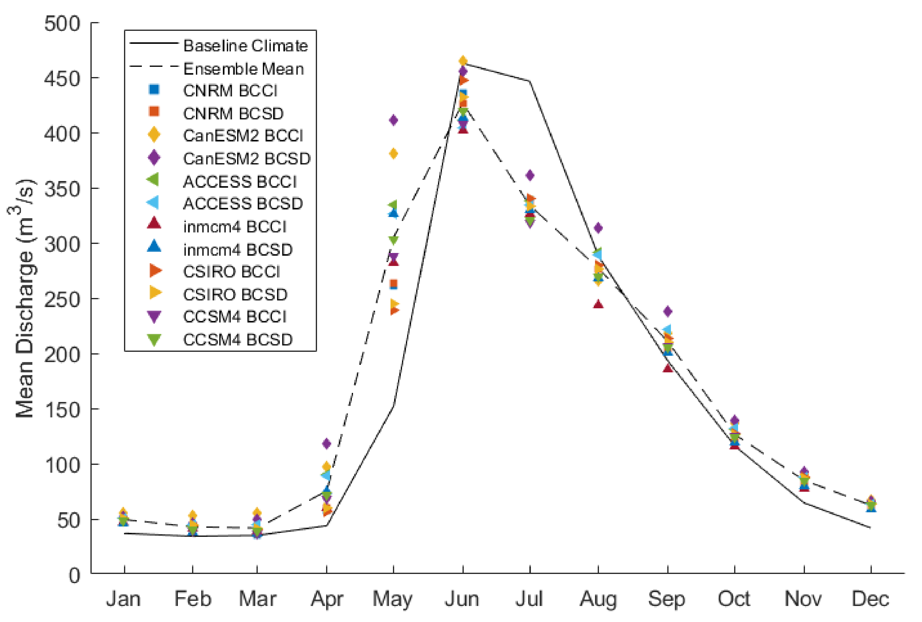
Given its consistent performance during the calibration, validation, and realistically constrained parameter values, the SRM with the sinusoidal seasonal variation and glacier DDF approach was used for simulating future runoff. The calibrated SRM was run using the modified precipitation, temperature, and SCA data corresponding to each of the twelve GCM/SD combinations. The results showed that the mean annual discharge (MAD) increased for all climate change projections, with the exception of inmcm4/BCCI (Figure 9, Table 5). Changes in MAD ranged from −3 m3/s (−2%) for inmcm4/BCCI to +36 m3/s (+22%) for the CanESM2/BCSD, deviating from the baseline climate MAD of 160 m3/s. The ensemble mean change in MAD was +10 m3/s (+6%).
Model results also showed a shift to an earlier spring freshet consistent with observed trends [4] and the expected consequence of a warmer climate [2]. Increases in flow occurred in the months of October through May, resulting from warmer temperatures and the consequent increase in cold season rainfall and snowmelt. May was projected to experience the largest increase in discharge of any month, regardless of GCMs/SD, ranging from an increase of 54% (CSIRO BCCI) to 164% (CanESM2 BCSD), with the ensemble mean monthly increase being 97%, almost doubling the baseline flow for the month. Subsequently, the earlier depletion of the seasonal snowpack mostly produced lower flows in June through August, with July experiencing the greatest absolute decline in ensemble mean flows (−77.4 m3/s or −19%) of any month. In general, this results in a reduction in the season variation of flow in the UARB, with decreased flows during the high flow summer months (June, July, and August) and increased flows for the rest of the year. While an overall shift toward an earlier freshet was projected, June still remained the month with the highest flow for the 2070–2080 period, although its magnitude was slightly reduced from its baseline value.
Historical runoff trends for the Athabasca River near Jasper showed statistically significant decreases in flow for the months of July, August, and September over the period of 1914–2005 [4]. Our results showed similar future declines in July and August flows, but little change or even slight increases in September. The projected decline in June flow, a month where no significant decline has been observed historically, showed progressively earlier depletion of the future snowpack. Snow cover over the baseline period (2000–2010) reached its minimum in August, and the methodology for simulating the future SCA precludes the modeled SCA below the observed minimum. This limitation would result in an overestimation of flows in late summer when the SCA could be expected to decline even below its historically observed minimum.
The runoff projection accuracy may be limited by the simplified formulation of the SRM. While the model performed well during the calibration and validation periods, the model performance may decline as the climate conditions drift farther from those experienced during the calibration period. For example, the DDF could drift over time due to changing relative contributions to the snowpack energy balance. However, a study comparing degree–day and mixed degree–day energy balance snowmelt models in climate change projections for three catchments in Quebec found comparable performance between the two methods [41]. The accuracy of SCA projections and the use of a set change in the glacier area across all climate change scenarios could be other sources of uncertainty. Besides snowmelt, processes such as the freezing and thawing of soil and evapotranspiration may impact effective model parameters under a changing climate. Soil ice content controls infiltration rates and impacts soil thermal conductivity and heat capacity [42], and changing soil ice content will influence the delivery of snowmelt to watercourses. Evapotranspiration is accounted for through the runoff coefficient parameter in the SRM; this parameter is held constant during runoff projections, though this is likely not realistic, as warming temperatures will increase evapotranspiration rates.
The modeled increase in the MAD is not consistent with the observed historical decreasing trend by Bawden et al. [43]. However, the historical decreasing trend may not continue in the future because of a projected increase in precipitation, and, in this regard, our results are consistent with other modeling studies, such as Eum et al. [44] and Toth et al. [45], which utilized more physical process-based hydrological models (VIC and WATFLOOD, respectively) and projected the increased MAD, increased spring flows, and decreased summer flows. Our projected increase in the MAD of 6% is only slightly less than the 8.4% increase projected by Eum et al. [44]. Projected changes in annual and seasonal flows at Hinton in Eum et al. [44] lie within the range of projected flows over the 12 GCMs/SD used in our study. For example, while Eum et al. [44] projected an ensemble mean increase of 88% in spring flows, we projected a corresponding increase of 97%.
4. Conclusions
A Snowmelt Runoff Model (SRM) was applied to simulate runoff for the Upper Athabasca River Basin at Hinton over the 2000–2010 baseline period, using the MOD10A1 snow cover product and testing multiple approaches for handling spatial and temporal variation in the degree day factor (DDF). After successful calibration and validation over the baseline period, the model was used to project future change in the basin’s runoff. Model calibration/validation results demonstrated that accounting for spatial variation in the DDF improved model performance and better simulated individual runoff peaks over using a lumped DDF. The use of a separate DDF for glaciated and non-glaciated areas performed on par with the typical zonal approach with separate DDFs for each elevation band. These results indicate the higher DDF for glacial ice can account for much of the elevational dependence of the DDF. Scaling the glacial DDF from the snow DDF was found to provide comparable results to calibrating each separately, as both follow a similar seasonal pattern. The seasonal progression in the melt factor was found to be better captured by sinusoidally varying the DDF between a summer maximum and winter minimum. Constraining the DDF to a sinusoidal pattern generated more reliable results over the validation period than freely varying the DDF on a monthly basis. Parameter sensitivity analysis showed that DDF values in the monthly model were poorly constrained in months where snowmelt contributions were relatively low. In addition to the DDF, the runoff and recession coefficients are found to be very sensitive parameters. While the SRM benefits from its simplicity and few required input variables, this study demonstrated that incorporating some process understanding about hydrological processes (e.g., glacial melt) could be advantageous to the robustness of model results under varying hydrological conditions.
The future hydrologic responses of the basin were examined using climatic drivers from six GCMs downscaled with two SD methods under the RCP8.5 scenario. The snow cover area is projected to decline, with the largest declines occurring at lower elevations. In general, the river flow is projected to decrease during the summer higher flow months, while it is projected to increase for the rest of the year. Results show a substantial increase in projected runoff for the month of May, followed by that of April. Increased runoffs from October through March are smaller relative to the increases in April and May, but larger relative to the historically low flows over these months. In addition to the largest increases in flow, April and May experience the largest declines in snow cover area. The shift towards an earlier freshet and corresponding earlier depletion of the spring snowpack result in lower summer flows, with June, July, and August experiencing decreases. Despite the substantially increasing May and declining June runoff, June is still projected to remain the highest flow month. These projections are consistent with observed historical trends and other modeling studies.
In general, the SRM is found to be a relatively simple tool for hydrological modeling of alpine watersheds using remotely observed snow cover information, and it can be extended for assessing the potential impact of a changing climate. The validity of calibrated parameter values may decline outside of the climatic conditions for which the model was calibrated; future research could examine the robustness of SRM parameters for changing climate. A study examining the transferability of parameter values between watersheds could enable the application of the SRM in modeling runoff in ungauged basins. Another potential application of the SRM is in operational short-term flood forecasting, which has been the focus of several previous studies. Future work could investigate setting the DDF as a function of albedo, which could account for both temporal and spatial variation in the DDF. Differences in the DDF between forested and alpine areas could also be investigated.
Author Contributions
Conceptualization, K.S., Y.D., and T.P.; Methodology, K.S., Y.D., R.R.S., and T.P.; Data analysis, K.S.; supervision, Y.D. and T.P.; Original draft preparation, K.S. and Y.D.; Review and editing, K.S., Y.D., R.R.S., and T.P.; funding acquisition, T.P. All of the co-authors reviewed the manuscript prior to and during the submission process to the Water-MDPI Journal. All authors have read and agreed to the published version of the manuscript.
Funding
This work was partially supported by a Discovery Grant from the Natural Sciences and Engineering Council of Canada (NSERC) to one of the co-authors and Environment and Climate Change Canada’s Climate Change and Adaptation program.
Data Availability Statement
Not applicable.
Acknowledgments
We thank Blair Fitzharris and Pascal Sirguey for supplying the temporally interpolated MODIS snow cover product.
Conflicts of Interest
The authors declare no conflict of interest. The funders had no role in the design of the study; in the collection, analyses, or interpretation of data; in the writing of the manuscript, or in the decision to publish the results.
References
- Ferguson, R.I. Snowmelt runoff models. Prog. Phys. Geogr. 1999, 23, 205–227. [Google Scholar] [CrossRef]
- Barnett, T.P.; Adam, J.C.; Lettenmaier, D.P. Potential impacts of a warming climate on water availability in snow-dominated regions. Nature 2005, 438, 303–309. [Google Scholar] [CrossRef]
- Arnell, N.W. Climate change and global water resources. Glob. Environ. Chang. 1999, 9, S31–S49. [Google Scholar] [CrossRef]
- Rood, S.B.; Pan, J.; Gill, K.M.; Franks, C.G.; Samuelson, G.M.; Shepherd, A. Declining summer flows of Rocky Mountain rivers: Changing seasonal hydrology and probable impacts on floodplain forests. J. Hydrol. 2008, 349, 397–410. [Google Scholar] [CrossRef]
- Bonsal, B.; Shrestha, R.R.; Dibike, Y.; Peters, D.L.; Spence, C.; Mudryk, L.; Yang, D. Western Canadian freshwater availability: Current and future vulnerabilities. Environ. Rev. 2020, 28, 528–545. [Google Scholar] [CrossRef]
- Collins, M.; Knutti, R.J.; Arblaster, J.; Dufresne, J.L.; Fichefet, T.; Friedlingstein, P.; Gao, X.; Gutowski, W.J.; Johns, T.; Krinner, G.; et al. 2013: Long-term climate change: Projections, commitments and irreversibility. In Climate Change 2013: The Physical Science Basis; Contribution of Working Group I to the 5th Assessment Report of the Intergovernmental Panel on Climate Change; Stocker, F.T., Qin, D., Plattner, G.-K., Tignor, M., Allen, S.K., Boschung, J., Nauels, A., Xia, Y., Bex, V., Midgley, P.M., Eds.; Cambridge University Press: Cambridge, UK, 2003; pp. 1029–1136. [Google Scholar]
- O’Neil, H.C.L.; Prowse, T.D.; Bonsal, B.R.; Dibike, Y.B. Spatial and temporal characteristics in streamflow-related hydroclimatic variables over western Canada. Part 2: Future projections. Hydrol. Res. 2016, 48, 932–944. [Google Scholar] [CrossRef]
- Faurès, J.M.; Goodrich, D.C.; Woolhiser, D.A.; Sorooshian, S. Impact of small-scale spatial rainfall variability on runoff modeling. J. Hydrol. 1995, 173, 309–326. [Google Scholar] [CrossRef]
- Stahl, K.; Moore, R.; Floyer, J.; Asplin, M.; McKendry, I. Comparison of approaches for spatial interpolation of daily air temperature in a large region with complex topography and highly variable station density. Agric. For. Meteorol. 2006, 139, 224–236. [Google Scholar] [CrossRef]
- Feiccabrino, J.; Graff, W.; Lundberg, A.; Sandström, N.; Gustafsson, D. Meteorological knowledge useful for the improvement of snow rain separation in surface based models. Hydrology 2015, 2, 266–288. [Google Scholar] [CrossRef] [Green Version]
- Mott, R.; Vionnet, V.; Grünewald, T. The seasonal snow cover dynamics: Review on wind-driven coupling processes. Front. Earth Sci. 2018, 6, 197. [Google Scholar] [CrossRef]
- Lehning, M.; Fierz, C. Assessment of snow transport in avalanche terrain. Cold Reg. Sci. Technol. 2008, 51, 240–252. [Google Scholar] [CrossRef]
- Hock, R. Glacier melt: A review of processes and their modelling. Prog. Phys. Geogr. Earth Environ. 2005, 29, 362–391. [Google Scholar] [CrossRef]
- Hock, R. Temperature index melt modelling in mountain areas. J. Hydrol. 2003, 282, 104–115. [Google Scholar] [CrossRef]
- Martinec, J.; Rango, A.; Roberts, R. Snowmelt Runoff Model (SRM) User’s Manual; New Mexico State University: Las Cruces, NM, USA, 2008. [Google Scholar]
- Rango, A.; Martinec, J. Revisiting the degree-day method for snowmelt computations. JAWRA J. Am. Water Resour. Assoc. 1995, 31, 657–669. [Google Scholar] [CrossRef]
- Debele, B.; Srinivasan, R.; Gosain, A.K. Comparison of process-based and temperature-index snowmelt modeling in SWAT. Water Resour. Manag. 2009, 24, 1065–1088. [Google Scholar] [CrossRef]
- Day, C.A. Modelling impacts of climate change on snowmelt runoff generation and streamflow across western US mountain basins: A review of techniques and applications for water resource management. Prog. Phys. Geogr. Earth Environ. 2009, 33, 614–633. [Google Scholar] [CrossRef]
- Mountain Research Initiative EDW Working Group; Pepin, N.; Bradley, R.S.; Diaz, H.F.; Baraer, M.; Caceres, E.B.; Forsythe, N.; Fowler, H.J.; Greenwood, G.; Hashmi, M.Z.; et al. Elevation-dependent warming in mountain regions of the world. Nat. Clim. Chang. 2015, 5, 424–430. [Google Scholar] [CrossRef] [Green Version]
- Tahir, A.A.; Chevallier, P.; Arnaud, Y.; Neppel, L.; Ahmad, B. Modeling snowmelt-runoff under climate scenarios in the Hunza River basin, Karakoram Range, Northern Pakistan. J. Hydrol. 2011, 409, 104–117. [Google Scholar] [CrossRef]
- Ma, Y.; Huang, Y.; Chen, X.; Li, Y.; Bao, A. Modelling snowmelt runoff under climate change scenarios in an ungauged mountainous watershed, Northwest China. Math. Probl. Eng. 2013, 2013, 1–9. [Google Scholar] [CrossRef] [Green Version]
- Hutchinson, M.F.; McKenney, D.W.; Lawrence, K.; Pedlar, J.H.; Hopkinson, R.F.; Milewska, E.; Papadopol, P. Development and testing of Canada-wide interpolated spatial models of daily minimum-maximum temperature and precipitation for 1961–2003. J. Appl. Meteorol. Clim. 2009, 48, 725–741. [Google Scholar] [CrossRef]
- Hall, D.K.; A Riggs, G.; Salomonson, V.V.; DiGirolamo, N.E.; Bayr, K.J. MODIS snow-cover products. Remote. Sens. Environ. 2002, 83, 181–194. [Google Scholar] [CrossRef] [Green Version]
- Fitzharris, B.; Sirguey, P. Building a Platform for Snowmelt Runoff Modelling in the Athabasca River Basin; Climate Management Ltd.: Lusaka, Zambia, 2014; Unpublished Report. [Google Scholar]
- Raup, B.; Racoviteanu, A.; Khalsa, S.J.S.; Helm, C.; Armstrong, R.; Arnaud, Y. The GLIMS geospatial glacier database: A new tool for studying glacier change. Glob. Planet. Chang. 2007, 56, 101–110. [Google Scholar] [CrossRef]
- Bolch, T.; Menounos, B.; Wheate, R. Landsat-based inventory of glaciers in western Canada, 1985–2005. Remote Sens. Environ. 2010, 114, 127–137. [Google Scholar] [CrossRef]
- Martinec, J. The Degree-Day Factor for Snowmelt Runoff Forecasting; IAHS Commission of Surface Waters, IUGG General Assembly of Helsinki: Potsdam, Germany, 1960; Volume 51, pp. 468–477. [Google Scholar]
- Anderson, E.A. Snow Accumulation and Ablation Model—SNOW-17; US National Weather Service: Silver Spring, MD, USA, 2006. [Google Scholar]
- Panday, P.K.; Williams, C.A.; Frey, K.E.; Brown, M.E. Application and evaluation of a snowmelt runoff model in the Tamor River Basin, Eastern Himalaya using a Markov Chain Monte Carlo (MCMC) data assimilation approach. Hydrol. Process. 2013, 28, 5337–5353. [Google Scholar] [CrossRef] [Green Version]
- Braun, L.N.; Grabs, W.; Rana, B. Application of a conceptual precipitation-runoff model in the Langtang Khola Basin, Nepal Himalaya. IAHS Publ. 1993, 218, 221–238. [Google Scholar]
- Smith, T.J.; Marshall, L.A. Exploring uncertainty and model predictive performance concepts via a modular snowmelt-runoff modeling framework. Environ. Model. Softw. 2010, 25, 691–701. [Google Scholar] [CrossRef]
- Braswell, B.H.; Sacks, W.J.; Linder, E.; Schimel, D.S. Estimating diurnal to annual ecosystem parameters by synthesis of a carbon flux model with eddy covariance net ecosystem exchange observations. Glob. Chang. Biol. 2005, 11, 335–355. [Google Scholar] [CrossRef]
- Zobitz, J.M.; Desai, A.R.; Moore, D.J.P.; Chadwick, M.A. A primer for data assimilation with ecological models using Markov Chain Monte Carlo (MCMC). Oecologia 2011, 167, 599–611. [Google Scholar] [CrossRef]
- Dibike, Y.; Eum, H.-I.; Prowse, T. Modelling the Athabasca watershed snow response to a changing climate. J. Hydrol. Reg. Stud. 2018, 15, 134–148. [Google Scholar] [CrossRef]
- Werner, A.T.; Cannon, A.J. Hydrologic extremes—An intercomparison of multiple gridded statistical downscaling meth-ods. Hydrol. Earth Syst. Sci. 2016, 20, 1483. [Google Scholar] [CrossRef] [Green Version]
- Maurer, E.P.; Hidalgo, H.G. Utility of daily vs. monthly large-scale climate data: An intercomparison of two statistical downscaling methods. Hydrol. Earth Syst. Sci. 2008, 12, 551–563. [Google Scholar] [CrossRef] [Green Version]
- Hunter, R.D.; Meentemeyer, R.K. Climatologically aided mapping of daily precipitation and temperature. J. Appl. Meteorol. 2005, 44, 1501–1510. [Google Scholar] [CrossRef]
- Clarke, G.K.C.; Jarosch, A.H.; Anslow, F.S.; Radić, V.; Menounos, B. Projected deglaciation of western Canada in the twenty-first century. Nat. Geosci. 2015, 8, 372–377. [Google Scholar] [CrossRef]
- Kult, J.; Choi, W.; Choi, J. Sensitivity of the snowmelt runoff model to snow covered area and temperature inputs. Appl. Geogr. 2014, 55, 30–38. [Google Scholar] [CrossRef]
- Déry, S.J.; Salomonson, V.V.; Stieglitz, M.; Hall, D.K.; Appel, I. An approach to using snow areal depletion curves inferred from MODIS and its application to land surface modelling in Alaska. Hydrol. Process. 2005, 19, 2755–2774. [Google Scholar] [CrossRef]
- Troin, M.; Poulin, A.; Baraer, M.; Brissette, F. Comparing snow models under current and future climates: Uncertainties and implications for hydrological impact studies. J. Hydrol. 2016, 540, 588–602. [Google Scholar] [CrossRef]
- Cherkauer, K.A.; Lettenmaier, D.P. Hydrologic effects of frozen soils in the upper Mississippi River basin. J. Geophys. Res. Space Phys. 1999, 104, 19599–19610. [Google Scholar] [CrossRef]
- Bawden, A.J.; Linton, H.C.; Burn, D.H.; Prowse, T.D. A spatiotemporal analysis of hydrological trends and variability in the Athabasca River Region, Canada. J. Hydrol. 2014, 509, 333–342. [Google Scholar] [CrossRef]
- Eum, H.-I.; Dibike, Y.; Prowse, T. Climate-induced alteration of hydrologic indicators in the Athabasca River Basin, Alberta, Canada. J. Hydrol. 2017, 544, 327–342. [Google Scholar] [CrossRef]
- Toth, B.; Pietroniro, A.; Conly, F.M.; Kouwen, N. Modelling climate change impacts in the Peace and Athabasca catchment and delta: I—Hydrological model application. Hydrol. Process. 2006, 20, 4197–4214. [Google Scholar] [CrossRef]
Figure 1.
Location map showing the topography of the study area and the UARB boundary located in western Canada (outlined in red).
Figure 1.
Location map showing the topography of the study area and the UARB boundary located in western Canada (outlined in red).

Figure 2.
An example of a snow cover map for the study area from the MOD10A1 snow cover product at a 250 m resolution.
Figure 2.
An example of a snow cover map for the study area from the MOD10A1 snow cover product at a 250 m resolution.

Figure 3.
Hypsometric curve for the study area (UARB) with the five elevation bands identified for this study.
Figure 3.
Hypsometric curve for the study area (UARB) with the five elevation bands identified for this study.

Figure 4.
Snow cover depletion curves corresponding to each elevation band in the UARB for the year 2000 (with melt Scheme 1 for each elevation band to account for the seasonal and elevational variation in the DDF [15]).
Figure 4.
Snow cover depletion curves corresponding to each elevation band in the UARB for the year 2000 (with melt Scheme 1 for each elevation band to account for the seasonal and elevational variation in the DDF [15]).

Figure 5.
Calibration vs. validation model performances corresponding to the three DDF approaches.

Figure 6.
Simulated flow for 2000–2010 using the sinusoidal DDF approach with a separate DDF for the glaciated area.
Figure 6.
Simulated flow for 2000–2010 using the sinusoidal DDF approach with a separate DDF for the glaciated area.

Figure 7.
Posterior distributions of model parameters for the monthly DDF with the glacier approach. Critical temperature (Tsn), snowmelt runoff coefficient (Cs), rainfall runoff coefficient (Cr), recession coefficient parameters (x and y), date of snowpack ripeness in days since the start of the calendar year (SRD), the DDF over November–March (DDF Winter), and the DDF for individual months from April through October.

Figure 8.
Comparison of the projected monthly fraction of snow cover area (FSCA) for 2070–2080 with the 2000–2010 baseline period at each elevation band.
Figure 8.
Comparison of the projected monthly fraction of snow cover area (FSCA) for 2070–2080 with the 2000–2010 baseline period at each elevation band.

Figure 9.
The mean monthly discharge for the baseline (2000–2010) and all 12 GCM/SD projections and their ensemble mean for 2070–2080 periods.
Figure 9.
The mean monthly discharge for the baseline (2000–2010) and all 12 GCM/SD projections and their ensemble mean for 2070–2080 periods.


Table 1.
List of SRM parameters identified for model calibration and their allowable range.
| Parameter | Symbol | Allowable Range [10,14,15] |
|---|---|---|
| Critical Temperature (°C) | −1 to 4 | |
| Runoff Coefficient (Snow) | 0.4 to 0.9 | |
| Runoff Coefficient (Rain) | 0.4 to 0.9 | |
| (Recession Coefficient) | 0.9 to 1.3 | |
| (Recession Coefficient) | 0.01 to 0.1 | |
| Snowpack Ripeness Date | 90 to 180 | |
| DDF (cm °C−1 day−1) | 0.01 to 2 |
Table 2.
The best NSE values over the calibration (2000–2005) and validation (2006–2010) periods for each of the three spatially varying (lumped, separate snow and glacier, and for each elevation zone) and two temporal varying (monthly and sinusoidal) DDF approaches.
Table 2.
The best NSE values over the calibration (2000–2005) and validation (2006–2010) periods for each of the three spatially varying (lumped, separate snow and glacier, and for each elevation zone) and two temporal varying (monthly and sinusoidal) DDF approaches.
| Lumped DDF | Glacier DDF | Zonal DDF | ||||
|---|---|---|---|---|---|---|
| Sinusoidal | Monthly | Sinusoidal | Monthly | Sinusoidal | Monthly | |
| Calibration | 0.893 | 0.887 | 0.916 | 0.910 | 0.915 | 0.923 |
| Validation | 0.826 | 0.822 | 0.873 | 0.877 | 0.845 | 0.830 |
Table 3.
Projected changes in seasonal temperature and precipitation corresponding to each GCM/SD under the RCP8.5 scenario and their ensemble means.
Table 3.
Projected changes in seasonal temperature and precipitation corresponding to each GCM/SD under the RCP8.5 scenario and their ensemble means.
| GCM/Downscaling | Temperature Change (°C) | Precipitation Change (%) | |||||||
|---|---|---|---|---|---|---|---|---|---|
| Winter | Spring | Summer | Fall | Winter | Spring | Summer | Fall | ||
| CNRM-CM5 | BCCI | 3.78 | 1.89 | 2.39 | 2.75 | 4.8 | 16.6 | 8.0 | 6.1 |
| BCSD | 4.07 | 2.02 | 2.60 | 2.77 | 4.1 | 13.2 | 4.8 | 7.6 | |
| CanESM2 | BCCI | 6.36 | 2.59 | 2.02 | 3.30 | 33.2 | 55.4 | 2.6 | 32.6 |
| BCSD | 5.00 | 3.57 | 5.16 | 3.84 | 32.8 | 40.2 | 4.7 | 27.8 | |
| ACCESS1-0 | BCCI | 4.89 | 3.15 | 4.01 | 3.61 | 7.7 | 20.8 | 1.0 | 16.6 |
| BCSD | 4.96 | 3.13 | 4.05 | 3.66 | 7.1 | 16.0 | −1.4 | 17.4 | |
| inmcm4 | BCCI | 4.72 | 1.66 | −1.26 | 1.86 | 6.2 | 37.9 | 15.4 | 9.9 |
| BCSD | 3.54 | 2.67 | 1.24 | 2.21 | 6.0 | 28.3 | 16.5 | 11.0 | |
| CSIRO-Mk3-6-0 | BCCI | 4.70 | 1.59 | 3.36 | 4.16 | 16.9 | 10.6 | −1.7 | 6.0 |
| BCSD | 5.06 | 1.74 | 3.25 | 4.00 | 17.5 | 7.7 | −4.1 | 4.9 | |
| CCSM4 | BCCI | 3.47 | 2.49 | 3.41 | 3.52 | 14.6 | 9.2 | −12.5 | 7.3 |
| BCSD | 3.90 | 2.51 | 3.46 | 3.40 | 17.7 | 17.6 | −12.4 | 6.8 | |
| Ensemble Mean | 4.54 | 2.42 | 2.81 | 3.26 | 14.1 | 22.8 | 1.8 | 12.8 | |
Table 4.
The glacier area (as calculated from the MODIS SCA minimum) and projected percentage change in glacier area for each elevation band (calculated from modeled glacier area [38]).
Table 4.
The glacier area (as calculated from the MODIS SCA minimum) and projected percentage change in glacier area for each elevation band (calculated from modeled glacier area [38]).
| Elevation Band (m) | Glacier Area (km2) | Change in Glacier Area (%) |
|---|---|---|
| 960–1500 | 0 | N/A |
| 1500–2000 | 1 | −81 |
| 2000–2500 | 31 | −67 |
| 2500–3000 | 116 | −58 |
| 3000–3740 | 33 | −20 |
Table 5.
The mean monthly discharge (m3/s) for the baseline (2000–2010) climate and the corresponding monthly projected change (%) for each of the 12 GCM/SD projections and their ensemble mean values by 2070–2080.
Table 5.
The mean monthly discharge (m3/s) for the baseline (2000–2010) climate and the corresponding monthly projected change (%) for each of the 12 GCM/SD projections and their ensemble mean values by 2070–2080.
| Months | Baseline (m3/s) | CNRM BCCI | CNRM BCSD | CanESM2 BCCI | CanESM2 BCSD | ACESS BCCI | ACESS BCSD | inmcm4 BCCI | inmcm4 BCSD | CSIRO BCCI | CSIRO BCSD | CCSM4 BCCI | CCSM4 BCSD | Ensemble Mean |
|---|---|---|---|---|---|---|---|---|---|---|---|---|---|---|
| Jan | 40 | +18% | +19% | +38% | +31% | +27% | +28% | +18% | +15% | +27% | +27% | +20% | +21% | +24% |
| Feb | 30 | +29% | +32% | +75% | +54% | +47% | +47% | +37% | +26% | +45% | +49% | +30% | +34% | +42% |
| Mar | 24 | +48% | +53% | +127% | +105% | +85% | +86% | +62% | +53% | +66% | +73% | +53% | +60% | +73% |
| Apr | 34 | +70% | +77% | +185% | +246% | +164% | +160% | +76% | +120% | +66% | +75% | +99% | +109% | +121% |
| May | 155 | +68% | +70% | +145% | +164% | +115% | +110% | +81% | +110% | +54% | +57% | +85% | +95% | +96% |
| Jun | 460 | −5% | −7% | +1% | −1% | −11% | −12% | −13% | −10% | −3% | −6% | −11% | −9% | −7% |
| Jul | 411 | −18% | −19% | −19% | −12% | −18% | −19% | −21% | −20% | −17% | −19% | −23% | −22% | −19% |
| Aug | 317 | −13% | −13% | −16% | −1% | −8% | −9% | −23% | −15% | −12% | −13% | −15% | −15% | −13% |
| Sep | 204 | −0% | +0% | +7% | +16% | +8% | +8% | −9% | −2% | +4% | +3% | +1% | +0% | +3% |
| Oct | 113 | +6% | +7% | +21% | +23% | +16% | +16% | +2% | +5% | +13% | +12% | +10% | +9% | +12% |
| Nov | 72 | +11% | +12% | +25% | +28% | +22% | +22% | +8% | +10% | +21% | +19% | +17% | +16% | +18% |
| Dec | 53 | +13% | +13% | +25% | +24% | +20% | +21% | +11% | +11% | +20% | +20% | +16% | +16% | +18% |
| Annual | 160 | +2% | +2% | +16% | +22% | +10% | +9% | −2% | +4% | +4% | +3% | +2% | +4% | +6% |
Publisher’s Note: MDPI stays neutral with regard to jurisdictional claims in published maps and institutional affiliations. |
© 2021 by the authors. Licensee MDPI, Basel, Switzerland. This article is an open access article distributed under the terms and conditions of the Creative Commons Attribution (CC BY) license (https://creativecommons.org/licenses/by/4.0/).
Share and Cite
MDPI and ACS Style
Siemens, K.; Dibike, Y.; Shrestha, R.R.; Prowse, T. Runoff Projection from an Alpine Watershed in Western Canada: Application of a Snowmelt Runoff Model. Water 2021, 13, 1199. https://doi.org/10.3390/w13091199
AMA Style
Siemens K, Dibike Y, Shrestha RR, Prowse T. Runoff Projection from an Alpine Watershed in Western Canada: Application of a Snowmelt Runoff Model. Water. 2021; 13(9):1199. https://doi.org/10.3390/w13091199
Chicago/Turabian StyleSiemens, Kyle, Yonas Dibike, Rajesh R Shrestha, and Terry Prowse. 2021. "Runoff Projection from an Alpine Watershed in Western Canada: Application of a Snowmelt Runoff Model" Water 13, no. 9: 1199. https://doi.org/10.3390/w13091199
Note that from the first issue of 2016, this journal uses article numbers instead of page numbers. See further details here.