
The Fate of Stationary Tools for Environmental Flow Determination in a Context of Climate Change


1
Institut National de la Recherche Scientifique, Centre Eau Terre Environnement (INRS-ETE), 490 De la Couronne Street, Québec, QC G1K 9A9, Canada
2
Canadian Rivers Institute, Fredericton, NB E3B 5A3, Canada
3
Fisheries and Oceans Canada, Moncton, NB E1C 9B6, Canada
*
Author to whom correspondence should be addressed.
Water 2021, 13(9), 1203; https://doi.org/10.3390/w13091203
Submission received: 12 March 2021
/
Revised: 13 April 2021
/
Accepted: 22 April 2021
/
Published: 27 April 2021
(This article belongs to the Special Issue Past and Future Trends and Variability in Hydro-Climatic Processes)
Abstract
:Environmental flows (eflows) refer to the amount of water required to sustain aquatic ecosystems. In its formal definition, three flow characteristics need to be minimally maintained: quantity, timing and quality. This overview paper highlights the challenges of some of the current methods used for eflow determination in the context of an evolving climate. As hydrological methods remain popular, they are first analyzed by describing some of the potential caveats associated with their usage when flow time series are non-stationarity. The timing of low-flow events will likely change within a season but will also likely shift in seasonality in some regions. Flow quality is a multi-faceted concept. It is proposed that a first simple step to partly incorporate flow quality in future analyses is to include the water temperature as a covariate. Finally, holistic approaches are also critically revisited, and simple modifications to the Ecological Limits of Flow Alteration (ELOHA) framework are proposed.
1. Introduction
Environmental flows (eflows), formerly known as instream flow requirements, are one of the few environmental hydrologic indicators for which a formal definition exists. The so-called Brisbane Declaration [1], updated in 2018, now reads as follows: “the quantity, timing, and quality of freshwater flows and levels necessary to sustain riverine ecosystems which, in turn, support human cultures, economies, sustainable livelihoods, and well-being” [2]. This definition can guide water resource managers in the development of regulations, guidelines and technical tools to assist in the prescription and conservation of eflows across the world. However, the gathering of information associated with eflows prescriptions is in many instances plagued by the relative paucity of data, other than discharge, and a desire to provide simple (sometimes simplistic) approaches for eflows estimation.
For this reason, many approaches (e.g., hydrological, hydraulic and habitat models) are based implicitly on the hypothesis of hydrologic time series stationarity. In this context, practitioners use historical flows (and associated river hydraulics and habitat conditions) to define low-flow metrics, hydraulic parameters (e.g., wetted perimeter) and habitat conditions for fauna and/or flora that are deemed sufficient to sustain riverine ecosystems. Acreman et al. [3] have rightly argued that in altered river ecosystems, eflows regulations and guidelines should aim at designing flow regimes to achieve specific ecological and ecosystem services and functions. However, few regulations are being implemented with such a noble objective, as many managers continue to chase the “Holy Grail” of a simple answer to a complex problem.
In the present paper, the underlying hypothesis of stationarity is discussed in known regulatory contexts in different parts of the world first. It will be argued that current methods may mislead managers in the context of climate change. The arguments will be developed for the different eflow components, as described in the aforementioned eflow definition of 2018: quantity (Section 2), timing (Section 3), and quality (Section 4). This is followed by a discussion on how holistic approaches can be used in a changing hydroclimatic context.
2. Quantity
Arguably, and in spite of the evidence provided by numerous studies (e.g., [3,4,5]), methods for determining hydrological eflows have undergone very little evolution in many jurisdictions since the seminal paper of Tennant [6]. Following numerous river surveys in the U.S., eflows were simply defined as a percentage of the mean annual flow (MAF) in this study. It was stated that 30% of MAF, for instance, was deemed to be a sufficient “base flow to sustain good survival conditions for most aquatic life forms and general recreation” [6]. The author argued for the implementation of this method because of its simplicity, and his conclusions were supported by many years of biological monitoring. Simple approaches are indeed very attractive, and the so-called Tennant (or Montana) method has generated many methodological offspring across the world, albeit without the associated ecological information in many instances. Nearly 20 years ago, Tharme [7] completed a survey of eflow methods applied around the world; simple (low-flow-based) hydrologic methods were the most popular category, representing nearly 30% of applied eflows methodologies. Acreman et al. [8] also provided a summary of environmental flow methods used around the world. To our knowledge, these surveys have not been repeated in recent years. However, Table 1 provides an incomplete list of environmental flow metrics and jurisdictions that are still using a single metric in hydrological methods for eflows assessment. Although some of these metrics are calculated using seasonal data or monthly data, they can all be potentially used as a minimum flow for the entire hydrological year. They can be divided into two main categories: (1) empirical, i.e., based on historical time series and ranked flows therein and (2) frequentist, i.e., based on classical stationary frequency analysis.
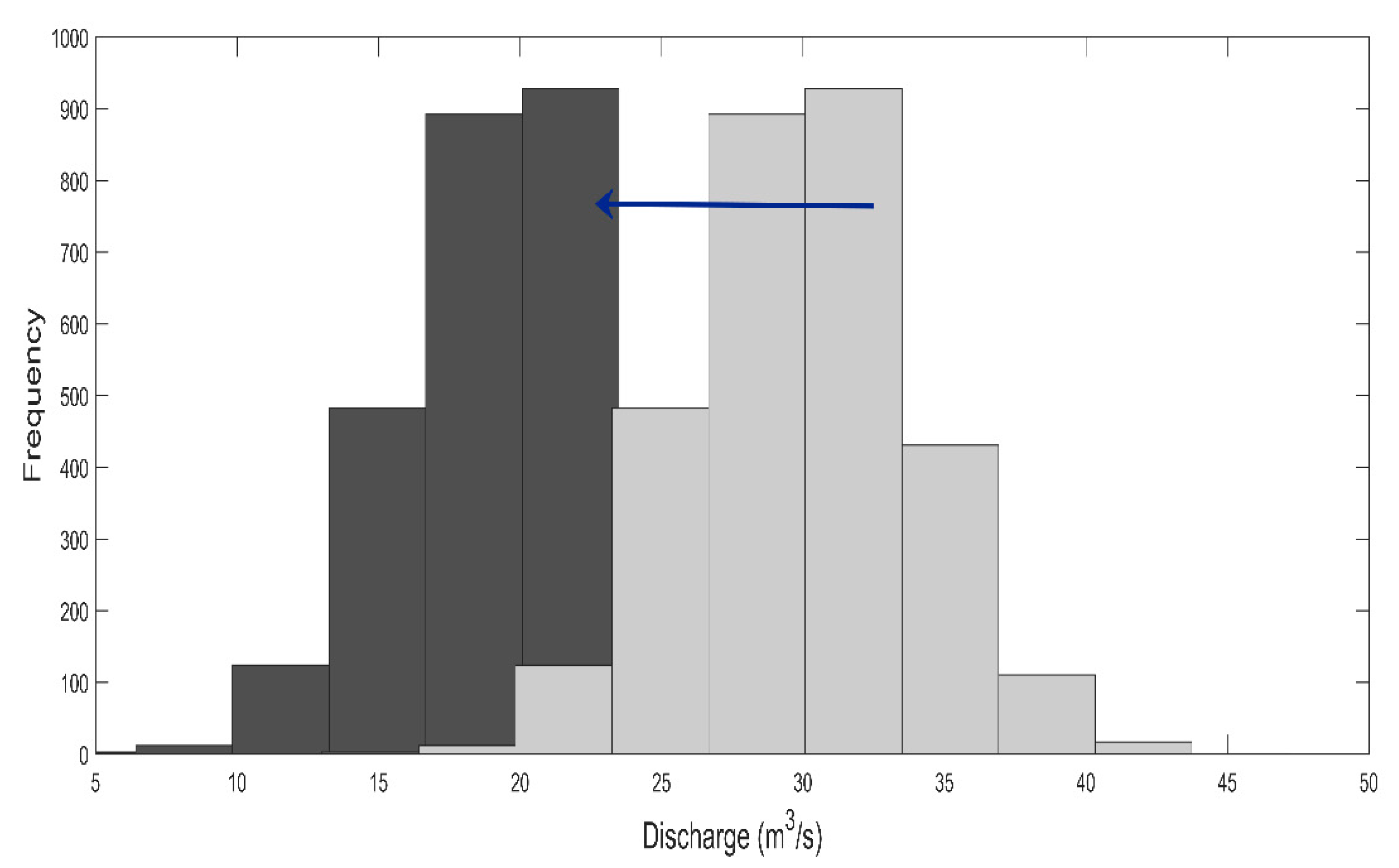
The former category of metrics (empirical, e.g., Q95, the 95th percentile of daily mean flows) is based on the following unstated assumptions: (1) past low-flow events allow for an adequate characterization of hydrological conditions to be encountered in the future; (2) the river ecosystem has evolved and adapted to the conditions that were prevalent historically and therefore is resilient to such conditions. The corollary to these assumptions is that a relatively extreme low flow, e.g., one that is exceeded 95% of the time historically, will likely occur and exceed just as often in the future, and the ecosystem will respond to this flow as it did in the past. Empirical frequencies are often summarized using histograms, such as the ones in Figure 1. In the context of climate change, the shape of the histogram will likely be altered in many ways. Firstly, the non-stationarity of order 1 may involve a trend or shift in the mean. In time, this can result in a full translation of the histogram of daily flows to the right (i.e., the average flow will increase) or the left (i.e., the average flow will decrease).
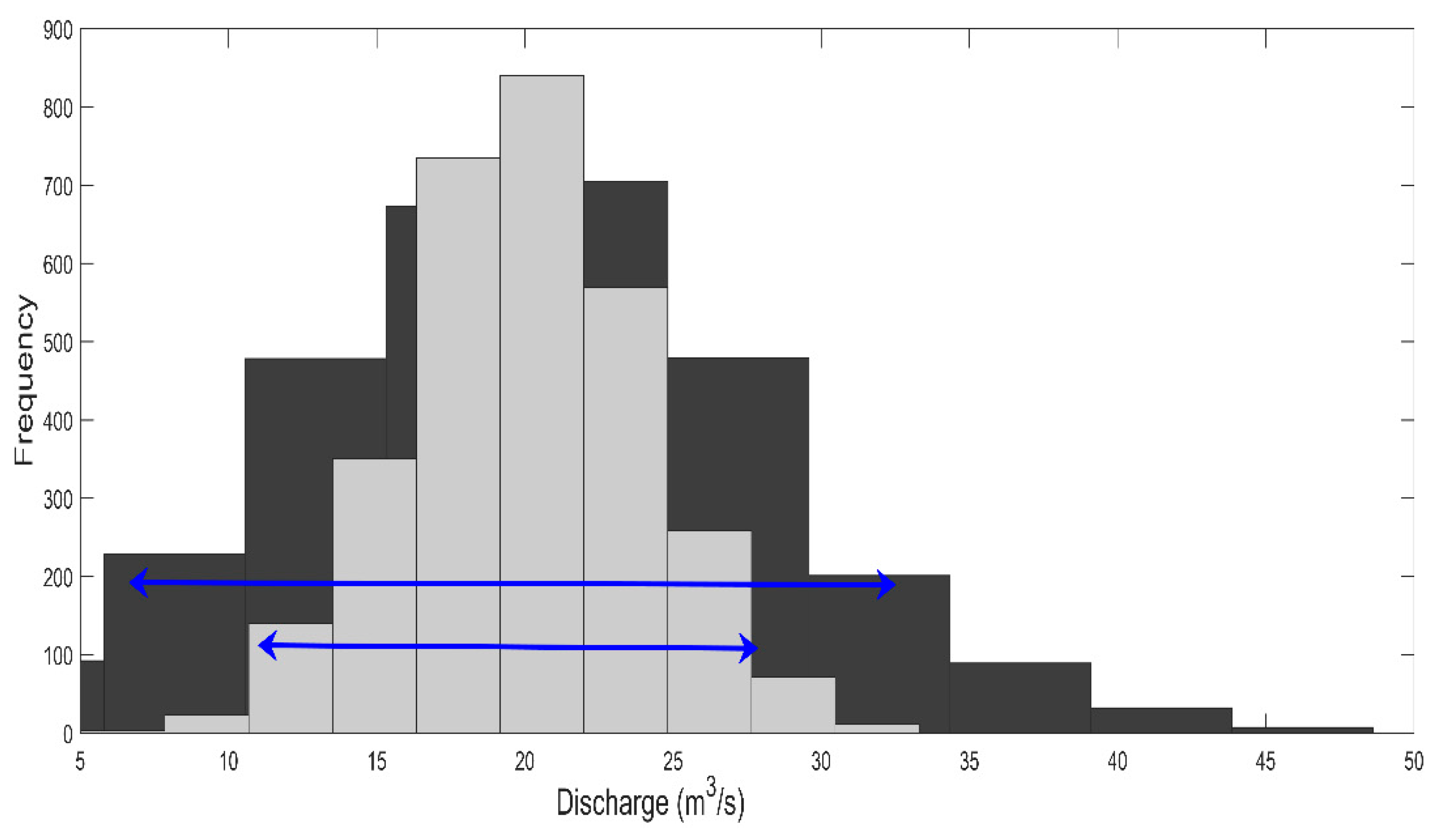
However, many authors indicate that the impact of climate change in many regions of the world may be a non-stationarity of order 2, i.e., an increase in variance. In this case, the histogram of daily flows in the future could be flattened, and its breadth increased compared to the historical time series (Figure 2). This flattening of the flow distribution implies that low-flow events would likely occur more frequently and that higher flows are likely as well (compared to those measured in the past). Hence, an eflow threshold metric, such as the Q95 (95th percentile) or the median flow (Q50) during low-flow months (e.g., August or September in mid-latitudes), will not occur at the same frequency in the future as in the past.
The non-stationarity of order 3 (i.e., a change in skewness) and order 4 (kurtosis) cannot be excluded but have been scantly explored in climate change studies. One potential reason for this exclusion was pointed out by Ulrych et al. [16], who stated that higher-order moments are more difficult to estimate than mean or variance. Their estimation can be more affected by the presence of outliers and small sample sizes than mean and variance estimators.
In some jurisdictions (e.g., the Quebec Department of Environment and Fight against Climate Change in Canada), the eflow metrics used for regulating water withdrawals and dissolving contaminants from effluents are based on low-flow frequency analysis. Unlike the aforementioned metrics, those based on frequency analysis are estimated using a parametric approach. Notably, the extremes (i.e., minimum flows) for a given duration (e.g., seven days) are extracted from the historical time series, and a statistical distribution F(x, θ) (where θ is the vector of parameters of the theoretical distribution) is fitted to these extremes. The theoretical probability of exceedance of the extremes (F) is estimated, and it can be related to the return period as shown in Equation (1) for low flows:
T(x): return period of a flow related to a given event x (years);
p: probability of exceedance, such as p = 1 − F(x, θ).
Classical frequency analysis is based on a number of assumptions, one of which is stationarity, i.e., the absence of a monotonic trend in the time series. Therefore, the approach appears ill-adapted in the context of climate change. Recent work on non-stationary frequency analysis has made it possible to change the constant parameters of the fitted statistical distribution to time-varying values, using covariates (see [17] for a review). This allows modelling the evolution of the parameters, and hence, the shape of the distribution over time. Two main challenges are associated with this approach in the context of eflows: (1) although non-stationary frameworks have been developed for a number of statistical distributions, it is incomplete, and the work has mostly focused on floods. (2) The concept of a return period has been historically defined in a stationary context and requires adaptations in a changing climate.
With regards to the first aforementioned challenge, the most commonly used frequency distributions in low-flow frequency analysis, according to Ouarda, Charron and St-Hilaire [18], are the Weibull, Gumbel, Log-Normal, Gamma, Pearson Type III and Log-Pearson Type III distributions. Other distributions have been used for low flows. For instance, Shao, Chen and Zhang [19] used the Burr III distribution, and Liu et al. [20] used the Generalized Extreme Value distribution. Hence, the selection of the distribution is often contextual and depends on the goodness of fit and parsimony, as well as the sample size, data quality and the quantiles of interest. Not all of these distributions have been tested on low-flow time series with trends, and much remains to be done (especially the development of time-varying parameter functions) before they can be fully applied in this context.
As for the second challenge, the concept of a return period in a stationary context is important for eflows prescription. T(x) is defined as the average period between events of a given magnitude. When T(x) becomes time-varying, i.e., T(x, t), this definition no longer holds. The return period is not fixed but rather changes over time. Time-varying low-flow quantiles may be puzzling and misleading for practitioners and regulatory bodies. For instance, if the trend is negative (i.e., decreasing over time), a two-year return period for a low-flow metric that is defined today will have a lower value in five or ten years. Alternatively, if the regulatory body states that the two-year return period is to be used, as currently defined, then this quantile will likely not have a return period of two years in a few decades.
Current methodologies lead practitioners to use a cascade of models to generate future hydrological scenarios, from which empirical or frequency analysis metrics related to the eflows can be calculated. Outputs from climate models, driven by more or less optimistic greenhouse gas emission scenarios (the so-called Representative Concentration Pathways or RCP), are used as inputs to hydrological models. When stationarity becomes a challenge in the analysis of the hydrological scenarios thus generated, it is often circumvented by breaking down the future time series in subsets of, e.g., 30 years for which stationarity can be assumed and/or validated by statistical tests. What is implied in this approach is that a (sometimes) monotonic trend over a long period (e.g., 100 years) is represented by shifts in the means between the shorter subsets. For regulatory bodies, this approach is easier to implement because the eflow regulation and the value(s) of the low-flow metric(s) used can be revisited at the onset of the new period (e.g., every 30 years). The practitioners can be comforted in the fact that the method used and perhaps even the criterion set by regulatory agencies may remain the same. However, should the more pessimistic climate change scenarios (e.g., RCP 8.5) become a reality, shifting the mean every 30 years may be insufficient to represent the true changes in low-flow regimes. Perhaps regulations that are based on statistical analyses need to be revisited and the period of analysis be prescribed and fixed to avoid the possibility that the practitioners chase a moving target. Any analysis that is based on climate change scenarios needs to be rooted in a probabilistic framework. An ensemble (i.e., multiple climate scenarios fed to multiple hydrological models) is often used to allow for probabilistic assessment. Bayesian approaches are often used to implement such frameworks (e.g., [21]).
3. Timing
The timing of low flows is of the utmost importance for aquatic fauna and flora. Species and communities have evolved to adapt to the occurrence of low-flow events, and in numerous instances, they are an environmental cue for shifts in behaviour, life history stage and/or function (e.g., [22]).
There is a large body of literature that focuses on possible shifts in low-flow timing in the hydrological year. Shift detection can perhaps be dependant to a certain degree on the statistical method used to detect them. This is beyond the scope of the present study. Within a large region or country, shifts or trends in timing can vary. In Canada, which is plagued with two low-flow seasons (winter and summer), the western part of the country is affected by low flows shifting toward later dates, while there is a trend for an earlier occurrence in most of the eastern part of the country [23]. This is corroborated by the analysis of climate change scenarios by Berthot et al. [24], who indicated that 195 stations in the Canadian province of Québec, representing 68% of all stations analyzed, will likely be characterized by earlier low flows in the summer than in the recent past or even a shift in seasonality, with winter low flows becoming less severe than summer low flows in many instances. Young et al. [25] studied the fate of low flows in the Sierra Nevada (California, USA) watersheds and expected that for every 10% decrease in the snowpack (as measured by peak snow water equivalent), annual minimum flows would likely decrease 9%–22% and their occurrence would be shifted 3–7 days earlier in the year. In the Eastern U.S., Sadri, Kam, and Sheffield [26] did not detect significant trends in the timing of low flows. In Iran, Dinpashoh et al. [27] studied 37 drainage basins and found negative slopes (i.e., a trend toward earlier occurrences) in time series of low-flow onset dates. The high variability in observed/modelled trends and shifts in the timing of low flows is a challenge for regulators. Given that the vast majority (70%) of water demand worldwide is from the agricultural sector (https://www.worldbank.org/en/topic/water-in-agriculture#:~:text=Currently%2C%20agriculture%20accounts%20(on%20average,to%20the%20evapotranspiration%20of%20crops; accessed on 30 March 2021), shifts in low-flow timings can potentially exacerbate the pressure on watersheds dominated by this activity.
Seasonal shifts (e.g., minimum flows occurring in the summer instead of the winter) must also be accounted for in the context of climate change. Some regulations are based on identifying the month of the year with the lowest flow (e.g., LQ50 in Table 1). In a study of the impact of climate change on the flow regimes in Europe, Arnell [28] indicated that the most significant changes are expected in the eastern part of the continent, where the snow water equivalent (SWE) will likely decrease and shift in part to liquid precipitation due to higher temperatures. This change will lead to winter runoff increases and spring flow decreases, which may, in turn, exacerbate summer low flows. In such regions, the historical time series of minima may overwhelmingly be composed of winter low flows, while future minima may be mostly occurring in the summer. Statistically, this may mean that current and future samples may be composed of realizations from two different populations. This poses an additional challenge for jurisdictions that are using frequency analysis to define eflow metrics (e.g., 7Q2, representing a mean low flow of 7 days with a 2-year return period) because the homogeneity of the sample (i.e., all realizations originate from the same population) is a requirement in frequency analysis.
Flow is not the only variable that is changing during the winter season. For many rivers, the ice-covered period is shortening or is predicted to become shorter than at present [29]. Future winter eflows prescriptions will need to account for possible longer ice-free periods in northern rivers.
4. Quality
Flow quantity is a quantitative concept that is relatively easy to grasp, whereas flow quality may be a term that is harder to define. Many authors have identified water quality as a key ecological service to be rendered by adequate eflow prescriptions. Water quality has different definitions according to usage (e.g., drinking water, agriculture, preservation of aquatic life, recreational activities, aesthetics and culture) and variables (temperature, turbidity, pH, dissolved solids, suspended sediments, etc.). In climate change studies, very few impact studies have managed to grasp the full spectrum of the links between expected flow variability (especially low flows) and water quality according to usage and indicator variables.
Some authors, such as Dahnya and Kumar [30], have argued for the inclusion of water quality in the definition of eflows, particularly in a changing climate. The model-cascade approach can be (and has been) applied to provide some water quality scenarios. Some examples include work that has focused on nutrients [31], on oxygen and biological oxygen demand [32], on organic carbon concentrations [33], etc. These models are of varying complexity, which may increase as a function of the complexity of the underlying chemical concepts that they attempt to predict.
One water quality variable that has been investigated at the global scale and for which scenarios of its possible evolution as a function of climate change have been generated is water temperature. For instance, Van Vliet et al. [34] linked an increase in the seasonality (or variance) of discharge (i.e., higher floods and lower low flows) anticipated for >30% of studied rivers worldwide to increases in mean and extreme river temperatures in the order of 1 to 2 °C. A number of local studies have also been completed to generate future river temperature scenarios (e.g., [35,36,37,38]). The main reasons for the relative popularity of water temperature studies related to climate change are (1) its ecological relevance: water temperature regulates metabolism, dictate in part species distribution, is an environmental cue for many migrating organisms and affects other biologically relevant water quality variables, such as dissolved oxygen. (2) Its relative simplicity: all stakeholders easily understand the implications of water warming or cooling. Additionally, water temperature is often well correlated with air temperature. The latter is arguably the most trustworthy climate model output. Hence, inference on and modelling of water temperature can be simpler than for other water quality variables. (3) Its ease of interpretation. While some water quality variables may be less amenable to public scrutiny, water temperature is a variable that is well understood by the general public, and especially by the angling community. (4) The relative abundance and ease of implementation of thermal models.
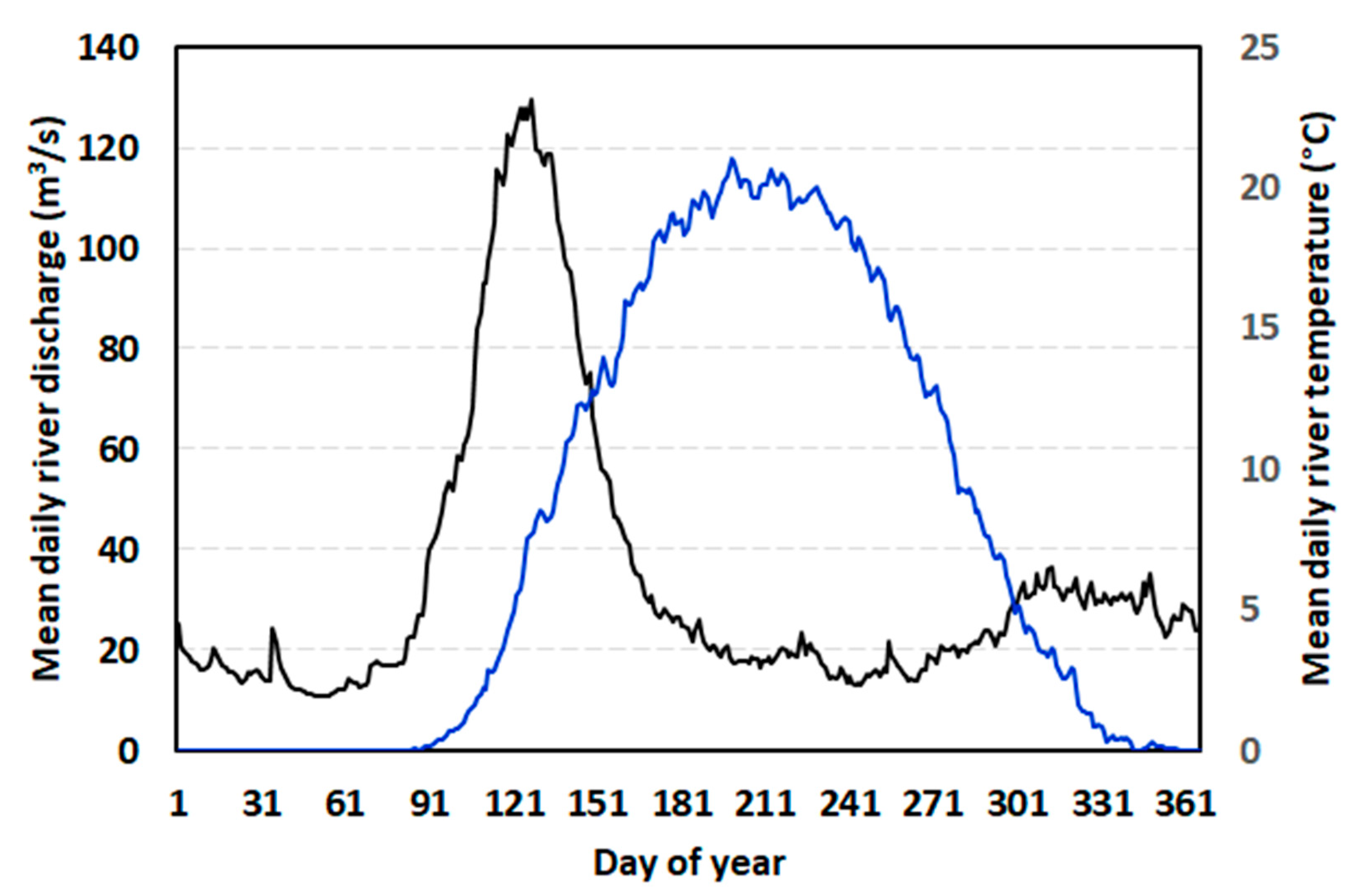
In spite of all these advantages, river temperature has scantly been used in eflow-related studies. Olden and Naiman [39] advocated for the inclusion of water temperature in eflow analyses, especially when they are performed to minimize the impacts of dam operations. They suggested that these thermal analyses should include a comprehensive characterization of seasonality and variability (both temporal and spatial) of river temperatures. It goes without saying that under constant radiative fluxes, a small volume of water associated with low flows will warm up faster than a larger volume of water associated with higher flows. However, as always, nature is not that simple. Rivers with similar flow regimes may have different thermal regimes. This thermal variability has many causes, including land use on the drainage basin, riparian vegetation, the relative contribution of groundwater to baseflow, etc. In recent years, the thermal classification of rivers has been a topic of research that has been gaining in popularity. The term “thermal sensitivity” (TS) has been used in the literature to compare different rivers. In its simplest form, TS has been defined as the slope of the regression between air temperature (Ta) and river temperature (Tw). The value of this slope provides a measure of the increase in Tw for, say, an increase in 1 °C of Ta [40], and streams and rivers can be classified according to this criterion. Other classifications have focused on the seasonality of the thermal regime. For instance, Maheu, Poff and St-Hilaire [41] used a simple sinusoidal curve fitted to interannual daily mean temperature time series to define six relatively homogenous groups of thermal regimes in the U.S. Daigle, Boyer and St-Hilaire [42] classified rivers in Québec (Canada) by using a similar approach but fitting a Gaussian function instead of a sine function to historical time series. These approaches can group rivers with similar thermal characteristics. Within these groups, eflows can be analyzed in the context of the impact of low flows on thermal variability as the first, simple approach to determine the combined role of anthropogenic exacerbation of low flows and temperature in the possible disturbance of ecological services and functions in riverine ecosystems [43]. Figure 3 shows an example of both flow and thermal regimes (long-term interannual averages) for the Little Southwest Miramichi River (New Brunswick, Canada), where the summer low flows are concurrent with high river temperatures. As such, eflow metrics need to take into account the river temperature regime during summer low flows.
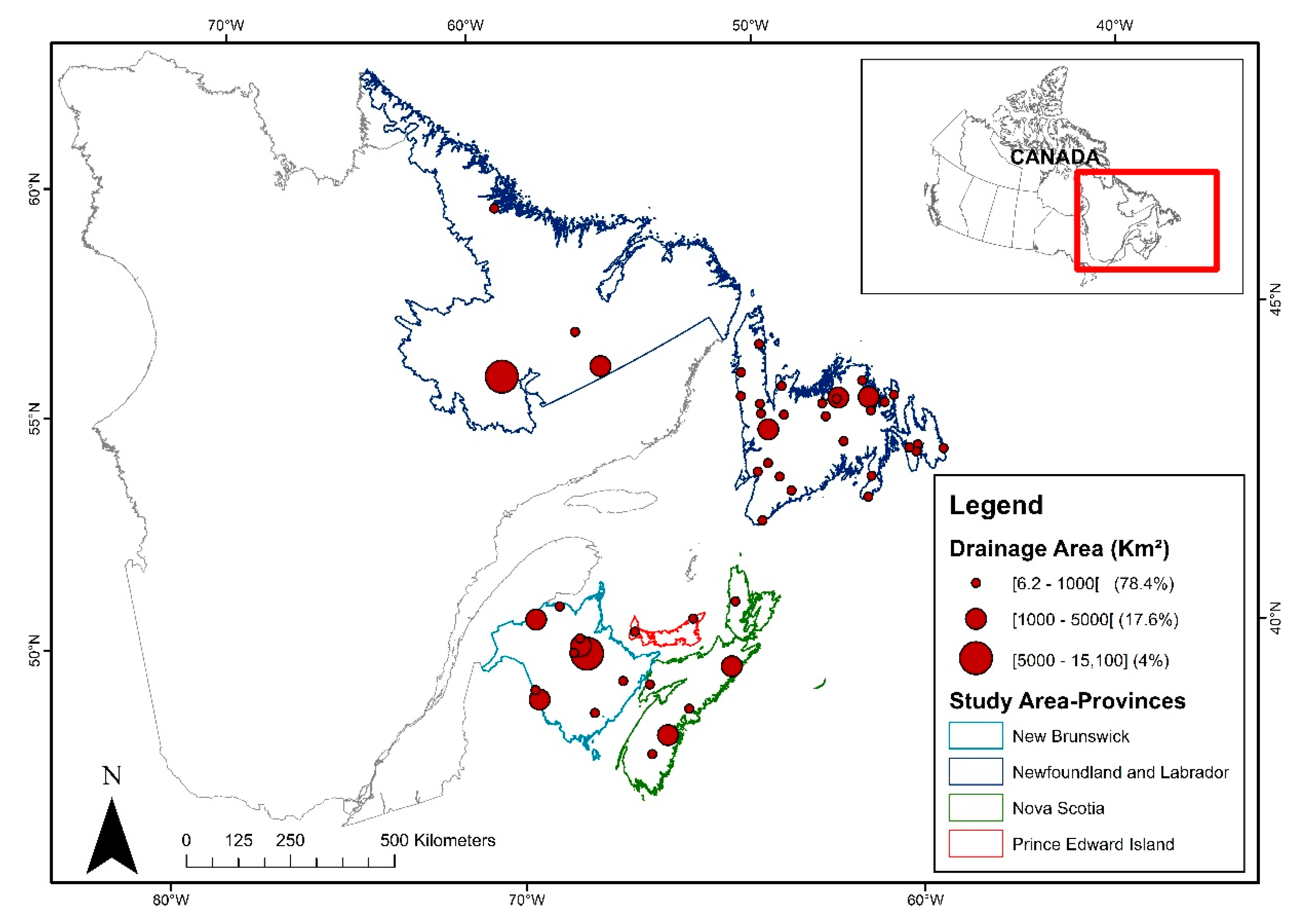
For instance, a recent study was conducted by our group in the Maritime Provinces of Eastern Canada, using 52 stations (Figure 4). Various hydrological eflow metrics were computed at all stations (Table 1), in addition to the percentages of MAF (Mean Annual Flow) thresholds. Then, maximum, minimum and mean temperatures associated with eflow metric occurrences (dates were selected with a tolerance of 15% around the value of the metrics) were analyzed from the associated water temperature time series.
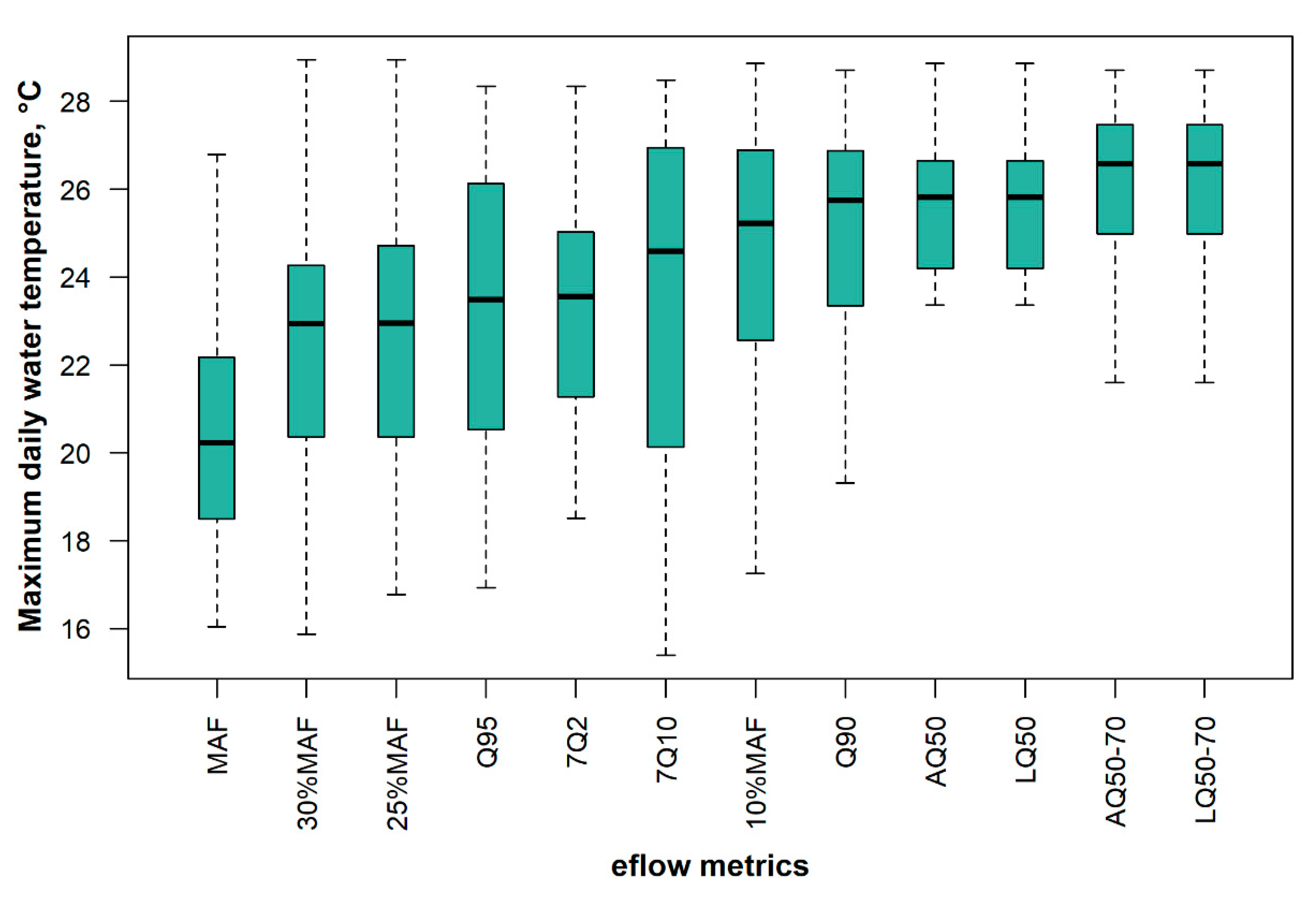
The results show that the interannual eflow metrics AQ50, AQ50-70, LQ50 and LQ50-70 are associated with the highest maximum river temperature during the summer (May–Sept) period in the majority of the stations across the different provinces. These eflows metrics also corresponded to the highest minimum and mean river temperature. In contrast, the 25%MAF, 30%MAF, Q90, Q95, 7Q2 and 7Q10 produced the highest variability of maximum river temperature in the majority of the stations, with similar results for the minimum and mean temperature. Figure 5 shows an example of maximum temperature variability in one of the hydrometric stations (01EF001) on the LaHave River in Nova Scotia (Canada). It clearly shows that AQ50 and AQ50-70 produce higher maximum water temperature and less variability than the rest of eflows because the associated events occurred in August, a warm summer month. For this station, the AQ50 and LQ50 are identical because August corresponds to the month with the lowest discharge.
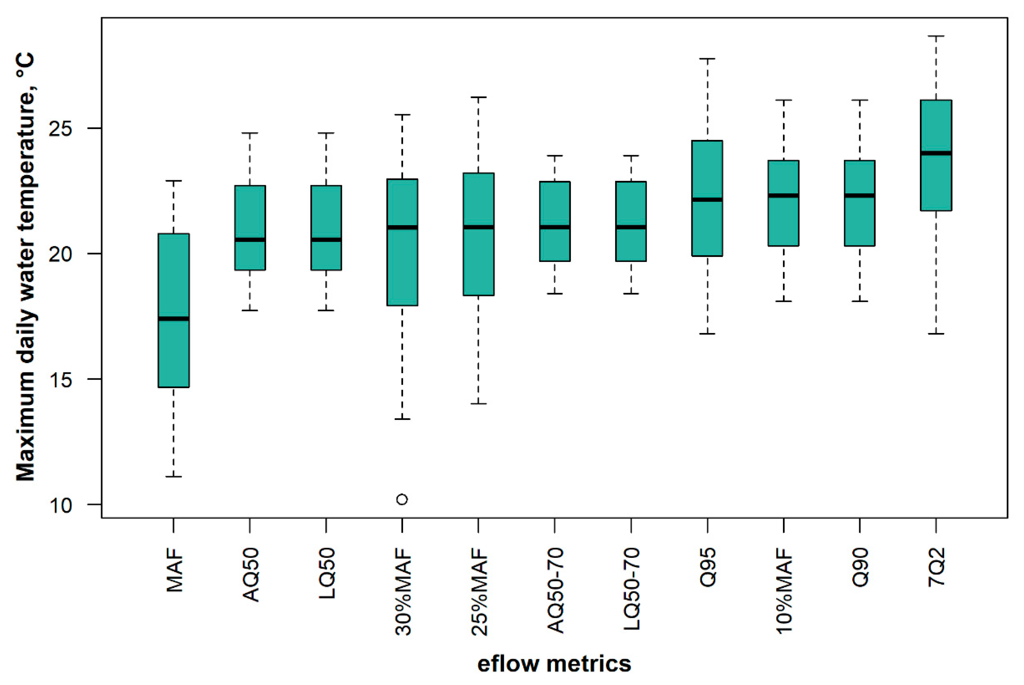
Among the 52 stations, the 7Q2 and 7Q10 resulted in the highest water temperature in 20% of the stations, mostly in the province of Newfoundland and Labrador (the largest island in Figure 4). Figure 6 shows the boxplot of maximum river temperature associated with each eflow for the Southern Bay River in the province of Newfoundland and Labrador. It is clear the 7Q2 results in higher temperature than the rest of the eflows metrics. This is caused by the fact that at that station, minimum flows occur in the summer. Metrics based on percentages of Mean Annual Flows show more variability because they are typically occurring throughout the ice-free season and can be associated with cooler or warmer periods. Again, AQ50 and LQ50 are identical.
The examples in Figure 5 and Figure 6 are likely representative of thermal patterns for rivers in mid to high latitudes. However, regions for which there is scant information are those with permafrost rivers. Makarieva et al. [44] indicated that processes causing changes for basins where permafrost remains dominant are poorly understood. In addition, they stated that small- and medium-sized permafrost river basins have been neglected in the literature.
5. Holistic Approaches
While hydrologic-based eflow methods remain popular, many jurisdictions are turning to more holistic approaches (e.g., [45,46]). The foundation for this movement was laid many decades ago with the advent of the Instream Flow Incremental Methodology (IFIM; [47]) and gained in popularity with the publication of the Ecological Limits of Hydrological Alteration (ELOHA) framework ([48]; Figure 7), which was a more generalized attempt to specifically include components of the hydrograph other than low flows and flow-ecology relationships in the decision-making process. In the original ELOHA (coloured boxes in Figure 7), the first step is developing the so-called hydrological foundation (which includes archived data retrieval and analysis, as well as hydrological modelling). Step 2 deals with grouping rivers with similar hydro geomorphological attributes. Step 3 involves analyzing the flow attributes in control and impacted environments to measure changes in flow amplitude, duration, timing, variability and frequency of events [49]. Step 4 is where flow-ecology relationships are defined, and hypotheses on the impact of altered flow on ecological functions are constructed. These steps inform stakeholders and/or regulatory agencies who are ultimately responsible for the decision and implementation of an eflow regime.
This formal framework was preceded by a plethora of ad hoc implementations of habitat models to address local eflow issues (e.g., [50]), which remain popular to this day (e.g., [51]). Habitat modelling is one of the methods to investigate and infer flow-ecology relationships (ELOHA step 4). There are many critics that have highlighted the limits of habitat models in eflow assessments. These criticisms include: (1) They tend to be monospecific or guild-focused; (2) their application is often spatially limited; (3) they do not necessarily account for the required connectivity between habitats; (4) they are most frequently not calibrated/validated for extreme conditions; (5) habitat availability and suitability is not necessarily akin to habitat use and not necessarily related to the productive capacity of rivers. In general, these models need more validation in order to become better predictive tools.
Nevertheless, habitat models remain useful and are used in local applications but will have to be adapted, given the plasticity of certain species and their potential shifts in habitats/territory. In northern regions, the vast majority of habitat model applications are for the ice-free season. Winter habitat may be more restrictive, and it could be argued that a more astute approach to eflow determination would be to investigate flow–habitat relationships outside of the fair-weather period.
In the ELOHA framework, flow-ecology relationships are not necessarily defined by habitat models. Other approaches, such as expert advice and uptake of traditional knowledge, empirical/statistical relationships based on field observations and/or meta-analyses, etc., can be implemented. With climate changes, some of these methods, i.e., those that are strictly based on past experiences, may be limited in scope.
In Figure 7, we argue for the inclusion of basic additional steps in the ELOHA framework (white boxes). First, the inclusion of river temperature as an element of classification will complement the hydrogeo-morphological classification proposed in the original framework and lead to a more ecologically relevant grouping of rivers. Secondly, hydro-climate change scenarios need to be included in eflow analyses. Climate change scenarios, in conjunction with possible changes in the ecological conditions (e.g., shifts in species territories, the timing of migrations, change in growth rates, etc.), will need to be considered in step 4 of the ELOHA framework.
6. Conclusions
This overview of possible challenges associated with eflow determination in the context of climate change emphasizes the fact that classical methods, especially hydrological methods, will require adaptations. The simplest form of adaptation would be to ask that metrics be calculated on the historical data that preceded the non-stationarity, provided that this stationary historical time series is sufficiently long to encapsulate the natural variability of the system under study, which can prove to be an important limiting factor. In most parts of the world, summer low-flow metrics thus calculated would likely be more conservative than those computed from synthetic flow time series obtained using the climate-hydrological model cascades.
A number of additional factors could, however, be taken into account to fully abide by the definition of eflows quoted herein, i.e., a definition that includes timing and quality of flows. Shifts in the seasonality of occurrence of minimum flows should be accounted for, especially in northern latitudes. As for quality, the inclusion of at least one relatively simple additional water quality variable, namely temperature, would be a step forward and one that would assist regulators and practitioners in providing a fuller assessment of the impact of the changing climate on the aquatic ecosystems. Although the case study presented in this paper may not be representative of all river ecosystems, it exemplifies how this additional variable may be of great assistance to select an appropriate eflow hydrological metric.
Finally, holistic approaches appear to be better suited for a thorough assessment of instream flow needs and environmental flows prescriptions. Simple modifications to the ELOHA framework were proposed to formalize non-stationarity in the process.
Author Contributions
A.S.-H. is the lead author and contributed most to the text, with the assistance of L.B., H.F. and D.C. In addition, D.C. contributed to the analysis that helped produced Figure 3. L.B. completed all of the analyses in the province of Québec, while H.F. produced all of the analyses in Atlantic Canada, except for Figure 3. All authors have read and agreed to the published version of the manuscript.
Funding
This research was funded in part by the Québec Department of Environment and Fight against Climate Change and Fisheries and Oceans Canada.
Institutional Review Board Statement
There is no humun or animal involved.
Data Availability Statement
Temperature data used for the Atlantic Provinces originate from the RivTemp database (www.rivtemp.ca, accessed on 12 April 2021) or DataStream. Flows were provided by the HYDAT database. Flows and temperatures in Québec were provided by the Québec Department of Environment and Fight against Climate Change.
Conflicts of Interest
The authors declare no conflict of interest.
References
- The Brisbane Declaration. Environmental Flows Are Essential for Freshwater Ecosystem Health and Human Well-Being. In Proceedings of the 10th International River Symposium and International Environmental Flows Conference, Brisbane, Australia. 2007. Available online: https://www.conservationgateway.org/ConservationPractices/Freshwater/EnvironmentalFlows/MethodsandTools/ELOHA/Pages/Brisbane-Declaration.aspx (accessed on 30 March 2021).
- Arthington, A.H.; Bhaduri, A.; Bunn, S.E.; Jackson, S.E.; Tharme, R.E.; Tickner, D.; Young, B.; Acreman, M.; Baker, N.; Capon, S.; et al. The Brisbane Declaration and Global Action Agenda on Environmental Flows (2018). Front. Environ. Sci. 2018, 6, 45. [Google Scholar] [CrossRef] [Green Version]
- Acreman, M.; Arthington, A.H.; Colloff, M.J.; Couch, C.; Crossman, N.D.; Dyer, F.; Overton, I.; Pollino, C.A.; Stewardson, M.J.; Young, W. Environmental flows for natural, hybrid, and novel riverine ecosystems in a changing world. Front. Ecol. Environ. 2014, 12, 466–473. [Google Scholar] [CrossRef] [Green Version]
- Davies, P.M.; Naiman, R.J.; Warfe, D.M.; Pettit, N.E.; Arthington, A.H.; Bunn, S.E. Flow–ecology relationships: Closing the loop on effective environmental flows. Mar. Freshw. Res. 2014, 65, 133–141. [Google Scholar] [CrossRef]
- Arthington, A.H.; Zalucki, J.M. The Land and Water Resources Research and Development Corporation (Australia). In Comparative Evaluation of Environmental Flow Assessment Techniques: Review of Methods; ACT, Land and Water Resources Research and Development Corp: Canberra, Australia, 1998. Available online: http://lwa.gov.au/files/products/river-landscapes/pr980305/pr980305.pdf (accessed on 30 March 2021).
- Leroy, T.D. Instream Flow Regimens for Fish, Wildlife, Recreation and Related Environmental Resources. Fisheries 1976, 1, 6–10. [Google Scholar]
- Tharme, R.E. A global perspective on environmental flow assessment: Emerging trends in the development and application of environmental flow methodologies for rivers. River Res. Appl. 2003, 19, 397–441. [Google Scholar] [CrossRef]
- Acreman, M.; Overton, I.; King, J.; Wood, P.J.; Cowx, I.; Dunbar, M.J.; Kendy, E.; Young, W. The changing role of ecohydrological science in guiding environmental flows. Hydrol. Sci. J. 2014, 59, 433–450. [Google Scholar] [CrossRef]
- Acreman, M.C.; Ferguson, A.J.D. Environmental flows and the European Water Framework Directive. Freshw. Biol. 2010, 55, 32–48. [Google Scholar] [CrossRef]
- Caissie, D.; El-Jabi, N.; Hébert, C. Comparison of hydrologically based instream flow methods using a resampling technique. Can. J. Civ. Eng. 2007, 34, 66–74. [Google Scholar] [CrossRef]
- MELCC. Calcul et Interprétation des Objectifs Environnementaux de Rejet Pour les Contaminants du Milieu Aquatique, 2nd ed.; Ministère du Développement Durable, de l’Environnement et des Parcs, Direction du Suivi de l’état de l’Environnement: Montreal, QC, Canada, 2007; 56p, ISBN 978-2-550-49172-9.
- Linnansaari, T.; Monk, W.A.; Baird, D.J.; Curry, R.A. Review of Approaches and Methods to Assess Environmental Flows across Canada and Internationally; Document 2012/039, DFO Canadian Sciences Advisory Secretary Research; DFO: Ottawa, ON, Canada, 2012.
- MELCC. Direction de l’Expertise Hydrique et Atmosphérique du Québec. In Guide de Conception des Installations de Production d’eau Potable; MELCC: Quebec City, QC, Canada, 2015; Volume 1. Available online: http://www.environnement.gouv.qc.ca/eau/potable/guide/index.htm (accessed on 29 January 2021).
- USFWS (United States Fish and Wildlife Service). Interim Regional Policy for New England Streams Flow Recommendations; Memorandum from H.N. Larsen: Newton Corner, MA, USA, 1981. [Google Scholar]
- Caissie, D.; Eljabi, N. Hydrologically Based Environmental Flow Methods Applied to Rivers in the Maritime Provinces (Canada). River Res. Appl. 2015, 31, 651–662. [Google Scholar] [CrossRef]
- Ulrych, T.J.; Velis, D.R.; Woodbury, A.D.; Sacchi, M.D. L-moments and C-moments. Stoch. Environ. Res. Risk Assess. 2000, 14, 50–68. [Google Scholar] [CrossRef]
- Khaliq, M.; Ouarda, T.; Ondo, J.-C.; Gachon, P.; Bobée, B. Frequency analysis of a sequence of dependent and/or non-stationary hydro-meteorological observations: A review. J. Hydrol. 2006, 329, 534–552. [Google Scholar] [CrossRef]
- Ouarda, T.B.; Charron, C.; St-Hilaire, A. Statistical Models and the Estimation of Low Flows. Can. Water Resour. J. 2008, 33, 195–206. [Google Scholar] [CrossRef] [Green Version]
- Shao, Q.; Chen, Y.D.; Zhang, L. An extension of three-parameter Burr III distribution for low-flow frequency analysis. Comput. Stat. Data Anal. 2008, 52, 1304–1314. [Google Scholar] [CrossRef]
- Liu, D.; Guo, S.; Lian, Y.; Xiong, L.; Chen, X. Climate-informed low-flow frequency analysis using nonstationary modelling. Hydrol. Process. 2014, 29, 2112–2124. [Google Scholar] [CrossRef]
- Najafi, M.R.; Moradkhani, H. A hierarchical Bayesian approach for the analysis of climate change impact on runoff extremes. Hydrol. Process. 2013, 28, 6292–6308. [Google Scholar] [CrossRef]
- Tornabene, B.J.; Smith, T.W.; Tews, A.E.; Beattie, R.P.; Gardner, W.M.; Eby, L.A. Trends in River Discharge and Water Temperature Cue Spawning Movements of Blue Sucker, Cycleptus elongatus, in an Impounded Great Plains River. Copeia 2020, 108, 151. [Google Scholar] [CrossRef] [Green Version]
- Ehsanzadeh, E.; Adamowski, K. Trends in timing of low stream flows in Canada: Impact of autocorrelation and long-term persistence. Hydrol. Process. 2010, 24, 970–980. [Google Scholar] [CrossRef]
- Berthot, L. Comparaison des Méthodes D’estimation des Débits Environnementaux au Québec, dans un Contexte Hydrologique et Climatique Actuel et Futur; Report Submitted to the Quebec Department of Environment and Climate Change; # 2032; INRS: Quebec City, QC, Canada, 2010; 37p. [Google Scholar]
- Young, C.A.; Escobar-Arias, M.I.; Fernandes, M.; Joyce, B.; Kiparsky, M.; Mount, J.F.; Mehta, V.K.; Purkey, D.; Viers, J.H.; Yates, D. Modeling the Hydrology of Climate Change in California’s Sierra Nevada for Subwatershed Scale Adaptation1. JAWRA J. Am. Water Resour. Assoc. 2009, 45, 1409–1423. [Google Scholar] [CrossRef]
- Sadri, S.; Kam, J.; Sheffield, J. Nonstationarity of low flows and their timing in the eastern United States. Hydrol. Earth Syst. Sci. 2016, 20, 633–649. [Google Scholar] [CrossRef] [Green Version]
- Dinpashoh, Y.; Singh, V.P.; Biazar, S.M.; Kavehkar, S. Impact of climate change on streamflow timing (case study: Guilan Province). Theor. Appl. Clim. 2019, 138, 65–76. [Google Scholar] [CrossRef]
- Arnell, N.W. The effect of climate change on hydrological regimes in Europe: A continental perspective. Glob. Environ. Chang. 1999, 9, 5–23. [Google Scholar] [CrossRef]
- Magnuson, J.J.; Robertson, D.M.; Benson, B.J.; Wynne, R.H.; Livingstone, D.M.; Arai, T.; Assel, R.A.; Barry, R.G.; Card, V.; Kuusisto, E.; et al. Historical Trends in Lake and River Ice Cover in the Northern Hemisphere. Science 2000, 289, 1743–1746. [Google Scholar] [CrossRef] [PubMed] [Green Version]
- Dahnya, C.T.; Kumar, A. Making a Case for Estimating Environmental Flow under Climate Change. Curr. Sci. 2015, 109, 1019–1020. [Google Scholar]
- Arheimer, B.; Andréasson, J.; Fogelberg, S.; Johnsson, H. Climate Change Impact on Water Quality: Model Results from Southern Sweden. Ambio 2005, 34, 559–566. [Google Scholar] [CrossRef] [PubMed]
- Mimikou, M.; Baltas, E.; Varanou, E.; Pantazis, K. Regional impacts of climate change on water resources quantity and quality indicators. J. Hydrol. 2000, 234, 95–109. [Google Scholar] [CrossRef]
- Whitehead, P.G.; Wilby, R.L.; Battarbee, R.W.; Kernan, M.; Wade, A.J. A review of the potential impacts of climate change on surface water quality. Hydrol. Sci. J. 2009, 54, 101–123. [Google Scholar] [CrossRef]
- Van Vliet, M.T.H.; Wietse, H.P.F.; Yearsley, J.R.; Ludwig, F.; Haddeland, I.; Lettenmaier, D.P.; Kabat, P. Global River Discharge and Water Temperature under Climate Change. Glob. Environ. Chang. 2013, 23, 450–464. [Google Scholar] [CrossRef]
- Islam, S.U.; Hay, R.W.; Déry, S.J.; Booth, B.P. Modelling the impacts of climate change on riverine thermal regimes in western Canada’s largest Pacific watershed. Sci. Rep. 2019, 9, 1–14. [Google Scholar] [CrossRef] [PubMed]
- Daigle, A.; Jeong, D.I.; Lapointe, M.F. Climate change and resilience of tributary thermal refugia for salmonids in eastern Canadian rivers. Hydrol. Sci. J. 2015, 60, 1044–1063. [Google Scholar] [CrossRef]
- Arismendi, I.; Safeeq, M.; Dunham, J.B.; Johnson, S.L. Can air temperature be used to project influences of climate change on stream temperature? Environ. Res. Lett. 2014, 9, 084015. [Google Scholar] [CrossRef]
- Chang, H.; Psaris, M. Local landscape predictors of maximum stream temperature and thermal sensitivity in the Columbia River Basin, USA. Sci. Total. Environ. 2013, 461–462, 587–600. [Google Scholar] [CrossRef]
- Olden, J.D.; Naiman, R.J. Incorporating thermal regimes into environmental flows assessments: Modifying dam operations to restore freshwater ecosystem integrity. Freshw. Biol. 2010, 55, 86–107. [Google Scholar] [CrossRef]
- Kelleher, C.; Wagener, T.; Gooseff, M.N.; McGlynn, B.L.; McGuire, K.; Marshall, L. Investigating controls on the thermal sensitivity of Pennsylvania streams. Hydrol. Process. 2011, 26, 771–785. [Google Scholar] [CrossRef]
- Maheu, A.; Poff, N.L.; St-Hilaire, A. A Classification of Stream Water Temperature Regimes in the Conterminous USA. River Res. Appl. 2015, 32, 896–906. [Google Scholar] [CrossRef]
- Daigle, A.; Boyer, C.; St-Hilaire, A. A standardized characterization of river thermal regimes in Québec (Canada). J. Hydrol. 2019, 577, 123963. [Google Scholar] [CrossRef]
- Wei, S.; Zhao, J.; Tong, X. Impacts of socio-economic status and environmental attitudes of locals on E-flow allocation in Weihe River Basin, China. HydroResearch 2020, 3, 158–165. [Google Scholar] [CrossRef]
- Makarieva, O.; Nesterova, N.; Post, D.A.; Sherstyukov, A.; Lebedeva, L. Warming temperatures are impacting the hydrometeorological regime of Russian rivers in the zone of continuous permafrost. Cryosphere 2019, 13, 1635–1659. [Google Scholar] [CrossRef] [Green Version]
- O’Brien, G.C.; Dickens, C.; Hines, E.; Wepener, V.; Stassen, R.; Quayle, L.; Fouchy, K.; MacKenzie, J.; Graham, P.M.; Landis, W.G. A regional-scale ecological risk framework for environmental flow evaluations. Hydrol. Earth Syst. Sci. 2018, 22, 957–975. [Google Scholar] [CrossRef] [Green Version]
- Bovee, K. A Guide to Stream Habitat Analysis Using the Instream Flow Incremental Methodology; USDI, Information Paper; Fish and Wildlife Service, Office of the Biological Services: Fort Collins, CO, USA, 1982; Volume 12.
- Poff, N.L.; Richter, B.D.; Arthington, A.H.; Bunn, S.E.; Naiman, R.J.; Kendy, E.; Acreman, M.; Apse, C.; Bledsoe, B.P.; Freeman, M.C.; et al. The ecological limits of hydrologic alteration (ELOHA): A new framework for developing regional environmental flow standards. Freshw. Biol. 2010, 55, 147–170. [Google Scholar] [CrossRef] [Green Version]
- Poff, N.L.; Allan, J.D.; Bain, M.B.; Karr, J.R.; Prestegaard, K.L.; Richter, B.D.; Sparks, R.E.; Stromberg, J.C. The Natural Flow Regime. Bioscience 1997, 47, 769–784. [Google Scholar] [CrossRef]
- Leclerc, M.; Saint-Hilaire, A.; Bechara, J. State-of-the-Art and Perspectives of Habitat Modelling for Determining Conservation Flows. Can. Water Resour. J. 2003, 28, 135–151. [Google Scholar] [CrossRef]
- Hough, I.M.; Warren, P.H.; Shucksmith, J.D. Designing an Environmental Flow Framework for Impounded River Systems through Modelling of Invertebrate Habitat Quality. Ecol. Indic. 2019, 106, 105445. [Google Scholar] [CrossRef]
- Park, S.-Y.; Sur, C.; Lee, J.-H.; Kim, J.-S. Ecological drought monitoring through fish habitat-based flow assessment in the Gam river basin of Korea. Ecol. Indic. 2020, 109, 105830. [Google Scholar] [CrossRef]
Figure 1.
Histograms of daily flows with a mean of 20 m3/s (light colour) and a mean of 30 m3/s (dark colour). Both series have the same variance.
Figure 1.
Histograms of daily flows with a mean of 20 m3/s (light colour) and a mean of 30 m3/s (dark colour). Both series have the same variance.

Figure 2.
Histograms of daily flows with the same mean of 20 m3/s and a standard deviation of 4 m3/s (dark colour) and 3 m3/s (light colour).
Figure 2.
Histograms of daily flows with the same mean of 20 m3/s and a standard deviation of 4 m3/s (dark colour) and 3 m3/s (light colour).

Figure 3.
Interannual daily mean flow (black: 1952–2019) and river temperature (blue: 1992–2016) regimes for the Little Southwest Miramichi River, showing the low-flow and high-temperature periods.
Figure 3.
Interannual daily mean flow (black: 1952–2019) and river temperature (blue: 1992–2016) regimes for the Little Southwest Miramichi River, showing the low-flow and high-temperature periods.

Figure 4.
Location of hydrometric stations in the Maritime Provinces.

Figure 5.
Boxplot of the maximum daily water temperatures (°C) associated with eflow metrics for the LaHave River in Nova Scotia.
Figure 5.
Boxplot of the maximum daily water temperatures (°C) associated with eflow metrics for the LaHave River in Nova Scotia.

Figure 6.
Boxplot of the maximum daily water temperatures (°C) associated with eflows for the Southern Bay River in Newfoundland and Labrador.
Figure 6.
Boxplot of the maximum daily water temperatures (°C) associated with eflows for the Southern Bay River in Newfoundland and Labrador.

Figure 7.
Adaptation of the Ecological Limits of Hydrological Alteration (ELOHA) framework to a changing climate (original ELOHA figure from [38]).
Figure 7.
Adaptation of the Ecological Limits of Hydrological Alteration (ELOHA) framework to a changing climate (original ELOHA figure from [38]).


Table 1.
Environmental flow metrics, definitions and uses.
| Hydrological Metric Used for Eflows Determination | Symbol | Jurisdiction | Reference |
|---|---|---|---|
| 95th percentile on the flow duration curve | Q95 | United Kingdom | [9] |
| 90th percentile on the flow duration curve | Q90 | Tested in New Brunswick (Canada) | [10] |
| Mean 7-day low flow with a return period of two years | 7Q2 | Southern Quebec | [11] |
| Mean 7-day low flow with a return period of ten years | 7Q10 | United States | [12] |
| Quebec | [13] | ||
| Mean 30-day low flow with a return period of five years | 5Q30 | Southern Quebec | [13] |
| Median monthly flow of August | AQ50 | New England (also called Aquatic Base Flow) | [14] |
| 25% of the mean annual flow | 25%MAF | Nova Scotia | [12] |
| 70% of the median monthly flow of August | AQ50-70 | Prince Edward Island | [15] |
| Median discharge value of the month with lowest flows | LQ50 | Tested in New Brunswick (Canada) | [15] |
| 70% of the median of the month with lowest flows | LQ50-70 | Tested in New Brunswick (Canada) | [15] |
Publisher’s Note: MDPI stays neutral with regard to jurisdictional claims in published maps and institutional affiliations. |
© 2021 by the authors. Licensee MDPI, Basel, Switzerland. This article is an open access article distributed under the terms and conditions of the Creative Commons Attribution (CC BY) license (https://creativecommons.org/licenses/by/4.0/).
Share and Cite
MDPI and ACS Style
St-Hilaire, A.; Ferchichi, H.; Berthot, L.; Caissie, D. The Fate of Stationary Tools for Environmental Flow Determination in a Context of Climate Change. Water 2021, 13, 1203. https://doi.org/10.3390/w13091203
AMA Style
St-Hilaire A, Ferchichi H, Berthot L, Caissie D. The Fate of Stationary Tools for Environmental Flow Determination in a Context of Climate Change. Water. 2021; 13(9):1203. https://doi.org/10.3390/w13091203
Chicago/Turabian StyleSt-Hilaire, André, Habiba Ferchichi, Laureline Berthot, and Daniel Caissie. 2021. "The Fate of Stationary Tools for Environmental Flow Determination in a Context of Climate Change" Water 13, no. 9: 1203. https://doi.org/10.3390/w13091203
Note that from the first issue of 2016, this journal uses article numbers instead of page numbers. See further details here.