1. Introduction
SWP can be measured directly in field by means of different sensors, such as tensiometers, heat dissipation sensors and dielectric sensors [
1,
2,
3,
4,
5,
6,
7,
8,
9]. Furthermore, the measures can be carried out also in a laboratory on soil samples and also through thermocouple psychrometry, dew point potential meters or filter paper techniques [
10]. Measurements of SWP carried out through these devices give precise assessment of hydrological properties, such as Soil Water Characteristic Curves (SWCCs) and Hydraulic Conductivity Functions (HCFs), and of hydrological behaviors, even if they are usually expensive and limited to few samples representative of small study areas, disregarding the possible variations of this parameter at wider scales [
11].
To enlarge the assessment of SWP in time and in space, deterministic models can be implemented. In the frame of this approach, volume balance models [
12,
13,
14] apply empirical equations, allowing one to estimate SWP dynamics from the meteorological (e.g., rainfall, air temperature) and the soil water balance (e.g., runoff, evapotranspiration) parameters. Instead, dynamic numerical models assess SWP dynamics and behaviors solving water flows in soil, on the basis of the parameters of water balance and the main soil hydrological properties, represented by SWCCs and HCFs [
5,
15,
16]. Even if these models estimate spatio-temporal SWP dynamics through robust physically-based processes, they can be limited by the availability of soil properties that are difficult to collect over large areas and by the effective preliminary calibration of the hydrological parameters used in the models [
17,
18].
Data-driven methods based on multiple regression analyses, time series methods or machine learning have been proposed since the 2000s to overcome the limitation of physically-based methodologies for the spatial and temporal assessment of some soil hydrological properties, namely soil-water contents [
19,
20,
21,
22,
23,
24] and groundwater levels [
25,
26,
27,
28]. Since the model coefficients of multiple regression analyses are affected by spatio-temporal distribution and the time series method has some limitations on medium and long-term predictions, data-driven models for soil moisture or groundwater level assessment are generally built on machine learning techniques, mostly Artificial Neural Networks, Support Vector Machines, Random Forests [
29].
Although these methodologies generally guarantee a high predictive capability of temporal trends [
22], they have not been applied for the assessment of SWP dynamics yet. The main constraint on modeling this parameter is the wide range of fluctuation along time, since SWP could change typically in field from positive or nil values in saturated conditions to −10
3/−10
2 m of water column in dry conditions of fine materials [
30]. Moreover, another constraint is related to a correct modeling of the transient state when SWP passes from negative (unsaturated) to nil or positive (saturated) conditions. These situations occur during intense rainfall events and represent the typical triggering conditions of shallow landslides that affect generally the soil horizons in the first 2 m in depth [
7,
31].
In order to fill this gap, this paper aims to develop and validate a machine learning methodology able to assess correctly the temporal dynamics of SWP at different depths and for soils with different physical, geotechnical and hydrological features. In order to reach this goal, the following objectives were considered: (i) selecting the best machine learning technique able to estimate the temporal trends of SWP acquired in field at different depths in test-sites with different soil features; (ii) evaluating the effects of the different predictors on the performance of the models; (iii) investigating the possibility of using the modeled SWP data to assess the safety factor of a slope and to select the most appropriate rainfall threshold in order to identify shallow landslides triggering times.
2. Materials and Methods
2.1. Test-Sites
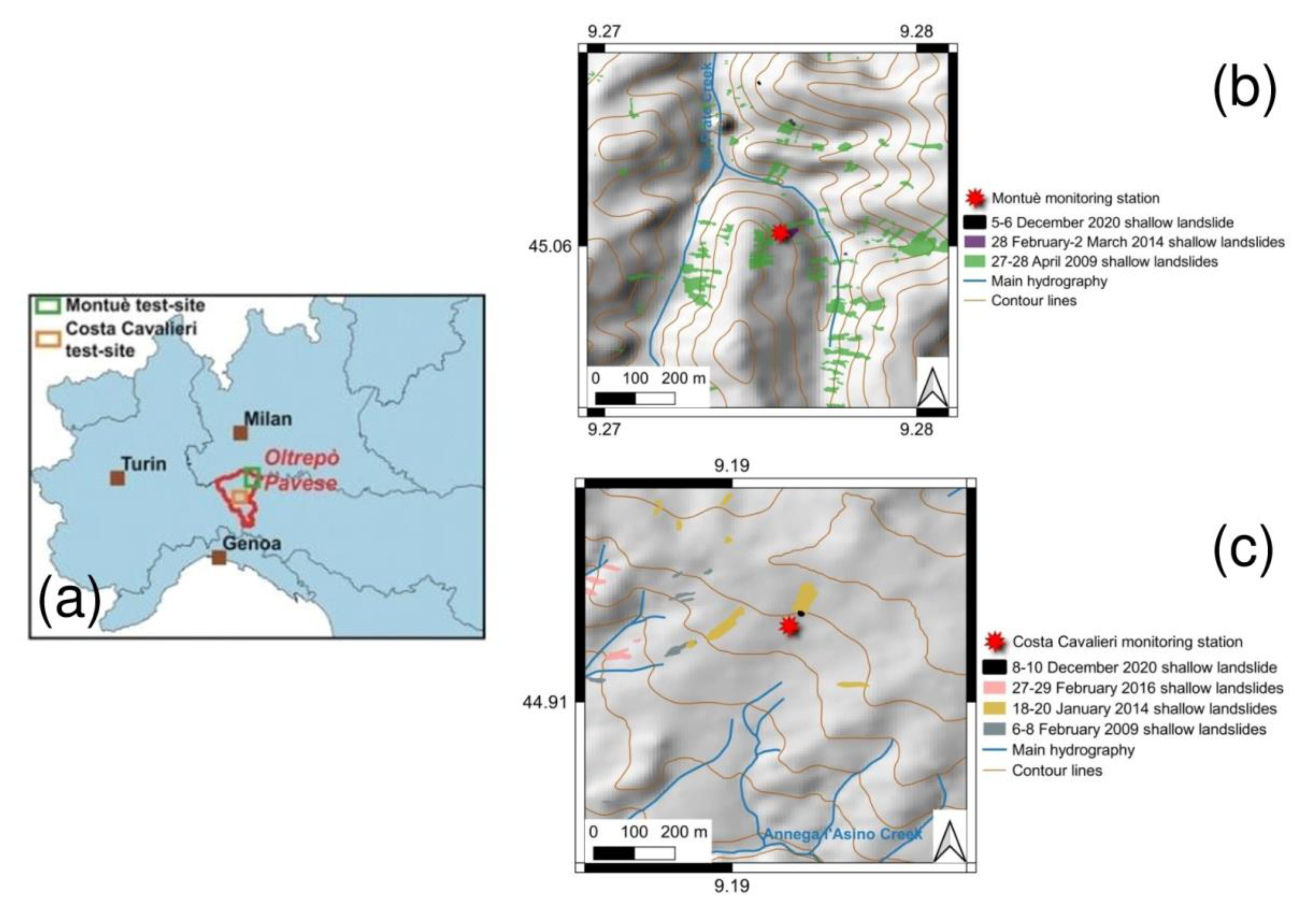
SWP measurements were acquired in two test-sites of Oltrepò Pavese area (northern Italian Apeninnes,
Figure 1).
The former is located near the village of Montuè (
Figure 1b) in north-eastern OltrepòPavese. It has very steep slopes (26–35°), medium-low elevation (170–210 m a.s.l) and land use characterized by shrubs and woodlands of black robust trees. The bedrock is made of gravel, sand and poorly cemented conglomerates overlying marls.
The latter is located near the village of Costa Cavalieri, (
Figure 1c) in central Oltrepò Pavese. It has medium-low slope steepness (7–18°), medium elevation (460–500 m a.s.l.) and land use characterized by sowed fields. The bedrock is composed of a clayey mélange, with scattered calcareous and marly blocks that can reach metric dimensions.
In both the sites, the climatic regime is temperate/mesothermal. The mean yearly temperature is of 11–12 °C and the mean yearly rainfall depth is around 700–720 mm.
The areas are very prone to shallow landsliding, as testified by some events occurred in 2009, 2014 and 2016 (
Figure 1) [
31,
32].
The following laboratory tests were carried out on samples of the different soil levels of the test-sites according to the American Society for Testing and Materials (ASTM): (i) grain size analyses and Atterberg limits on disturbed samples; (ii) Drive-Cylinder Method for the measure of volumetric features of undisturbed samples; (iii) measure of carbonate content of disturbed samples through a calcimeter; (iv) oedometric tests on undisturbed soil samples; (v) determination of the shear strength parameters in drained conditions after consolidation (effective stress). In particular, as for Montuè soil layers, peak shear strength parameters were determined on undisturbed soil samples through CID triaxial tests, under isotropic confining stresses comparable to those in situ at shallow depths. No dilatant effect was observed. As for Costa Cavalieri soil levels, residual shear strength parameters on undisturbed soil samples were obtained through direct shear tests, since this soil had been affected by past shallow landslides [
33].
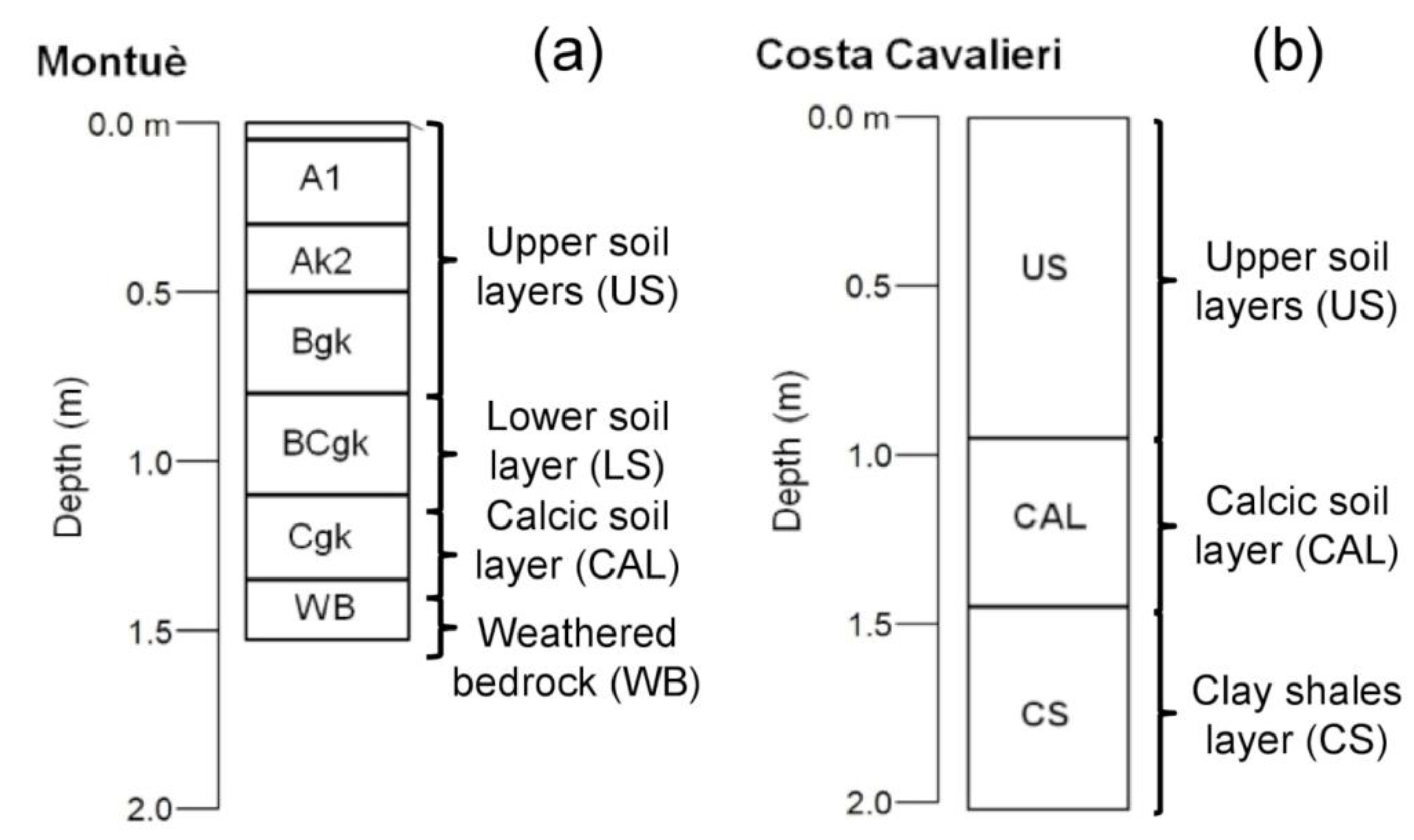
At Montuè, superficial soils derived by bedrock weathering are prevalently clayey-sandy silts and clayey-silty sands, with a peculiar succession of layers (
Figure 2a,
Table 1). A detailed description of this profile is present in [
31,
32]. From the ground surface down to 0.7 m, the upper soil layer (US) is characterized by a clayey-sandy silt texture with low plasticity, high content in carbonates, as soft concretions, and unit weight in the order of 16.7–17.0 kN/m
3. Superficial soil layers of Montuè were affected by tillage operations for grapevines cultivation in the past century, determining remolding and low density of the materials [
31]. Below them, the lower soil layer (LS) between 0.7 and 1.1 m from the ground is characterized by similar texture, plasticity and carbonate content, but bigger unit weight (18.6 kN/m
3). At a depth between 1.1 and 1.3 m, a calcic horizon (CAL) maintains the same textural, plasticity and density features of the LS one, but it shows a significant increase in carbonate content, up to 35.3%. Soil levels typically have porosity of 43–49%. The weathered bedrock (WB) is 1.3 m from the ground surface.
The identified soil layers can be distinguished also by their mechanical and hydrological features. US and LS are characterized by similar peak friction angle, equal to 31 and 33°, respectively, and by a nil effective cohesion. Instead, CAL horizon has a lower value of the friction angle (26°), but an effective cohesion of 29 kPa. All the soil levels are slightly over consolidated due to the past tillage operations and the continuous cycles of drying and wetting, besides the presence of a low amount of clayey minerals [
31].Saturated hydraulic conductivity, measured in field through an amoozometer, decreases along depth. US has the highest value along the soil profile, in the order of 10
−5 m/s, while LS and CAL are characterized by a saturated hydraulic conductivity lower than US of 1 and 2 orders, respectively (10
−6 m/s for LS, 10
−7 m/s for CAL).
At the Costa Cavalieri test-site, silty clay soils derived by bedrock weathering are present. Three main soil layers can be identified (
Figure 2b,
Table 2). From the ground surface down to about 0.9 m, the soil (upper soil layer US) is characterized by a silty clay texture with high plasticity, high content in carbonates, as soft concretions, and unit weight in the order of 18.7–19.0 kN/m
3. Below this level, between 0.9 and 1.4 m, there is a calcic soil layer (CAL). It is characterized by similar texture and plasticity with respect to the upper one, but it presents a higher unit weight (20.3 kN/m
3) and higher carbonate content (26.7%) than US level. In this layer, carbonate concretions are significantly compact and their size ranges between centimeter to decimeter. Between 1.4 and 2.0 m, a further layer maintains the same textural and plasticity of CAL, but is characterized by lower unit weight (19.3 kN/m
3) and by a nil content in carbonates. This layer can be identified as a clay shales layer (CS), due to its soft and very plastic consistency when it is wet. Soil levels have typically porosity of 37–45%. Weathered bedrock levels can be identified only at higher depths, generally at about 3.5–4.0 m from ground level.
As for Montuè typical soil profile, the soil layers at Costa Cavalieri site can be distinguished also by their mechanical and hydraulic features. US and CS are characterized by similar values of residual friction angle, equal to 10 and 12°, respectively, instead CAL layer has a higher residual friction angle, equal to 18°. All soil layers are characterized by a nil effective cohesion. Moreover, the soil levels are only slightly over consolidated due to the continuous cycles of drying and wetting and for the presence of clayey minerals [
33]. Saturated hydraulic conductivity, measured in field through an amoozometer, decreases along depth. US has the highest value along the soil profile, in the order of 10
−5 m/s, while CAL and CS are characterized by a saturated hydraulic conductivity lower than US of 2 and 3 orders, respectively (10
−7 m/s for CAL, 10
−8 m/s for CS).
2.2. Field Monitoring Equipments
In both test-sites, a hydrological monitoring station collecting data with a time resolution of 10 min was installed.
At Montuè test-site, the station was installed in March 2012. It integrates meteorological and hydrological sensors. The meteorological sensors measure rainfall, air temperature, air humidity, atmospheric pressure, wind speed and direction, net solar radiation. Some hydrological sensors for the measure of SWP were installed at 0.2, 0.6, 1.2 m from the ground level. A coupled system of tensiometers (Model Jet-Fill 2725, Soil moisture Equipment Corporation, Santa Barbara, CA, USA) and heat dissipation sensors (Model HD229, Campbell Scientific, Logan, UT, USA) allow to cover the full regime of SWP from close to saturation (through tensiometers) to unsaturated (through heat dissipation sensors) soil conditions at each monitored depth. The accuracy of both these devices is of 0.1–0.2 m. A more detailed description of the structure of this station is in Bordoni et al. [
31].
The Costa Cavalieri station was installed in November 2015. It allows to measure SWP temporal trends at 0.4, 0.6 and 0.9 m from the ground level. A coupled system of tensiometers (Model T4e, UMS GmbH, Munich, Germany) and dielectric sensors (Model MPS-6, Decagon Devices, Pullman, WA, USA) allowing to cover the full regime of SWP from close to saturation (through tensiometers) to unsaturated (through dielectric sensors) soil conditions at 0.6 and 0.9 m from ground. A dielectric sensor is located at 0.4 m from ground, allowing to measure SWP values lower than −1 m. The accuracy of Costa Cavalieritensio meters is 0.1 m, while the one of the dielectric sensors is 0.3 m. Meteorological data for Costa Cavalieri station (rainfall amount, air temperature, air humidity, wind speed and direction) were acquired by the meteorological station of ARPA Lombardia meteorological network, which is located 2 km from the monitoring station. A more detailed description of the structure of this station is in Bordoni et al. [
33].
At 0.2 m in the Montuè site, SWP in the range between 0 and −1 m has not been acquired since November 2012 due to the breakage of the tensiometer.
Due to the height of the water column present in these device, tensiometers data need to be corrected of 0.1 m for each 10cm of depth in the soil. In this way, positive values of SWP could also be acquired [
34].
2.3. Machine Learning Methods
Machine Learning (ML) groups are a set of statistical methods of artificial intelligence concerned with the design and development of algorithms thus allowing to evolve behaviors and to develop models of a particular phenomenon based on empirical data [
35]. ML algorithms aim to develop regression or classification models [
35,
36]. For regression purposes, ML models build the relationships able to estimate a response variable based on one or more predictors, even if these relationships cannot be easily written as functions [
35].
As other data driven methods, ML techniques are differentiated on the basis of the type of algorithms which control the search to find and build the knowledge structures, representing the relations between the output response and the input predictor variables. In particular, Supervised Machine Learning aims to find the best-fit relationships between predictors and response variables, which minimize the squared errors between measured and modeled values of response [
36].
Different ML methods have been applied to solve different regression problems in hydrology [
22,
37]. Since no robust methodologies have been already developed to estimate temporal trends of SWP, several ML techniques have been tested in this work to find the best models to solve effectively the assessment of SWP in time. The seven selected methods correspond to the ones most adopted for solving regression problems in soil hydrology [
37,
38].
Artificial Neural Networks are based on a collection of connected units or nodes, which can allow to estimate complex relationships between independent predictors to generate the correct measures of a response variable, whose values are influenced by the input parameters of the model.
Support Vector Machines with radial kernels are able to estimate the values of a response variable capturing the effects of each predictor by separating the input dataset with a hyperplane in a high-dimensional space.
Random Forests are based on an ensemble of multiple decision trees, generated based on the values of an independent set of random predictors adopted to find the best prediction of the output response variable.
Relevance Vector Machines have a similar approach to Support Vector Machines, but they employ an additive noise term to minimize the random errors between the real measured and estimated values of the response variable of a model.
Bayesian Linear Regression is based on a multiple linear regression model to estimate a response variable from a set of probability distributions of the input predictors of the model, in order to reconstruct more robust relationships to estimate all the possible values of the output.
Gradient Boosting Regression Trees are tree ensemble methods that build a decision tree learner to estimate a response variable by fitting the gradients of the residuals of the previously constructed tree learners starting from the input predictors of the model.
Deep Learning Regression Networks are methods that emulate the decision making of the human brain, building up linked relationships between the predictors to estimate different possible values of the output response variable.
We refer to Matloff [
35] and Harrington [
36] for more explanations and for the main mathematical principles of the different ML techniques tested in this work.
2.4. Datasets
SWP temporal trends at different depths collected at both test-sites with daily resolution were used to build and to validate the machine learning models. For the Montuè test-site, the time span between 27 November 2012 and 25 May 2020 (about 90 months) was considered, while the monitoring period at Costa Cavalieri test-site was between 3 March 2016 and 25 May 2020 (about 50 months). SWP trends were reconstructed at two different depths in both test-sites, in order to develop models able to estimate the hydrological dynamics in different soil horizons. Based on the availability of continuous acquired time series, SWP trend monitored at 0.6 and 1.2 m and at 0.6 and 0.9 m from ground were considered in Montuè and Costa Cavalieri, respectively.
Three types of predictors were considered in the data-driven models. The first set corresponds to the daily values of the main meteorological parameters, which can influence the fluxes interesting soils at daily time span (e.g., evaporation, rainwater infiltration) [
15,
39]: rainfall amount, air temperature, air humidity, solar radiation, wind speed. These parameters were acquired in correspondence with the monitored test-site at Montuè. Instead, for the Costa Cavalieri test-site, the measures of these parameters were acquired at two meteorological stations of Arpa Lombardia monitoring network (Fortunago and Varzi-Nivione stations), located close to this monitored test-site (lower than 15 km) in a similar range of altitude (400–500 m a.s.l.).
The second set of predictors was composed by meteorological parameters that can be considered as proxies of the antecedent meteorological conditions, which can provoke different responses in soil-water dynamics even if the daily values of meteorological parameters are quite similar [
40]. By considering cumulated rainfall amount of 3, 7, 14, 30, and 60 previous days and the mean air temperature of 3, 7, 14, 30, and 60 previous days it was possible to take into account the effects of antecedent conditions of different time spans (weekly, monthly, and seasonal) in soils characterized by a silty or clayey texture [
41]. These parameters were calculated for each day of the modeled trends, starting from the day before a selected date.
The third set of predictors was represented by antecedent SWP values. Observed soil hydrological conditions in a day often do not correspond only to antecedent rainfall indexes [
41], due to the complex subsurface hydrological processes and drainage systems. In fact, especially during concentrated thunderstorms occurred when soils are particularly dry, non-equilibrium lags are often observed [
7,
31,
42]. This may cause biases that limit the reliability of models aiming to explain soil-water content or soil-water potential dynamics in time [
43]. Moreover, the predictability of the water status in a soil also depends on the medium-short soil moisture memory characteristics, especially in soils with fine texture and medium-low permeability [
40]. Due to these reasons, mean values of SWP of the three and seven previous days were considered to explore the possible effects of SWP memory on the predictability of actual values of SWP. These two predictors were calculated as the average of the modeled values of SWP at three and seven days before a certain date, respectively.
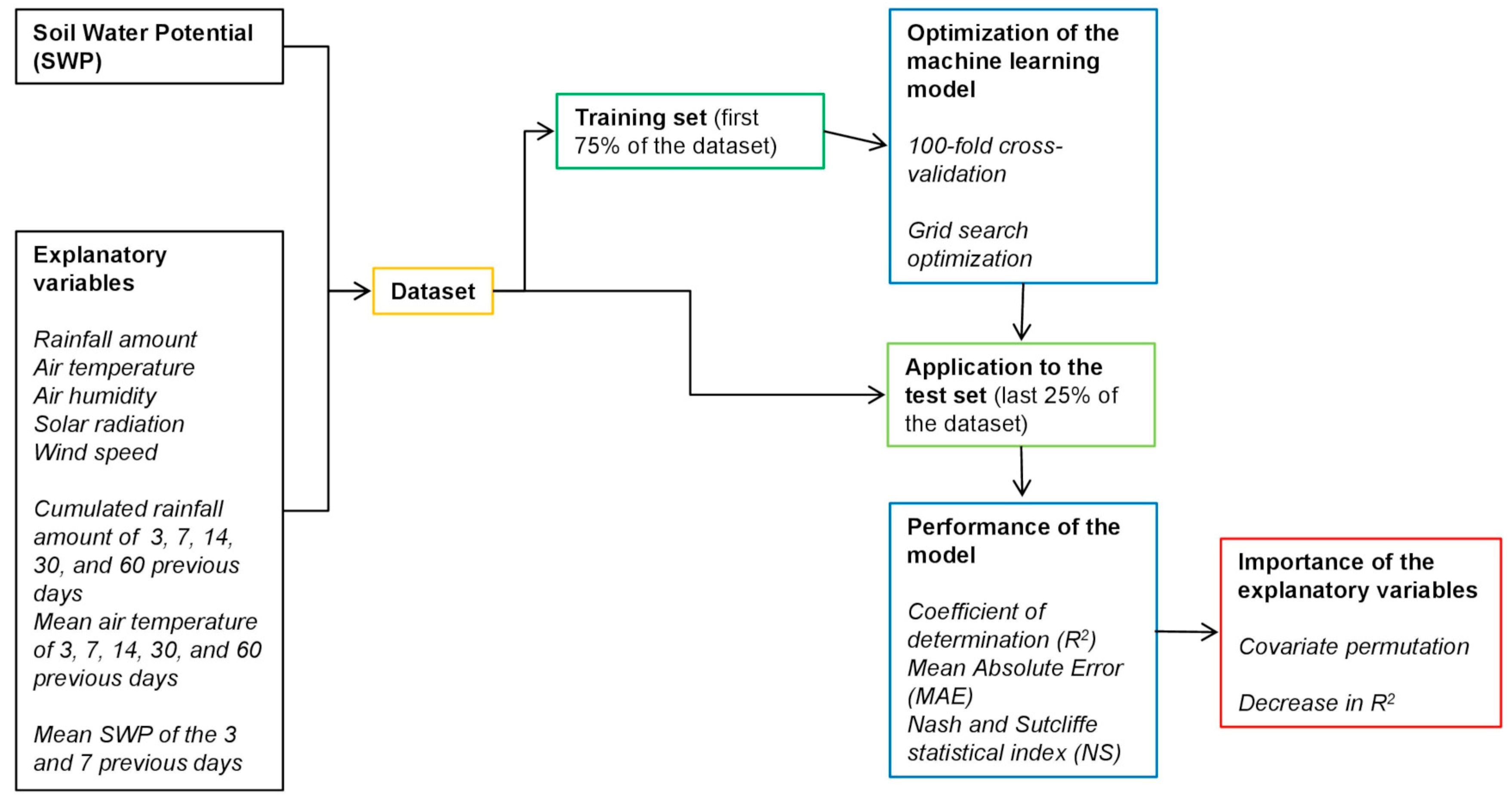
2.5. Setup of the Data-Driven Approach
Figure 3 summarizes the implementation steps of the machine learning approach adopted to estimate temporal trends of SWP.
The developed data-driven model aimed to reconstruct daily temporal trends of SWP at a particular soil depth of a test-site. Daily SWP was estimated finding the best relationships between the response variable and the parameters considered as its predictors.
All the daily predictors were used to train models of SWP prediction for each of the considered statistical techniques. The dataset was divided into a training and test subset, where the training was bigger than the test one. In particular, the first 75% of the temporal series constituting the dataset was used to train a model, while the remaining 25% of the temporal series represented the subset for test and validation. These percentages were chosen to obtain a long set of acquisition required to build a model able to represent all the possible hydrological conditions the soil layers could experience [
35,
37].
A 100-fold cross-validation and grid search optimization were used to optimize the parameters required by each statistical technique to fit the best regression model between the explanatory and the response variables of the training dataset [
35]. The obtained model was then applied to the test set. The model predictive capability of real daily SWP values was estimated through three statistical indexes, namely the coefficient of determination (R
2), the mean absolute error (MAE) and the Nash and Sutcliffe statistical index (NS). The best machine learning method with the best effectiveness in reconstructing the measured temporal trends of SWP was the one characterized by the lowest values of MAE and RMSE and by the highest positive value of NS.
Considering that not all the predictor variables at analyzed soil depth can improve the SWP prediction, a sensitivity analysis of the importance of each variable in each selected machine learning model was carried out by means of the covariate permutation [
28,
44]. This was done by permuting each predictor variable at a time, while leaving the others unchanged, and tracing the decrease in a performance metric, that corresponded to R
2 as typically adopted for this aim [
44]. This analysis was performed on both the models for training and test subsets, in order to give insight on the ranking of predictors’ importance for each simulation, which could ultimately provide increased interpretability on the achieved results. In the case of an alleged low importance for a predictor when being permuted individually [
45], also permutation of groups of predictors that were related physically was also performed.
After these analyses, it might be possible that some predictors variables could influence negatively the prediction or did not cause a significant improvement on the predictive capability. Thus, the final model for each analyzed soil layer was the one with the optimal set of predictors which could effectively simulate the measured SWP trends avoiding problems of overfitting or bias [
35,
44].
2.6. Implementation of Modeled SWP in the Prediction of Rainfall-Induced Shallow Landslides
The validation of the developed models for SWP estimation was carried out by implementing the modeled trends in further methodologies, used to predict the temporal occurrence of rainfall-induced shallow landslides at both the test-sites.
The identified best models for SWP prediction at different depths at both test-sites were used to simulate daily temporal trends of SWP for other timespans, i.e., the period between 1 October 2020 and 6 January 2021. For this analysis, a set of daily values of the model predictors was reconstructed and implemented in each selected model to obtain the daily values of SWP as output. The values of the predictors were obtained from the same monitored points where training and test sets of the models were collected (Montuè monitoring station for Montuè test-site; Fortunago and Varzi-Nivione meteorological stations of Arpa Lombardia for Costa Cavalieri test-site).
During the simulated timespan, an incipient shallow landslide with sliding surface at 0.6 m from ground level occurred on 5 December 2020, 500 m far from the Montuè test-site towards the northern direction, in a very steep slope (slope angle of 32°) with soils having profiles similar to those observed at the monitored slope. Moreover, a shallow landslide with sliding surface at 0.9 m from ground level was triggered on 9–10 December 2020 in Costa Cavalieri test-site, on the same hill 47 m above the monitoring station, where the slope angle is 8°.
First, the modeled SWP trends at the two soil layers where shallow landslides sliding surfaces developed in December 2020 were reconstructed by means of the identified best models. The obtained SWP trends were inserted in a slope stability model based on infinite slope assumption, consistent with the limited depth of the sliding surfaces compared with the length of the considered slopes (183–196 m), and for generalized effective stress in soil [
46]:
where
Fs is the slope safety factor,
φ is the soil friction angle,
β is the slope angle,
c′ is the soil effective cohesion,
ψ is the SWP,
γw is the water unit weight (set equal to 10 kN/m
3),
γ is the soil unit weight,
z is the depth where the sliding surface developed,
β is the slope angle.
Table 3 summarizes the values of the input parameters required by this model for reconstructing FS trends along the analyzed time span.
In the model for Fs calculation, the first term on the right-hand side of Equation (1) allowed to consider the internal frictional resistance of the soil. The second term of Equation (1) took into account separately the effects of soil effective cohesion and of SWP. The more negative is the value of SWP (unsaturated conditions), the higher is the overall effect of this parameter in increasing shear strength and decreasing the proneness to the triggering of shallow failures [
7]. In contrast, for nil or positive values of SWP (saturated conditions), the higher is the value of SWP, the bigger is the reduction of effective stresses(and then soil shear strength) with a consequent increase in the proneness of shallow landslide triggering [
7].
Furthermore, the same modeled trends of SWP were used to select the appropriate physically-based rainfall threshold from the three reconstructed for the area where both the test-sites are located.
These thresholds were reconstructed applying TRIGRS model [
46] considering the soil profiles and properties of the test-sites (
Table 1 and
Table 2). The modeling was carried out considering different constant rainfall events with duration varying in the range of 1–200 h and cumulative values varying in the range 1–1000 mm. Each of these rainfall events were simulated considering three selected SWP conditions in the soil at the beginning of the event, namely lower than −1, −1 and 0 m. Results of the hydrological modelling were used to perform slope stability analyses at typical failures depth(up to 1.0 m from ground level). These calculations allowed to identify critical conditions leading to shallow landslide triggering (
Fs ≤ 1), discriminating rainfall events with no slope failures (
Fs > 1). As a result, different thresholds for the selected initial SWP conditions were reconstructed. Fitting equations of these thresholds are listed in
Table 4. Further explanations on the method of thresholds reconstruction are in Bordoni et al. [
32].
SWP at the beginning of a certain rainfall event corresponded to the simulated value of the day before the rain started to fall in that event. According to this value of SWP, one of the three reconstructed thresholds was selected: (i) threshold for SWP lower than −1 m, if simulated SWP was lower than −1 m; (ii) threshold for SWP of −1 m, if simulated SWP approximated −1 m; (iii) threshold for SWP of 0 m, if simulated SWP approximated or were over 0 m. Cumulated rainfall in mm (E) and duration (D) of each event were calculated. The point corresponding to each pair D-E was compared with the selected rainfall threshold, allowing to distinguish events below the threshold, that did not provoke landslide triggering, from events above the thresholds, which caused the triggering of slope failures.
3. Results
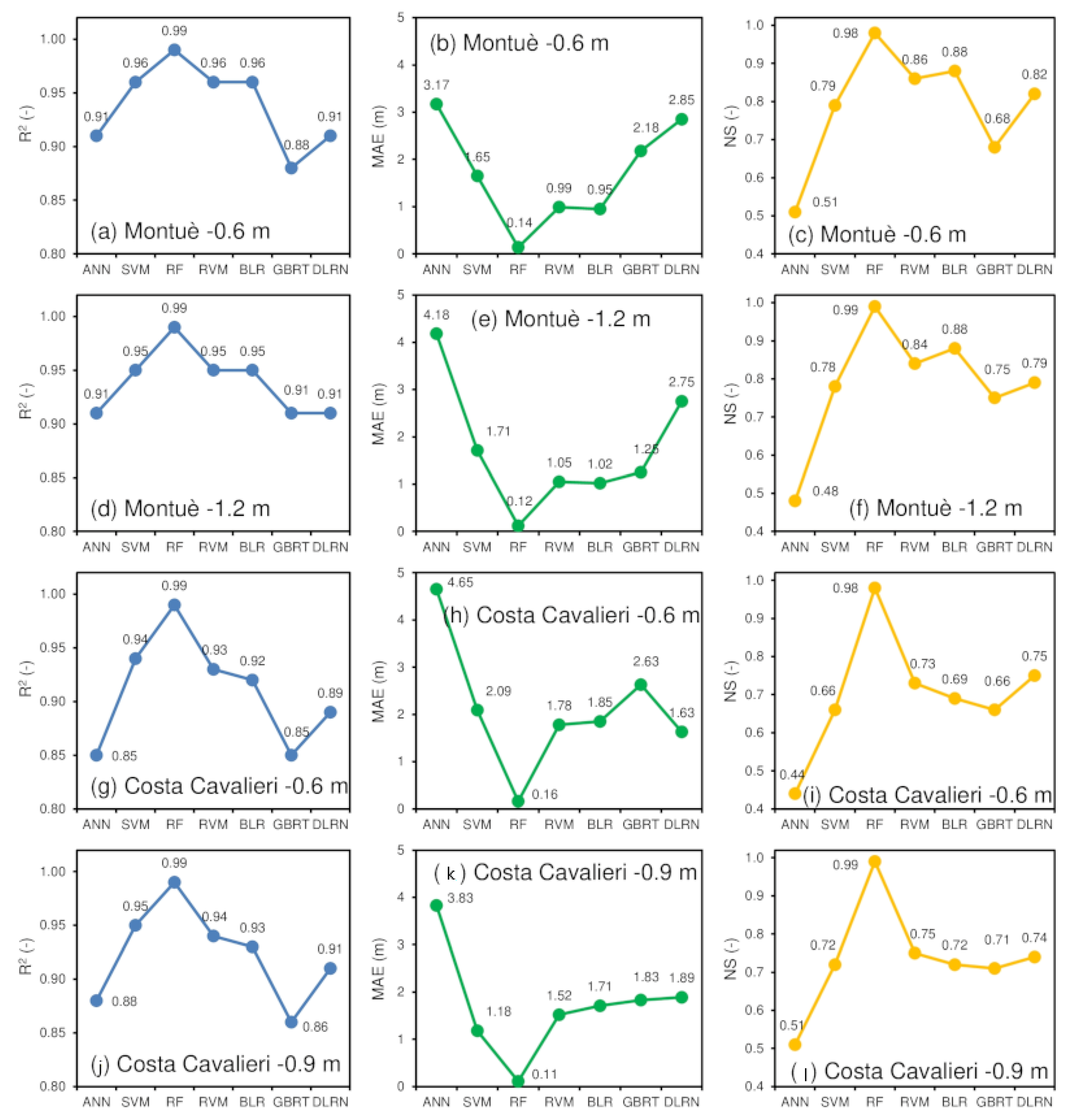
3.1. Machine Learning Models
Performance indexes of the SWP models obtained by different statistical methods based on the training dataset were similar, in the range 0.90–0.99, 0.01–1.03 m and 0.90–0.99 for R
2, MAE and NS, respectively. The highest differences on the performance of the different statistical techniques were more evident considering the models for the test sets (
Figure 4), allowing to determine the best machine learning method able to predict SWP trends in different soil layers.
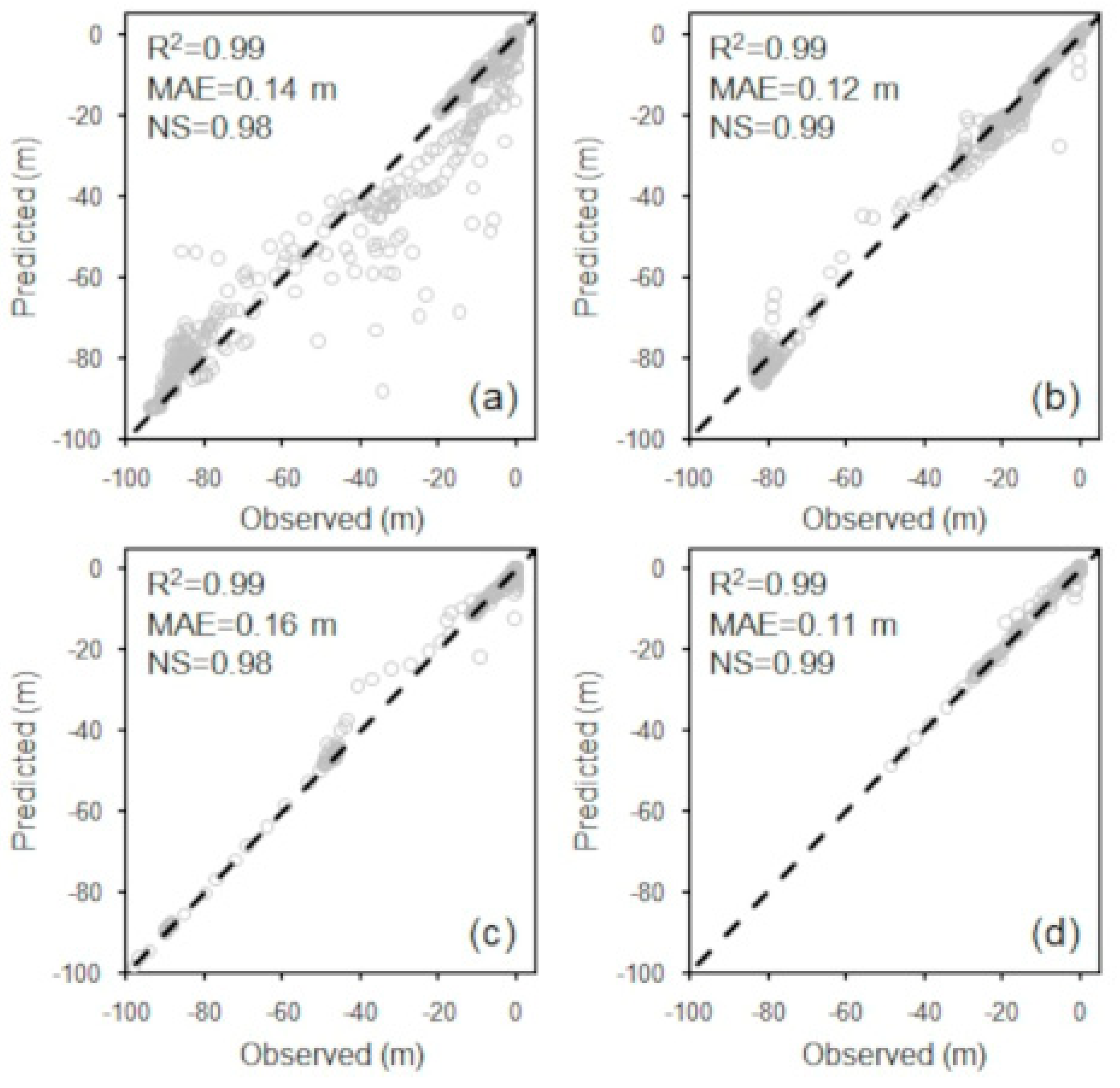
The performance indexes related to test sets presented significant differences between measured and modeled SWP trends. Even if all the techniques were characterized by high values of R2 (higher than 0.85) for all the tested soil depths, the models based on Random Forests (RF) performed significantly better than the other techniques, since R2 of these models were equal to 0.99 for all the modeled trends. The goodness on the predictive capability of RF models was confirmed by the lowest values of MAE (between 0.11 and 0.16 m) among the different tested machine learning methods for the different tested soils. Furthermore, RF models allowed to estimate the temporal hydrological trends of all the layers in the best way with respect to the other tested techniques, since NS values ranged between 0.98 and 0.99. The close range of the different performance metrics demonstrated the similar and outstanding capability of RF models to estimate the temporal trends of SWP in soil levels characterized by different features and located at different depths.
The effectiveness of RF models in simulating SWP trends was highlighted also through the scatterplots, with the observed values against the simulated ones (
Figure 5). The observed SWP-simulated SWP pairs were located very close to the 45° line (dotted line), confirming the capability of these models to estimate correctly the daily trends of soil water potential in the different tested soil layers.
Residual values were also calculated to determine the model certainty in the analyzed test sets (
Figure 6). The widest residual fluctuation of RF models related to the test sets was in the range (−5.1, 7.4) m. Moreover, the mean and median values of the residuals were in the range (0.0, 0.8) m and (0.0, 0.9) m, respectively. The distributions of residuals, together with the low values of the MAE, confirmed how the RF modeled values were very realistic for all the tested soil layers. The distributions of residuals were smaller for Costa Cavalieri soils than those for Montuè, as shown by the closest amplitude between the minimum and the maximum residuals ((−1.3, 1.4) m at 0.6 m, (−0.3, 0.3 m) at 0.9 m) and by mean and median values around 0.0 m.
3.2. Sensitivity to Model Predictors
The sensitivity of the best machine learning models used to estimate SWP trends in the different tested soils, which corresponded to the RF ones, was assessed based on the decrease in R
2 as a consequence of permuting a covariate or a set of similar covariates (
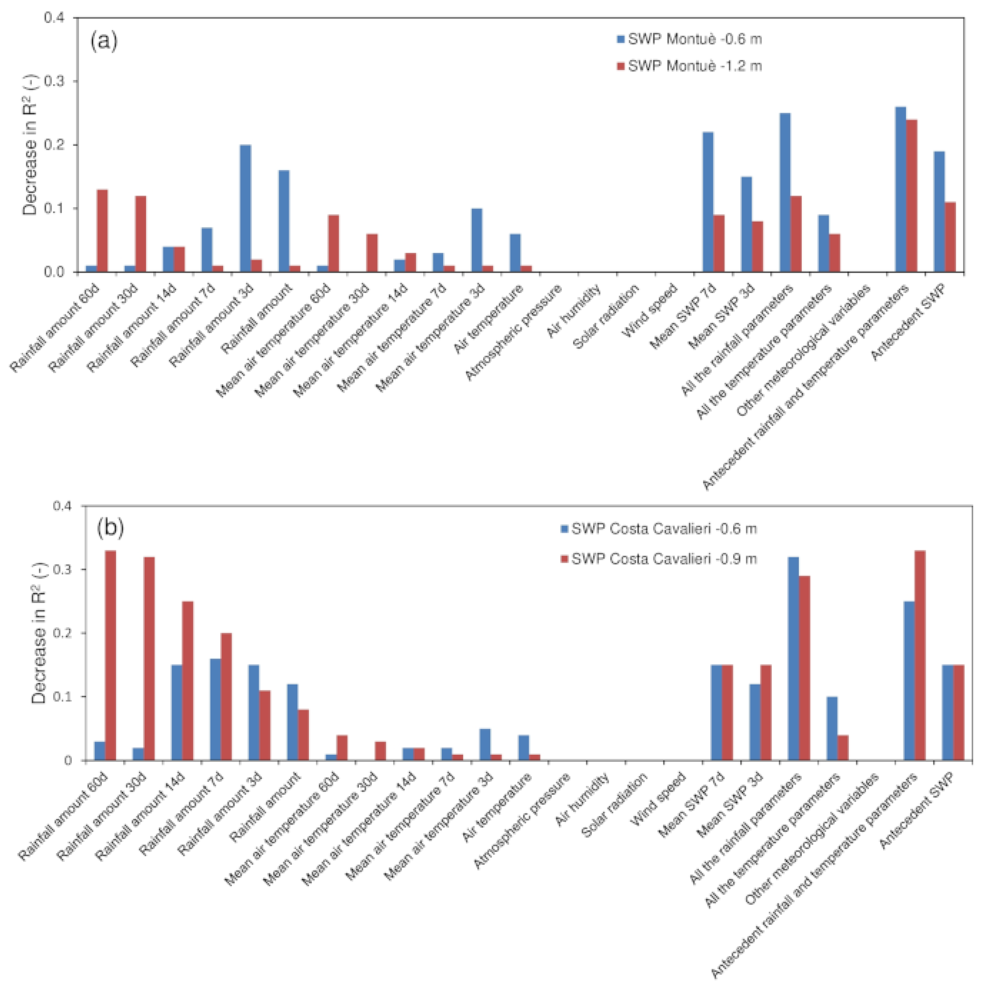
Figure 7). These analyses allowed to determine the relative ranking of the most sensitive predictors for each simulated SWP trend.
For the layers at 0.6 m from ground of both test-sites, cumulated rainfall amounts of short intervals were the most important meteorological predictors to model SWP. A decrease in R2 between 0.12 and 0.20 was detected when rainfall amounts of 3, 7 and 14 days were permuted. The other meteorological variables caused a more limited reduction in the predictive capability of the model, as testified by decrease in R2 lower than 0.06. Atmospheric pressure, air humidity, solar radiation and wind speed had nil effects on the performance of these models, since their permutation did not cause any reduction in R2. To model SWP trends at 0.6 m in both test-sites, antecedent average SWP values of the previous 3 and 7 days had a significant impact, as confirmed by a reduction in R2 of 0.12–0.15 and of 0.15–0.22 considering mean SWP of the previous 3 days and mean SWP of the previous 7 days, respectively.
For the deepest layers of both the test-sites, cumulated rainfall amounts in longer time spans were the most influencing predictors to model SWP.
At 1.2 m in Montuè test-site, the dominant meteorological predictors were the cumulated rainfall amounts of the previous 30 and 60 days, whose permutation caused a reduction in R2 of 0.09 and 0.15, respectively. At 0.9 m in Costa Cavalieri test-site, the dominant meteorological predictors were the cumulated rainfall amounts of the previous 7, 14, 30 and 60 days, whose permutation caused a reduction in R2 between 0.20 and 0.33. As for the shallowest soil layers, the other meteorological predictors caused a more limited reduction in the predictive capability of these models, as testified by decrease in R2 lower than 0.06.
Furthermore, atmospheric pressure, air humidity, solar radiation and wind speed had nil effects on the performance of these models, since their permutation did not provoke any reduction in R2. As for the prediction models of the soil layers at 0.6 m from ground, the impact of antecedent SWP (average SWP of the previous 3 and 7 days) was evident for the correct estimation of the actual daily water potential. The decrease in R2 was of 0.17–0.18 at 1.2 m in Montuè test-site and of 0.15 at 0.9 m in Costa Cavalieri slope.
The importance of physically related explanatory variables was also quantified. The impact of rainfall attributes in modeling SWP at different depths of different contexts was confirmed by the high values of reduction in R2 for all the tested soils (0.12, 0.25) for Montuè, (0.29, 0.32) for Costa Cavalieri). Furthermore, SWP in all the tested soils was very sensitive to antecedent rainfall and temperature attributes, especially for the levels located more in depth in the soil profile. In fact, the reduction of R2 due to the permutation of antecedent rainfall and temperature parameters increased from 0.26 to 0.28 passing from 0.6 to 1.2 m in Montuè, from 0.25 to 0.33 passing from 0.6 to 0.9 m in Costa Cavalieri. The drop in performance of the models was nil when the other meteorological variables (atmospheric pressure, air humidity, solar radiation and wind speed) were permuted. The collective permutation of antecedent SWP confirmed the significant impacts of these attributes in modeling actual daily SWP in all the analyzed contexts, since the decrease in R2 was of (0.18, 0.19) in Montuè and of 0.15 in Costa Cavalieri.
3.3. SWP Trends
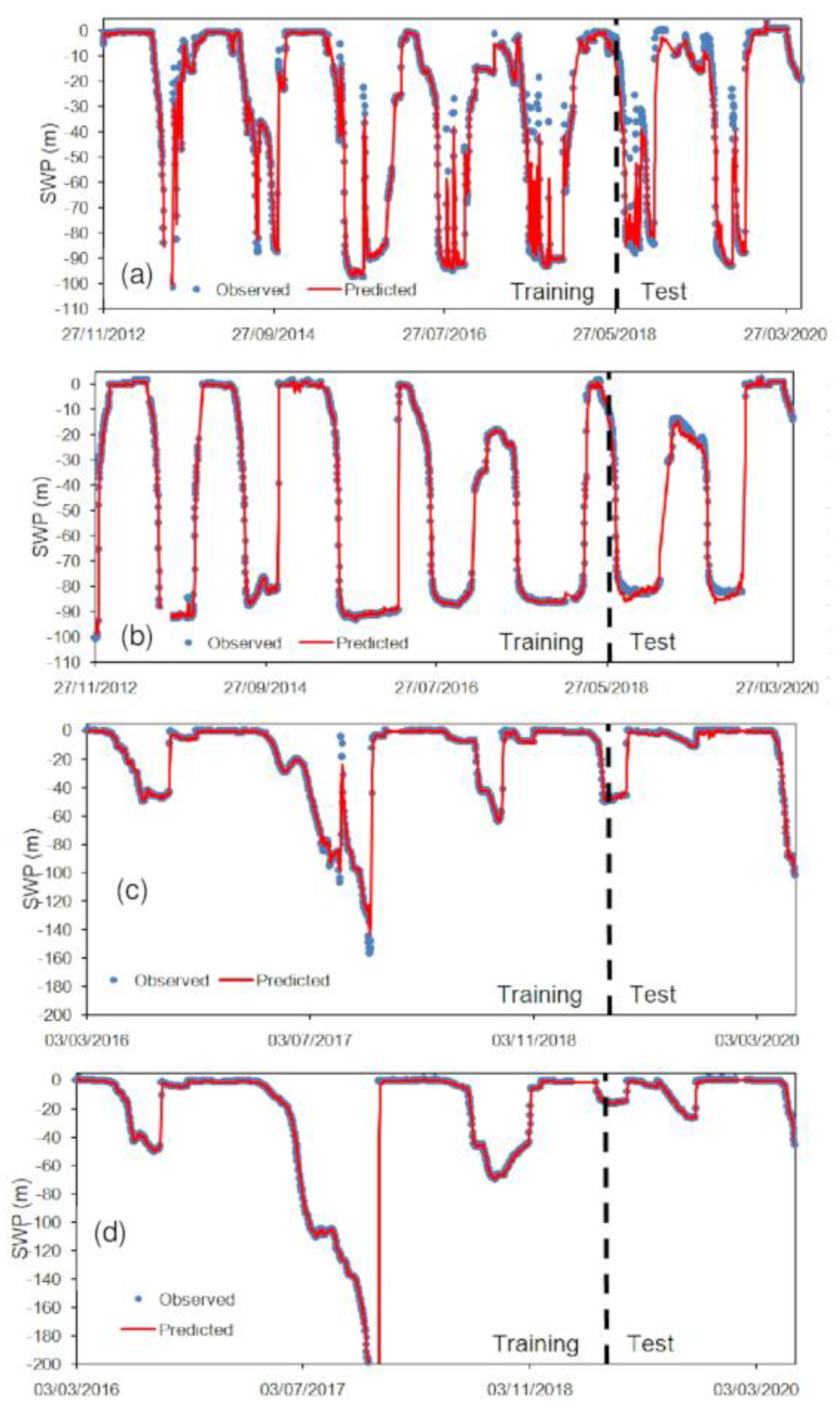
The chosen machine learning models (RF models) allowed to reconstruct correctly the temporal trends of SWP at different depths of both test-sites, identifying the variation of hydrological behaviors throughout the different seasons and in relation to dry and wet periods (
Figure 8).
The modeled SWP trends obtained through RF method for all the tested soils remained unchanged considering the entire set of predictors or neglecting atmospheric pressure, air humidity, solar radiation and wind speed, since the influence of these meteorological variables was irrelevant in the estimation of SWP dynamics.
SWP dynamics showed dry phases, when soils experienced values of SWP down to −100 m, alternated with wet periods, when SWP was close to 0 m or could reach positive values.
In both sites, during typically rainy periods between November and March, soil conditions near saturation (SWP > −1 m) to complete saturation were observed and modeled correctly by the RF approach. The higher the amount of fallen rain was during these months, the longer the period was with conditions close to saturation in the cover: 20–35 days with an average cumulative rainfall of 241 mm, 138 days with a mean value of 337 mm. In these conditions, the soil level at 0.6 m of Montuè site approached complete saturation, while the layer at the same depth in Costa Cavalieri site could get also positive values up to 0.5 m.
Instead, the deepest monitored soil layers of both test-sites, located at 1.2 and 0.9 m in Montuè and Costa Cavalieri, respectively, could reach fully saturated conditions and a transient water table could form. At Montuè test-site, SWP could reach values up to 1.2 mat 1.2 m from ground. At Costa Cavalieri test-site, SWP could reach 0.9 m at 0.9 m of depth.
In summer months, the decrease of the SWP was faster in shallowest soil horizons than in the deeper ones. In July and August, the driest condition was observed at both test-sites. SWP could reach values around −100 m in the entire soil profile at Montuè and values in the range (−200, −160) m at Costa Cavalieri.
Finally, autumn months were a transition period, when SWP could increase significantly in consequence of the increase in rainfall events and the decrease of evapotranspiration processes. Re-wetting of the soil layers down to 0.6m from ground attained SWP values close to −1 m during rainfall events in October and November at both test-sites. Instead, the saturation of the deepest layers occurred typically since the end of November, when rainwater infiltration became more abundant and SWP could reach values of −2/−1 m at 1.2 m from ground level at Montuè test-site and at a depth of 0.9 m at Costa Cavalieri test-site.
Considering a monitoring period common to both test-sites, soil-water potential values in the different soil layers kept higher than −1 m only during 20–35 days between December and May 2016, 2017 and 2019, characterized by a limited amount of rain fallen in the cold months (averagely 241 mm and 251 mm of cumulated rainfall between December and May at Montuè and Costa Cavalieri, respectively). Instead, between December and May 2018, soil-water potential values in the different soil layers of the two test-sites kept higher than −10 m for 138 days, as a consequence of a rainier period (337 mm and 406 mm of cumulated rainfall between December and May at Montuè and Costa Cavalieri, respectively) than in other years.
3.4. Prediction of Rainfall-Induced Shallow Landslides Based on Implementation of Modeled SWP Trends
The selected machine learning models (RF models) were applied to predict the temporal trends of SWP at the same observed depths where shallow landslides occurred during the period 1 October 2020–6 January 2021,i.e., 0.6 m at Montuè and 0.9 m at Costa Cavalieri test-site. In particular, the initial value of SWP was equal to −40 m at 0.6 m at Montuè and equal to −10
2 m at 0.9 m at Costa Cavalieri. These values had been measured by each monitoring station at the beginning of the modeled time span. SWP modeled trends were, then, implemented in the calculation of the factor of safety (Fs) for each slope at Montuè and Costa Cavalieri test-site, respectively. This allowed us to reconstruct Fs trends and to verify the reliability of the modeled SWP in predicting the triggering of shallow landslides in the expected date (
Figure 9 and
Figure 10).
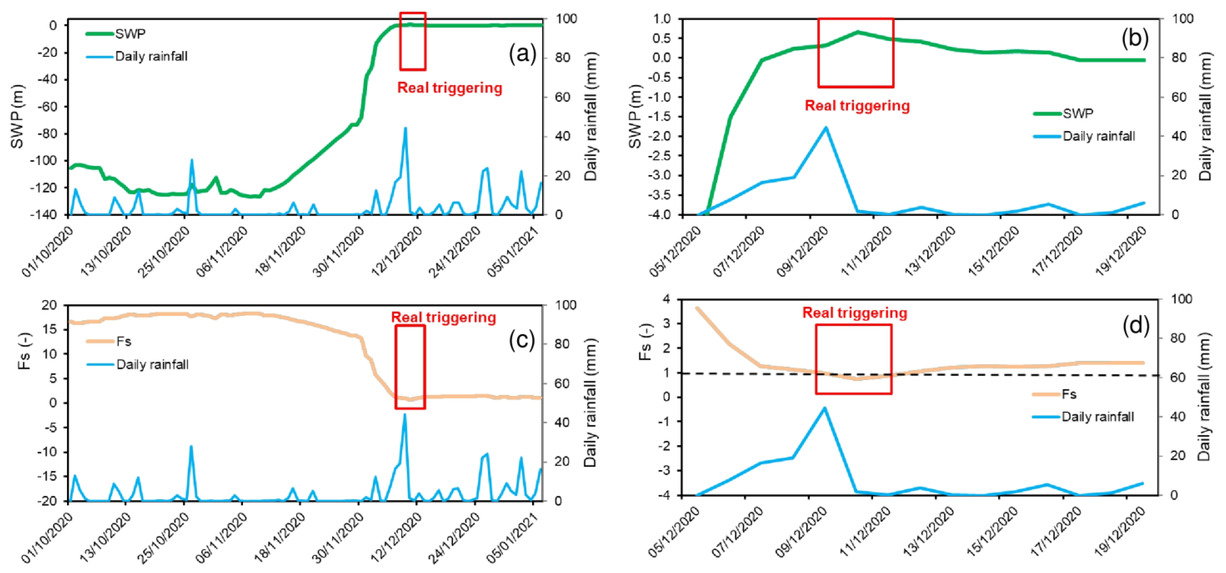
October and November 2020 were dry and quite hot, with few rainfall events, that did not exceed 28 mm/d, and mean daily temperatures between 9.5 and 12.4 °C. The shallow soil kept unsaturated conditions at both the test-sites, as demonstrated by SWP values between −40 and −19 m at 0.6 m at Montuè and between −125 and −82 m at 0.9 m at Costa Cavalieri (
Figure 9a and
Figure 10a).
Instead, since 1 December 2020 up to the end of the considered time span, the weather was significantly wet and cold at both test-sites. A cumulated rainfall of 238.6 and 218.6 mm in December at Montuè and Costa Cavalieri, respectively, was recorded and the average daily temperature was 3.6 °C at Montuè and 2.5 °C at Costa Cavalieri. At both analyzed soil layers, SWP increased quickly between 1 and 4 December 2020, in consequence of a cumulated rainfall of 59 mm in 4 days. SWP reached conditions close to 0 m at both test-sites at the end of this event, with higher values (−0.03 m) at Montuè than those at Costa Cavalieri (−1.5 m), due to the infiltration speed required to reach soil horizons located deeply in the soil profile (
Figure 9a and
Figure 10a).
A further significant rainfall event affected both test-sites between 5 and 6 December 2020. A rainfall of 31.6 mm and 24.8 mm in 2 days was measured at Montuè and Costa Cavalieri, respectively. This rainfall caused another important increase of SWP at both the analyzed layers, with the consequent development of positive pressures (0.13 and 0.24 m at Montuè and at Costa Cavalieri, respectively) on 5 December 2020 (
Figure 9b and
Figure 10b).
Positive values of SWP were not further maintained at 0.6 m at Montuètest-site the following day (6 December), while conditions of complete saturation (SWP = 0.02 m) were kept in Costa Cavalieri at 0.9 m from ground level. Costa Cavalieri area experienced another significant rainfall event during the period 8–10 December 2020, when a rainfall of 65 mm in 51 hwas observed. In the same period, a lower amount of rainfall (32.4 mm) was registered in Montuè area. Thus, following a decrease of about 0.2 m in SWP on 6 December 2020, SWP got a further increase at both test-sites. At Montuè test-site, SWP reached values up to −0.07 m on 10 December 2020, without the development of positive pressures as on 5–6 December, due to the lower average rainfall intensity of the event (1.2 mm/h during 5–6 December, 0.6 mm/h during 8–10 December;
Figure 9b). Instead, at Costa Cavalieri, SWP reached values of 0.66 m on 10 December 2020, representing the peak value of SWP modeled in this site during the analyzed time span (
Figure 10b).
In the period between 11 December 2020–6 January 2021, further rainfall events of intensity between 0.2 and 26.4 mm/d kept the soil in a wet condition at both sites. At Montuè test-site, SWP kept close to saturation, with a continuous oscillation in the range (−0.8; −0.1 m) caused by the alternation of dry days and rainy days with consequent rainwater infiltration (
Figure 9a). A very intense and concentrated rainfall of 46.5 mm/d affected the Montuè area on 25 December 2020. SWP increased 0.7 m for rainwater infiltration, even if no transient positive pressure developed (SWP was initially equal to −0.87 m and became equal to −0.14 m at the end of this event). Instead, positive pressures were maintained at Costa Cavalieri test-site, with an almost steady SWP of 0.11 m in this time span, due to the higher depth (0.9 m) of the observed layer and to the lower evapotranspiration effects caused by a lower air temperature in this test-site (average values of 2.3 °C and 4.2 °C at Costa Cavalieri and Montuè, respectively;
Figure 10a).
Instead, the intense rainfall event occurred on 8–10 December 2020 and provoked an increase in positive SWP at Costa Cavalieri test-site. This condition corresponds to a drop in the modeled factor of safety (Fs) below 1, allowing us to model unstable conditions in those days when shallow landslides were really observed in Costa Cavalieri area (
Figure 10d).
Further unstable conditions (Fs < 1) were not modeled in the remaining days of the analyzed time span, even if Fs kept in the range of (1.1, 1.5) due to SWP conditions identifying close-to-saturation or completely saturated soils (
Figure 9c and
Figure 10c).
The reconstruction of daily Fs demonstrated that the modeled SWP trends could be reliable tools for the appropriate assessment of daily SWP conditions, to be used in slope stability analysis and for the correct identification of real triggering time of shallow landslides.
A further validation of using the modeled SWP trend for the identification of triggering moments of shallow landslides was carried out using the daily values to choose the correct physically-based rainfall threshold for the occurrence of these phenomena (
Figure 11).
The first 64 days in Montuè area and the first 67 days in Costa Cavalieri area of the analyzed time span were characterized by SWP lower than −1 m. For these reasons, the threshold for initial soil condition lower than −1 m of SWP had to be considered (
Figure 11a). The rainy period, which began in the first days of December 2020, caused an increase in SWP to conditions close-to saturation or of complete saturation, which were maintained for the remaining days of the analyzed time span (
Figure 11a). In Montuè area, the threshold for completely saturated soils (SWP of 0 m) had to be chosen in 3 days (4–6 December 2020), while the threshold for initial conditions between −1 and 0 m was selected in 30 days (7 December 2020–6 January 2021). In Costa Cavalieri area, the threshold for completely saturated soils (SWP of 0 m) had to be chosen in 19 days, while the threshold for initial conditions between −1 and 0 m was selected in 14 days. The bigger number of days, when the threshold for completely saturated soils had to be selected, in Costa Cavalieri reflected the higher depth of the potential shallow landslides sliding surface and the lower evapotranspiration effects caused by a lower air temperature in this zone.
The reliability in the selection of the most adapted threshold for each day since the use of the modeled values of SWP was confirmed when the prediction of stable and unstable conditions was carried on. All the rainfall events of the analyzed period, when SWP was between −1 and 0 m at the beginning of the event, felt correctly below the corresponding threshold, since no shallow landslides were triggered in the test-sites in similar conditions during the analyzed time span (
Figure 11b). As regards to the events when SWP was equal to 0 m at the beginning of the rainfall, the two real triggering events occurred in Montuè and Costa Cavalieri during the analyzed time span were located correctly above this threshold, while the other events were placed below it, confirming that no shallow failures occurred during those rainfalls (
Figure 11c).
This analysis confirmed the reliability of the modeled values of daily SWP in both the test-sites and their effective implementation to select the correct rainfall threshold for the possible occurrence of shallow landslides in those areas.
4. Discussion
A data-driven method is proposed to model the temporal trends of SWP at different soil depths and for different geological and geomorphological contexts. This model represents a new and innovative approach for the estimation of this hydrological parameter, which is usually measured in field or estimated by means of physically-based models.
First, different statistical methods were tested to find the best algorithm to be implemented in the estimation model of SWP. Even if all the used methods could guarantee an excellent estimation of real measured temporal trends, the models based on Random Forests performed in the best way, with an outstanding effectiveness (R
2 of 0.98, MAE of (0.11–0.16) m, NS of (0.98–0.99)). The best performance measured for Random Forest was related to the ability of this machine learning technique to reconstruct complex linear and, also, non-linear relationships between the explanatory variables and the response variable of the model. In fact, non-linear hydrological processes occur generally in rainwater infiltration during wet periods and in evapotranspiration during dry days, influencing the distribution of SWP values in time and at different depths [
47].
The Random Forest models, identified as the ones which outscored the real measured trends of SWP, allowed estimation of the effects of different meteorological explanatory variables to SWP temporal trends in test-sites with different geological and geomorphological features, and, for a particular area, at different depths in the soil profile.
Considering silty or silty clay soils as the ones of the analyzed test-sites, the models for the most superficial soil layers (0.6 m from ground level in both the test sites) were more sensitive to short-time span rainfall amounts and air temperatures dynamics. These layers are located closer to the interface with the atmosphere and are affected by the dynamics of rainfall events and air temperature trends occurring at daily resolution or during the few days before a certain date [
7,
40]. Instead, SWP dynamics of the tested soil levels located in a deeper soil profile (0.9 m from ground at Costa Cavalieri, 1.2 m from ground at Montuè) are more influenced by long-term rainfall amounts and air temperature trends. The reasons for these behaviors are linked both to the physical and hydrological features of the tested materials (silty or silty clays soils with medium permeability) and to the larger distance from the interface with atmosphere, which determines a higher time span for the rainwater infiltration and for the air temperature to modify significantly the values of SWP [
21].
The performance of all the selected models improved significantly when considering also the average antecedent values of SWP for 3 and 7 days before a certain date, in correspondence to all the tested soils. This fact testifies how a soil can keep the “memory” of an antecedent hydrological status and can “remember” these conditions after the meteorological conditions that determine this status are forgotten by the atmospheric variables. This particular behavior of a soil layer is more pronounced in fine textural soils [
7,
42,
48], as the one present in the analyzed test-sites and is fundamental to obtain a reliable model to forecast SWP trends along time [
40,
49].
In the selected test-sites, characterized by soils with fine textures, SWP estimation was not impacted significantly by meteorological variables such as atmospheric pressure, air humidity, wind speed and solar radiation, at different depths in the soil profile. In fact, the drop in performance of the models was nil when these meteorological variables are permuted. This observation is consistent with previous studies where data-driven models for the estimation of other soil hydrological parameters (soil water content, depth of the groundwater table) showed a limited or a nil influence of these variables on the predicted trends of the response hydrological variable [
40,
49,
50]. The low influence of these parameters could be due to their lower effect on the evapotranspiration dynamics in the soil than air temperature or previous rain amounts, especially in layers not in correspondence with the atmospheric boundary [
51].
Along the analyzed timespans, the chosen models (RF models) allowed to estimate correctly the temporal trends of SWP in different depths of both test-sites, identifying the variation of hydrological behaviors throughout the different seasons and in relation to dry and wet periods. Thanks to the reliability of these models, SWP trends were reconstructed in an effective way, allowing us to identify the fast response of the most superficial soil layers to rainfall events and to dry periods and, at the same time, the delayed and more seasonal response of the deepest analyzed soil layers to more prolonged rainy and dry periods, due to the effect of the deep rainwater percolation occurring in a longer time period. Furthermore, the modeled SWP trends of both test-sites recognized correctly the moment when nil or positive SWP occurred, testifying the formation of a transient perched groundwater table that has significant influence on soil water dynamics and fluxes and, also, on other soil properties, such as the soil shear strength.
The high predictive capability of the selected machine learning models determined their ability in simulating correctly the trends of SWP along a time period different from the monitoring ones, used to build and test the models themselves. In this particular period (1 October 2020–6 January 2021), both the areas were affected by shallow failures. The modeled SWP trends, in correspondence with the sliding surface of these phenomena (0.6 m from ground at Montuè, 0.9 m from ground at Costa Cavalieri), showed the highest values of the SWP in the days when shallow failures really occurred. The modeled trends of slope factor of safety (Fs) highlighted values below 1 (unstable conditions) only in correspondence of the same days, consistent with the observations of real triggering events.
The reliability of the modeled SWP trends during unstable times is confirmed by the ability of the models to identify different triggering mechanisms, characterizing the modeled shallow landslides events. At depth of 0.6 m at Montuè test-site, a shallow failure triggered in consequence of the development of a transient water table (SWP of (0.13–0.24) m) formed for the downward propagation of the wetting front at the end of six heavy rainy days(91.6 mm of rain in 5 days) [
52]. Instead, at 0.9 m from ground of Costa Cavalieri test-site, a shallow landslide occurred in consequence of the uprising of a perched water table [
31,
52], which developed in 8 days of particularly rainy (83.4 mm in 8 days) weather and upraised during a further intense rainfall event (65 mm of rainfall in 51 h) causing the development of a SWP up to 0.66 m.
Moreover, even if the analyzed test-sites showed an intrinsic proneness to shallow slope failures due to the presence of soils with friction angle close to the slope steepness and nil cohesion, the reconstructed Fs trends highlighted the significant impact of SWP dynamics on the triggering of these phenomena. In particular, the development of positive SWP values can reduce the shear strength of the slope materials leading to the triggering of slope instabilities when limit values of SWP are exceeded.
The application of a simplified model for the slope Fs calculation, based on modeled trends of SWP, could be limited at slope scale or at small catchments, characterized by quite uniform geological, geomorphological and hydrological features [
53]. However, the estimated trends of SWP can be useful for the most appropriate selection of the best rainfall thresholds, validated for the identification of triggering events up to regional scale, within a different set of models obtained from different initial soil conditions in terms of SWP [
54].
As for Fs calculation, the reliability of estimated SWP trends was confirmed since all the rainfall events of the analyzed period, in case of −1 m < SWP < 0 m at the beginning of the event, fell correctly below the corresponding threshold, in fact no shallow landslides were observed at the test-sites. As for the events in the case of SWP = 0 m as initial condition, the two real triggering events occurred in Montuè and Costa Cavalieri during the analyzed time span and were located correctly above this threshold, while the other events were placed below, thus confirming that no shallow failures occurred during those rainfall events.
The developed data-driven methodology represents a new approach for the reconstruction of SWP trend and dynamics in different settings and at different depths of soil profile. This method can allow to fill several gaps of other methodologies for the assessment of SWP dynamics, such as physically based models for slope stability analysis.
Unlike models based on physical-mathematical equations, a data-driven technique does not require the physical and hydrological parameters of the soils as input data, which are sometimes difficult to acquire [
17,
22]. If the model for SWP assessment is reconstructed for a test-site, which can be assumed representative of the whole catchment typical features, the use of meteorological and hydrological predictors map scan allows to apply the model over large areas. Instead, physically-based models are limited in this application due to computational burden and poor availability of a reliable dataset of soil parameters [
53]. The developed methodology allows to obtain reliable results in terms of SWP temporal dynamics, also for periods when real measures of SWP are not available, to carry out the comparison with the modeled trends. As demonstrated in the application of modeled SWP for slope safety factor calculation and for selection of physically-based rainfall thresholds, these trends could allow to obtain accurate datasets of water potential values. These values, in turn, could be useful in implementing other methodologies to estimate specific geological and hydrological processes (e.g., landslides triggering, runoff generation, irrigation scheduling; [
22]).
The models reconstructed in correspondence of a representative test-site of a setting could be used to simulate SWP temporal trends also for other hillslopes or areas which have similar geological and geomorphological features and soils with similar properties to the ones of the representative slope. If datasets or maps of the input predictors of the model are available for areas with similar features to the test-site where the model was reconstructed, SWP daily values and temporal trends could be estimated for wide sectors, obtaining also maps of distribution of this parameter that could be useful for shallow landslides prediction and hazard analysis at large scale.
However, it is necessary to highlight the limits of this methodology for its comprehensive evaluation and possible application in other contexts.
A machine learning model requires a training time with real measured data of soil water potential. This period has to be long enough to consider all the different responses of the soil in various weather conditions. For this reason, possible errors of SWP estimation, in periods when real measured data are not available, could be due to some particular daily or seasonal meteorological conditions that did not exist in the training set of the model [
39]. For particular applications, the model could be developed with time-steps smaller than those use herein (e.g., hours). Thus, it is required to verify if a similar approach is able to produce outstanding results also for finer time resolutions [
55].
5. Conclusions
A new and innovative data-driven method, based on a machine learning technique, was developed and tested for the temporal estimation of soil-water potential trends, at different depths of a soil profile and in different settings. This approach showed that Random Forest models allowed an outstanding reconstruction of the temporal trends of this hydrological parameter, compared to measured-in-field trends. The results showed that meteorological and hydrological characteristics have different effects on soil water potential. The reliability of the models was confirmed when they simulated soil-water potential trends for a different timespan, in particular in the correct estimation of days when shallow landslides were triggered in the study areas by means of a slope stability model and of the appropriate choice of the physically-based thresholds.
Considering its reliability, main advantages, and weak points, the proposed methodology is able to capture temporal variability of soil-water potential in different contexts and has a high capability in simulating complex relationships between meteorological and hydrological predictors and the selected response variable. If both forecasted meteorological forcing and hydrological parameters are incorporated as input data, the models will allow to simulate possible soil-water potential scenarios that could be used for decision-making purposes indifferent fields (e.g., early-warning system for landslides occurrence; agricultural management).
Its flexibility and feasibility make the method potentially applicable to different geological and geomorphological settings characterized by other hydrological and soil features, such as areas with the presence of coarser soils (e.g., sandy soils), where the effects of model predictors on SWP temporal dynamics could be different. Moreover, the availability of meteorological and hydrological predictors maps of the model could allow to calibrate and extend the model to wider areas, in order to obtain a more comprehensive assessment of soil-water potential dynamics at scales wider than the representative test-site slopes.


 ,
, 


