
Phytoplankton Community in the Western South China Sea in Winter and Summer


1
College of Biotechnology, Tianjin University of Science and Technology, Tianjin 300457, China
2
Research Centre for Indian Ocean Ecosystem, Tianjin University of Science and Technology, Tianjin 300457, China
3
College of Marine Science and Technology, China University of Geosciences (Wuhan), Wuhan 430074, China
*
Author to whom correspondence should be addressed.
Water 2021, 13(9), 1209; https://doi.org/10.3390/w13091209
Submission received: 9 February 2021
/
Revised: 5 April 2021
/
Accepted: 9 April 2021
/
Published: 27 April 2021
(This article belongs to the Special Issue Marine Nitrogen Fixation and Phytoplankton Ecology)
Abstract
:Phytoplankton are known as important harbingers of climate change in aquatic ecosystems. Here, the influence of the oceanographic settings on the phytoplankton community structure in the western South China Sea (SCS) was investigated during two seasons, i.e., the winter (December 2006) and summer (August–September, 2007). The phytoplankton community was mainly composed of diatoms (192 taxa), dinoflagellates (109 taxa), and cyanobacteria (4 taxa). The chain-forming diatoms and cyanobacteria Trichodesmium were the dominants throughout the study period. The phytoplankton community structure displayed distinct variation between two seasons, shifting from a diatom-dominated regime in winter to a cyanobacteria-dominated system in summer. The increased abundance of overall phytoplankton and cyanobacteria in the water column during the summer signifies the impact of nutrient advection due to upwelling and enriched eddy activity. That the symbiotic cyanobacteria–diatom (Rhizosolenia–Richelia) association was abundant during the winter signifies the influence of cool temperature. On the contrary, Trichodesmium dominance during the summer implies its tolerance to increased temperature. Overall, the two seasonal variations within the local phytoplankton community in the western SCS could simulate their community shift over the forthcoming climatic conditions.
1. Introduction
The South China Sea (SCS), a typically oligotrophic area, is the largest marginal sea in the tropical Pacific Ocean. The upper SCS is characterized by the monsoon-induced circulation and mesoscale eddies which predominantly impact biogeochemical progress; concurrently, the riverine input from the Pearl and Mekong Rivers dramatically affects nutrient exchange in the SCS [1,2,3,4]. Despite receiving large amounts of terrestrial nutrient input through the riverine discharge, the SCS only utilizes a small portion to support productivity [5,6]. Nutrient concentrations in the SCS are often below the detectable limits [7]. The ratios of nitrogen to soluble reactive phosphorus (N/P) were much lower than 16 (the Redfield N/P Ratio), suggesting nitrogen limitations in the SCS [8]. Nutrient deficiency causes relatively low chlorophyll concentrations [9,10,11], and low phytoplankton stock compared with other adjacent marginal seas [12,13,14]. The western SCS is located towards the east of the Vietnam coast, where the deep basin is extended by steep slopes, with a maximum depth reaching 4000 m. Vietnamese upwelling is one of the typical features in the western SCS, and the Vietnam offshore flowing to the north in summer causes a local enhancement of Vietnamese upwelling intensity [6]. In the western SCS, cyclonic eddies form frequently with a raised thermocline in winter, and anticyclonic eddies form with a depressed thermocline in summer [15]. Besides, summer circulation often has a dipole structure associated with an eastward jet, appearing off central Vietnam [16]. These physical processes control nutrient flux from the deep water into the euphotic zone and subsequently affect the ocean’s ecological status [17].
Marine phytoplankton, as the most important primary producer at the base of the marine food chain, are responsible for generating roughly half of the global net primary production, and play a key role in the elements cycle and energy flow in a marine ecosystem as the primary producers [18]. Physical processes such as upwelling and eddies are particularly relevant to phytoplankton productivity [19]. The instabilities of these processes help to create and maintain localized environments that favor the growth of phytoplankton [17]. The coupling between these physical and biological processes influences phytoplankton biomass and seasonal succession [20]. In the western SCS, a series of physical processes, controlling nutrient flux into the euphotic zone, play a profound role in supporting the phytoplankton growth and their spatio-temporal distribution [21,22,23,24,25,26]. High chlorophyll a concentration often occurs in the western SCS, where phytoplankton blooms even appear in summer when southwest monsoons are parallel to the Vietnamese coast [21,22]. Wang and Tang (2014) observed that the patchiness in spatial and vertical phytoplankton distribution was controlled by the vertical flux of nutrients caused by curl-driven upwelling in the western SCS [23]. Liang et al. (2018) found that the high chlorophyll a belt was determined by the advection of coastal upwelling water by the northeastward jet and the resultant cyclonic/anticyclonic eddies, which were defined as a ‘jet-eddy system’ [27]. Wang et al. (2016) calculated that the contribution of phytoplankton groups to the total chlorophyll a biomass changed along with cyclonic eddy dimensional structure [25].
Many studies have investigated phytoplankton biomass and the coupling of biological–physical processes in the western SCS. These existing related studies were focused mainly on pigments and remote sensing observations. However, yet, quantitative measures of phytoplankton diversity, a comprehensive interpretation of phytoplankton successions, and knowledge of interactions with diverse hydrodynamic settings are still meager. Knowledge of phytoplankton species and their response within the marine environment is essential to understand the responses of ocean biota to a dynamic ecosystem and changing global climate [28]. Here, we carried out a series of biogeochemical investigations during two seasons (winter and summer) in the western SCS. In this study, the cold-core cyclonic eddies and warm-core anticyclonic eddy were observed during the summer investigation [29]. The main objectives of this study were to evaluate the spatial and temporal difference of the phytoplankton community structure in different seasons, aiming to supply a cue of how physicochemical influence on the phytoplankton community shifts, to provide insights into the acclimation and adaptation of the phytoplankton community to a changing marine environment.
2. Materials and Methods
2.1. Study Area
The sampling was carried out from the western SCS extending eastwards from the Vietnamese shelf region towards the eastern deep basin (10–15° N, 110–112.5° E) (Figure 1). In this region, the seasonal reversal of monsoon winds mainly controls the upper-ocean circulations (Shaw and Chao, 1994). During the northeast (or winter) monsoon (November to March) a stronger cyclonic gyre exists in the western portion of the southern SCS [30]. A strong coastal jet occurs in the western boundary of the SCS, southward along the continental shelf from the Chinese coast to southern Vietnam [31], causing the basin-scale circulation. On the contrary, during the southwest (or summer) monsoon (April to August), the weaker anticyclonic gyre dominates upper layer circulations in the southwestern SCS. The northward jet separates from the Vietnamese coast at about 12° N in summer [32] and eddy pairs associate with the jet forms [33]. The upwelling takes place off the Vietnamese coast, which flows northeastward and carries the cold continental water into the open basin [31]. Two cruises were conducted on the R.V. ‘Dongfanghong 2′ during the southwest monsoon (December 2006) and northeast monsoon (August–September, 2007) periods to assess the phytoplankton community structure in the western SCS. Two cyclonic mesoscale cold eddies were monitored in August and September, which were named as cold eddy 1 (CE1) and cold eddy 2 (CE2), respectively, during the cruise using in situ current, hydrographic measurements as well as concurrent satellite altimeter observations [29,34]. With a relatively steady intensity and radius, the CE2 endured for two weeks after its swift formation in late August and prior to its quick dissipation in mid-September. The anticyclonic warm eddies, marked WE, were also observed in the survey area [29]. During this study, a total of 15 and 36 stations were investigated in winter and summer, respectively. The sampling stations marked with dotted circles were located within the eddy area (Figure 1).
2.2. Sample Collection and Analysis
Seawater samples were collected from seven depths (0, 25, 50, 75, 100, 150, and 200 m) at 51 sampling stations using the Niskin bottles attached to a Rosette water sampler fitted with a Seabird 917 Plus site CTD system. A total of 40 and 230 samples for phytoplankton analysis were collected in winter and summer respectively. Temperature and salinity data were derived from the Seabird CTD. For enumeration of the phytoplankton community, a 3 L seawater sample was concentrated to 1 L by using 10 µm mesh and taken into polyethylene (PE) bottles, then fixed with 2% buffered formaldehyde solution and stored in darkness until completing the voyage.
After returning to the laboratory, the Utermöhl method was applied for phytoplankton water sample analysis [36]. A 1 L subsample was stood for 48 h, then 800 mL supernatant was removed carefully by siphoning through a catheter; it was important to note that the position of the catheter avoided touching the bottom of the bottle. After that, the remaining 200 mL liquid was well mixed gently, half of which was further concentrated with a 100 mL sedimentation column (Utermöhl method) for 48 h sedimentation [37]. Then, the phytoplankton species were identified and enumerated under an inverted microscope (AE2000, Motic, Xiamen, China) at 400× (or 200×) magnification, and five enumerations were performed under the non-overlapping field (529 field in total). The size limit of resolution for this analysis was ~5 μm. The phytoplankton species were identified using published standard literature [38] and the World Register of Marine species (http://www.marinespecies.org, Updated: 12 April 2021). The species identification was as close as possible to the species level.
For nutrient estimation, 100 mL of seawater was collected in the clean plastic bottles and stored at −20 °C till further analysis. Nutrition data were supplied by Dr. Min Han Dai’s lab, Xiamen University. In detail, dissolved inorganic nitrogen NOx (NO3 − + NO2−) was analyzed by reducing NO3− to NO NO2− with a Cd column and then determining using the standard pink azo dye method, and a flow injection analyzer [39]. The dissolved inorganic phosphorus (PO43−) concentrations were measured using two independent methods. For PO43− concentrations > 500 nM, the concentration was measured by the standard molybdenum blue procedure [40], and for PO43− concentrations < 500 nM, measurements were taken with a home-made ship-board C18 enrichment-flow injection analysis system [24,41]. Silicate concentrations were estimated using the standard silica aluminum blue spectrophotometry method [39].
2.3. Data Analysis
Horizontal and depth-integrated distribution of phytoplankton and physiochemical parameters were projected using Ocean Data View 4.7.6 (https://odv.awi.de/en/software/, released on 2 March 2018). The histogram, scatter diagram, and box-whisker plots were plotted with Origin (Version 8.5) [42]. The Spearman’s correlation analysis and canonical correspondence analysis (CCA) between assemblages and physicochemical parameters were performed using Past3 software (http://www.canadiancontent.net/tech/download/PAST.html, released on June 2013).
The phytoplankton community diversity was evaluated mainly using the Shannon–Wiener diversity index (H′), Pielou evenness index (J), and dominance index (Y) [43]. The dominant species of phytoplankton was determined by dominance index (Y).
The Shannon–Wiener (S–W) diversity index (H′) was calculated by the equation below:
where Pi is the relative cell abundance of a species, i is the numbers of the i-th species, and S is the numbers of total species in a sample. The evenness index (J) was calculated from H’ using the following formula:
where H’ is the S–W diversity index, and S is the number of the total species in a sample.
The phytoplankton dominance index (Y) was calculated as follows:
where ni is the number of the individual species, N is the total number of all species, and fi is the occurrence frequency of the species in a sample.
Community alpha diversity indices (Shannon–Weiner index H’, and Pielou evenness index J, Species Richness, Simpson, Chaol) were calculated and performed using the ‘vegan’ package by R version 3.6.1. (https://www.r-project.org/, released on 5 July 2019) [44]. The Kruskal–Wallis test was used to compare the abundance differences of phytoplankton groups and diversity indices among defined groups. The two-tailed t-test was used to compare the abundance of phytoplankton groups between different defined groups.
3. Results
3.1. Seasonality in the Environmental Variables
The surface temperature and salinity in the winter ranged from 27.06 to 28.69 °C and from 33.15 to 33.72, respectively. In summer the surface temperature varied from 26.53 to 29.78 °C, whereas surface salinity ranged from 28.86 to 34.14. During this period, two cyclonic eddies were accurately captured throughout the cruise using in situ current and hydrographic measurements as well as the concurrent satellite altimeter observations [29,35]. One cold eddy, CE1, lay in the north region (112° E, 14° N), which lasted from 15 to 31 August. The other cold eddy, CE2, located in the south region (111° E, 12° N), endured for one week (1–8 September). Meanwhile, a warm eddy (WE) was observed near the CE2 (112° E, 10° N) (6–8 September) (Figure 1). During both seasons, the entire study region was divided into the following eddy stages (as adopted by [35]): no eddy stage (NE, in winter (December 2006)), CE1 stage (15–24 August 2007), CE1 relaxation stage (CE1-r, 25 to 31 August 2007), CE2 (1–8 September 2007), and WE (6–8 September 2007). The sampling stations marked with dotted circles were located within the eddy area (Figure 1). The data of various environmental factors during both seasons are given in Table A1. During all stages, the temperature decreased with water depth. The temperature at 50–100 m was relatively high in the WE stage compared with other stages (Table A1). The salinity increased with water depth. The nutrition concentrations also increased with water depth, and they were relatively high in the winter compared with that in the summer (the eddy stages). Among the different cyclonic stages in the summer, the average concentration of inorganic nitrogen (nitrate and nitrite) was almost below 0.2 μmol/L (except in the CE1 stage) in the upper water (0–50 m). However, in the middle water column (50–100 m), the average concentration of inorganic nitrogen, phosphate, and silicate were relatively higher during the CE1 and CE2 stages than during the CE1-r and WE stages.
3.2. Phytoplankton Species Composition in the Study Region
During the winter, a total of 112 phytoplankton taxa belonging to six phyla (Bacillariophyta, Dinophyta, Cyanophyta, Chlorophyta, Haptophyta, and Chrysophyta) and 39 genera were identified in the study region. The phytoplankton community was mainly composed of diatoms with 99 taxa belonging to 29 genera. Among diatoms, Chaetoceros and Rhizosolenia emerged frequently. Species in the genera Bacteriastrum and Coscinodiscus declined evidently. Nine dinoflagellate taxa belonging to six genera were reported during the present study. The frequency of most dinoflagellate species, especially the species belonging to the genera Protoperidinium, Ceratium, Oxytoxum, Amphisolenia, Ornithocercus, Podolampas, and Dinophysis, was decreased in the winter compared to summer. During the winter season, the cyanobacteria group was mainly comprised of Trichodesmium thiebautii, Trichodesmium erythraeum, and the symbiotic cyanobacteria Richelia intracellularis. Among them, T. thiebautii was the most abundant (0.01), although with an extremely low occurrence frequency (0.50) (Table 1). Besides T. thiebautii, the diatom species Thalassionema nitzschioides, Nitzschia spp., Thalassiosira rotula, Navicula spp., and Chaetoceros spp. dominated the species assemblage (Table 1). Species such as Dictyocha fibula and Scenedesmus quadricauda were also observed during the winter (Table 1). The symbiont cyanobacteria R. intracellularis was mainly associated with diatom species such as Guinardia cylindrus, Rhizosolenia styliformis, and Rhizosolenia hebetata. Notably, its association with R. hebetata was more dominant during the winter.
During the summer season, 320 taxa belonging to 148 genera and six phyla (Bacillariophyta, Dinophyta, Cyanophyta, Chlorophyta, Haptophyta, and Chrysophyta) were identified in the southwestern SCS. Among them, diatoms represented 187 taxa belonging to 54 genera and they were more dominant than the dinoflagellates (109 taxa from 22 genera). The phytoplankton community was more diverse in the summer than in the winter. The number of taxa and genera almost increased by a factor of two and three, respectively. Trichodesmium and Chaetoceros were the fpredominant genera in the phytoplankton community. The chain-forming species, including T. thiebautii, T. nitzschioides, T. erythraeum, Chaetoceros dichaeta, Chaetoceros affinis, Chaetoceros lorenzianus, Thalassionema frauenfeldii, Pseudo-nitzschia delicatissima, Pseudo-nitzschia pungens, Leptocylindrus danicus, Hemiaulus hauckii, and Bacteriastrum comosum, dominated the phytoplankton assemblage during the summer season (Table 1). In addition, the small-sized diatoms Nitzschia spp. and Navicula spp. were widely distributed in the study area. The cyanobacteria species T. thiebautii, T. erythraeum, and symbiotic cyanobacteria R. intracellularis and Calothrix rhizosoleniae were also reported during the summer. R. intracellularis was mainly associated with the diatom hosts such as R. styliformis, G. cylindrus, R. hebetata, and Hemiaulus membranaceus in the intercellular location. However, C. rhizosoleniae was attached externally to species like Chaetoceros subsecumdus, C. affinis, Chaetoceros compressus, Chaetoceros glandazii, and Chaetoceros tortissimus.
3.3. Seasonal Distribution of Phytoplankton Community
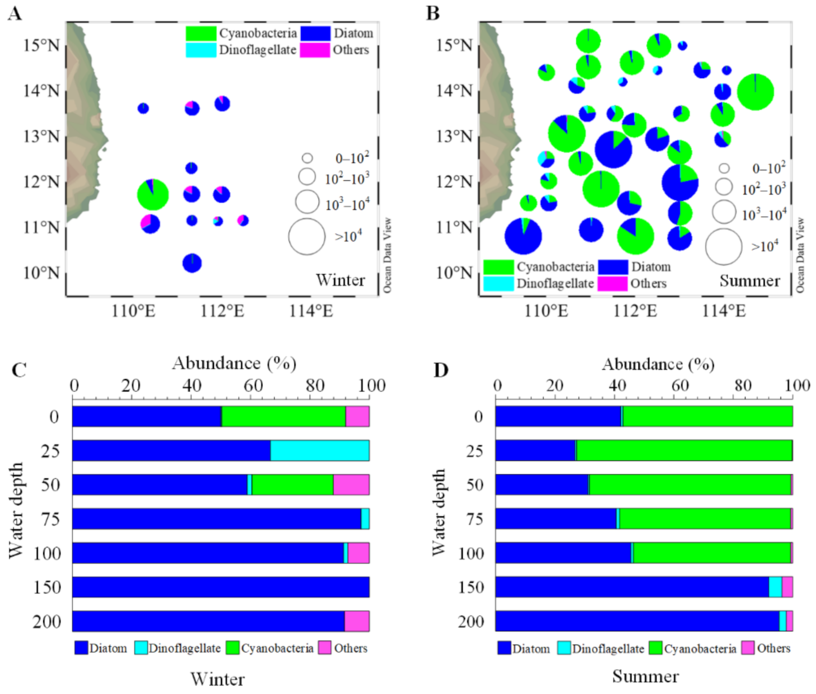
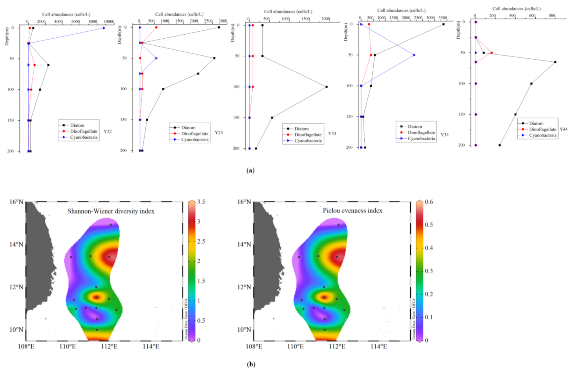
The phytoplankton abundance during the winter ranged from 0.08 × 10³ to 9.52 × 10³ cells L−1, with an average of 2.74 × 10³ cells L−1. Diatom abundance ranged from 0.08 × 10³ to 3.36 × 10³ cells L−1 (average 0.67 × 10³ cells L−1) and comprised ~63% of the total phytoplankton abundance (Table A2). Chaetoceros was a common genus in the diatom group with an average abundance of 0.61 × 10³ cells L−1. Diatoms dominated the phytoplankton assemblage at most stations, except St. Y22, where Trichodesmium contributed 92% (total 8.8 × 10³ cells L−1) to total phytoplankton abundance in the surface water (Figure 2a). Cyanobacteria were observed only in three stations, with the abundance of 0.56 × 10³ cells L−1 at St. Y23, 2.16 × 10³ cells L−1 at St. Y34, and 8.80 × 10³ cells L−1 at St. Y22 (continental region) (Figure A1). Moreover, the total abundance of T. thiebautii was 10.16 × 10³ cells L−1, which accounted for a 24% proportion of the whole community. The symbiotic cyanobacteria only consisted of Richelia intracellularis, with a total abundance of 1.36 × 10³ cells L−1, contributing ~27% to total community abundance. Dinoflagellate abundance ranged from 0.08 × 10³ to 0.16 × 10³ cells L−1 (average 0.10 × 10³ cells L−1) and contributed approximately 1% to total phytoplankton abundance. The highest dinoflagellate abundance was observed at open water station M07 (Figure 2a).
On the contrary, the overall phytoplankton abundance ranged from 0.02 × 10³ to 128.82 × 10³ cells L−1, with an average of 1.05 × 10³ cells L−1. Compared to the winter season, the overall proportion of diatoms in the phytoplankton community decreased by 33.78% in summer, although the ratio of diatom/dinoflagellate was comparable. Conversely, the proportion of cyanobacteria increased by 12.11%, where Trichodesmium contributed up to 44.84% (Figure 2b). The diatom–diazotrophic associations decreased by 2.70%. Cyanobacteria was the most abundant group, as the abundance ranged from 0.02 × 10³ to 123.15 × 10³ cells L−1 (average 1.89 × 10³ cells L−1) and contributed to 69% of the total phytoplankton abundance. The abundance of T. thiebautii reached up to 121.55 × 10³ cells L−1. The total abundance of symbiotic cyanobacteria in the region was 3.36 × 10³ cells L−1, with a Richelia intracellularis and Calothrix rhizosoleniae abundance of 2.20 × 10³ and 1.16 × 10³ cells L−1, respectively. The cyanobacterial population was even distributed in deeper waters in the summer than that in the winter. The average abundance (0.83 × 10³ cells L−1) and the proportion of diatoms were about half that of cyanobacteria (Table A2). Among the diatoms, Chaetoceros was the most dominant species and contributed ~42% to diatom abundance. Dinoflagellates, together with other groups, contributed a small proportion (below 10%) of the phytoplankton community (Table A2). Compared with historical data of phytoplankton composition and abundance in similar regions and seasons, we detected a relatively higher species number in the summer, and the average abundance of phytoplankton was in accordance with previous data (Table 2).
3.4. Vertical Distribution of Phytoplankton Community at Different Eddy Stages
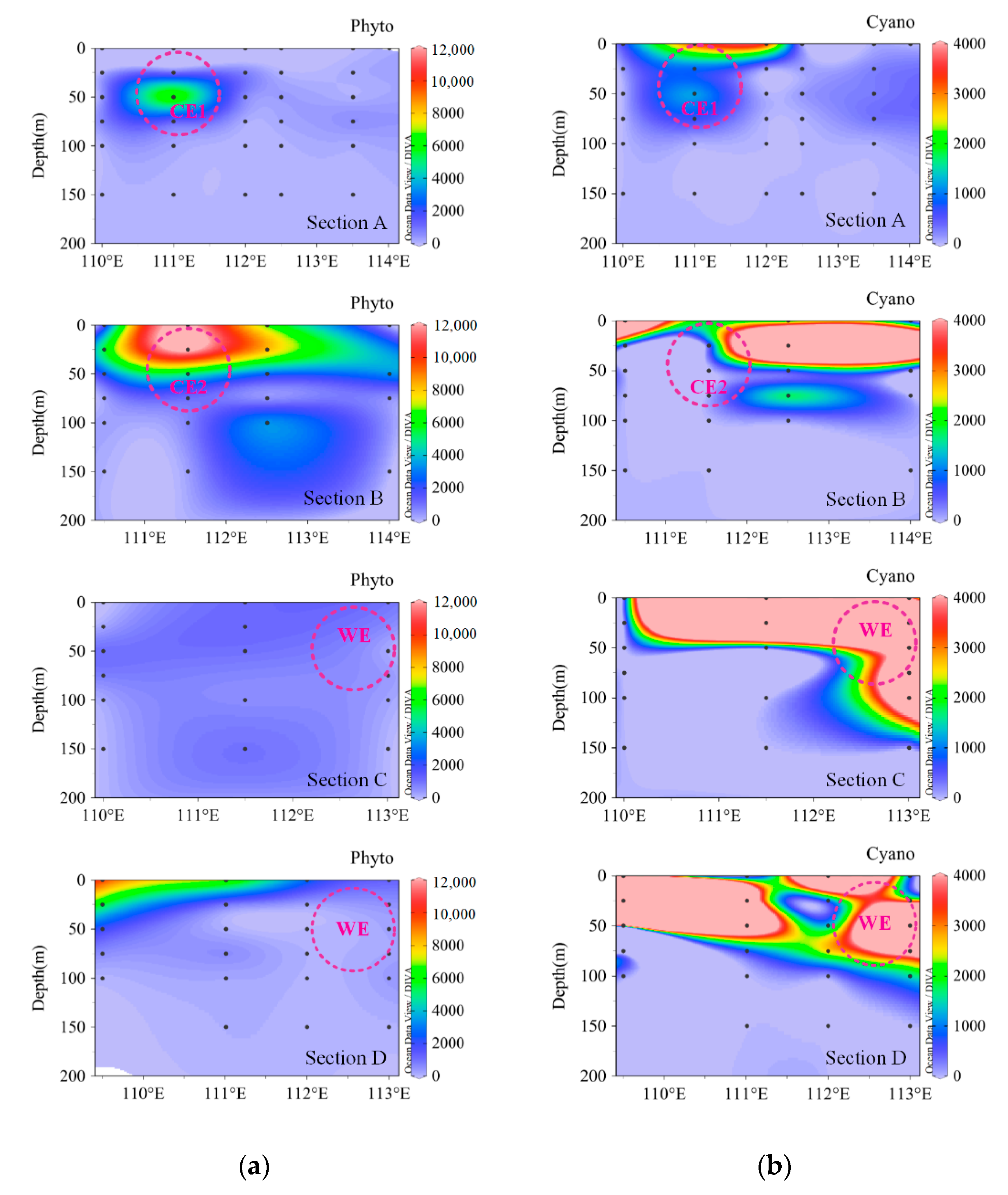
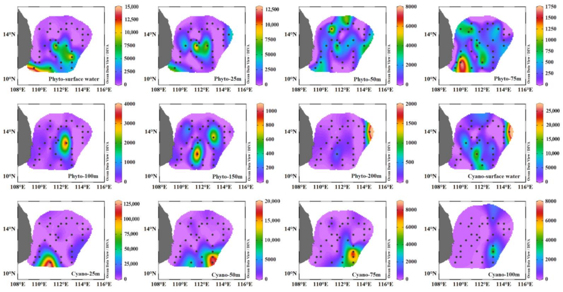
The phytoplankton composition and abundance during the summer and winter seasons were not only different in the surface layer but also the water column (Figure 2). In the winter, the abundances and proportions of cyanobacteria were comparable to that of diatoms, whereas in the summer, the cyanobacterial population was close to double that of diatoms. During the winter, the relative abundance of diatoms was greater below 50 m (peak abundance 2.56 × 10³ cells L−1 at Stn 23), whereas the dinoflagellates (25 m) and cyanobacteria (0 and 25 m) abundance increased above 50 m (Figure 2c and Figure A1). The highest abundance of cyanobacteria (8.8 × 10³ cells L−1) was observed in the surface water at Stn 22. Dinoflagellates contributed more to total phytoplankton at M07. Other phytoplankton species, mainly Dictyocha fibula, were relatively abundant and contributed 7.95% to total phytoplankton abundance in the surface water. During the summer, phytoplankton were mainly distributed towards the south of 13° N. Among them, the cyanobacteria mainly flourished in the area with eddy existence (especially around the sites of 14.5° N, 112° E and 12° N, 114° E), while diatoms were distributed in the southern area and the open basin (Figure 2b, Figure A2). The abundances of diatoms and dinoflagellates in the eddy mature stage (CE2) rose to 10 times that in the eddy relaxation stage (Figure 2b). Dinoflagellates accounted for a relatively high proportion of total phytoplankton at Y00 and stations along 14° N (Figure 2a). The abundance of Dictyocha fibula was very low, with the proportion of 0.06% of total phytoplankton abundance. Overall, depth-wise the cyanobacterial population was relatively abundant (>50%) until 100 m, whereas diatoms and (to some extent) dinoflagellates dominated deeper layers (Table A3). Moreover, the vertical distribution of cyanobacteria revealed their dominance on the edge of cold eddies and the open basin (Figure 3b, Section A, and Section B), as well as in the area influenced by the warm eddy (Figure 3b, Section C, and Section D). Differently, other phytoplankton (excluding cyanobacteria) mainly emerged in the center of cold eddies (Figure 3a, Section A, and Section B), followed by the continental area impacted by coastal upwelling (Figure 3a, Section D).
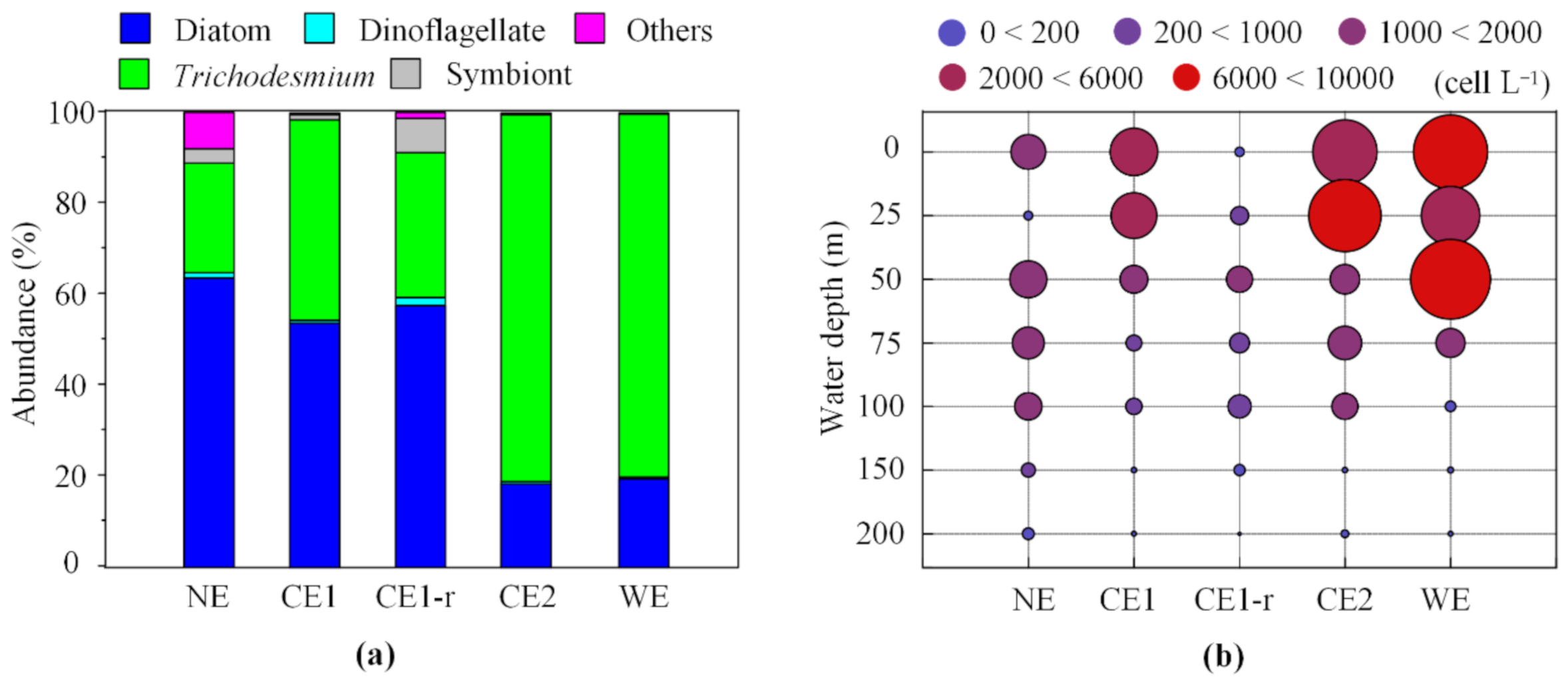
The proportions of the main phytoplankton groups changed remarkably with different stages (Figure 4a). The abundance of Trichodesmium in the phytoplankton community increased in the summer. The ratio of diatom to dinoflagellate (dia/din) was comparable during the winter and summer, whereas it was lower in CE2 (34.10) than in WE (Table A4). The diatom to cyanobacteria ratio (dia/cya) in the winter was five times more than in the summer. Furthermore, the dia/cya ratio was lower in the eddy periods than the no eddy and eddy relaxation stages. The relative contribution of algae groups including diatoms, dinoflagellates, and symbionts decreased dramatically during cold eddy mature stages but increased significantly during the later stages (Figure 4a). The dominant genus Trichodesmium presented a discrepant occurrence; however, its relative contribution to the phytoplankton community was much higher than that in non-eddy stages. The proportion of Trichodesmium (80.92%) and the dia/cya ratio (0.23) in the cold eddy mature period (CE2) were comparable to that in the warm eddy period (WE) (80.06%, 0.24, respectively) (Figure 4a). The phytoplankton abundance varied significantly above 50 m in the water column, while no significant difference was observed below the 50 m layer (Figure 4b). The phytoplankton community significantly varied seasonally (two-tailed t-test, p < 0.05) (Table A5). Similarly, the variation of diatoms and dinoflagellates other than cyanobacteria showed a significant difference between eddy stages (p < 0.01). Moreover, the abundance of different phytoplankton groups, excluding cyanobacteria, had statistical differences among different periods (Kruskal–Wallis test, p < 0.01) (Figure A3). Thus, the overall results indicate that the phytoplankton community composition and structure changed with season and eddy development.
3.5. Diversity of Phytoplankton Community
The Shannon–Weiner index (H’) and Pielou evenness index (J) were used for analyzing phytoplankton community diversity in this study. Our results show that the Shannon–Weiner index had a similar distribution pattern to the Pielou evenness index in both seasons (Figure A1). During the winter, the Shannon–Weiner index and Pielou evenness index ranged from 0.50 to 3.35 (avg. 1.28) and 0.09 to 0.57 (avg. 0.22), respectively, in the surface water (Figure 5a). High phytoplankton community diversity was observed in the open ocean region (Figure 5b). In the summer, the Shannon–Weiner and Pielou evenness indexes ranged from 0.01 to 5.14 (avg. 2.70) and 0.01 to 0.62 (avg. 0.32), respectively, in the surface water. Diversity indices were significantly higher in the summer than winter (p < 0.001), whereas the Pielou evenness index was significantly lower (p < 0.05) during the summer (Figure A1 and Figure A4). This emphasizes that the surface water phytoplankton community in the summer was significantly more diverse than in the winter. Moreover, the phytoplankton community diversity in the summer was high in the water column (from 25 to 75 m depth) and also in eddy-controlled areas. Then, phytoplankton diversity was also higher towards the southern part around 13° N (Figure 5). In the study region, the diatoms and cyanobacteria controlled the phytoplankton community structure, whereas dinoflagellates and other groups contributed significantly to the transformation of the phytoplankton community and diversity.
3.6. Effect of the Environmental Cues on the Phytoplankton Community
The influence of the environmental factors on shaping the phytoplankton community structure in the western SCS was assessed using Spearman’s correlation and CCA analysis (Figure 6). The phytoplankton community in the region was significantly influenced by the seasonality in the environmental characteristics. During the winter season, phytoplankton was positively correlated with temperature and Si/N ratio, and was mainly influenced by nitrogen (nitrate and nitrite) (Figure 6a,b). The various diatom groups had a different response to the aquatic environment. Bacteriastrum and Chaetoceros, which belong to the class of Centricae, exhibited significant relationships with environmental parameters, whereas diatoms that belonged to the class Pennatae had no significant relationship with any environmental parameter (Figure 6a,b). In detail, Centricae was positively influenced by temperature but negatively by water depth. However, Pennatae showed a discrepant relationship with the environment as compared to Centricae. These disparate responses evidence that the Centricae thrives in upper warm water, whereas Pennatae prefers the cool lower water. The Chrysophyte member Dictyocha was significantly associated with the various environmental parameters, which could eventually fuel its growth during the winter (Figure 6a). Cyanobacteria were significantly influenced by N/P and Si/N ratios, while dinoflagellates did not reveal an obvious correlation with environmental parameters.
The abundance of phytoplankton groups, excluding cyanobacteria, was significantly different during both the summer and winter seasons (Kruskal–Wallis test, p < 0.01) (Table A3). During the summer, the various phytoplankton groups (except Pennatae diatoms) were significantly influenced by the changing environmental factors (such as temperature, salinity, and nutrients at the respective depths) (Figure 6c,d)). However, the Pennatae diatom species did not show a significant relationship with environmental parameters, similar to that in winter (Figure 6c,d). Unexpectedly, Dictyocha also was not influenced by the changing water characteristics in the summer season. Cyanobacteria, including Trichodesmium and symbionts, were significantly influenced by the spatially and temporally changing environmental parameters. In summer, temperature, salinity, and nutrients were the important factors significantly controlling the phytoplankton growth (p < 0.05). This could evidence that the dynamic change in the environment (due to eddies and upwelling) results in temperature and nutrient variations, which in turn influence profoundly the phytoplankton community structure.
4. Discussion
4.1. Influence of Hydrological Processes on the Phytoplankton Community
The East Asian monsoon system has a strong bearing on the oceanographic and resultant biological features of the SCS. During the winter monsoons, the circulation in the southern SCS forms a cyclonic gyre, and an anticyclonic gyre during the summer monsoon. The surface water in most areas of the SCS is impoverished of nutrients due to a strong pycnocline, leading to a paucity of phytoplankton stock and production [19]. In winter, towards the western boundary of the SCS, the Vietnam offshore flow (which exists between 11° and 16° N) drifts northwards (along the coast) in the summer and southwards during the winter [31]. This flow pattern forms an offshore jet between 12°–13° N, resulting in a local enhancement of the upwelling intensity during the summer. The peculiarity of stretching deformation separates the Vietnamese upwelling from the offshore area and water masses [6,36]. Simultaneously, a strong coastal jet forms a dipole recirculation pattern and flows northeastward between a cyclonic cold eddy (CE2) and an anticyclonic warm eddy (WE) [29]. In this study, the phytoplankton community, especially diatoms, showed relatively high diversity in the continental margin influenced by the Vietnamese upwelling. Previously, the high Chlorophyll a concentrations were observed along the Vietnamese coast [21,27,51]. Loick-Wilde et al. (2017) estimated that the diatoms dominated the cell-carbon biomass in the Vietnamese upwelling area [11]. The nutrient advection during the coastal upwelling stimulates the phytoplankton growth in the upper layers [27].
During the summer season, eddies were persistent in the upper ocean layers in the SCS. The phytoplankton community structure changed with eddy developments. Statistical analysis revealed that the growth of various algae groups (except cyanobacteria) significantly varied with different eddy development phases, suggesting a significant influence of eddies on the phytoplankton community in the study region. The high phytoplankton abundance observed between the 25 and 100 m depth layers was mainly influenced by eddies. Earlier studies in the SCS pointed out that the maximum chlorophyll a concentration often appeared from 50 to 100 m in the non-eddy region, and appeared at 75 m in the eddy [23,27]. The cold eddy occurrence resulted in a continuous increase in diatom abundance compared to the non-eddy period, as observed previously [20]. The nutrient advection due to variable vertical motion could support the difference in phytoplankton abundance variation in the subsurface water [27]. Mesoscale eddies were proved to supply 20–40% of the nutrient requirements of phytoplankton [52,53]. The enhanced productivity in eddies could be even comparable to the productivity supported by upwelled subsurface nitrate driven during the prevailing monsoon [9]. The increased chlorophyll a concentrations due to nutrient enrichment during cyclonic eddies were also observed elsewhere [54]. Nutrient supplements derived from eddy occurrence, resulting in phytoplankton development, reflected the inter-coupling between physical and biochemical processes in the SCS region.
Different phytoplankton functional groups have a varied response to seasonal and spatial fluctuations of environmental factors [55]. Diatoms are a major starter of food chains and food webs, and important contributors to marine primary production and the ocean carbon cycle [56,57]. Cyanobacteria could maintain the balance of the global ocean nitrogen budget by biological nitrogen fixation [58]. In this study, the diversity and abundance of phytoplankton were much higher in the summer than that in the winter. Diatoms contributed more to phytoplankton abundance in the winter, but cyanobacteria (Trichodesmium dominance) contributed more in the summer. This seasonal variation clearly explains the shifts within the phytoplankton community from diatoms (in winter) to cyanobacteria (in summer). Earlier, in the SCS, a higher proportion of diatoms in the phytoplankton assemblage was reported during the winter than in summer [19]. However, discrepantly, the dominance of Trichodesmium was not reported earlier [19]. Moreover, high phytoplankton abundance was reported at a deeper layer due to the deepened thermocline in the summer, compared with that in the winter. The variations of major phytoplankton groups were explained by different adaptive strategies to overcome the constraints imposed by temperature and nutrient concentration variations in the SCS [59]. Here, wind pumping also played a significant role in inducing high biological productivity during the summer monsoon. The upwelling and cold eddies both fueled the nutrient enrichment and eventually the phytoplankton diversity during the summer season. Overall, in the western SCS, the seasonality of the phytoplankton community and growth dynamics could be significantly influenced by the coupled physical processes mostly driven by the East Asian Monsoon. Changes in compositions of phytoplankton in this study provide clues in understanding the mechanisms that regulate their acclimation and adaptation to changing environments.
4.2. Significance of Diazotrophic Cyanobacteria in the Western SCS
Nitrogen acted as an essential but limiting factor for phytoplankton. Nitrogen concentration in the surface water was mostly below the detection limit in the western SCS. Although frequent eddies, driven by upwelling and monsoon, replenish nutrients from the deeper water, nitrogen lost through denitrification (leading to Redfield ratios below 16) in the water column becomes a major limiting factor for phytoplankton growth [60]. Therefore, diazotrophic cyanobacteria essentially alleviate nitrogen limitation and are involved in regulating marine productivity [1,61,62]. In this study, diazotrophic cyanobacteria containing Trichodesmium and the diatom-associated symbionts Richelia and Calothrix were the highest in abundance. Trichodesmium was the most dominant species in the phytoplankton community in the continental margin and the oligotrophic basin during both seasons. The dominance of Trichodesmium was also recorded in the SCS earlier [62]. The high abundance of Trichodesmium that appeared in the subsurface water could be controlled by upwelling and eddies. Together with eddy perturbations, the abundance of Trichodesmium was more than 12 times higher in the eddy mature period than that in the degenerating stage. Compared to the previous study [19], the Trichodesmium abundance was above one order of magnitude higher in our study. Here, temperature and nutrient concentration were significant influencing factors for the Trichodesmium population. Earlier studies in this region indicated that Trichodesmium regulated the higher N2 fixation and primary production rates in the oligotrophic offshore waters [11]. The nitrogen-fixing by Trichodesmium was quickly converted to plankton biomass and, in particular, the abundance of the diatoms (increased by 1.4–15 factor) in the Pacific Ocean [63]. Thus, here, it can be speculated that the thriving Trichodesmium population potentially contributes the bioavailable nitrogen into the oligotrophic waters in the western SCS. In addition, the symbionts Calothrix and Richelia, and their host diatoms, were relatively abundant in the summer, whereas Rhizosolenia–Richelia dominated in the winter. Symbionts often formed blooms in the low-nutrient water of the Pacific and the Atlantic Oceans [64,65,66,67]. Foster et al. (2011) estimated that the diatom partners influenced the growth and metabolism of their cyanobacterial symbionts Richelia and Calothrix, and the export of diazotroph-derived nitrogen supported the growth of the diatom partners [68]. Thus, diazotrophic symbioses and Trichodesmium would potentially play an important role in the nitrogen supplementation and phytoplankton growth of the oligotrophic ocean.
4.3. Phytoplankton Thermal Adaptations Inferred from Seasonal Successions
Global warming has increased steadily and increasingly involved deeper layers of the ocean since 1990 [69]. The warming ocean temperature would cause an alteration in the succession of the phytoplankton community [70,71,72]. Rising temperatures this century will cause poleward shifts in species’ thermal niches [73]. Concomitantly, the ongoing global climate change is also linked to prolonged periods of anomalously high sea surface temperatures, which are defined as marine heatwaves [74]. From 1925 to 2016, the global average marine heatwave frequency and duration increased by 34 and 17%, respectively, resulting in a 54% increase in annual marine heatwave days globally [75]. Marine heatwaves have been accompanied by a large-scale change in surface chlorophyll levels, shifts in marine species location, and the reshaping of community structure [76,77]. Evidence from the field indicates temperature changes may lead to changes in diatom biogeography [59,78], and each species, even within the same genus, has its own characteristic temperature performance curve [79]. In this study, the seasonal succession of phytoplankton showed a predominance of diatoms in the phytoplankton community in the cool winter, which further shifted to cyanobacterial prevalence during the warm summer. Furthermore, in this study diatoms belonging to Centricae (represented by Chaetoceros, Rhizosolenia, and Bacteriastrum) were significantly related to temperature, as compared to Pennatae groups (such as Fragilariaceae, Naviculaceae, and Nitzschiaceae). The dominance of Centricae diatom species is often observed in the tropical ocean [14,80,81]. In the future, Centricae will become a potentially more sensitive group in the succession of the phytoplankton community as a consequence of the ocean temperature rise. On the other side, ocean stratification caused by rising temperature could result in nutrient deficiency [82]. Cyanobacteria prefer such a warm habitat with the low-nutrient oligotrophic condition. Here, in this study, the declining diatom predominance in the phytoplankton community during the warm condition could reveal their vulnerability to increasing temperature. On the contrary, flourishing cyanobacterial populations, mainly Trichodesmium, in warm conditions reflected their preference and adaptability in response to environmental change. The overall findings of our study could provide insight into phytoplankton community succession in future global temperature rise, and its further influence on biogeochemical cycles.
5. Conclusions
Here, we addressed the seasonal variability of the phytoplankton population in the western SCS, during the summer and winter monsoon periods. The seasonal changes of the phytoplankton community shifted from a diatom-dominated regime in winter to a cyanobacteria-dominated regime in the summer. This community change was controlled by eddies and upwelling activities during this season. Precisely, nutrient advection due to eddy activity triggered phytoplankton abundance, diversity, and Trichodesmium proliferation in summer. However, elevated temperature adversely influenced the diatom–diazotrophic association during the summer. The phytoplankton community succession responses to local oceanographic forces provide insights into forecasting biotic community evolution in the future global climate change.
Author Contributions
Conceptualization, J.S. and C.D.; methodology, J.S.; software, C.D.; validation, J.S. and C.D.; formal analysis, C.D.; investigation, C.D.; resources, J.S.; data curation, J.S.; writing—original draft preparation, C.D.; writing—review and editing, J.S., D.D.N., and H.L.; visualization, C.D.; supervision, J.S.; project administration, J.S.; funding acquisition, J.S. All authors have read and agreed to the published version of the manuscript.
Funding
This research was funded by the National Key Research and Development Project of China (2019YFC1407805), the National Natural Science Foundation of China (41876134, 41676112, 41276124, and 41406155), the Key Project of Key Laboratory of Integrated Marine Monitoring and Applied Technologies for Harmful Algal Blooms (MATHAB201805), the Tianjin 131 Innovation Team Program (20180314), and the Changjiang Scholar Program of Chinese Ministry of Education (T2014253) to Jun Sun.
Institutional Review Board Statement
Not applicable.
Informed Consent Statement
Not applicable.
Data Availability Statement
The data presented in this study are available in insert article.
Acknowledgments
We would like to thank Minhan Dai from Xiamen University for the nutrients data and CTD data supply. Special thanks to Qingshan Luan and Qing He for their hard work in sample collection.
Conflicts of Interest
The authors declare no conflict of interest.
Appendix A

Table A1.
The average of environmental factors during different eddy developmental stages (-: missing data).
Table A1.
The average of environmental factors during different eddy developmental stages (-: missing data).
| Stage | Layer | Temperature (°C) | Salinity | NOx (μmol/L) | PO43− (μmol/L) | SiO32− (μmol/L) |
|---|---|---|---|---|---|---|
| Winter/NE | 0–50 | 27.61 | 33.48 | <0.2 | 0.03 | 2.39 |
| 50–100 | 21.11 | 34.35 | 7.2 | 0.44 | 8.52 | |
| 100–150 | 16.92 | 34.54 | 15.62 | 1.02 | 18.06 | |
| 150–200 | 15.20 | 34.50 | 18.42 | 1.28 | 23.63 | |
| CE1 | 0–50 | 27.55 | 33.77 | 0.50 | 0.05 | 2.70 |
| 50–100 | 22.27 | 34.28 | 5.87 | 0.40 | 7.75 | |
| 100–150 | 17.71 | 34.53 | 14.45 | 0.97 | 15.52 | |
| 150–200 | 13.64 | 34.51 | 15.67 | 1.33 | 24.67 | |
| CE1-r | 0–50 | 27.56 | 33.80 | <0.2 | 0.05 | 2.20 |
| 50–100 | 22.38 | 34.27 | 4.55 | 0.33 | 6.28 | |
| 100–150 | 18.94 | 34.50 | 11.05 | 0.83 | 13.32 | |
| 150–200 | 17.38 | 34.57 | 15.60 | 1.24 | 22.71 | |
| CE2 | 0–50 | 28.36 | 33.37 | <0.2 | 0.03 | 2.28 |
| 50–100 | 22.36 | 34.29 | 6.44 | 0.40 | 7.34 | |
| 100–150 | 17.31 | 34.53 | 14.39 | 0.94 | 14.16 | |
| 150–200 | - | - | 18.80 | 1.27 | 22.19 | |
| WE | 0–50 | 29.18 | 32.99 | <0.2 | 0.05 | 2.25 |
| 50–100 | 24.92 | 33.93 | 4.55 | 0.17 | 3.96 | |
| 100–150 | 17.74 | 34.55 | 14.72 | 0.86 | 13.47 | |
| 150–200 | - | - | 17.50 | 1.11 | 18.16 |
Table A2.
The abundance of phytoplankton during the winter and summer seasons (cell L−1).
| Group | Winter | Summer |
|---|---|---|
| Diatom Range | 80–3360 | 5–13,482 |
| Average | 670 | 827 |
| Total | 26,800 | 190,045 |
| Proportion | 63.57% | 30.18% |
| Dinoflagellate Range | 80–160 | 2–245 |
| Average | 12 | 16 |
| Total | 480 | 3585 |
| Proportion | 1.14% | 0.57% |
| Cyanobacteria Range | 560–8800 | 16–123,150 |
| Average | 288 | 1891 |
| Total | 11,520 | 434,912 |
| Proportion | 27.32% | 69.07% |
| Others Range | 80–560 | 3–60 |
| Average | 84 | 5 |
| Total | 3360 | 1166 |
| Proportion | 8.00% | 0.19% |
| Phytoplankton Range | 80–9520 | 20–128,820 |
| Average | 1054 | 2738 |
| Total | 42,160 | 629,708 |
Table A3.
The in-depth average abundances and proportions of phytoplankton groups during the winter and summer seasons.
Table A3.
The in-depth average abundances and proportions of phytoplankton groups during the winter and summer seasons.
| Season | Depth (m) | Diatom | Dinoflagellate | Cyanobacteria | Others | Total | ||||
|---|---|---|---|---|---|---|---|---|---|---|
| Average (cell L−1) | Proportion | Average (cell L−1) | Proportion | Average (cell L−1) | Proportion | Average (cell L−1) | Proportion | Average (cell L−1) | ||
| Winter | 0 | 704 | 50.00% | 5.33 | 0.38% | 586.67 | 41.67% | 112 | 7.95% | 1408 |
| 25 | 53.33 | 66.67% | 26.67 | 33.33% | 0 | 0 | 0 | 0 | 80 | |
| 50 | 880 | 51.16% | 0 | 0 | 680 | 39.53% | 160 | 9.30% | 1720 | |
| 75 | 1706.67 | 86.49% | 80 | 4.05% | 0 | 0 | 186.67 | 9.46% | 1973.33 | |
| 100 | 1008 | 91.30% | 16 | 1.45% | 0 | 0 | 80 | 7.25% | 1104 | |
| 150 | 304 | 100% | 0 | 0 | 0 | 0 | 0 | 0 | 304 | |
| 200 | 176 | 91.67% | 0 | 0 | 0 | 0 | 16 | 8.33% | 192 | |
| Summer | 0 | 1978.19 | 38.02% | 39.14 | 0.75% | 3182.31 | 61.16% | 3.04 | 0.06% | 5202.69 |
| 25 | 1372.29 | 17.06% | 32.58 | 0.40% | 6633.21 | 82.45% | 6.50 | 0.08% | 8044.56 | |
| 50 | 1295.67 | 41.45% | 13.52 | 0.43% | 1803.94 | 57.71% | 13.10 | 0.42% | 3126.23 | |
| 75 | 414.11 | 31.61% | 10.49 | 0.80% | 880.32 | 67.20% | 5.42 | 0.41% | 1310.35 | |
| 100 | 264.39 | 43.48% | 4.90 | 0.81% | 335.40 | 55.17% | 3.68 | 0.61% | 608.39 | |
| 150 | 125.54 | 95.84% | 3.17 | 2.42% | 0 | 0 | 2.08 | 1.58% | 130.79 | |
| 200 | 107.60 | 97.82% | 1.23 | 1.12% | 0 | 0 | 1.09 | 0.99% | 109.92 | |
Table A4.
TThe abundance of phytoplankton groups at different eddy developmental stages.
| Group | NE | CE1 | CE1-r | CE2 | WE | |
|---|---|---|---|---|---|---|
| Abundance (cell L−1) | Diatoms | 26,800 | 104,334 | 3654 | 53,827 | 28,231 |
| Dinoflagellate | 480 | 1258 | 116 | 1579 | 627 | |
| Cyanobacteria | 11,520 | 87,816 | 2507 | 236,753 | 116,098 | |
| Trichodesmium | 10,160 | 85,635 | 2025 | 236,341 | 115,810 | |
| R. intracellularis | 1360 | 2181 | 482 | 411 | 288 | |
| Other groups | 3360 | 621 | 82 | 406 | 56 | |
| Total | 42,160 | 194,029 | 6359 | 292,564 | 145,012 | |
| Proportion | Diatoms | 63.57% | 53.77% | 57.46% | 18.40% | 19.47% |
| Dinoflagellate | 1.14% | 0.65% | 1.82% | 0.54% | 0.43% | |
| Cyanobacteria | 27.32% | 45.26% | 39.42% | 80.92% | 80.06% | |
| Trichodesmium | 24.10% | 44.14% | 31.84% | 80.78% | 79.86% | |
| R. intracellularis | 3.23% | 1.12% | 7.58% | 0.14% | 0.20% | |
| Other groups | 7.97% | 0.32% | 1.29% | 0.14% | 0.04% | |
| Abundance ratio | Diatoms/Dinoflagellate | 55.83 | 82.94 | 31.50 | 34.10 | 44.99 |
| Diatoms/Cyanobacteris | 2.33 | 1.19 | 1.46 | 0.23 | 0.24 | |
Table A5.
The average abundances of phytoplankton groups were analyzed by t-test between different eddy developmental stages.
Table A5.
The average abundances of phytoplankton groups were analyzed by t-test between different eddy developmental stages.
| Winter | CE1 | CE1-r | CE2 | |
|---|---|---|---|---|
| Summer | a1, b1, c3, d1 | |||
| CE1-r | a2, b3, c3, d3 | |||
| CE2 | a2, b1, c3, d1 | a2, b2, c3, d1 | ||
| WE | a2, b2, c3, d1 | a2, b2, c3, d3 | a1, b2, c3, d1 |
Note: a: diatom, b: dino, c: cyan, d: others; t-test: 1: 0.01 < p < 0.05, 2: p < 0.01, 3: p > 0.05.
Figure A1.
Vertical variation of phytoplankton abundance (a) and surface distribution diagram of community diversity (b) in winter.
Figure A1.
Vertical variation of phytoplankton abundance (a) and surface distribution diagram of community diversity (b) in winter.

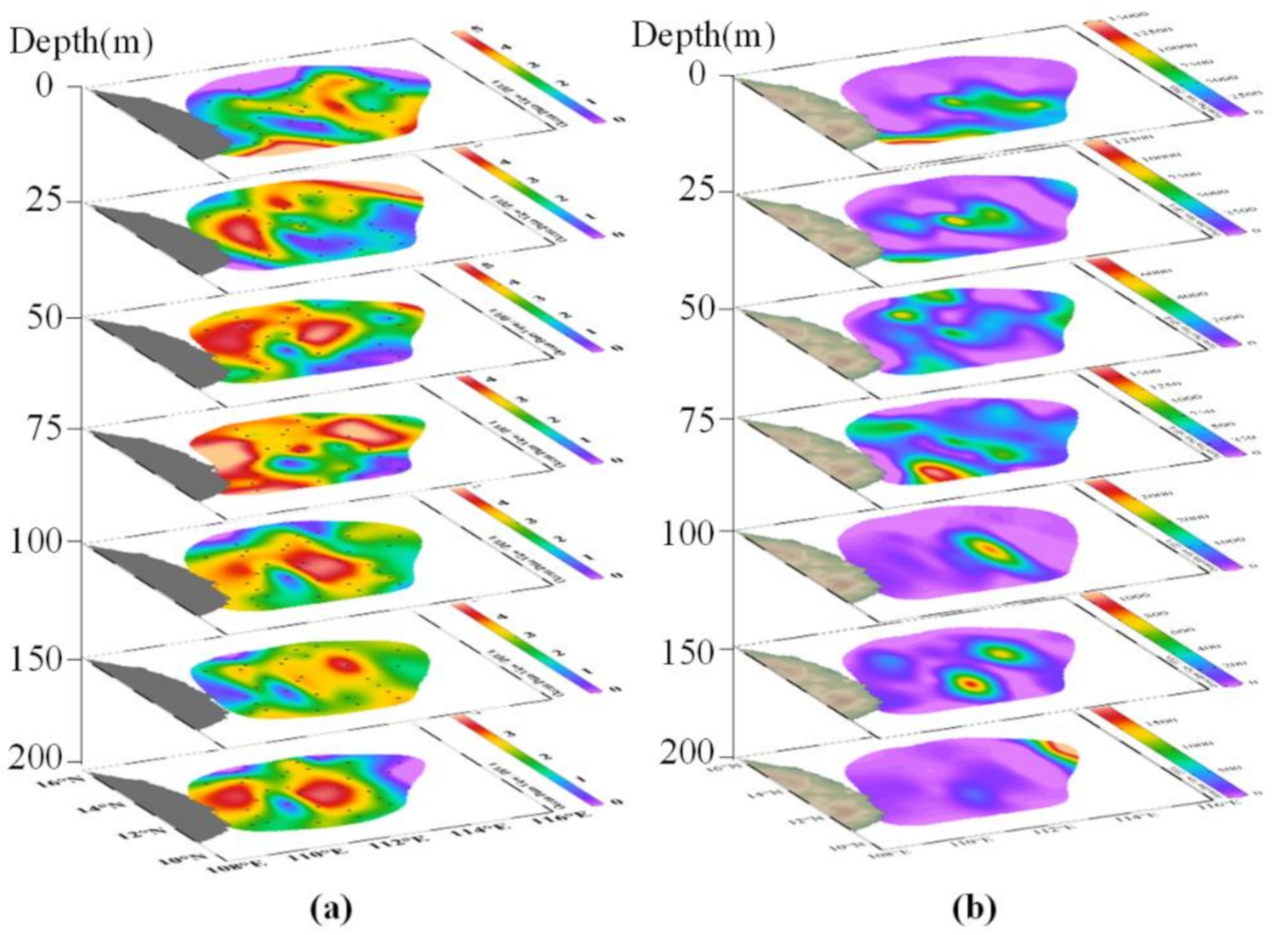
Figure A2.
Horizontal distributions of cyanobacteria (Cyano) and other phytoplankton (Phyto) abundances at the different water layers in summer.
Figure A2.
Horizontal distributions of cyanobacteria (Cyano) and other phytoplankton (Phyto) abundances at the different water layers in summer.

Figure A3.
The phytoplankton group difference among defined stages by Kruskal–Wallis test (**: p < 0.01, A: winter, B: summer, C: warm eddy, D: Eddy II, E: Eddy I, F: Eddy I relaxation, a: phytoplankton, b: diatom, c: dinoflagellate, and d: others).
Figure A3.
The phytoplankton group difference among defined stages by Kruskal–Wallis test (**: p < 0.01, A: winter, B: summer, C: warm eddy, D: Eddy II, E: Eddy I, F: Eddy I relaxation, a: phytoplankton, b: diatom, c: dinoflagellate, and d: others).

Figure A4.
Alpha diversity indices were analyzed between the two seasons (*: 0.01 < p < 0.05, ***: p < 0.001).
Figure A4.
Alpha diversity indices were analyzed between the two seasons (*: 0.01 < p < 0.05, ***: p < 0.001).

References
- Voss, M.; Bombar, D.; Loick, N.; Dippner, J.W. Riverine influence on nitrogen fixation in the upwelling region off Vietnam, South China Sea. Geophys. Res. Lett. 2006, 33, L07604. [Google Scholar] [CrossRef]
- Cai, W.-J.; Dai, M.; Wang, Y.; Zhai, W.; Huang, T.; Chen, S.; Zhang, F.; Chen, Z.; Wang, Z. The biogeochemistry of inorganic carbon and nutrients in the Pearl River estuary and the adjacent Northern South China Sea. Cont. Shelf Res. 2004, 24, 1301–1319. [Google Scholar] [CrossRef]
- Guo, M.; Chai, F.; Xiu, P.; Li, S.; Rao, S. Impacts of mesoscale eddies in the South China Sea on biogeochemical cycles. Ocean Dyn. 2015, 65, 1335–1352. [Google Scholar] [CrossRef]
- Yang, H.; Liu, Q.; Liu, Z.; Wang, D.; Liu, X. A general circulation model study of the dynamics of the upper ocean circulation of the South China Sea. J. Geophys. Res. 2002, 107. [Google Scholar] [CrossRef]
- Cheng, Z.D. Fluxes of seawater and some dissolved chemicals in the Bashi Strait. Chin. J. Oceanol. Limnol. 1995, 13, 240–246. [Google Scholar]
- Dippner, J.W.; Nguyen, K.V.; Hein, H.; Ohde, T.; Loick, N. Monsoon-induced upwelling off the Vietnamese coast. Ocean Dyn. 2007, 57, 46–62. [Google Scholar] [CrossRef]
- Gong, G.-C.; Liu, K.K.; Liu, C.-T.; Pai, S.-C. The chemical hydrography of the South China Sea west of Luzon and a comparison with the west Philippine Sea. Terr. Atmos. Ocean. Sci. 1992, 3, 587–602. [Google Scholar] [CrossRef]
- Chen, Y.-L.L.; Chen, H.-Y.; Karl, D.M.; Takahashi, M. Nitrogen modulates phytoplankton growth in spring in the South China Sea. Cont. Shelf Res. 2004, 24, 527–541. [Google Scholar] [CrossRef]
- Chen, Y.-L.L.; Chen, H.-Y.; Lin, I.-I.; Lee, M.-A.; Chang, J. Effects of cold eddy on phytoplankton production and assemblages in Luzon strait bordering the South China Sea. J. Oceanogr. 2007, 63, 671–683. [Google Scholar] [CrossRef]
- Liu, K.-K.; Chao, S.-Y.; Shaw, P.-T.; Gong, G.-C.; Chen, C.-C.; Tang, T. Monsoon-forced chlorophyll distribution and primary production in the South China Sea: Observational and a numerical study. Deep Sea Res. Part I Oceanogr. Res. Pap. 2002, 49, 1387–1412. [Google Scholar] [CrossRef]
- Loick-Wilde, N.; Bombar, D.; Doan, H.N.; Nguyen, L.N.; Nguyen-Thi, A.M.; Voss, M.; Dippner, J.W. Microplankton biomass and diversity in the Vietnamese upwelling area during SW monsoon under normal conditions and after an ENSO event. Prog. Oceanogr. 2017, 153, 1–15. [Google Scholar] [CrossRef]
- Sun, J.; Liu, D.Y. Net-phytoplankton community of the Bohai Sea in the autumn of 2000. Acta Oceanol. Sin. 2005, 27, 124–132. [Google Scholar]
- Guo, S.; Feng, Y.; Wang, L.; Dai, M.; Liu, Z.; Bai, Y.; Jun, S. Seasonal variation in the phytoplankton community of a continental-shelf sea: The East China Sea. Mar. Ecol. Prog. Ser. 2014, 516, 103–126. [Google Scholar] [CrossRef] [Green Version]
- Xue, B.; Sun, J.; Li, T.T. Phytoplankton community structure of northern South China Sea in summer of 2014. Acta Oceanol. Sin. 2016, 38, 54–65. [Google Scholar]
- Gan, J.; Li, H.; Curchitser, E.N.; Haidvogel, D.B. Modeling South China Sea circulation: Response to seasonal forcing regimes. J. Geophys. Res. Ocean. 2006, 111. [Google Scholar] [CrossRef]
- Wang, G.; Chen, D.; Su, J. Generation and life cycle of the dipole in the South China Sea summer circulation. J. Geophys. Res. Ocean. 2006, 111. [Google Scholar] [CrossRef] [Green Version]
- Ning, X.; Chai, F.; Xue, H.; Cai, Y.; Liu, C.; Shi, J. Physical-biological oceanographic coupling influencing phytoplankton and primary production in the South China Sea. J. Geophys. Res. 2004, 109. [Google Scholar] [CrossRef] [Green Version]
- Field, C.B.; Behrenfeld, M.J.; Randerson, J.T.; Falkowski, P. Primary production of the biosphere: Integrating terrestrial and oceanic components. Science 1998, 281, 237–240. [Google Scholar] [CrossRef] [PubMed] [Green Version]
- Mahadevan, A. The Impact of submesoscale physics on primary productivity of plankton. Ann. Rev. Mar. Sci. 2016, 8, 161–184. [Google Scholar] [CrossRef] [Green Version]
- Zhong, C.; Xiao, W.P.; Huang, B.Q. The response of phytoplankton to mesoscale eddies in western South China Sea. Adv. Mar. Sci. 2013, 31, 213–220. [Google Scholar]
- Tang, D.; Kawamura, H.; Van Dien, T.; Lee, M. Offshore phytoplankton biomass increase and its oceanographic causes in the South China Sea. Mar. Ecol. Prog. Ser. 2004, 268, 31–41. [Google Scholar] [CrossRef]
- Tang, D.L.; Kawamura, H.; Doan-Nhu, H.; Takahashi, W. Remote sensing oceanography of a harmful algal bloom off the coast of southeastern Vietnam. J. Geophys. Res. 2004, 109. [Google Scholar] [CrossRef]
- Wang, J.J.; Tang, D.L. Phytoplankton patchiness during spring intermonsoon in western coast of South China Sea. Deep Sea Res. II Top. Stud. Oceanogr. 2014, 101, 120–128. [Google Scholar] [CrossRef]
- Liang, Y.; Yuan, D.; Li, Q.; Lin, Q. Flow injection analysis of nanomolar level orthophosphate in seawater with solid phase enrichment and colorimetric detection. Mar. Chem. 2007, 103, 122–130. [Google Scholar] [CrossRef]
- Wang, L.; Huang, B.; Chiang, K.-P.; Liu, X.; Chen, B.; Xie, Y.; Hu, J.Y.; Dai, M.H. Physical-biological coupling in the western South China Sea: The response of phytoplankton community to a mesoscale cyclonic eddy. PLoS ONE 2016, 11, e0153735. [Google Scholar] [CrossRef] [PubMed]
- Ke, Z.; Tan, Y.; Huang, L.; Zhang, J.; Lian, S. Relationship between phytoplankton composition and environmental factors in the surface waters of southern South China Sea in early summer of 2009. Acta Oceanol. Sin. 2012, 31, 109–119. [Google Scholar] [CrossRef] [Green Version]
- Liang, W.; Tang, D.; Luo, X. Phytoplankton size structure in the western South China Sea under the influence of a ‘jet-eddy system’. J. Mar. Syst. 2018, 187, 82–95. [Google Scholar] [CrossRef]
- Falkowski, P.G.; Barber, R.T.; Smetacek, V. Biogeochemical controls and feedbacks on ocean primary production. Science 1998, 281, 200–206. [Google Scholar] [CrossRef] [Green Version]
- Hu, J.; Gan, J.; Sun, Z.; Zhu, J.; Dai, M. Observed three-dimensional structure of a cold eddy in the southwestern South China Sea. J. Geophys. Res. 2011, 116. [Google Scholar] [CrossRef]
- Fang, W.D.; Fang, G.H.; Shi, P.; Huang, Q.Z.; Xie, Q. Seasonal structures of upper layer circulation in the southern South China Sea from in situ observations. J. Geophys. Res. 2002, 107, 1–12. [Google Scholar] [CrossRef]
- Shaw, P.T.; Chao, S.Y. Surface circulation in the South China Sea. Deep Sea Res. Part I Oceanogr. Res. Pap. 1994, 41, 1663–1683. [Google Scholar] [CrossRef]
- Yuan, Y.C.; Liu, Y.G.; Liao, G.H.; Lou, R.Y.; Su, J.L.; Wang, K.S. Calculation of circulation in the South China Sea during summer of 2000 by the modified inverse method. Acta Oceanol. Sin. 2005, 24, 14–30. [Google Scholar] [CrossRef] [Green Version]
- Lin, H.; Hu, J.; Liu, Z.; Belkin, I.M.; Sun, Z.; Zhu, J. A peculiar lens-shaped structure observed in the South China Sea. Sci. Rep. 2017, 7, 478. [Google Scholar] [CrossRef] [PubMed] [Green Version]
- Xu, Y.P. Nutrient Dynamics Associated with Mesoscale Eddies in the Western South China Sea. Master’s Dissertation, Xiamen University, Xiamen, China, 2009. [Google Scholar]
- Liu, Q.; Kaneko, A.; Su, J.L. Recent progress in studies of the South China Sea circulation. J. Oceanogr. 2008, 64, 753–762. [Google Scholar] [CrossRef]
- Sun, J.; Liu, D.; Qian, S. A quantative research and analysis method for marine phytoplankton: An introduction to utermöhl method and its modification. J. Oceanogr. Huanghai Bohai Seas 2002, 20, 105–112. [Google Scholar]
- Sun, J.; Liu, D.Y.; Feng, S.Z. Preliminary study on marine phytoplankton sampling and analysis strategy for ecosystem dynamic research in coastal waters. Oceanol. Limnol. Sin. 2003, 34, 224–232. [Google Scholar]
- Sun, J.; Liu, D.Y. The preliminary notion on nomenclature of common phytoplankton in China seas waters. Oceanol. Limnol. Sin. 2002, 33, 271–286. [Google Scholar]
- Dai, M.; Wang, L.; Guo, X.; Zhai, W.; Li, Q.; He, B.; Kao, S.-J. Nitrification and inorganic nitrogen distribution in a large perturbed river/estuarine system: The Pearl River estuary, China. Biogeosciences 2008, 5, 1227–1244. [Google Scholar] [CrossRef] [Green Version]
- Pai, S.-C.; Yang, C.-C.; Riley, J.P. Effects of acidity and molybdate concentration on the kinetics of the formation of the phosphoantimonylmolybdenum blue complex. Anal. Chim. Acta 1990, 229, 115–120. [Google Scholar]
- Ma, J.; Yuan, D.; Liang, Y.; Dai, M.H. A modified analytical method for the shipboard determination of nanomolar concentrations of orthophosphate in seawater. J. Oceanogr. 2008, 64, 443–449. [Google Scholar] [CrossRef]
- Schlitzer, R. Ocean Data View. 2018. Available online: https://odv.awi.de (accessed on 2 March 2018).
- Sun, J.; Liu, D.Y. The application of diversity indices in marine phytoplankton studies. Acta Oceanol. Sin. 2004, 26, 62–75. [Google Scholar]
- RCRTeam. R: A Language and Environment for Statistical Computing, Version 3.6.1. Vienna, Austria. 2019. Available online: http://www.R-project.org/ (accessed on 5 July 2019).
- Zhu, G.H.; Ning, X.R.; Cai, Y.M.; Liu, Z.L.; Liu, C.G. Studies on species composition and abundance distribution of phytoplankton in the South China Sea. Haiyang Xuebao 2003, 25, 8–23. (In Chinese) [Google Scholar]
- Ke, Z.X.; Huang, L.M.; Tan, Y.H.; Yin, J.Q. Species composition and abundance of phytoplankton in the northern South China Sea in summer 2007. J. Trop. Oceanogr. 2011, 30, 131–143. [Google Scholar]
- Li, X.; Sun, J.; Tian, W.; Wang, M. Phytoplankton community in the northern area of South China Sea in summer of 2009. Mar. Sci. 2012, 36, 33–39. (In Chinese) [Google Scholar]
- Ma, W.; Sun, J. Characteristics of phytoplankton community in the northern South China Sea in summer and winter. Acta Ecol. Sin. 2014, 34, 621–632. (In Chinese) [Google Scholar]
- Wang, X.; Wei, Y.; Wu, C.; Guo, C.; Sun, J. The profound influence of Kuroshio intrusion on microphytoplankton community in the northeastern South China Sea. Acta Oceanol. Sin. 2020, 39, 79–87. [Google Scholar] [CrossRef]
- Zhong, Q.; Xue, B.; Noman, M.A.; Wei, Y.; Sun, J. Effect of river plume on phytoplankton community structure in Zhujiang River estuary. J. Oceanol. Limnol. 2020, 39, 550–565. [Google Scholar] [CrossRef]
- Chen, G.; Xiu, P.; Chai, F. Physical and biological controls on the summer chlorophyll bloom to the east of Vietnam. J. Oceanogr. 2014, 70, 323–328. [Google Scholar] [CrossRef]
- Martin, A.P.; Pondaven, P. On estimates for the vertical nitrate flux due to eddy pumping. J. Geophys. Res. Ocean. 2003, 108, 3359. [Google Scholar] [CrossRef]
- McGillicuddy, D.J.; Anderson, L.A.; Bates, N.R.; Bibby, T.; Buesseler, K.O.; Carlson, C.; Carlson, C.; Davis, C.S.; Ewart, C.; Falkowski, P.G.; et al. Eddy/wind interactions stimulate extraordinary mid-ocean plankton blooms. Science 2007, 316, 1021–1026. [Google Scholar] [CrossRef] [PubMed]
- Kumar, S.P.; Nuncio, M.; Ramaiah, N.; Sardesai, S.; Narvekar, J.; Fernandes, V.; Paul, J.T. Eddy-mediated biological productivity in the Bay of Bengal during fall and spring intermonsoons. Deep Sea Res. Part I Oceanogr. Res. Pap. 2007, 54, 1619–1640. [Google Scholar] [CrossRef] [Green Version]
- Edwards, K.F.; Litchman, E.; Klausmeier, C.A. Functional traits explain phytoplankton community structure and seasonal dynamics in a marine ecosystem. Ecol. Lett. 2013, 16, 56–63. [Google Scholar] [CrossRef]
- Boyd, P.W.; Hutchins, D.A. Understanding the responses of ocean biota to a complex matrix of cumulative anthropogenic change. Mar. Ecol. Prog. Ser. 2012, 470, 125–135. [Google Scholar] [CrossRef] [Green Version]
- Edwards, M.; Richardson, A.J. Impact of climate change on marine pelagic phenology and trophic mismatch. Nature 2004, 430, 881–884. [Google Scholar] [CrossRef]
- Zehr, J.P.; Capone, D.G. Changing perspectives in marine nitrogen fixation. Science 2020, 368. [Google Scholar] [CrossRef]
- Xiao, W.; Wang, L.; Laws, E.; Xie, Y.; Chen, J.; Liu, X.; Chen, B.; Huang, B. Realized niches explain spatial gradients in seasonal abundance of phytoplankton groups in the South China Sea. Prog. Oceanogr. 2018. [Google Scholar] [CrossRef]
- Chen, C.-T.A.; Wang, S.-L.; Wang, B.-J.; Pai, S.-C. Nutrient budgets for the South China Sea basin. Mar. Chem. 2001, 75, 281–300. [Google Scholar] [CrossRef]
- Zhang, Y.; Zhao, Z.; Sun, J.; Jiao, N. Diversity and distribution of diazotrophic communities in the South China Sea deep basin with mesoscale cyclonic eddy perturbations. FEMS Microbiol. Ecol. 2011, 78, 417–427. [Google Scholar] [CrossRef] [Green Version]
- Moisander, P.H.; Beinart, R.A.; Voss, M.; Zehr, J.P. Diversity and abundance of diazotrophic microorganisms in the South China Sea during intermonsoon. ISME J. 2008, 2, 954–967. [Google Scholar] [CrossRef] [PubMed] [Green Version]
- Bonnet, S.; Berthelot, H.; Turk-Kubo, K.; Cornet-Barthaux, V.; Fawcett, S.; Berman-Frank, I.; Barani, A.; Grégori, G.; Dekaezemacker, J.; Benavides, M.; et al. Diazotroph derived nitrogen supports diatom growth in the south West Pacific: A quantitative study using nanosims. Limnol. Oceanogr. 2016, 61, 1549–1562. [Google Scholar] [CrossRef] [Green Version]
- Carpenter, E.J.; Montoya, J.P.; Burns, J.; Mulholland, M.; Subramaniam, A.; Capone, D.G. Extensive bloom of N2-fixing diatom/cyanobacterial association in the tropical Atlantic Ocean. Mar. Ecol. Prog. Ser. 1999, 185, 273–283. [Google Scholar] [CrossRef] [Green Version]
- Foster, R.A.; Zehr, J.P. Characterization of diatom-cyanobacteria symbioses on the basis of nifH, hetR, and 16S rRNA sequences. Environ. Microbiol. 2006, 8, 1913–1925. [Google Scholar] [CrossRef]
- Foster, R.A.; Subramaniam, A.; Mahaffey, C.; Carpenter, E.J.; Capone, D.G.; Zehr, J.P. Influence of the Amazon River plume on distributions of free-living and symbiotic cyanobacteria in the western tropical North Atlantic Ocean. Limnol. Oceanogr. 2007, 52, 517–532. [Google Scholar] [CrossRef] [Green Version]
- Foster, R.A.; Goebel, N.L.; Zehr, J.P. Isolation of Calothrix Rhizosoleniae (Cyanobacteria) strain SC01 from Chaetoceros (Bacillariophyta) spp. diatoms of the Subtropical North Pacific Ocean. J. Phycol. 2010, 46, 1028–1037. [Google Scholar] [CrossRef]
- Foster, R.A.; Kuypers, M.M.M.; Vagner, T.; Paerl, R.W.; Musat, N.; Zehr, J.P. Nitrogen fixation and transfer in open ocean diatom-cyanobacterial symbioses. ISME J. 2011, 5, 1484–1493. [Google Scholar] [CrossRef] [Green Version]
- Cheng, L.; Trenberth, K.E.; Fasullo, J.; Boyer, T.; Abraham, J.; Zhu, J. Improved estimates of ocean heat content from 1960 to 2015. Sci. Adv. 2017, 3, e1601545. [Google Scholar] [CrossRef] [Green Version]
- Bopp, L.; Monfray, P.; Aumont, O.; Dufresne, J.-L.; Le Treut, H.; Madec, G.; Terray, L.; Orr, J.C. Potential impact of climate change on marine export production. Glob. Biogeochem. Cycles 2001, 15, 81–99. [Google Scholar] [CrossRef] [Green Version]
- Reynolds, S.E.; Mather, R.L.; Wolff, G.A.; Williams, R.G.; Landolfi, A.; Sanders, R.; Woodward, E.M.S. How widespread and important is N2 fixation in the North Atlantic Ocean? Glob. Biogeochem. Cycles 2007, 21. [Google Scholar] [CrossRef] [Green Version]
- Huertas, I.E.; Rouco, M.; Lopez-Rodas, V.; Costas, E. Warming will affect phytoplankton differently: Evidence through a mechanistic approach. Proc. R. Soc. B Biol. Sci. 2011, 278, 3534–3543. [Google Scholar] [CrossRef] [Green Version]
- Thomas, M.K.; Kremer, C.T.; Klausmeier, C.A.; Litchman, E. A global pattern of thermal adaptation in marine phytoplankton. Science 2012, 338, 1085–1088. [Google Scholar] [CrossRef] [PubMed] [Green Version]
- Hobday, A.J.; Alexander, L.V.; Perkins, S.E.; Smale, D.A.; Straub, S.C.; Oliver, E.C.J.; Benthuysen, J.A.; Burrows, M.T.; Donat, M.G.; Feng, M.; et al. A hierarchical approach to defining marine heatwaves. Prog. Oceanogr. 2016, 141, 227–238. [Google Scholar] [CrossRef] [Green Version]
- Oliver, E.C.J.; Donat, M.G.; Burrows, M.T.; Moore, P.J.; Smale, D.A.; Alexander, L.V.; Benthuysen, J.A.; Feng, M.; Sen Gupta, A.; Hobday, A.J.; et al. Longer and more frequent marine heatwaves over the past century. Nat. Commun. 2018, 9, 1324. [Google Scholar] [CrossRef] [PubMed]
- Wernberg, T.; Bennett, S.; Babcock, R.C.; De Bettignies, T.; Cure, K.; Depczynski, M.; Dufois, F.; Fromont, J.; Fulton, C.J.; Hovey, R.K.; et al. Climate-driven regime shift of a temperate marine ecosystem. Science 2016, 353, 169–172. [Google Scholar] [CrossRef] [PubMed] [Green Version]
- Bond, N.A.; Cronin, M.F.; Freeland, H.; Mantua, N. Causes and impacts of the 2014 warm anomaly in the NE Pacific. Geophys. Res. Lett. 2015, 42, 3414–3420. [Google Scholar] [CrossRef]
- Irwin, A.J.; Finkel, Z.V.; Müller-Karger, F.E.; Ghinaglia, L.T. Phytoplankton adapt to changing ocean environments. Proc. Natl. Acad. Sci. USA 2015, 112, 5762–5766. [Google Scholar] [CrossRef] [Green Version]
- Liang, Y.; Koester, J.A.; Liefer, J.D.; Irwin, A.J.; Finkel, Z.V. Molecular mechanisms of temperature acclimation and adaptation in marine diatoms. ISME J. 2019, 13, 2415–2425. [Google Scholar] [CrossRef] [PubMed]
- Mao, Y.; Sun, J.; Guo, C.; Wei, Y.; Wang, X.; Yang, S.; Wu, C. Effects of typhoon Roke and Haitang on phytoplankton community structure in northeastern South China Sea. Ecosyst. Health Sustain. 2019, 5, 144–154. [Google Scholar] [CrossRef] [Green Version]
- Liu, H.; Wu, C.; Xu, W.; Wang, X.; Thangaraj, S.; Zhang, G.; Zhang, X.; Zhao, Y.; Sun, J. Surface phytoplankton assemblages and controlling factors in the strait of Malacca and Sunda Shelf. Front. Mar. Sci. 2019, 7, 33. [Google Scholar] [CrossRef]
- Moore, C.M.; Mills, M.M.; Arrigo, K.R.; Berman-Frank, I.; Bopp, L.; Boyd, P.W.; Galbraith, E.D.; Geider, R.J.; Guieu, C.; Jaccard, S.L.; et al. Processes and patterns of oceanic nutrient limitation. Nat. Geosci. 2013, 6, 701–710. [Google Scholar] [CrossRef] [Green Version]
Figure 1.
Map indicating the sampling stations along the southwestern region of the South China Sea (SCS) (Vietnamese upwelling region) (A). The arrows indicate the general surface current patterns in the SCS during the winter (black dotted arrows) and summer (black solid arrows) [35]. Map indicating the sampling locations during the winter (B) and summer seasons. The red dotted circle shows the eddy area, i.e., CE1: cold eddy 1, CE2: cold eddy 2, and WE: warm eddy [29,35]. The blue dotted lines show sampling sections defined as Section A, Section B, Section C, and Section D.

Figure 2.
Composition and abundance (cell L−1) of phytoplankton community in the surface water in the winter (A) and summer (B), and vertical distribution (station average) patterns of phytoplankton group relative abundance (%) in the winter (C) and summer (D).
Figure 2.
Composition and abundance (cell L−1) of phytoplankton community in the surface water in the winter (A) and summer (B), and vertical distribution (station average) patterns of phytoplankton group relative abundance (%) in the winter (C) and summer (D).

Figure 3.
Vertical distribution of phytoplankton abundance during the summer. (a) Phytoplankton (Phyto) excluding cyanobacteria; (b) cyanobacteria (Cyano). CE1: cold eddy 1, CE2: cold eddy 2, and WE: warm eddy.
Figure 3.
Vertical distribution of phytoplankton abundance during the summer. (a) Phytoplankton (Phyto) excluding cyanobacteria; (b) cyanobacteria (Cyano). CE1: cold eddy 1, CE2: cold eddy 2, and WE: warm eddy.

Figure 4.
The relative abundance (%) contribution of different groups to the phytoplankton community (a), and the vertical variation of phytoplankton abundance (cell L−1) at different eddy stages (b). (NE: winter, CE1: cold eddy 1, CE1-r: cold eddy 1 relaxation, CE2: cold eddy 2, and WE: warm eddy).

Figure 5.
Shannon–Wiener diversity index (H’) (a) and cell abundance (b) of the phytoplankton community at different layers in summer.
Figure 5.
Shannon–Wiener diversity index (H’) (a) and cell abundance (b) of the phytoplankton community at different layers in summer.

Figure 6.
The influence of the environmental factors on the phytoplankton community shown with Spearman’s correlation and CCA value, respectively. Notes: (A,B) represents Spearman’s correlation and CCA for the winter samples, and (C,D) represents Spearman’s correlation and CCA for the summer samples. Environmental parameters include temperature (T), salinity (S), depth (Dep), PO43− (P), N: NOx (P), SiO32− (Si), N/P ratio, and Si/N ratio. Phytoplankton are listed as the following groups: diatoms G1 to G3 represent Bacteriastrum, Chaetoceros, and Rhizosolenia, belonging to the class of Centricae, G4 to G6 represent Fragilariaceae, Naviculaceae, and Nitzschiaceae, belonging to the class of Pennatae, and G7 to G9 represent Dictyocha, Trichodesmium, and symbionts. Dia: diatom, Din: dinoflagellate, Cya: cyanobacteria, and Phy: phytoplankton.

Table 1.
List of the dominant phytoplankton species (with their occurrence frequency f and dominance index Y) observed during the winter and summer seasons in the southwestern South China Sea.
Table 1.
List of the dominant phytoplankton species (with their occurrence frequency f and dominance index Y) observed during the winter and summer seasons in the southwestern South China Sea.
| Winter | Summer | ||||
|---|---|---|---|---|---|
| Species | f | Y | Species | f | Y |
| Thalassionema nitzschioides | 0.23 | 0.0231 | Trichodesmium thiebautii | 0.29 | 0.1842 |
| Nitzschia spp. | 0.33 | 0.0136 | Thalassionema nitzschioides | 0.57 | 0.0171 |
| Trichodesmium thiebautii | 0.05 | 0.0120 | Trichodesmium erythraeum | 0.13 | 0.0071 |
| Thalassiosira rotula | 0.30 | 0.0102 | Chaetoceros dichaeta | 0.28 | 0.0066 |
| Navicula spp. | 0.28 | 0.0089 | Chaetoceros affinis | 0.40 | 0.0054 |
| Chaetoceros spp. | 0.23 | 0.0081 | Thalassionema frauenfeldii | 0.54 | 0.0052 |
| Bacteriastrum spp. | 0.13 | 0.0066 | Chaetoceros lorenzianus | 0.30 | 0.0043 |
| Dictyocha fibula | 0.25 | 0.0057 | Pseudo-nitzschia delicatissima | 0.35 | 0.0041 |
| Thalassiosira subtilis | 0.20 | 0.0049 | Pseudo-nitzschia pungens | 0.28 | 0.0030 |
| Chaetoceros affinis | 0.08 | 0.0019 | Leptocylindrus danicus | 0.30 | 0.0026 |
| Chaetoceros coarctatus | 0.05 | 0.0016 | Hemiaulus hauckii | 0.37 | 0.0025 |
| Chaetoceros lorenzianus | 0.03 | 0.0014 | Nitzschia spp. | 0.65 | 0.0025 |
| Corethron hystrix | 0.05 | 0.0013 | Navicula spp. | 0.68 | 0.0022 |
| Chaetoceros atlanticus | 0.10 | 0.0008 | Bacteriastrum comosum | 0.23 | 0.0020 |
| Chaetoceros laciniosus | 0.05 | 0.0007 | Bacteriastrum hyalinum | 0.20 | 0.0019 |
| Thalassiothrix frauenfeldii | 0.05 | 0.0006 | Chaetoceros messanense | 0.23 | 0.0015 |
| Rizizosoleniu Rhizosolenia hebetata-Richelia | 0.08 | 0.0005 | Chaetoceros curvisetus | 0.14 | 0.0013 |
| Rhizosolenia hebetata | 0.03 | 0.0005 | Chaetoceros tortissimus | 0.16 | 0.0013 |
| Octactis octonaria | 0.08 | 0.0004 | Bacteriastrum elongatum | 0.21 | 0.0012 |
| Leptocylindrus mediterraneus | 0.03 | 0.0004 | Dactyliosolen blavyanus | 0.36 | 0.0010 |
Table 2.
Comparison of historical data of phytoplankton with average cell abundance in the South China Sea.
Table 2.
Comparison of historical data of phytoplankton with average cell abundance in the South China Sea.
| Sampling Date | Region | Water Depth (m) | Species Number | Abundance (103 cell L−1) | Reference |
|---|---|---|---|---|---|
| 1998–06–07 | 6–23° N,108–120° E | 0–150 m | 88 | 0.84 | [17] |
| 1998.06 | 5–25° N,105–120° E | Surface | 63 | 0.83 | [45] |
| 1998.08 | 18–22° N, 105–117° E | Surface | 58 | 181.00 | [45] |
| 1998.11–12 | 18–22° N, 105–117° E | 0–150 m | 85 | 8.46 | [17] |
| 2006.12 | 10–15° N, 110–112.5° E | 0–200 m | 117 | 2.74 | This study |
| 2007.08–09 | 10–15° N, 110–112.5° E | 0–200 m | 314 | 1.05 | This study |
| 2007.08 | 18–22° N, 110–120° E | 0–200 m | 216 | 11.22 | [46] |
| 2009.08 | 18–22° N, 110–117° E | 0–200 m | 109 | 8.20 | [47] |
| 2009.07–08 | 18–23.5° N, 109–120° E | 0–200 m | 150 | 26.49 | [48] |
| 2014.08 | 18–22° N, 114–116° E | 0–200 m | 229 | 16.32 | [14] |
| 2014.08 | 18–22° N, 114–116° E | Surface | 98 | 0.23 | [14] |
| 2015.07–08 | 21–23.5° N, 111–117° E | 0–200 m | 212 | 45.61 | [49] |
| 2017.07–08 | 14–23° N, 114–124° E | 0–200 m | 287 | 2.14 | [50] |
Publisher’s Note: MDPI stays neutral with regard to jurisdictional claims in published maps and institutional affiliations. |
© 2021 by the authors. Licensee MDPI, Basel, Switzerland. This article is an open access article distributed under the terms and conditions of the Creative Commons Attribution (CC BY) license (https://creativecommons.org/licenses/by/4.0/).
Share and Cite
MDPI and ACS Style
Ding, C.; Sun, J.; Narale, D.D.; Liu, H. Phytoplankton Community in the Western South China Sea in Winter and Summer. Water 2021, 13, 1209. https://doi.org/10.3390/w13091209
AMA Style
Ding C, Sun J, Narale DD, Liu H. Phytoplankton Community in the Western South China Sea in Winter and Summer. Water. 2021; 13(9):1209. https://doi.org/10.3390/w13091209
Chicago/Turabian StyleDing, Changling, Jun Sun, Dhiraj Dhondiram Narale, and Haijiao Liu. 2021. "Phytoplankton Community in the Western South China Sea in Winter and Summer" Water 13, no. 9: 1209. https://doi.org/10.3390/w13091209
Note that from the first issue of 2016, this journal uses article numbers instead of page numbers. See further details here.